DOMAIN DECOMPOSITION AND MULTISCALE MORTAR MIXED FINITE ELEMENT METHODS FOR LINEAR ELASTICITY WITH WEAK STRESS SYMMETRY

Abstract

Two non-overlapping domain decomposition methods are presented for the mixed finite element formulation of linear elasticity with weakly enforced stress symmetry. The methods utilize either displacement or normal stress Lagrange multiplier to impose interface continuity of normal stress or displacement, respectively. By eliminating the interior subdomain variables, the global problem is reduced to an interface problem, which is then solved by an iterative procedure. The condition number of the resulting algebraic interface problem is analyzed for both methods. A multiscale mortar mixed finite element method for the problem of interest on non-matching multiblock grids is also studied. It uses a coarse scale mortar finite element space on the non-matching interfaces to approximate the trace of the displacement and impose weakly the continuity of normal stress. A priori error analysis is performed. It is shown that, with appropriate choice of the mortar space, optimal convergence on the fine scale is obtained for the stress, displacement, and rotation, as well as some superconvergence for the displacement. Computational results are presented in confirmation of the theory of all proposed methods.

65N30, 65N55, 65N12, 74G15

1 Introduction

Mixed finite element (MFE) methods for elasticity are important computational tools due to their local momentum conservation, robust approximation of the stress, and non-locking behavior for almost incompressible materials. In this paper, we focus on MFE methods with weakly imposed stress symmetry [1, 8, 42, 9, 12, 15, 26, 7, 11], since they allow for spaces with fewer degrees of freedom, as well as reduction to efficient finite volume schemes for the displacement [2, 3]. We note that the developments in this paper also apply to MFE methods for elasticity with strong stress symmetry.

In many physical applications, obtaining the desired resolution may result in a very large algebraic system. Therefore a critical component for the applicability of MFE methods for elasticity is the development of efficient techniques for the solution of these algebraic systems. Domain decomposition methods [43, 39] provide one such approach. They adopt the ”divide and conquer” strategy and split the computational domain into multiple non-overlapping subdomains. Then, solving the local problems of lower complexity with an appropriate choice of interface conditions leads to recovering the global solution. This approach naturally leads to designing parallel algorithms, and also allows for the reuse of existing codes for solving the local subdomain problems. Non-overlapping domain decomposition methods for non-mixed displacement-based elasticity formulations have been studied extensively [32, 30, 31, 20, 23, 28], see also [25, 36] for displacement-pressure mixed formulations. To the best of our knowledge, non-overlapping domain decomposition methods for stress-displacement mixed elasticity formulations have not been studied.

In this paper, we develop two non-overlapping domain decomposition methods for the mixed finite element discretization of linear elasticity with weakly enforced stress symmetry. The first method uses a displacement Lagrange multiplier to impose interface continuity of the normal stress. The second method uses a normal stress Lagrange multiplier to impose interface continuity of the displacement. These methods can be thought of as elasticity analogs of the methods introduced in [24] for scalar second order elliptic problems, see also [16]. In both methods, the global system is reduced to an interface problem by eliminating the interior subdomain variables. We show that the interface operator is symmetric and positive definite, so the interface problem can be solved by the conjugate gradient method. Each iteration requires solving Dirichlet or Neumann subdomain problems. The condition number of the resulting algebraic interface problem is analyzed for both methods, showing that it is $O(h^{-1})$. We note that in the second method the Neumann subdomain problems can be singular. We deal with floating subdomains by following the approach from the FETI methods [19, 43], solving a coarse space problem to ensure that the subdomain problems are solvable.

We also develop a multiscale mortar mixed finite element method for the domain decomposition formulation of linear elasticity with non-matching grids. We note that domains with complex geometries can be represented by unions of subdomains with simpler shapes that are meshed independently, resulting in non-matching grids across the interfaces. The continuity conditions are imposed using mortar finite elements, see e.g. [4, 20, 31, 30, 23, 37, 28]. Here we focus on the first formulation, using a mortar finite element space on the non-matching interfaces to approximate the trace of the displacement and impose weakly the continuity of normal stress. We allow for the mortar space to be on a coarse scale $H$, resulting in a multiscale approximation, see e.g. [38, 5, 22]. A priori error analysis is performed. It is shown that, with appropriate choice of the mortar space, optimal convergence on the fine scale is obtained for the stress, displacement, and rotation, as well as some superconvergence for the displacement.

The rest of the paper is organized as follows. The problem of interest, its MFE approximation, and the two domain decomposition methods are formulated in Section 2. The analysis of the resulting interface problems is presented in Section 3. The multiscale mortar MFE element method is developed and analyzed in Section 4. A multiscale stress basis implementation for the interface problem is also given in this section. The paper concludes with computational results in Section 5, which confirm the theoretical results on the condition number of the domain decomposition methods and the convergence of the solution of the multiscale mortar MFE element method.

2 Formulation of the methods

2.1 Model problem

Let $\Omega\subset\mathbb{R}^{d}$, $d=2,3$ be a simply connected bounded polygonal domain occupied by a linearly elastic body. Let $\mathbb{M}$, $\mathbb{S}$, and $\mathbb{N}$ be the spaces of $d\times d$ matrices, symmetric matrices, and skew-symmetric matrices over the field $\mathbb{R}$, respectively. The material properties are described at each point $x\in\Omega$ by a compliance tensor $A=A(x)$, which is a self-adjoint, bounded, and uniformly positive definite linear operator acting from $\mathbb{S}$ to $\mathbb{S}$. We assume that $A$ can be extended to an operator from $\mathbb{M}$ to $\mathbb{M}$ with the same properties. In particular, in the case of homogeneous and isotropic body,

(2.1) $$A\sigma=\frac{1}{2\mu}\left(\sigma-\frac{\lambda}{2\mu+d\lambda}\operatorname{tr}(\sigma)I\right),$$

where $I$ is the $d\times d$ identity matrix and $\mu>0,\lambda\geq 0$ are the Lamé coefficients.

Throughout the paper the divergence operator is the usual divergence for vector fields, which produces a vector field when applied to a matrix field by taking the divergence of each row. We will also use the curl operator which is the usual curl when applied to vector fields in three dimensions, and defined as $\operatorname{curl}{\phi}=(\partial_{2}\phi,-\partial_{1}\phi)^{T}$ for a scalar function $\phi$ in two dimensions. For a vector field in two dimensions or a matrix field in three dimensions, the curl operator produces a matrix field in two or three dimensions, respectively, by acting row-wise.

Given a vector field $f$ on $\Omega$ representing body forces, the equations of static elasticity in Hellinger-Reissner form determine the stress $\sigma$ and the displacement $u$ satisfying the following constitutive and equilibrium equations respectively, together with appropriate boundary conditions:

(2.2) $$A\sigma=\epsilon(u),\quad\operatorname{div}\sigma=f\,\,\text{ in }\Omega,$$

(2.3) $$u=g_{D}\,\,\text{ on }\Gamma_{D},\quad\sigma\,n=0\,\,\text{ on }\Gamma_{N},$$

where $\epsilon(u)=\frac{1}{2}(\nabla u+(\nabla u)^{T})$ and $n$ is the outward unit normal vector field on $\partial\Omega=\Gamma_{D}\cup\Gamma_{N}$. For simplicity we assume that $\operatorname{meas\,}(\Gamma_{D})>0$, in which case the problem (2.2)–(2.3) has a unique solution.

We will make use of the following standard notations. For a set $G\subset\mathbb{R}^{d}$, the $L^{2}(G)$ inner product and norm are denoted by $(\cdot,\cdot)_{G}$ and $\|\cdot\|_{G}$ respectively, for scalar, vector and tensor valued functions. For a section of a subdomain boundary $S$ we write $\langle\cdot,\cdot\rangle_{S}$ and $\|\cdot\|_{S}$ for the $L^{2}(S)$ inner product (or duality pairing) and norm, respectively. We omit subscript $G$ if $G=\Omega$ and $S$ if $S=\Gamma$. We also denote by $C$ a generic positive constant independent of the discretization parameters. We note that, using (2.1), we have

$$\left(A\sigma,\tau\right)=\frac{1}{2\mu}\left(\sigma,\tau\right)-\frac{\lambda}{2\mu(2\lambda+d\mu)}\left(\operatorname{tr\,}(\sigma),\operatorname{tr\,}(\tau)\right),$$

implying

(2.4) $$\frac{1}{2\mu+d\lambda}\|\sigma\|^{2}\leq\left(A\sigma,\sigma\right)\leq\frac{1}{2\mu}\|\sigma\|^{2}.$$

We consider the mixed variational formulation for (2.2)–(2.3) with weakly imposed stress symmetry. Introducing a rotation Lagrange multiplier $\gamma\in\mathbb{N}$ to penalize the asymmetry of the stress tensor, we obtain: find $(\sigma,u,\gamma)\in\mathbb{X}\times V\times\mathbb{W}$ such that

(2.5) $$\left(A\sigma,\tau\right)+\left(u,\operatorname{div}{\tau}\right)+\left(\gamma,\tau\right)=\left\langle g_{D},\tau\,n\right\rangle_{\Gamma_{D}}, \forall\tau \in\mathbb{X},$$

(2.6) $$\left(\operatorname{div}\sigma,v\right)=\left(f,v\right), \forall v \in V,$$

(2.7) $$\left(\sigma,\xi\right)=0, \forall\xi \in\mathbb{W},$$

where

$$\mathbb{X}=\big{\{}\tau\in H(\operatorname{div};\Omega,\mathbb{M}):\tau\,n=0\text{ on }\Gamma_{N}\big{\}},\quad V=L^{2}(\Omega,\mathbb{R}^{d}),\quad\mathbb{W}=L^{2}(\Omega,\mathbb{N}),$$

with norms

$$\|\tau\|_{\mathbb{X}}=\left(\|\tau\|^{2}+\|\operatorname{div}\tau\|^{2}\right)^{1/2},\quad\|v\|_{V}=\|v\|,\quad\|\xi\|_{\mathbb{W}}=\|\xi\|.$$

It is known [9] that (2.5)–(2.7) has a unique solution.

2.2 MFE approximation

In the first part of the paper we consider a global conforming shape regular and quasi-uniform finite element partition $\mathcal{T}_{h}$ of $\Omega$. We assume that $\mathcal{T}_{h}$ consists of simplices or rectangular elements, but note that the proposed methods can be extended to other types of elements for which stable elasticity MFE spaces have been developed, e.g., the quadrilateral elements in [7]. Let

$$\mathbb{X}_{h}\times V_{h}\times\mathbb{W}_{h}\subset\mathbb{X}\times V\times\mathbb{W}$$

be any stable triple of spaces for linear elasticity with weakly imposed stress symmetry, such as the Amara-Thomas [1], PEERS [8], Stenberg [42], Arnold-Falk-Winther [9, 7, 11], or Cockburn-Gopalakrishnan-Guzman [15, 26] families of elements. For all spaces $\operatorname{div}\mathbb{X}_{h}=V_{h}$ and there exists a projection operator $\Pi:H^{1}(\Omega,\mathbb{M})\to\mathbb{X}_{h}$, such that for any $\tau\in H^{1}(\Omega,\mathbb{M})$,

(2.8) $$\left(\operatorname{div}{(\Pi\,\tau-\tau)},v\right)_{\Omega}=0,\quad\forall\,v\in V_{h},$$

(2.9) $$\left\langle(\Pi\,\tau-\tau)\,n,\chi\,n\right\rangle_{\partial\Omega}=0,\quad\forall\,\chi\in\mathbb{X}_{h}.$$

The MFE approximation of (2.5)–(2.7) is: find $(\sigma_{h},u_{h},\gamma_{h})\in\mathbb{X}_{h}\times V_{h}\times\mathbb{W}_{h}$ such that

(2.10) $$\left(A\sigma_{h},\tau\right)+\left(u_{h},\operatorname{div}{\tau}\right)+\left(\gamma_{h},\tau\right)=\left\langle g_{D},\tau\,n\right\rangle_{\Gamma_{D}}, \forall\tau \in\mathbb{X}_{h},$$

(2.11) $$\left(\operatorname{div}\sigma_{h},v\right)=\left(f,v\right), \forall v \in V_{h},$$

(2.12) $$\left(\sigma_{h},\xi\right)=0, \forall\xi \in\mathbb{W}.$$

The well-posedness of (2.10)–(2.12) has been shown in the above-mentioned references. It was also shown in [9, 15, 26] that the following error estimate holds:

(2.13) $$\|\sigma-\sigma_{h}\|+\|\mathcal{P}_{h}u-u_{h}\|+\|\gamma-\gamma_{h}\|\leq C(\|\sigma-\Pi\sigma\|+\|\gamma-\mathcal{R}_{h}\gamma\|),$$

where $\mathcal{P}_{h}$ is the $L^{2}(\Omega)$-projection onto $V_{h}$ and $\mathcal{R}_{h}$ is the $L^{2}(\Omega)$-projection onto $\mathbb{W}_{h}$. Later we will also use the restrictions of the global projections on a subdomain $\Omega_{i}$, denoted as $\Pi_{i}$, $\mathcal{P}_{h,i}$, and $\mathcal{R}_{h,i}$.

2.3 Domain decomposition formulations

Let $\Omega=\cup_{i=1}^{n}\Omega_{i}$ be a union of nonoverlapping shape regular polygonal subdomains. Let $\Gamma_{i,j}=\partial\Omega_{i}\cap\partial\Omega_{j},\,\Gamma=\cup_{i,j=1}^{n}\Gamma_{i,j},$ and $\Gamma_{i}=\partial\Omega_{i}\cap\Gamma=\partial\Omega_{i}\setminus\partial\Omega$ denote the interior subdomain interfaces. Denote the restrictions of $\mathbb{X}_{h}$, $V_{h}$, and $\mathbb{W}_{h}$ to $\Omega_{i}$ by $\mathbb{X}_{h,i}$, $V_{h,i}$, and $\mathbb{W}_{h,i}$, respectively. Let $\mathcal{T}_{h,i,j}$ be a finite element partition of $\Gamma_{i,j}$ obtained from the trace of $\mathcal{T}_{h}$ and let $\Lambda_{h,i,j}=\mathbb{X}_{h}\,n$ be the Lagrange multiplier space on $\mathcal{T}_{h,i,j}$. Let $\Lambda_{h}=\bigoplus_{1\leq i,j\leq n}\Lambda_{h,i,j}$. We now present two domain decomposition formulations. The first one uses a displacement Lagrange multiplier to impose weakly continuity of normal stress.

Method 1: For $1\leq i\leq n$, find $(\sigma_{h,i},u_{h,i},\gamma_{h,i},\lambda_{h})\in\mathbb{X}_{h,i}\times V_{h,i}\times\mathbb{W}_{h,i}\times\Lambda_{h}$ such that

$$\left(A\sigma_{h,i},\tau\right)_{\Omega_{i}}+\left(u_{h,i},\operatorname{div}{\tau}\right)_{\Omega_{i}}+\left(\gamma_{h,i},\tau\right)_{\Omega_{i}}$$

(2.14) $$\qquad\qquad\qquad=\left\langle\lambda_{h},\tau\,n_{i}\right\rangle_{\Gamma_{i}}+\left\langle g_{D},\tau\,n_{i}\right\rangle_{\partial\Omega_{i}\cap\Gamma_{D}}, \forall\tau\in\mathbb{X}_{h,i},$$

(2.15) $$\left(\operatorname{div}\sigma_{h,i},v\right)_{\Omega_{i}}=\left(f,v\right)_{\Omega_{i}}, \forall v\in V_{h,i},$$

(2.16) $$\left(\sigma_{h,i},\xi\right)_{\Omega_{i}}=0, \forall\xi\in\mathbb{W}_{h,i},$$

(2.17) $$\sum_{i=1}^{n}\left\langle\sigma_{h,i}\,n_{i},\mu\right\rangle_{\Gamma_{i}}=0, \forall\mu\in\Lambda_{h},$$

where $n_{i}$ is the outward unit normal vector field on $\partial\Omega_{i}$. We note that the subdomain problems in the above method are of Dirichlet type.

The second method uses a normal stress Lagrange multiplier to impose weakly continuity of displacement. Let $\mathbb{X}_{h,i}^{0}=\{\tau\in\mathbb{X}_{h,i}:\tau\,n=0\mbox{ on }\Gamma\}$ and let $\mathbb{X}_{h}^{\Gamma}$ be the complementary subspace:

$$\mathbb{X}_{h}=\bigoplus\mathbb{X}_{h,1}^{0}\cdots\bigoplus\mathbb{X}_{h,n}^{0}\bigoplus\mathbb{X}_{h}^{\Gamma}.$$

Method 2: For $1\leq i\leq n$, find $(\sigma_{h,i},u_{h,i},\gamma_{h,i})\in\mathbb{X}_{h,i}\times V_{h,i}\times\mathbb{W}_{h,i}$ such that

(2.18) $$\left(A\sigma_{h,i},\tau\right)_{\Omega_{i}}+\left(u_{h,i},\operatorname{div}{\tau}\right)_{\Omega_{i}}+\left(\gamma_{h,i},\tau\right)_{\Omega_{i}}=\left\langle g_{D},\tau\,n_{i}\right\rangle_{\partial\Omega_{i}\cap\Gamma_{D}}, \forall\tau\in\mathbb{X}_{h,i}^{0},$$

(2.19) $$\left(\operatorname{div}\sigma_{h,i},v\right)_{\Omega_{i}}=\left(f,v\right)_{\Omega_{i}}, \forall v\in V_{h,i},$$

(2.20) $$\left(\sigma_{h,i},\xi\right)_{\Omega_{i}}=0, \forall\xi\in\mathbb{W}_{h,i},$$

(2.21) $$\sum_{i=1}^{n}\sigma_{h,i}\,n_{i}=0\quad\mbox{on }\Gamma,$$

(2.22) $$\sum_{i=1}^{n}\left[\left(A\sigma_{h,i},\tau\right)_{\Omega_{i}}+\left(u_{h,i},\operatorname{div}{\tau}\right)_{\Omega_{i}}+\left(\gamma_{h,i},\tau\right)_{\Omega_{i}}\right]=0, \forall\tau\in\mathbb{X}_{h}^{\Gamma}.$$

We note that (2.22) imposes weakly continuity of displacement on the interface, since taking $\tau\in\mathbb{X}_{h}^{\Gamma}$ in (2.18) and summing gives

$$0=\sum_{i=1}^{n}\left[\left(A\sigma_{h,i},\tau\right)_{\Omega_{i}}+\left(u_{h,i},\operatorname{div}{\tau}\right)_{\Omega_{i}}+\left(\gamma_{h,i},\tau\right)_{\Omega_{i}}\right]=\sum_{i=1}^{n}\left\langle u_{h,i},\tau\,n_{i}\right\rangle_{\Gamma}\quad\forall\tau\in\mathbb{X}_{h}^{\Gamma}.$$

It is easy to see that both (2.14)–(2.17) and (2.18)–(2.22) are equivalent to the global formulation (2.10)–(2.12) with $(\sigma_{h},u_{h},\gamma_{h})|_{\Omega_{i}}=(\sigma_{h,i},u_{h,i},\gamma_{h,i})$. In Method 1, $\lambda_{h}$ approximates $u|_{\Gamma}$.

3 Reduction to an interface problem and condition number analysis

3.1 Method 1

To reduce (2.14)–(2.17) to an interface problem for $\lambda_{h}$, we decompose the solution as

(3.1) $$\sigma_{h,i}=\sigma^{*}_{h,i}(\lambda_{h})+\bar{\sigma}_{h,i}, u_{h,i}=u^{*}_{h,i}(\lambda_{h})+\bar{u}_{h,i}, \gamma_{h,i}=\gamma^{*}_{h,i}(\lambda_{h})+\bar{\gamma}_{h,i},$$

where, for $\lambda_{h}\in\Lambda_{h}$, $\left(\sigma^{*}_{i}(\lambda_{h}),u_{i}^{*}(\lambda_{h}),\gamma^{*}_{i}(\lambda_{h})\right)\in\mathbb{X}_{h,i}\times V_{h,i}\times W_{h,i},\,1\leq i\leq n,$ solve

$$\left(A\sigma_{h,i}^{*}(\lambda_{h}),\tau\right)_{\Omega_{i}}+\left(u_{h,i}^{*}(\lambda_{h}),\operatorname{div}{\tau}\right)_{\Omega_{i}}+\left(\gamma_{h,i}^{*}(\lambda_{h}),\tau\right)_{\Omega_{i}}$$

(3.2) $$\qquad\qquad\qquad\qquad=\left\langle\lambda_{h},\tau\,n_{i}\right\rangle_{\Gamma_{i}}, \forall\tau \in\mathbb{X}_{h,i},$$

(3.3) $$\left(\operatorname{div}\sigma_{h,i}^{*}(\lambda_{h}),v\right)_{\Omega_{i}}=0, \forall v \in V_{h,i},$$

(3.4) $$\left(\sigma_{h,i}^{*}(\lambda_{h}),\xi\right)_{\Omega_{i}}=0, \forall\xi \in\mathbb{W}_{h,i},$$

and $(\bar{\sigma}_{h,i},\bar{u}_{h,i},\bar{\gamma}_{h,i})\in\mathbb{X}_{h,i}\times V_{h,i}\times\mathbb{W}_{h,i}$ solve

(3.5) $$\left(A\bar{\sigma}_{h,i},\tau\right)_{\Omega_{i}}+\left(\bar{u}_{h,i},\operatorname{div}{\tau}\right)_{\Omega_{i}}+\left(\bar{\gamma}_{h,i},\tau\right)_{\Omega_{i}}=\left\langle g_{D},\tau\,n_{i}\right\rangle_{(\partial\Omega_{i}\cap\Gamma_{D})}, \forall\tau\in\mathbb{X}_{h,i},$$

(3.6) $$\left(\operatorname{div}\bar{\sigma}_{h,i},v\right)_{\Omega_{i}}=\left(f,v\right)_{\Omega_{i}}, \forall v_{i}\in V_{h,i},$$

(3.7) $$\left(\bar{\sigma}_{h,i},\xi\right)_{\Omega_{i}}=0, \forall\xi\in\mathbb{W}_{h,i}.$$

Define the bilinear forms $a_{i}:\Lambda_{h}\times\Lambda_{h}\to\mathbb{R}$, $1\leq i\leq n$ and $a:\Lambda_{h}\times\Lambda_{h}\to\mathbb{R}$ and the linear functional $g:\Lambda_{h}\to\mathbb{R}$ by

(3.8) $$a_{i}(\lambda_{h},\mu)=-\left\langle\sigma_{h,i}^{*}(\lambda_{h})\,n_{i},\mu\right\rangle_{\Gamma_{i}},\quad a(\lambda_{h},\mu)=\sum_{i=1}^{n}a_{i}(\lambda_{h},\mu),$$

(3.9) $$g(\mu)=\sum_{i=1}^{n}\left\langle\bar{\sigma}_{i}\,n_{i},\mu\right\rangle_{\Gamma_{i}}.$$

Using (2.17), we conclude that the functions satisfying (3.1) solve (2.14)–(2.17) if and only if $\lambda_{h}\in\Lambda_{h}$ solves the interface problem

(3.10) $$a(\lambda_{h},\mu)=g(\mu)\quad\forall\mu\in\Lambda_{h}.$$

In the analysis of the interface problem we will utilize the elliptic projection $\tilde{\Pi}_{i}:H^{1}(\Omega_{i},\mathbb{M})\to\mathbb{X}_{h,i}$ introduced in [10]. Given $\sigma\in\mathbb{X}$ there exists a triple
$(\tilde{\sigma}_{h,i},\tilde{u}_{h,i},\tilde{\gamma}_{h,i})\in\mathbb{X}_{h,i}\times V_{h,i}\times\mathbb{W}_{h,i}$ such that

(3.11) $$\left(\tilde{\sigma}_{h,i},\tau\right)_{\Omega_{i}}+\left(\tilde{u}_{h,i},\operatorname{div}{\tau}\right)_{\Omega_{i}}+\left(\tilde{\gamma}_{h,i},\tau\right)_{\Omega_{i}}=\left(\sigma,\tau\right)_{\Omega_{i}}, \forall\tau \in\mathbb{X}^{0}_{h,i},$$

(3.12) $$\left(\operatorname{div}\tilde{\sigma}_{h,i},v\right)_{\Omega_{i}}=\left(\operatorname{div}\sigma,v\right)_{\Omega_{i}}, \forall v \in V_{h,i},$$

(3.13) $$\left(\tilde{\sigma}_{h},\xi\right)_{\Omega_{i}}=\left(\sigma,\xi\right)_{\Omega_{i}}, \forall\xi \in\mathbb{W}_{h,i},$$

(3.14) $$\tilde{\sigma}_{h,i}n_{i}=(\Pi_{i}\sigma)n_{i}\quad\mbox{on }\partial\Omega_{i}.$$

Namely, $(\tilde{\sigma}_{h,i},\tilde{u}_{h,i},\tilde{\gamma}_{h,i})$ is a mixed method approximation of $(\sigma,0,0)$ based on solving a Neumann problem. We note that the problem is singular, with the solution determined up to $(0,\chi,\operatorname{Skew}(\nabla\chi))$, $\chi\in\mathbb{RM}(\Omega_{i})$, where $\mathbb{RM}(\Omega_{i})$ is the space of rigid body motions in $\Omega_{i}$ and $\operatorname{Skew}(\tau)=(\tau-\tau^{T})/2$ is the skew-symmetric part of $\tau$. The problem is well posed, since the data satisfies the compatibility condition

$$\left(\operatorname{div}\sigma,\chi\right)_{\Omega_{i}}-\left\langle(\Pi_{i}\sigma)n_{i},\chi\right\rangle_{\partial\Omega_{i}}+\left(\sigma,\operatorname{Skew}(\nabla\chi)\right)_{\Omega_{i}}=0\quad\forall\chi\in\mathbb{RM}(\Omega_{i}),$$

where we used (2.9) on $\partial\Omega_{i}$. We note that the definition in [10] is based on a Dirichlet problem, but it is easy to see that their arguments extend to the Neumann problem. We now define $\tilde{\Pi}_{i}\sigma=\tilde{\sigma}_{h,i}$. If $\sigma\in\mathbb{X}_{h,i}$ we have $\tilde{\sigma}_{h,i}=\sigma$, $\tilde{u}_{h,i}=0$, $\tilde{\gamma}_{h,i}=0$, so $\tilde{\Pi}$ is a projection. It follows from (3.12)–(3.14) and (2.9) that for all $\sigma\in\mathbb{X},\,\,\xi\in\mathbb{W}_{h}$, the projection operator $\tilde{\Pi}$ satisfies

(3.15) $$\operatorname{div}\tilde{\Pi}_{i}\sigma =\mathcal{P}_{h,i}\operatorname{div}\sigma,\quad\left(\tilde{\Pi}_{i}\sigma,\xi\right)_{\Omega_{i}}=\left(\sigma,\xi\right)_{\Omega_{i}},\quad(\tilde{\Pi}_{i}\sigma)n_{i}=\mathcal{Q}_{h,i}(\sigma n_{i}),$$

where $\mathcal{Q}_{h,i}$ is the $L^{2}(\partial\Omega_{i})$-projection onto $\mathbb{X}_{h,i}n_{i}$. Moreover, the error estimate (2.13) for the MFE approximation (3.11)–(3.13) implies that, see [10] for details,

(3.16) $$\|\sigma-\tilde{\Pi}_{i}\sigma\|_{\Omega_{i}}\leq C\|\sigma-\Pi\sigma\|_{\Omega_{i}},\quad\sigma\in H^{1}(\Omega_{i},\mathbb{M}).$$

We also note that for $\sigma\in H^{\epsilon}(\Omega_{i},\mathbb{M})\cap\mathbb{X}_{i}$, $0<\epsilon<1$, $\Pi_{i}\sigma$ is well defined [4, 35], it satisfies

$$\|\Pi_{i}\sigma\|_{\Omega_{i}}\leq C\left(\|\sigma\|_{\epsilon,\Omega_{i}}+\|\operatorname{div}\sigma\|_{\Omega_{i}}\right),$$

and, if $\operatorname{div}\sigma=0$,

(3.17) $$\|\sigma-\Pi_{i}\sigma\|_{\Omega_{i}}\leq Ch^{\epsilon}\|\sigma\|_{\epsilon,\Omega_{i}}$$

Bound (3.16) allows us to extend these results to $\tilde{\Pi}_{i}\sigma$:

(3.18) $$\|\tilde{\Pi}_{i}\sigma\|_{\Omega_{i}}\leq C\left(\|\sigma\|_{\epsilon,\Omega_{i}}+\|\operatorname{div}\sigma\|_{\Omega_{i}}\right),$$

and, if $\operatorname{div}\sigma=0$,

(3.19) $$\|\sigma-\tilde{\Pi}_{i}\sigma\|_{\Omega_{i}}\leq Ch^{\epsilon}\|\sigma\|_{\epsilon,\Omega_{i}}.$$

We are now ready to state and prove the main results for the interface problem (3.10).

Lemma 3.1.

The interface bilinear form $a(\cdot,\cdot)$ is symmetric and positive definite over $\Lambda_{h}$.

Proof 3.2.

For $\mu\in\lambda_{h}$, consider (3.2) with data $\mu$ and take $\tau=\sigma^{*}_{h,i}(\lambda_{h})$, which implies

(3.20) $$a(\lambda_{h},\mu)=\sum_{i=1}^{n}\left(A\sigma^{*}_{h,i}(\mu),\sigma^{*}_{h,i}(\lambda_{h})\right)_{\Omega_{i}},$$

using (3.8), (3.3) and (3.4). This implies that $a(\cdot,\cdot)$ is symmetric and positive semi-definite over $\Lambda_{h}$. We now show that if $a(\lambda_{h},\lambda_{h})=0$, then $\lambda_{h}=0$. Let $\Omega_{i}$ be a domain adjacent to $\Gamma_{D}$, i.e. $\operatorname{meas\,}(\partial\Omega_{i}\cap\Gamma_{D})>0$. Let $(\psi_{i},\phi_{i})$ be the solution of the auxiliary problem

(3.21) $$A\psi_{i}=\epsilon(\phi_{i}),\quad\operatorname{div}\psi_{i}=0\quad\text{in }\Omega_{i},$$

(3.22) $$\phi_{i}=0\quad\text{on }\partial\Omega_{i}\cap\Gamma_{D},$$

(3.23) $$\psi_{i}\,n_{i}=\begin{cases}0&\mbox{on }\partial\Omega_{i}\cap\Gamma_{N}\\ \lambda_{h}&\mbox{on }\Gamma_{i}.\end{cases}$$

Since $\psi_{i}\in H^{\epsilon}(\Omega_{i},\mathbb{M})\cap\mathbb{X}_{i}$ for some $\epsilon>0$, see e.g. [27], $\tilde{\Pi}_{i}\psi_{i}$ is well defined and we can take $\tau=\tilde{\Pi}_{i}\psi_{i}$ in (3.2). Noting that $a(\lambda_{h},\lambda_{h})=0$ implies $\sigma^{*}_{h,i}(\lambda_{h})=0$, we have, using (3.15),

$$\left\langle\lambda_{h},\lambda_{h}\right\rangle_{\Gamma_{i}} =\left\langle\lambda_{h},(\tilde{\Pi}_{i}\psi_{i})n_{i}\right\rangle_{\Gamma_{i}}$$

(3.24) $$=\left(u^{*}_{h,i}(\lambda_{h}),\operatorname{div}{\tilde{\Pi}_{i}\psi_{i}}\right)_{\Omega_{i}}+\left(\gamma_{h,i}^{*}(\lambda_{h}),\tilde{\Pi}_{i}\psi_{i}\right)_{\Omega_{i}}=0,$$

which implies $\lambda_{h}=0$ on $\Gamma_{i}$. Next, consider a domain $\Omega_{j}$ adjacent to $\Omega_{i}$ such that $\operatorname{meas\,}(\Gamma_{i,j})>0$. Let $(\psi_{j},\phi_{j})$ be the solution of (3.21)–(3.23) modified such that $\phi_{j}=0$ on $\Gamma_{i,j}$. Repeating the above argument implies that that $\lambda_{h}=0$ on $\Gamma_{j}$. Iterating over all domains in this fashion allows us to conclude that $\lambda_{h}=0$ on $\Gamma$. Therefore $a(\cdot,\cdot)$ is symmetric and positive definite over $\Lambda_{h}$.

As a consequence of the above lemma, the conjugate gradient (CG) method can be applied for solving the interface problem (3.10). We next proceed with providing bounds on the bilinear form $a(\cdot,\cdot)$, which can be used to bound the condition number of the interface problem.

Theorem 3.3.

There exist positive constants $C_{0}$ and $C_{1}$ independent of $h$ such that

(3.25) $$\forall\lambda_{h}\in\Lambda_{h},\quad C_{0}\frac{4\mu^{2}}{2\mu+d\lambda}\|\lambda_{h}\|^{2}_{\Gamma}\leq a(\lambda_{h},\lambda_{h})\leq C_{1}(2\mu+d\lambda)h^{-1}\|\lambda_{h}\|^{2}_{\Gamma}.$$

Proof 3.4.

Using the definition of $a_{i}(\cdot,\cdot)$ from (3.8) we get

$$a_{i}(\lambda_{h},\lambda_{h}) =-\left\langle\sigma_{h,i}^{*}(\lambda_{h})\,n_{i},\lambda_{h}\right\rangle_{\Gamma_{i}}$$

(3.26) $$\leq\|\sigma_{h,i}^{*}(\lambda_{h})\,n_{i}\|_{\Gamma_{i}}\|\lambda_{h}\|_{\Gamma_{i}}\leq Ch^{-1/2}\|\sigma_{h,i}^{*}(\lambda_{h})\|_{\Omega_{i}}\|\lambda_{h}\|_{\Gamma_{i}},$$

where in the last step we used the discrete trace inequality

(3.27) $$\forall\,\tau\in\mathbb{X}_{h,i},\quad\|\tau\,n_{i}\|_{\partial\Omega_{i}}\leq Ch^{-1/2}\|\tau\|_{\Omega_{i}},$$

which follows from a scaling argument. Using (3.4) together with (2.4) and (3.20) we get

$$a_{i}(\lambda_{h},\lambda_{h})\leq C(2\mu+d\lambda)h^{-1}\|\lambda_{h}\|^{2}_{\Gamma_{i}}.$$

Summing over the subdomains results in the upper bound in (3.25).

To prove the lower bound, we again refer to the solution of the auxiliary problem (3.21)–(3.23) for a domain $\Omega_{i}$ adjacent to $\Gamma_{D}$ and take $\tau=\tilde{\Pi}_{i}\psi_{i}$ in (3.2) to obtain

$$\|\lambda_{h}\|^{2}_{\Gamma_{i}} =\left\langle\lambda_{h},\psi_{i}\,n_{i}\right\rangle_{\Gamma_{i}}=\left\langle\lambda_{h},(\tilde{\Pi}\psi_{i})n_{i}\right\rangle_{\Gamma_{i}}$$

$$=\left(A\sigma_{h,i}^{*}(\lambda_{h}),\tilde{\Pi}\psi_{i}\right)_{\Omega_{i}}+\left(u_{h,i}^{*}(\lambda_{h}),\operatorname{div}{\tilde{\Pi}\psi_{i}}\right)_{\Omega_{i}}+\left(\gamma_{h,i}^{*}(\lambda_{h}),\tilde{\Pi}\psi_{i}\right)_{\Omega_{i}}$$

$$=\left(A\sigma_{h,i}^{*}(\lambda),\tilde{\Pi}\psi_{i}\right)_{\Omega_{i}}\leq C\frac{1}{2\mu}\|\sigma_{h,i}^{*}(\lambda_{h})\|_{\Omega_{i}}\,\|\psi_{i}\|_{\epsilon,\Omega_{i}}\leq C\frac{1}{2\mu}\|\sigma_{h,i}^{*}(\lambda_{h})\|_{\Omega_{i}}\|\lambda_{h}\|_{\Gamma_{i}},$$

where we used (3.15), (3.18), (2.4), and the elliptic regularity [34, 27]

(3.28) $$\|\psi_{i}\|_{1/2,\Omega_{i}}\leq C\|\lambda_{h}\|_{\Gamma_{i}}.$$

Using (2.4) and (3.20), we obtain that

$$\|\lambda_{h}\|^{2}_{\Gamma_{i}}\leq C\frac{2\mu+d\lambda}{4\mu^{2}}a_{i}(\lambda_{h},\lambda_{h}).$$

Next, consider a domain $\Omega_{j}$ adjacent to $\Omega_{i}$ with $\operatorname{meas\,}(\Gamma_{i,j})>0$. Let $(\psi_{j},\phi_{j})$ be the solution of (3.21)–(3.23) modified such that $\phi_{j}=0$ on $\Gamma_{i,j}$. Taking $\tau=\tilde{\Pi}_{j}\psi_{j}$ in (3.2) for $\Omega_{j}$, we obtain

$$\|\lambda_{h}\|^{2}_{\Gamma_{j}\setminus\Gamma_{i,j}} =\left(A\sigma_{h,j}^{*}(\lambda),\tilde{\Pi}\psi_{j}\right)_{\Omega_{j}}-\left\langle\lambda_{h},\tilde{\Pi}_{j}\psi_{j}\,n_{j}\right\rangle_{\Gamma_{i,j}}$$

$$\leq C\left(\frac{1}{2\mu}\|\sigma_{h,j}^{*}(\lambda_{h})\|_{\Omega_{j}}\|\lambda_{h}\|_{\Gamma_{j}\setminus\Gamma_{i,j}}+\|\lambda_{h}\|_{\Gamma_{i,j}}\|\psi_{j}\,n_{j}\|_{\Gamma_{i,j}}\right)$$

$$\leq C\frac{\sqrt{2\mu+d\lambda}}{2\mu}\left(a_{j}^{1/2}(\lambda_{h},\lambda_{h})+a_{i}^{1/2}(\lambda_{h},\lambda_{h})\right)\|\lambda_{h}\|_{\Gamma_{j}\setminus\Gamma_{i,j}},$$

where for the last inequality we used the trace inequality $\|\psi_{j}\,n_{j}\|_{\Gamma_{i,j}}\leq C\|\psi_{j}\|_{1/2,\Omega_{j}}$, which follows by interpolating $\|\psi_{j}\,n_{j}\|_{-1/2,\partial\Omega_{j}}\leq C\|\psi_{j}\|_{H(\operatorname{div};\Omega_{j})}=C\|\psi_{j}\|_{\Omega_{j}}$ [13] and $\|\psi_{j}\,n_{j}\|_{\epsilon,\partial\Omega_{j}}\leq C\|\psi_{j}\|_{1/2+\epsilon,\partial\Omega_{j}}$ [27], together with the elliptic regularity (3.28). Iterating over all subdomains in a similar fashion completes the proof of the lower bound in (3.25).

Corollary 3.5.

Let $A:\Lambda_{h}\to\Lambda_{h}$ be such that $\left\langle A\,\lambda,\mu\right\rangle_{\Gamma}=a(\lambda,\mu)\,\,\forall\,\lambda,\mu\in\Lambda_{h}$. Then there exists a positive constant $C$ independent of h such that

$$\text{cond}(A)\leq C\left(\frac{2\mu+d\lambda}{2\mu}\right)^{2}h^{-1}.$$

3.2 Method 2

We introduce the bilinear forms $b_{i}:\mathbb{X}_{h}^{\Gamma}\times\mathbb{X}_{h}^{\Gamma}\to\mathbb{R}$, $1\leq i\leq n$, and $b:\mathbb{X}_{h}^{\Gamma}\times\mathbb{X}_{h}^{\Gamma}\to\mathbb{R}$ by

$$b_{i}(\lambda_{h},\mu)=\left(A\sigma^{*}_{h,i}(\lambda_{h}),\mu\right)_{\Omega_{i}}+\left(u^{*}_{h,i}(\lambda_{h}),\operatorname{div}{\mu}\right)_{\Omega_{i}}+\left(\gamma^{*}_{h,i}(\lambda_{h}),\mu\right)_{\Omega_{i}},$$

$$b(\lambda_{h},\mu)=\sum_{i=1}^{n}b_{i}(\lambda_{h},\mu),$$

where, for a given $\lambda_{h}\in\mathbb{X}_{h}^{\Gamma}$, $(\sigma^{*}_{h,i}(\lambda_{h}),u^{*}_{h,i}(\lambda_{h}),\gamma^{*}_{h,i}(\lambda_{h}))\in\mathbb{X}_{h,i}\times V_{h,i}\times\mathbb{W}_{h,i}$ solve

(3.29) $$\left(A\sigma^{*}_{h,i}(\lambda_{h}),\tau\right)_{\Omega_{i}}+\left(u^{*}_{h,i}(\lambda_{h}),\operatorname{div}{\tau}\right)_{\Omega_{i}}+\left(\gamma^{*}_{h,i}(\lambda_{h}),\tau\right)_{\Omega_{i}}=0, \forall\tau \in\mathbb{X}_{h,i}^{0},$$

(3.30) $$\left(\operatorname{div}\sigma^{*}_{h,i}(\lambda_{h}),v\right)_{\Omega_{i}}=0, \forall v \in V_{h,i},$$

(3.31) $$\left(\sigma^{*}_{h,i}(\lambda_{h}),\xi\right)_{\Omega_{i}}=0, \forall\xi \in\mathbb{W}_{h,i},$$

(3.32) $$\sigma^{*}_{h,i}(\lambda_{h})\,n_{i}=\lambda_{h}\,n_{i}\quad\mbox{on }\Gamma_{i}.$$

Define the linear functional $h:\mathbb{X}_{h}^{\Gamma}\to\mathbb{R}$ by

(3.33) $$h(\mu)=-\sum_{i=1}^{n}\left[\left(A\bar{\sigma}_{i},\mu\right)_{\Omega_{i}}+\left(\bar{u}_{i},\operatorname{div}{\mu}\right)_{\Omega_{i}}+\left(\bar{\gamma}_{i},\mu\right)_{\Omega_{i}}\right],$$

where $(\bar{\sigma}_{i},\bar{u}_{i},\bar{\gamma}_{i})\in\mathbb{X}_{h,i}^{0}\times V_{h,i}\times\mathbb{W}_{h,i}$ solve

(3.34) $$\left(A\bar{\sigma}_{h,i},\tau\right)_{\Omega_{i}}+\left(\bar{u}_{h,i},\operatorname{div}{\tau}\right)_{\Omega_{i}}+\left(\bar{\gamma}_{h,i},\tau\right)_{\Omega_{i}}=\left\langle g_{D},\tau\,n_{i}\right\rangle_{\partial\Omega_{i}\cap\Gamma_{D}}, \forall\tau \in\mathbb{X}_{h,i}^{0},$$

(3.35) $$\left(\operatorname{div}\bar{\sigma}_{h,i},v\right)_{\Omega_{i}}=\left(f,v\right)_{\Omega_{i}}, \forall v \in V_{h,i},$$

(3.36) $$\left(\bar{\sigma}_{h,i},\xi\right)_{\Omega_{i}}=0, \forall\xi \in\mathbb{W}_{h,i}.$$

By writing

(3.37) $$\sigma_{h,i}=\sigma^{*}_{h,i}(\lambda_{h})+\bar{\sigma}_{h,i}, u_{h,i}=u^{*}_{h,i}(\lambda_{h})+\bar{u}_{h,i}, \gamma_{h,i}=\gamma^{*}_{h,i}(\lambda_{h})+\bar{\gamma}_{h,i},$$

it is easy to see that the solution to (2.18)–(2.22) satisfies the following interface problem: find $\lambda_{h}\in\mathbb{X}_{h}^{\Gamma}$ such that

(3.38) $$b(\lambda_{h},\mu)=h(\mu),\quad\forall\mu\in\mathbb{X}_{h}^{\Gamma}.$$

Remark 3.6.

We note that the Neumann subdomain problems (3.29)–(3.32) and (3.34)–(3.36) are singular if $\partial\Omega_{i}\cap\Gamma_{D}=\emptyset$. In such case the compatibility conditions for the solvability of (3.29)–(3.32) and (3.34)–(3.36) are, respectively, $\left\langle\lambda_{h}n_{i},\chi\right\rangle_{\Gamma_{i}}=0$ and $\left(f,\chi\right)_{\Omega_{i}}=0$ for all $\chi\in\mathbb{RM}(\Omega_{i})$. These can be guaranteed by employing the one-level FETI method [19, 43]. This involves solving a coarse space problem, which projects the interface problem onto a subspace orthogonal to the kernel of the subdomain operators, see [44] for details. In the following we analyze the interface problem in this subspace, denoted by

$$\mathbb{X}_{h,0}^{\Gamma}=\{\mu\in\mathbb{X}_{h}^{\Gamma}:\left\langle\mu\,n_{i},\chi\right\rangle_{\Gamma_{i}}=0\,\,\forall\,\chi\in\mathbb{RM}(\Omega_{i}),\forall\,i\mbox{ such that }\partial\Omega_{i}\cap\Gamma_{D}=\emptyset\}.$$

Lemma 3.7.

The interface bilinear form $b(\cdot,\cdot)$ is symmetric and positive definite over $\mathbb{X}_{h,0}^{\Gamma}$.

Proof 3.8.

We start by showing that

(3.39) $$b(\lambda_{h},\mu)=\sum_{i=1}^{n}\left(A\sigma^{*}_{h,i}(\lambda_{h})_{i},\sigma^{*}_{h,i}(\mu)\right)_{\Omega_{i}}.$$

To this end, consider the following splitting of $\mu$:

$$\mu=\sigma^{*}_{h}(\mu)+\sum_{i=1}^{n}\sigma_{h,i}^{0},$$

where $\sigma^{*}_{h}(\mu)\big{|}_{\Omega_{i}}=\sigma^{*}_{h,i}(\mu)$ and $\sigma_{h,i}^{0}\in\mathbb{X}_{h,i}^{0}$. The the definition of $b_{i}(\cdot,\cdot)$ reads

$$b_{i}(\lambda_{h},\mu) =\left(A\sigma^{*}_{h,i}(\lambda_{h}),\sigma^{*}_{h,i}(\mu)\right)_{\Omega_{i}}+\left(u^{*}_{h,i}(\lambda_{h}),\operatorname{div}{\sigma^{*}_{h,i}(\mu)}\right)_{\Omega_{i}}+\left(\gamma^{*}_{h,i}(\lambda_{h}),\sigma^{*}_{h,i}(\mu)\right)_{\Omega_{i}}$$

$$\quad+\left(A\sigma^{*}_{h,i}(\lambda_{h}),\sigma_{h,i}^{0}\right)_{\Omega_{i}}+\left(u^{*}_{h,i}(\lambda_{h}),\operatorname{div}{\sigma_{h,i}^{0}}\right)_{\Omega_{i}}+\left(\gamma^{*}_{h,i}(\lambda_{h}),\sigma_{h,i}^{0}\right)_{\Omega_{i}}$$

$$=\left(A\sigma^{*}_{h,i}(\lambda_{h}),\sigma^{*}_{h,i}(\mu)\right)_{\Omega_{i}},$$

using (3.29), (3.30) and (3.31). Therefore (3.39) holds, which implies that $b(\lambda_{h},\mu)$ is symmetric and positive definite. We next note that, since $\sigma^{*}_{h,i}(\lambda_{h})\in H(\operatorname{div},\Omega_{i})$ and $\sigma^{*}_{h,i}(\lambda_{h})n_{i}=0$ on $\partial\Omega_{i}\setminus\Gamma_{i}$, then $\sigma^{*}_{h,i}(\lambda_{h})n_{i}=\lambda_{h}n_{i}\in H^{-1/2}(\Gamma_{i})$ and the normal trace inequality [21] implies

(3.40) $$C\|\lambda_{h}\,n_{i}\|^{2}_{H^{-1/2}(\Gamma_{i})}\leq\|\sigma^{*}_{h,i}(\lambda_{h})\|^{2}_{H(\operatorname{div},\Omega_{i})}=\|\sigma^{*}_{h,i}(\lambda_{h})\|^{2}_{L^{2}(\Omega_{i})}\leq(2\mu+d\lambda)b_{i}(\lambda_{h},\lambda_{h}),$$

using (2.4) and (3.30). Summing over $\Omega_{i}$ proves that $b(\lambda_{h},\lambda_{h})$ is positive definite on $\mathbb{X}_{h,0}^{\Gamma}$.

The lemma above shows that the system (3.38) can be solved using the CG method. We next prove a bound on $b(\lambda_{h},\lambda_{h})$ that provides an estimate on the condition number of the algebraic system arising from (3.38).

Theorem 3.9.

There exist positive constants $c_{0}$ and $c_{1}$ independent of $h$ such that

(3.41) $$\forall\lambda_{h}\in\mathbb{X}_{h,0}^{\Gamma},\quad c_{0}\frac{1}{2\mu+d\lambda}h\|\lambda_{h}\,n\|^{2}_{\Gamma}\leq b(\lambda_{h},\lambda_{h})\leq c_{1}\frac{1}{2\mu}\|\lambda_{h}\,n\|^{2}_{\Gamma}.$$

Proof 3.10.

Using (3.40) and the inverse inequality [14] we have

(3.42) $$b_{i}(\lambda_{h},\lambda_{h})\geq C\frac{1}{2\mu+d\lambda}\|\lambda_{h}\,n_{i}\|^{2}_{H^{-1/2}(\Gamma_{i})}\geq C\frac{1}{2\mu+d\lambda}h\|\lambda_{h}\,n_{i}\|^{2}_{\Gamma_{i}},$$

and the left inequality in (3.41) follows from summing over the subdomains. To show the right inequality, we consider the auxiliary problem

$$A\psi_{i}=\epsilon(\phi_{i}),\quad\operatorname{div}\psi_{i}=0\quad\text{in }\Omega_{i},$$

$$\phi_{i}=0\quad\text{on }\partial\Omega_{i}\cap\Gamma_{D},$$

$$\psi_{i}\,n_{i}=\begin{cases}0&\mbox{on }\partial\Omega_{i}\cap\Gamma_{N}\\ \lambda_{h}n_{i}&\mbox{on }\Gamma_{i}.\end{cases}$$

Since $\lambda_{h}\in\mathbb{X}_{h,0}^{\Gamma}$, the problem is well posed, even if $\partial\Omega_{i}\cap\Gamma_{D}=\emptyset$. From elliptic regularity [34, 27], $\psi_{i}\in H^{\epsilon}(\Omega_{i},\mathbb{M})\cap\mathbb{X}_{i}$ for some $\epsilon>0$ and

$$\|\psi_{i}\|_{\epsilon,\Omega_{i}}\leq C\|\lambda_{h}n_{i}\|_{\epsilon-1/2,\Gamma_{i}}.$$

We also note that $\sigma^{*}_{h,i}(\lambda_{h})$ is the MFE approximation of $\psi_{i}$, therefore, using (2.13), (3.17), and a similar approximation property of $\mathcal{R}_{h,i}$, the following error estimate holds:

$$\|\sigma^{*}_{h,i}(\lambda_{h})-\psi_{i}\|_{\Omega_{i}}\leq Ch^{\epsilon}\|\psi_{i}\|_{\epsilon,\Omega_{i}}.$$

Using the above two bounds, we have

$$\|\sigma^{*}_{h,i}(\lambda_{h})\|_{\Omega_{i}}\leq\|\sigma^{*}_{h,i}(\lambda_{h})-\psi_{i}\|_{\Omega_{i}}+\|\psi_{i}\|_{\Omega_{i}}\leq C\|\psi_{i}\|_{\epsilon,\Omega_{i}}\leq C\|\lambda_{h}n_{i}\|_{\Gamma_{i}}.$$

Squaring the above bound, using (3.39) and (2.4), and summing over the subdomains completes the proof of the right inequality in (3.41).

Corollary 3.11.

Let $B:\mathbb{X}_{h,0}^{\Gamma}\to\mathbb{X}_{h,0}^{\Gamma}$ be such that $\left\langle B\,\lambda,\mu\right\rangle_{\Gamma}=b(\lambda,\mu)\,\,\forall\,\lambda,\mu\in\mathbb{X}_{h,0}^{\Gamma}$. Then there exists a positive constant $C$ independent of h such that

$$\text{cond}(B)\leq C\frac{2\mu+d\lambda}{2\mu}h^{-1}.$$

4 A multiscale mortar MFE method on non-matching grids

4.1 Formulation of the method

In this section we allow for the subdomain grids to be non-matching across the interfaces and employ coarse scale mortar finite elements to approximate the displacement and impose weakly the continuity of normal stress. This can be viewed as a non-matching grid extension of Method 1. The coarse mortar space leads to a less computationally expensive interface problem. The subdomains are discretized on the fine scale, resulting in a multiscale approximation. We focus on the analysis of the multiscale discretization error.

For the subdomain discretizations, assume that $\mathbb{X}_{h,i}$, $V_{h,i}$, and $\mathbb{W}_{h,i}$ contain polynomials of degrees up to $k\geq 1$, $l\geq 0$, and $p\geq 0$, respectively. Let

$$\mathbb{X}_{h}=\bigoplus_{1\leq i\leq n}\mathbb{X}_{h,i},\quad V_{h}=\bigoplus_{1\leq i\leq n}V_{h,i},\quad\mathbb{W}_{h}=\bigoplus_{1\leq i\leq n}\mathbb{W}_{h,i},$$

noting that the normal traces of stresses in $\mathbb{X}_{h}$ can be discontinuous across the interfaces. Let $\mathcal{T}_{H,i,j}$ be a shape regular quasi-uniform simplicial or quadrilateral finite element partition of $\Gamma_{i,j}$ with maximal element diameter $H$. Denote by $\Lambda_{H,i,j}\subset L^{2}(\Gamma_{i,j})$ the mortar finite element space on $\Gamma_{i,j}$, containing either continuous or discontinuous piecewise polynomials of degree $m\geq 0$ on $\mathcal{T}_{H,i,j}$. Let

$$\Lambda_{H}=\bigoplus_{1\leq i,j\leq n}\Lambda_{H,i,j}.$$

be the mortar finite element space on $\Gamma$. Some additional restrictions are to be made on the mortar space $\Lambda_{h}$ in the forthcoming statements.

The multiscale mortar MFE method reads: find $(\sigma_{h,i},u_{h,i},\gamma_{h,i},\lambda_{H})\in\mathbb{X}_{h,i}\times V_{h,i}\times\mathbb{W}_{h,i}\times\Lambda_{H}$ such that, for $1\leq i\leq n$,

$$\left(A\sigma_{h,i},\tau\right)_{\Omega_{i}}+\left(u_{h,i},\operatorname{div}{\tau}\right)_{\Omega_{i}}+\left(\gamma_{h,i},\tau\right)_{\Omega_{i}}$$

(4.1) $$\qquad\qquad\qquad=\left\langle\lambda_{H},\tau\,n_{i}\right\rangle_{\Gamma_{i}}+\left\langle g_{D},\tau\,n\right\rangle_{\partial\Omega_{i}\cap\Gamma_{D}}, \forall\tau \in\mathbb{X}_{h,i},$$

(4.2) $$\left(\operatorname{div}\sigma_{h,i},v\right)_{\Omega_{i}}=\left(f,v\right)_{\Omega_{i}}, \forall v \in V_{h,i},$$

(4.3) $$\left(\sigma_{h,i},\xi\right)_{\Omega_{i}}=0, \forall q \in\mathbb{W}_{h,i},$$

(4.4) $$\sum_{i=1}^{n}\left\langle\sigma_{h,i}\,n_{i},\mu\right\rangle_{\Gamma_{i}}=0, \forall\mu \in\Lambda_{H}.$$

Note that $\lambda_{H}$ approximates the displacement on $\Gamma$ and the last equation enforces weakly continuity of normal stress on the interfaces.

Lemma 4.1.

Assume that for any $\eta\in\Lambda_{H}$

(4.5) $$\mathcal{Q}_{h,i}\eta=0,\quad 1\leq i\leq n,\quad\mbox{implies that }\eta=0.$$

Then there exists a unique solution of (4.1)–(4.3).

Remark 4.2.

Condition (4.5) requires that the mortar space $\Lambda_{H}$ cannot be too rich compared to the normal trace of the stress space. This condition can be easily satisfied in practice, especially when the mortar space is on a coarse scale.

Proof 4.3.

It suffices to show uniqueness, as (4.1) - (4.4) is a square linear system. Let $f=0$ and $g_{D}=0$. Then, by taking $(\tau,v,\xi,\mu)=(\sigma_{h},u_{h},\gamma_{h},\lambda_{H})$ in (4.1)–(4.4), we obtain that $\sigma_{h}=0$. Next, for $1\leq i\leq n$, let $\overline{u_{h,i}}$ be the $L^{2}(\Omega_{i})$-projection of $u_{h,i}$ onto $\mathbb{RM}(\Omega_{i})$ and let $\overline{\mathcal{Q}_{h,i}\lambda_{H}}$ be the $L^{2}(\Gamma_{i})$-projection of $\mathcal{Q}_{h,i}\lambda_{H}$ onto $\mathbb{RM}(\Omega_{i})|_{\Gamma_{i}}$. Consider the auxiliary problem

$$\psi_{i}=\epsilon(\phi_{i}) \text{in }\Omega_{i},$$

$$\operatorname{div}\psi_{i}=u_{h,i}-\overline{u_{h,i}} \text{in }\Omega_{i},$$

$$\psi_{i}\,n_{i}=\begin{cases}-(\mathcal{Q}_{h,i}\lambda_{H}-\overline{\mathcal{Q}_{h,i}\lambda_{H}})&\text{on }\Gamma_{i}\\ 0&\text{on }\partial\Omega_{i}\cap\partial\Omega,\end{cases}$$

which is solvable and $\phi$ is determined up to an element of $\mathbb{RM}(\Omega_{i})$. Now, setting $\tau=\tilde{\Pi}_{i}\psi_{i}$ in (4.1) and using (3.15), we obtain

$$\left(u_{h,i},u_{h,i}-\overline{u_{h,i}}\right)_{\Omega_{i}}+\left\langle\mathcal{Q}_{h,i}\lambda_{H},\mathcal{Q}_{h,i}\lambda_{H}-\overline{\mathcal{Q}_{h,i}\lambda_{H}}\right\rangle_{\Gamma_{i}} =0,$$

which implies $u_{h,i}=\overline{u_{h,i}}$ and $\mathcal{Q}_{h,i}\lambda_{H}=\overline{\mathcal{Q}_{h,i}\lambda_{H}}$. Taking $\tau$ to be a symmetric matrix in (4.1) and integrating by parts gives

$$-\left(\epsilon(u_{h,i}),\tau\right)_{\Omega_{i}}+\left\langle u_{h,i}-\lambda_{H},\tau\,n_{i}\right\rangle_{\Gamma_{i}}+\left\langle u_{h,i},\tau\,n_{i}\right\rangle_{\partial\Omega_{i}\cap\Gamma_{D}}=0.$$

The first term above is zero, since $u_{h,i}\in\mathbb{RM}(\Omega_{i})$. Then the last two terms imply that $u_{h,i}=\mathcal{Q}_{h,i}\lambda_{H}$ on $\Gamma_{i}$ and $u_{h,i}=0$ on $\partial\Omega_{i}\cap\Gamma_{D}$, since $\mathbb{RM}(\Omega_{i})|_{\partial\Omega_{i}}\in\mathbb{X}_{h,i}n_{i}$. Using that $u_{h,i}\in\mathbb{RM}(\Omega_{i})$, this implies that for subdomains $\Omega_{i}$ such that $\operatorname{meas\,}(\partial\Omega_{i}\cap\Gamma_{D})>0$, $u_{h,i}=\mathcal{Q}_{h,i}\lambda_{H}=0$. Consider any subdomain $\Omega_{j}$ such that $\partial\Omega_{i}\cap\partial\Omega_{j}=\Gamma_{i,j}\neq\emptyset$. Recalling that $k\geq 1$, we have that for all linear functions $\varphi$ on $\Gamma_{i,j}$,

$$0=\left\langle\mathcal{Q}_{h,i}\lambda_{H},\varphi\right\rangle_{\Gamma_{i,j}}=\left\langle\lambda_{H},\varphi\right\rangle_{\Gamma_{i,j}}=\left\langle\mathcal{Q}_{h,j}\lambda_{H},\varphi\right\rangle_{\Gamma_{i,j}},$$

which implies that $\mathcal{Q}_{h,j}\lambda_{H}=0$ on $\partial\Omega_{j}$, since $\mathcal{Q}_{h,j}\lambda_{H}\in\mathbb{RM}(\Omega_{j})|_{\partial\Omega_{j}}$. Repeating the above argument for the rest of the subdomains, we conclude that $\mathcal{Q}_{h,i}\lambda_{H}=0$ and $u_{h,i}=0$ for $1\leq i\leq n$. The hypothesis (4.5) implies that $\lambda_{H}=0$. It remains to show that $\gamma_{h}=0$. The stability of $\mathbb{X}_{h,i}\times V_{h,i}\times\mathbb{W}_{h,i}$ implies an inf-sup condition, which, along with (4.1), yields

$$C(\|u_{h,i}\|_{\Omega_{i}}+\|\gamma_{h,i}\|_{\Omega_{i}}) \leq\sup_{\tau\in\mathbb{X}_{h,i}}\frac{\left(u_{h,i},\operatorname{div}\tau\right)_{\Omega_{i}}+\left(\gamma_{h,i},\tau\right)_{\Omega_{i}}}{\|\tau\|_{H(\operatorname{div};\Omega_{i})}}$$

$$=\sup_{\tau\in\mathbb{X}_{h,i}}\frac{-\left(A\sigma_{h,i},\tau\right)_{\Omega_{i}}+\left\langle\lambda_{H},\tau\,n\right\rangle_{\Gamma_{i}}}{\|\tau\|_{H(\operatorname{div};\Omega_{i})}}=0,$$

implying $\gamma_{h}=0$.

4.2 The space of weakly continuous stresses

We start by introducing some interpolation or projection operators and discussing their approximation properties. Recall the projection operators introduced earlier: $\Pi_{i}$ - the mixed projection operator onto $\mathbb{X}_{h,i}$, $\tilde{\Pi}_{i}$ - the elliptic projection operator onto $\mathbb{X}_{h,i}$, $\mathcal{P}_{h,i}$ - the $L^{2}(\Omega_{i})$-projection onto $V_{h,i}$, $\mathcal{R}_{h,i}$ - the $L^{2}(\Omega_{i})$-projection onto $\mathbb{W}_{h,i}$, and $\mathcal{Q}_{h,i}$ - the $L^{2}(\Omega_{i})$-projection onto $\mathbb{X}_{h,i}n_{i}$. In addition, let $\mathcal{I}_{H}^{c}$ be the Scott-Zhang interpolation operator [41] into the space $\Lambda_{H}^{c}$, which is the subset of continuous functions in $\Lambda_{H}$, and let $\mathcal{P}_{H}$ be the $L^{2}(\Gamma)$-projection onto $\Lambda_{H}$. Recall that the polynomial degrees in the spaces $\mathbb{X}_{h,i}$, $V_{h,i}$, $\mathbb{W}_{h,i}$, and $\Lambda_{H}$ are $k\geq 1$, $l\geq 0$, $p\geq 0$, and $m\geq 0$, respectively, assuming for simplicity that the order of approximation is the same on every subdomain. the projection/interpolation operators have the approximation properties:

(4.6) $$\|\eta-\mathcal{I}_{H}^{c}\eta\|_{t,\Gamma_{i,j}}\leq CH^{s-t}\|\eta\|_{s,\Gamma_{i,j}}, 1\leq s\leq m+1,\>0\leq t\leq 1,$$

(4.7) $$\|\eta-\mathcal{P}_{H}\eta\|_{-t,\Gamma_{i,j}}\leq CH^{s+t}\|\eta\|_{s,\Gamma_{i,j}}, 0\leq s\leq m+1,\>0\leq t\leq 1,$$

(4.8) $$\|w-P_{h,i}w\|_{\Omega_{i}}\leq Ch^{t}\|w\|_{t,\Omega_{i}}, 0\leq t\leq l+1,$$

(4.9) $$\|\operatorname{div}(\tau-\tilde{\Pi}_{i}\tau)\|_{0,\Omega_{i}}\leq Ch^{t}\|\operatorname{div}\tau\|_{t,\Omega_{i}}, 0\leq t\leq l+1$$

(4.10) $$\|\xi-\mathcal{R}_{h,i}\|_{\Omega_{i}}\leq Ch^{q}\|w\|_{q,\Omega_{i}}, 0\leq q\leq p+1,$$

(4.11) $$\|\tau-\tilde{\Pi}_{i}\tau\|_{\Omega_{i}}\leq Ch^{r}\|\tau\|_{r,\Omega_{i}}, 1\leq r\leq k+1,$$

(4.12) $$\|\eta-\mathcal{Q}_{h,i}\eta\|_{-t,\Gamma_{i,j}}\leq Ch^{r+t}\|\eta\|_{r,\Gamma_{i,j}}, 0\leq r\leq k+1,\>0\leq t\leq k+1,$$

(4.13) $$\|(\tau-\tilde{\Pi}_{i}\tau)\,n_{i}\|_{-t,\Gamma_{i,j}}\leq Ch^{r+t}\|\tau\|_{r,\Gamma_{i,j}}, 0\leq r\leq k+1,\>0\leq t\leq k+1.$$

Bound (4.6) can be found in [41]. Bounds (4.7)–(4.10) and (4.12)–(4.13) are well known $L^{2}$-projection approximation results [14]. Bound (4.11) follows from (3.16) and a similar bound for $\Pi_{i}$, which can be found, e.g., in [13, 40].

We will use the trace inequalities [27, Theorem 1.5.2.1]

(4.14) $$\|\eta\|_{r,\Gamma_{i,j}}\leq C\|\eta\|_{r+1/2,\Omega_{i}},\quad r>0$$

and [13, 40]

(4.15) $$\left\langle\eta,\tau\,n\right\rangle_{\partial\Omega_{i}}\leq C\|\eta\|_{1/2,\partial\Omega_{i}}\|\tau\|_{H(\operatorname{div};\Omega_{i})}.$$

We now introduce the space of weakly continuous stresses with respect to the mortar space,

(4.16) $$\mathbb{X}_{h,0}=\left\{\tau\in\mathbb{X}_{h}:\sum_{i=1}^{n}\left\langle\tau_{i}n_{i},\mu\right\rangle_{\Gamma_{i}}=0\quad\forall\mu\in\Lambda_{H}\right\}.$$

Then the mixed method (4.1)–(4.4) is equivalent to: find $(\sigma_{h},u_{h},\gamma_{h})\in\mathbb{X}_{h,0}\times V_{h}\times\mathbb{W}_{h}$ such that

(4.17) $$\left(A\sigma_{h},\tau\right)_{\Omega_{i}}+\sum_{i=1}^{n}\left(u_{h},\operatorname{div}{\tau}\right)_{\Omega_{i}}+\sum_{i=1}^{n}\left(\gamma_{h},\tau\right)_{\Omega_{i}}=\left\langle g_{D},\tau\,n\right\rangle_{\Gamma_{D}}, \forall\tau \in\mathbb{X}_{h,0},$$

(4.18) $$\sum_{i=1}^{n}\left(\operatorname{div}\sigma_{h},v\right)_{\Omega_{i}}=\left(f,v\right), \forall v \in V_{h},$$

(4.19) $$\sum_{i=1}^{n}\left(\sigma_{h},\xi\right)_{\Omega_{i}}=0, \forall q \in\mathbb{W}_{h}.$$

We note that the above system will be used only for the purpose of the analysis. We next construct a projection operator $\tilde{\Pi}_{0}$ onto $\mathbb{X}_{h,0}$ with optimal approximation properties. The construction follows closely the approach in [4, 5]. Define

$$\mathbb{X}_{h}\,n=\big{\{}(\eta_{L},\eta_{R}) \in L^{2}(\Gamma,\mathbb{R}^{d})\times L^{2}(\Gamma,\mathbb{R}^{d}):$$

$$\eta_{L}\big{|}_{\Gamma_{i,j}}\in\mathbb{X}_{h,i}\,n_{i},\,\eta_{R}\big{|}_{\Gamma_{i,j}}\in\mathbb{X}_{h,j}\,n_{j}\quad\forall\,1\leq i<j\leq n\big{\}}$$

and

$$\mathbb{X}_{h,0}\,n=\big{\{}( \eta_{L},\eta_{R})\in L^{2}(\Gamma,\mathbb{R}^{d})\times L^{2}(\Gamma,\mathbb{R}^{d}):\exists\tau\in\mathbb{X}_{h,0}\mbox{ such that }$$

$$\eta_{L}\big{|}_{\Gamma_{i,j}}=\tau_{i}n_{i}\mbox{ and }\eta_{R}\big{|}_{\Gamma_{i,j}}=\tau_{j}n_{j}\quad\forall\,1\leq i<j\leq n\big{\}}.$$

For any $\eta=(\eta_{L},\eta_{R})\in\left(L^{2}(\Gamma,\mathbb{R}^{d})\right)^{2}$ we write $\eta\big{|}_{\Gamma_{i,j}}=(\eta_{i},\eta_{j})$, $1\leq i<j\leq n$. Define the $L^{2}$-projection $\mathcal{Q}_{h,0}:\left(L^{2}(\Gamma,\mathbb{R}^{d})\right)^{2}\to\mathbb{X}_{h,0}\,n$ such that, for any $\eta\in\left(L^{2}(\Gamma,\mathbb{R}^{d})\right)^{2}$,

(4.20) $$\sum_{i=1}^{n}\left\langle\eta_{i}-(\mathcal{Q}_{h,0}\eta)_{i},\phi_{i}\right\rangle_{\Gamma_{i}}=0,\quad\forall\,\phi\in\mathbb{X}_{h,0}\,n.$$

Lemma 4.4.

Assume that (4.5) holds. Then, for any $\eta\in\left(L^{2}(\Gamma,\mathbb{R}^{d})\right)^{2}$, there exists $\lambda_{H}\in\Lambda_{H}$ such that on $\Gamma_{i,j}$, $1\leq i\leq j\leq n$,

(4.21) $$\mathcal{Q}_{h,i}\lambda_{H}=\mathcal{Q}_{h,i}\eta_{i}-(\mathcal{Q}_{h,0}\eta)_{i},$$

(4.22) $$\mathcal{Q}_{h,j}\lambda_{H}=\mathcal{Q}_{h,j}\eta_{j}-(\mathcal{Q}_{h,0}\eta)_{j},$$

(4.23) $$\left\langle\lambda_{H},\chi\right\rangle_{\Gamma_{i,j}}=\frac{1}{2}\left\langle\eta_{i}+\eta_{j},\chi\right\rangle_{\Gamma_{i,j}},\,\,\forall\,\chi\in\mathbb{RM}(\Omega_{i}\cup\Omega_{j})|_{\Gamma_{i,j}}.$$

Proof 4.5.

The proof is given in [4, Lemma 3.1] with a straightforward modification to show (4.23) for $\chi\in\mathbb{RM}(\Omega_{i}\cup\Omega_{j})|_{\Gamma_{i,j}}$, rather than for constants.

The next lemma shows that, under a relatively mild assumption on the mortar space $\Lambda_{H}$, $\mathcal{Q}_{h,0}$ has optimal approximation properties.

Lemma 4.6.

Assume that there exists a constant $C$, independent of $h$ and $H$, such that

(4.24) $$\|\mu\|_{\Gamma_{i,j}}\leq C(\|\mathcal{Q}_{h,i}\mu\|_{\Gamma_{i,j}}+\|\mathcal{Q}_{h,j}\mu\|_{\Gamma_{i,j}})\quad\forall\mu\in\Lambda_{H},\quad 1\leq i<j\leq n.$$

Then for any $\eta\in\left(L^{2}(\Gamma,\mathbb{R}^{d})\right)^{2}$ such that $\eta\big{|}_{\Gamma_{i,j}}=(\eta_{i},-\eta_{i})$, there exists a constant $C$, independent of $h$ and $H$ such that

(4.25) $$\begin{aligned} &\left(\sum_{1\leq i<j\leq n}\|\mathcal{Q}_{h,i}\eta_{i}-(\mathcal{Q}_{h,0}\eta)_{i}\|^{2}_{-s,\Gamma_{i,j}}\right)^{1/2}\leq C\sum_{1\leq i<j\leq n}h^{r}H^{s}\|\eta_{i}\|_{r,\Gamma_{i,j}},\\ &\qquad\qquad 0\leq r\leq k+1,\>0\leq s\leq k+1.\end{aligned}$$

Proof 4.7.

The proof is given in [4, Lemma 3.2] with a straightforward modification for the two scales $h$ and $H$.

Remark 4.8.

The condition (4.24) is related to (4.5) and it requires that the mortar space $\Lambda_{H}$ is controlled by its projections onto the normal traces of stress spaces with a constant independent of the mesh size. It can be satisfied for fairly general mesh configurations, see [4, 5, 37].

We are now ready to construct the projection operator onto $\mathbb{X}_{h,0}$.

Lemma 4.9.

Under assumption (4.24), there exists a projection operator $\tilde{\Pi}_{0}:H^{1/2+\epsilon}(\Omega,\mathbb{M})\cap\mathbb{X}\to\mathbb{X}_{h,0}$ such that

(4.26) $$\left(\operatorname{div}(\tilde{\Pi}_{0}\tau-\tau),v\right)_{\Omega_{i}}=0, v\in V_{h,i},\,\,1\leq i\leq n,$$

(4.27) $$\left(\tilde{\Pi}_{0}\tau-\tau,\xi\right)=0, \xi\in\mathbb{W}_{h},$$

(4.28) $$\|\tilde{\Pi}_{0}\tau\|\leq C(\|\tau\|_{1/2+\epsilon}+\|\operatorname{div}\tau\|),$$

(4.29) $$\|\tilde{\Pi}_{0}\tau-\tilde{\Pi}\tau\|\leq Ch^{r}H^{1/2}\|\tau\|_{r+1/2}, 0<r\leq k+1,$$

(4.30) $$\|\tilde{\Pi}_{0}\tau-\tau\|\leq C\left(h^{t}\|\tau\|_{t}+h^{r}H^{1/2}\|\tau\|_{r+1/2}\right), 1\leq t\leq k+1,\,\,0<r\leq k+1.$$

Proof 4.10.

For any $\tau\in H^{1/2+\epsilon}(\Omega,\mathbb{M})\cap\mathbb{X}$ define

$$\tilde{\Pi}_{0}\tau\big{|}_{\Omega_{i}}=\tilde{\Pi}_{i}(\tau+\delta\tau_{i}),$$

where $\delta\tau_{i}$ solves

(4.31) $$\delta\tau_{i}=\epsilon(\phi_{i}) \text{in }\Omega_{i}$$

(4.32) $$\operatorname{div}\delta\tau_{i}=0 \text{in }\Omega_{i},$$

(4.33) $$\delta\tau_{i}\,n_{i}=\begin{cases}0,\hskip 99.58464pt&\mbox{on }\partial\Omega_{i}\cap\partial\Omega\\ -\mathcal{Q}_{h,i}\tau\,n_{i}+(\mathcal{Q}_{h,0}\tau\,n)_{i},&\mbox{on }\Gamma_{i},\end{cases}$$

wherein, on any $\Gamma_{i,j}$, $\tau\,n\big{|}_{\Gamma_{i,j}}=(\tau\,n_{i},\tau\,n_{j})$. Note that the assumed regularity of $\tau$ and the trace inequality (4.14) imply that $\tau\,n_{i}=-\tau\,n_{j}\in L^{2}(\Gamma_{i,j},\mathbb{R}^{d})$, so Lemma 4.6 holds for $\tau\,n\big{|}_{\Gamma_{i,j}}$. The Neumann problems (4.31)–(4.33) are well-posed, since $\forall\chi\in\mathbb{RM}(\Omega_{i})|_{\Gamma_{i,j}}$ by (4.21) and (4.23) there holds

$$\left\langle\mathcal{Q}_{h,i}\tau\,n_{i}-(\mathcal{Q}_{h,0}\tau\,n)_{i},\chi\right\rangle_{\Gamma_{i,j}}=\left\langle\mathcal{Q}_{h,i}\lambda_{H},\chi\right\rangle_{\Gamma_{i,j}}=\frac{1}{2}\left\langle\tau\,n_{i}+\tau\,n_{j},\chi\right\rangle_{\Gamma_{i,j}}=0.$$

Also, note that the piecewise polynomial Neumann data are in $H^{\epsilon}(\partial\Omega_{i})$, so $\delta\tau_{i}\in H^{\epsilon+1/2}(\Omega_{i},\mathbb{M})$; thus, $\tilde{\Pi}_{i}$ can be applied to $\delta\tau_{i}$, see (3.18). We have by (3.15) that

$$\sum_{i=1}^{n}\left\langle(\tilde{\Pi}_{0}\tau)\,n_{i},\mu\right\rangle_{\Gamma_{i}}=\sum_{i=1}^{n}\left\langle(\mathcal{Q}_{h,0}\tau\,n)_{i},\mu\right\rangle_{\Gamma_{i}}=0,\quad\forall\,\mu\in\Lambda_{H},$$

therefore $\tilde{\Pi}_{0}\tau\in\mathbb{X}_{h,0}$. Also, (3.15) implies

$$\left(\operatorname{div}\tilde{\Pi}_{0}\tau,v\right)_{\Omega_{i}}=\left(\operatorname{div}\tilde{\Pi}_{i}\tau,v\right)_{\Omega_{i}}+\left(\operatorname{div}\tilde{\Pi}_{i}\delta\tau_{i},v\right)_{\Omega_{i}}=\left(\operatorname{div}\tau,v\right)_{\Omega_{i}},\quad\forall\,v\in V_{h,i},$$

so (4.26) holds. In addition, (4.27) holds due to (3.15) and the fact that $\delta\tau_{i}$ is a symmetric matrix. It remains to study the approximation properties of $\tilde{\Pi}_{0}$. Since $\tilde{\Pi}_{0}\tau-\tau=\tilde{\Pi}_{i}\tau-\tau+\tilde{\Pi}_{i}\delta\tau_{i}$ on $\Omega_{i}$, and using (4.11), it suffices to bound only the correction term. By the elliptic regularity of (4.31)-(4.33) [34, 27], for any $0\leq t\leq 1/2$,

(4.34) $$\|\delta\tau_{i}\|_{t,\Omega_{i}}\leq\sum_{j}\|\mathcal{Q}_{h,i}\tau\,n_{i}-(\mathcal{Q}_{h,0}\tau\,n)_{i}\|_{t-1/2,\Gamma_{i,j}}.$$

We then have, using (3.19),

$$\|\tilde{\Pi}_{i}\delta\tau_{i}\|_{0,\Omega_{i}}\leq\|\tilde{\Pi}_{i}\delta\tau_{i}-\delta\tau_{i}\|_{0,\Omega_{i}}+\|\delta\tau_{i}\|_{0,\Omega_{i}}\leq Ch^{1/2}\|\delta\tau_{i}\|_{1/2,\Omega_{i}}+\|\delta\tau_{i}\|_{0,\Omega_{i}}$$

$$\quad\leq C\sum_{j}\left[h^{1/2}\|\mathcal{Q}_{h,i}\tau\,n_{i}-(\mathcal{Q}_{h,0}\tau\,n)_{i}\|_{0,\Gamma_{i,j}}+\|\mathcal{Q}_{h,i}\tau\,n_{i}-(\mathcal{Q}_{h,0}\tau\,n)_{i}\|_{-1/2,\Gamma_{i,j}}\right],$$

which, together with (4.25) and (4.14), implies (4.29). Then (4.28) follows from (3.18) and (4.30) follows from (4.11).

4.3 Optimal convergence for the stress

We start by noting that, assuming that the solution $u$ of (2.5)–(2.7) belongs to $H^{1}(\Omega)$, integration by parts in the second term in (2.5) implies that

$$\left(u,\operatorname{div}{\tau}\right)=\sum_{i=1}^{n}\left(\left(u,\operatorname{div}{\tau}\right)_{\Omega_{i}}-\left\langle u,\tau\,n_{i}\right\rangle_{\Gamma_{i}}\right).$$

Using the above and subtracting (4.17)–(4.19) from (2.5)–(2.7) gives the error equations

$$\left(A(\sigma-\sigma_{h}),\tau\right)_{\Omega}+\sum_{i=1}^{n}\big{[}\left(u-u_{h},\operatorname{div}{\tau}\right)_{\Omega_{i}}+\left(\gamma-\gamma_{h},\tau\right)_{\Omega_{i}}\big{]}$$

(4.35) $$\qquad\qquad\qquad\qquad\quad\>\>=\sum_{i=1}^{n}\left\langle u,\tau\,n_{i}\right\rangle_{\Gamma_{i}}, \forall\tau \in\mathbb{X}_{h,0},$$

(4.36) $$\sum_{i=1}^{n}\left(\operatorname{div}(\sigma-\sigma_{h}),v\right)_{\Omega_{i}}=0, \forall v \in V_{h},$$

(4.37) $$\sum_{i=1}^{n}\left(\sigma-\sigma_{h},\xi\right)_{\Omega_{i}}=0, \forall q \in\mathbb{W}_{h}.$$

It follows from (4.36) and (4.26) that

(4.38) $$\operatorname{div}(\tilde{\Pi}_{0}\sigma-\sigma_{h})=0\quad\mbox{in }\Omega_{i}.$$

Similarly, (4.37) and (4.27) imply

$$\left(\tilde{\Pi}_{0}\sigma-\sigma_{h},\xi\right)=0,\quad\xi\in\mathbb{W}_{h}.$$

Taking $\tau=\tilde{\Pi}_{0}\sigma-\sigma_{h}$ in (4.35) and using that $\sum_{i}\left\langle\mathcal{I}_{H}^{c}v,\tau\,n_{i}\right\rangle_{\Gamma_{i}}=0$ for any $\tau\in\mathbb{X}_{h,0}$, we obtain

$$\left(A(\tilde{\Pi}_{0}\sigma-\sigma_{h}),\tilde{\Pi}_{0}\sigma-\sigma_{h}\right)=\left(A(\tilde{\Pi}_{0}\sigma-\sigma),\tilde{\Pi}_{0}\sigma-\sigma_{h}\right)$$

$$\qquad\qquad+\sum_{i=1}^{n}\left(\mathcal{R}_{h}\gamma-\gamma,\tilde{\Pi}_{0}\sigma-\sigma_{h}\right)_{\Omega_{i}}+\sum_{i=1}^{n}\left\langle\mathcal{I}_{H}^{c}u-u,(\tilde{\Pi}_{0}\sigma-\sigma_{h})\,n_{i}\right\rangle_{\Gamma_{i}}$$

$$\quad\leq C\left(\|\tilde{\Pi}_{0}\sigma-\sigma\|\|\tilde{\Pi}_{0}\sigma-\sigma_{h}\|+\|\mathcal{R}_{h}\gamma-\gamma\|\|\tilde{\Pi}_{0}\sigma-\sigma_{h}\|\right.$$

$$\qquad\qquad+\left.\sum_{i=1}^{n}\|E_{i}(\mathcal{I}_{H}^{c}u-u)\|_{1/2,\partial\Omega_{i}}\|(\tilde{\Pi}_{0}\sigma-\sigma_{h})\|_{H(\operatorname{div};\Omega_{i})}\right)$$

$$\quad\leq C\left(h^{t}\|\sigma\|_{t}+h^{r}H^{1/2}\|\sigma\|_{r+1/2}+h^{q}\|\gamma\|_{q}+H^{s-1/2}\|u\|_{s+1/2}\right)\|\tilde{\Pi}_{0}\sigma-\sigma_{h}\|,$$

$$\qquad\qquad 1\leq t\leq k+1,\,0\leq r\leq k+1,\,0\leq q\leq p+1,1\leq s\leq m+1,$$

where $E_{i}(\mathcal{I}_{H}^{c}u-u)$ is a continuous extension by zero to $\partial\Omega_{i}$ and we have used the Cauchy-Schwarz inequality, (4.15), (4.30), (4.10), (4.6), and (4.14). The above inequality, together with (4.30), (4.38), and (4.9), results in the following theorem.

Theorem 4.11.

For the stress $\sigma_{h}$ of the mortar mixed finite element method (4.1)-(4.4), if (4.24) holds, then there exists a positive constant $C$ independent of $h$ and $H$ such that

$$\|\sigma-\sigma_{h}\|\leq C\left(h^{t}\|\sigma\|_{t}+h^{r}H^{1/2}\|\sigma\|_{r+1/2}+h^{q}\|\gamma\|_{q}+H^{s-1/2}\|u\|_{s+1/2}\right),$$

$$\qquad\qquad 1\leq t\leq k+1,\,0<r\leq k+1,\,0\leq q\leq p+1,\,1\leq s\leq m+1,$$

$$\|\operatorname{div}(\sigma-\sigma_{h})\|_{\Omega_{i}}\leq Ch^{r}\|\operatorname{div}\sigma\|_{r,\Omega_{i}},\quad 0\leq r\leq l+1.$$

Remark 4.12.

The above result implies that for sufficiently regular solution, $\|\sigma-\sigma_{h}\|=\mathcal{O}(h^{k+1}+h^{p+1}+H^{m+1/2})$. The mortar polynomial degree $m$ and the coarse scale $H$ can be chosen to balance the error terms, resulting in a fine scale convergence. Since in all cases $p\leq k$, the last two error terms are of the lowest order and balancing them results in the choice $H=\mathcal{O}(h^{\frac{p+1}{m+1/2}})$. For example, for the lowest order Arnold-Falk-Winther space on simplices [9] and its extensions to rectangles in two and three dimensions [11] or quadrilaterals [7], $\mathbb{X}_{h,i}\times V_{h,i}\times\mathbb{W}_{h,i}=\mathcal{BDM}_{1}\times\mathcal{P}_{0}\times\mathcal{P}_{0}$, so $k=1$ and $l=p=0$. In this case, taking $m=2$ and the asymptotic scaling $H=\mathcal{O}(h^{2/5})$ provides optimal convergence rate $\mathcal{O}(h)$. Similarly, for the lowest order Gopalakrishnan-Guzman space on simplices [26] or the modified Arnold-Falk-Winther space on rectangles with continuous $Q_{1}$ rotations [3], $k=1$, $l=0$, and $p=1$. In this case, taking $m=2$ and the asymptotic scaling $H=\mathcal{O}(h^{4/5})$ or $m=3$ and $H=\mathcal{O}(h^{4/7})$ provides optimal convergence rate $\mathcal{O}(h^{2})$.

4.4 Convergence for the displacement

On a single domain, the error estimate for the displacement and the rotation follows from an inf-sup condition. For the mortar method, we would need an inf-sup condition for the space of weakly continuous stresses $\mathbb{X}_{h,0}$. This can be approached by finding a global stress function with specified divergence and asymmetry and applying the projection operator $\tilde{\Pi}_{0}$. Unfortunately, the regularity of the global stress function, which can be constructed by solving two divergence problems, is only $H(\operatorname{div};\Omega)$, which is not sufficient to apply $\tilde{\Pi}_{0}$. For this reason, we split the analysis in three parts. First, we construct a weakly continuous symmetric stress function with specified divergence to control the displacement and show both optimal convergence and superconvergence. In the second step we estimate the error in the mortar displacement by utilizing the properties of the interface operator established in the earlier domain decomposition sections. Finally we construct on each subdomain a divergence-free stress function with specified asymmetry to bound the error in the rotation in terms of the error in stress and mortar displacement.

4.4.1 Optimal convergence for the displacement

Let $\phi$ be the solution of the problem

(4.39) $$\operatorname{div}\left(A^{-1}\epsilon(\phi)\right)=(\mathcal{P}_{h}u-u_{h}) \text{in }\Omega,$$

(4.40) $$\phi=0 \text{on }\Gamma_{D},$$

(4.41) $$A^{-1}\epsilon(\phi)n=0 \text{on }\Gamma_{N}.$$

Since $\Omega$ is polygonal and $\mathcal{P}_{h}u-u_{h}\in L^{2}(\Omega)$, the problem is $H^{1+r}$-regular for a suitable $r>1/2$ [17] and $\|\phi\|_{1+r}\leq C\|\mathcal{P}_{h}u-u_{h}\|$. Let $\tau=\tilde{\Pi}_{0}A^{-1}\epsilon(\phi)$, which is well defined, since $A^{-1}\epsilon(\phi)\in H^{r}(\Omega)$. Note that (4.26) implies that $\operatorname{div}\tau=\mathcal{P}_{h}u-u_{h}$. Also, (4.28) implies that $\|\tau\|\leq C(\mathcal{P}_{h}u-u_{h})$. Taking this $\tau$ as the test function in the error equation (4.35) gives

$$\|\mathcal{P}_{h}u-u_{h}\|^{2} =-\left(A(\sigma-\sigma_{h}),\tau\right)+\sum_{i=1}^{n}\left\langle u-\mathcal{I}_{H}^{c}u,\tau\,n\right\rangle_{\Gamma_{i}}$$

$$\leq C\left(\|\sigma-\sigma_{h}\|\|\tau\|+\sum_{i=1}^{n}\|E_{i}(u-\mathcal{I}_{H}^{c}u)\|_{1/2,\partial\Omega_{i}}\|\tau\|_{H(\operatorname{div};\Omega_{i})}\right)$$

$$\leq C\left(\|\sigma-\sigma_{h}\|+\sum_{i=1}^{n}\|E_{i}(u-\mathcal{I}_{H}^{c}u)\|_{1/2,\partial\Omega_{i}}\right)\|\mathcal{P}_{h}u-u_{h}\|,$$

which, together with Theorem 4.11, (4.6), and (4.8), implies the following theorem.

Theorem 4.13.

For the displacement $u_{h}$ of the mortar mixed method (4.1)–(4.4), if (4.24) holds, then there exists a positive constant $C$ independent of $h$ and $H$ such that

(4.42) $$\|\mathcal{P}_{h}u-u_{h}\|\leq C\left(h^{t}\|\sigma\|_{t}+h^{r}H^{1/2}\|\sigma\|_{r+1/2}+h^{q}\|\gamma\|_{q}+H^{s-1/2}\|u\|_{s+1/2}\right),$$

(4.43) $$\|u-u_{h}\|\leq C\left(h^{t}\|\sigma\|_{t}+h^{r}H^{1/2}\|\sigma\|_{r+1/2}+h^{q}\|\gamma\|_{q}+H^{s-1/2}\|u\|_{s+1/2}+h^{r_{u}}\|u\|_{r_{u}}\right),$$

$$\qquad 1\leq t\leq k+1,\,0<r\leq k+1,\,0\leq q\leq p+1,\,1\leq s\leq m+1,\,0\leq r_{u}\leq l+1.$$

Remark 4.14.

The above result shows that $\|\mathcal{P}_{h}u-u_{h}\|$ is of the same order as $\|\sigma-\sigma_{h}\|$ and it does not depend on the approximation order of $V_{h}$.

4.4.2 Superconvergence for the displacement

We present a duality argument to obtain a superconvergence estimate for the displacement. We utilize again the auxiliary problem (4.39)–(4.41), but this time we assume that the problem is $H^{2}$-regular, see e.g. [27] for sufficient conditions:

(4.44) $$\|\phi\|_{2}\leq C\|\mathcal{P}_{h}u-u_{h}\|.$$

Taking $\tau=\tilde{\Pi}_{0}A^{-1}\epsilon(\phi)$ in (4.35), we get

(4.45) $$\|\mathcal{P}_{h}u-u_{h}\|^{2}=-\sum_{i=1}^{n}\left[\left(A(\sigma-\sigma_{h}),\tilde{\Pi}_{0}A^{-1}\epsilon(\phi)\right)_{\Omega_{i}}-\left\langle u-\mathcal{P}_{H}u,\tilde{\Pi}_{0}A^{-1}\epsilon(\phi)\,n_{i}\right\rangle_{\Gamma_{i}}\right].$$

Noting that $\left(\sigma-\sigma_{h},\epsilon(\phi)\right)=\left(\sigma-\sigma_{h},\nabla\phi-\operatorname{Skew}(\nabla\phi)\right)$, we manipulate the first term on the right as follows,

$$\sum_{i=1}^{n} \left(A(\sigma-\sigma_{h}),\tilde{\Pi}_{0}A^{-1}\epsilon(\phi)\right)_{\Omega_{i}}$$

$$=\sum_{i=1}^{n}\left[\left(A(\sigma-\sigma_{h}),\tilde{\Pi}_{0}A^{-1}\epsilon(\phi)-A^{-1}\epsilon(\phi)\right)_{\Omega_{i}}+\left(A(\sigma-\sigma_{h}),A^{-1}\epsilon(\phi)\right)_{\Omega_{i}}\right]$$

$$=\sum_{i=1}^{n}\bigg{[}\left(A(\sigma-\sigma_{h}),\tilde{\Pi}_{0}A^{-1}\epsilon(\phi)-A^{-1}\epsilon(\phi)\right)_{\Omega_{i}}-\left(\operatorname{div}(\sigma-\sigma_{h}),\phi-P_{h}\phi\right)_{\Omega_{i}}$$

$$\qquad\qquad+\left\langle(\sigma-\sigma_{h})n_{i},\phi-\mathcal{I}_{H}^{c}\phi\right\rangle_{\Gamma_{i}}-\left(\sigma-\sigma_{h},\operatorname{Skew}(\nabla\phi-\mathcal{R}_{h}\nabla\phi)\right)_{\Omega_{i}}\bigg{]}$$

$$\leq C\sum_{i=1}^{n}\bigg{[}(\sqrt{hH}+h)\|\sigma-\sigma_{h}\|_{\Omega_{i}}+h\|\operatorname{div}(\sigma-\sigma_{h})\|_{\Omega_{i}}$$

(4.46) $$\qquad\qquad+H\|\sigma-\sigma_{h}\|_{H(\operatorname{div};\Omega_{i})}\bigg{]}\|\phi\|_{2,\Omega_{i}},$$

where we used (4.30), (4.8), (4.6), and (4.10) for the last inequality with $C=C(\max_{i}\|A^{-1}\|_{1,\infty,\Omega_{i}})$. Next, for the second term on the right in (4.45) we have

$$\left\langle u-\mathcal{P}_{H}u,\tilde{\Pi}_{0}A^{-1}\epsilon(\phi)\,n_{i}\right\rangle_{\Gamma_{i}}$$

$$\quad=\left\langle u-\mathcal{P}_{H}u,\left(\tilde{\Pi}_{0}A^{-1}\epsilon(\phi)-\tilde{\Pi}_{i}A^{-1}\epsilon(\phi)\right)n_{i}\right\rangle_{\Gamma_{i}}$$

$$\qquad\qquad+\left\langle u-\mathcal{P}_{H}u,\left(\tilde{\Pi}_{i}A^{-1}\epsilon(\phi)-A^{-1}\epsilon(\phi)\right)n_{i}+A^{-1}\epsilon(\phi)n_{i}\right\rangle$$

$$\quad\leq\sum_{j}\|u-\mathcal{P}_{H}u\|_{\Gamma_{i,j}}\bigg{[}\|\left(\tilde{\Pi}_{0}A^{-1}\epsilon(\phi)-\tilde{\Pi}_{i}A^{-1}\epsilon(\phi)\right)n_{i}\|_{\Gamma_{i,j}}$$

$$\qquad\qquad+\|\left(\tilde{\Pi}_{i}A^{-1}\epsilon(\phi)-A^{-1}\epsilon(\phi)\right)n_{i}\|_{\Gamma_{i,j}}\bigg{]}$$

$$\qquad\qquad+\sum_{j}\|u-\mathcal{P}_{H}u\|_{-1/2,\Gamma_{i,j}}\|A^{-1}\epsilon(\phi)\,n_{i}\|_{1/2,\Gamma_{i,j}}$$

(4.47) $$\quad\leq CH^{s+1/2}\|u\|_{s+1/2,\Omega_{i}}\|\phi\|_{2,\Omega_{i}},\quad 0<s\leq m+1,$$

where we used (4.7), (4.13), (3.27), and (4.29) for the last inequality. A combination of (4.44)–(4.47), and Theorem 4.11 gives the following theorem.

Theorem 4.15.

Assume $H^{2}$-regularity of the problem on $\Omega$ and that (4.24) holds. Then there exists a positive constant $C$, independent of $h$ and $H$ such that

$$\|\mathcal{P}_{h}u-u_{h}\|\leq C\bigg{(}h^{t}H\|\sigma\|_{t}+h^{r}H^{3/2}\|\sigma\|_{r+1/2}+h^{q}H\|\gamma\|_{q}$$

$$\qquad\qquad\qquad\qquad\qquad\qquad\qquad\qquad+H^{s+1/2}\|u\|_{s+1/2}+h^{r_{u}}H\|\operatorname{div}\sigma\|_{r_{u}}\bigg{)},$$

$$\qquad\qquad 1\leq t\leq k+1,\,0<r\leq k+1,\,0\leq q\leq p+1,\,1\leq s\leq m+1,\,0\leq r_{u}\leq l+1.$$

Remark 4.16.

The result shows that $\|\mathcal{P}_{h}u-u_{h}\|=\mathcal{O}(H(h^{k+1}+h^{p+1}+h^{l+1}+H^{m+1/2}))$, which is of order $H$ higher that $\|\sigma-\sigma_{h}\|_{H(\operatorname{div};\Omega_{i})}$. Similar to Remark 4.12, the error terms can be balanced to obtain fine scale convergence. For spaces with optimal stress convergence, $l\leq p\leq k$, so balancing the last two terms results in the choice $H=\mathcal{O}(h^{\frac{l+1}{m+1/2}})$. For the lowest order spaces in [9, 11, 7] with $k=1$ and $l=p=0$, taking $m=2$ and the asymptotic scaling $H=\mathcal{O}(h^{2/5})$ provides superconvergence rate $\mathcal{O}(h^{7/5})$. We further note that the above result is not useful for spaces with $l=p-1$, in which case the bound (4.42) from Theorem 4.13, which does not depend on $l$, provides a better rate.

4.5 Convergence for the mortar displacement

Recall the interface bilinear form $a(\cdot,\cdot):L^{2}(\Gamma)\times L^{2}(\Gamma)\to\mathbb{R}$ introduced in (3.8) and its characterization (3.20), $a(\lambda,\mu)=\sum_{i=1}^{n}\left(A\sigma^{*}_{h,i}(\mu),\sigma^{*}_{h,i}(\lambda)\right)_{\Omega_{i}}$. Denote by $\|\cdot\|_{a}$ the seminorm induced by $a(\cdot,\cdot)$ on $L^{2}(\Gamma)$, i.e.,

$$\|\mu\|_{a}=a(\mu,\mu)^{1/2},\quad\mu\in L^{2}(\Gamma).$$

Theorem 4.17.

For the mortar displacement $\lambda_{H}$ of the mixed method (4.1)–(4.4), if (4.24) holds, then there exists a positive constant $C$, independent of $h$ and $H$, such that

(4.48) $$\|u-\lambda_{H}\|_{a}\leq C\left(h^{t}\|\sigma\|_{t}+h^{r}H^{1/2}\|\sigma\|_{r+1/2}+h^{q}\|\gamma\|_{q}+H^{s-1/2}\|u\|_{s+1/2}\right),$$

$$\qquad\qquad 1\leq t\leq k+1,\,0<r\leq k+1,\,0\leq q\leq p+1,\,1\leq s\leq m+1.$$

Proof 4.18.

The characterization (3.20) implies that

(4.49) $$\|u-\lambda_{H}\|_{a}\leq C\|\sigma^{*}_{h}(u)-\sigma^{*}_{h}(\lambda_{H})\|.$$

Define, for $\mu\in L^{2}(\Gamma)$,

$$\sigma_{h}(\mu)=\sigma^{*}_{h}(\mu)+\bar{\sigma}_{h},\quad u_{h}(\mu)=u^{*}_{h}(\mu)+\bar{u}_{h},\quad\gamma_{h}(\mu)=\gamma^{*}_{h}(\mu)+\bar{\gamma}_{h}.$$

Recalling (3.2)–(3.4) and (3.5)–(3.7), we note that $(\sigma_{h}(\mu),u_{h}(\mu),\gamma_{h}(\mu))\in\mathbb{X}_{h}\times V_{h}\times\mathbb{W}_{h}$ satisfy, for $1\leq i\leq n$,

$$\left(A\sigma(\mu),\tau\right)_{\Omega_{i}}+\left(u_{h}(\mu),\operatorname{div}{\tau}\right)_{\Omega_{i}}+\left(\gamma_{h}(\mu),\tau\right)_{\Omega_{i}}$$

(4.50) $$\qquad\qquad\qquad\>\>\>\,=\left\langle g,\tau\,n\right\rangle_{\partial\Omega_{i}\cap\Gamma_{D}}+\left\langle\mu,\tau\,n_{i}\right\rangle_{\Gamma_{i}} \forall\tau \in\mathbb{X}_{h,i},$$

(4.51) $$\left(\operatorname{div}\sigma_{h}(\mu),v\right)_{\Omega_{i}}=(f,v)_{\Omega_{i}} \forall v \in V_{h,i},$$

(4.52) $$\left(\sigma_{h}(\mu),\xi\right)_{\Omega_{i}}=0 \forall\xi \in\mathbb{W}_{h,i}.$$

We note that $(\sigma_{h}(\lambda_{H}),u_{h}(\lambda_{H}),\gamma_{h}(\lambda_{H}))=(\sigma_{h},u_{h},\gamma_{h})$ and that $(\sigma_{h}(u),u_{h}(u),\gamma_{h}(u))$ is the MFE approximation of the true solution $(\sigma,u,\gamma)$ on each subdomain $\Omega_{i}$ with specified boundary condition $u$ on $\Gamma_{i}$. We then have

(4.53) $$\|\sigma^{*}_{h}(u)-\sigma^{*}_{h}(\lambda_{H})\|=\|\sigma_{h}(u)-\sigma_{h}(\lambda_{H})\|=\|\sigma_{h}(u)-\sigma_{h}\|\leq\|\sigma_{h}(u)-\sigma\|+\|\sigma-\sigma_{h}\|.$$

The assertion of the theorem (4.48) follows from (4.49), (4.53), Theorem 4.11, and the standard mixed method estimate (2.13) for (4.50)–(4.52).

4.6 Convergence for the rotation

We first note that the result of Theorem 3.3 holds in the case of non-matching grids. In particular, it is easy to check that its proof can be extended to this case, assuming that on each $\Gamma_{i,j}$, $C_{1}\|\mathcal{Q}_{h,i}\mu\|_{\Gamma_{i,j}}\leq\|\mathcal{Q}_{h,j}\mu\|_{\Gamma_{i,j}}\leq C_{2}\|\mathcal{Q}_{h,i}\mu\|_{\Gamma_{i,j}}$ for all $\mu\in\Lambda_{H}$. It was shown in [37] that this norm equivalence holds for very general grid configurations. Therefore (3.25) implies that $\|\cdot\|_{a}$ is a norm on $\Lambda_{H}$.

The stability of the subdomain MFE spaces $\mathbb{X}_{h,i}\times V_{h,i}\times\mathbb{W}_{h,i}$ implies a subdomain inf-sup condition: there exists a positive constant $\beta$ independent of $h$ and $H$ such that, for all $v\in V_{h,i},\,\xi\in\mathbb{W}_{h,i}$,

(4.54) $$\sup_{0\neq\tau\in\mathbb{X}_{h,i}}\frac{\left(\operatorname{div}\tau,v\right)_{\Omega_{i}}+\left(\tau,\xi\right)_{\Omega_{i}}}{\|\tau\|_{H(\operatorname{div};\Omega_{i},\mathbb{M})}}\geq\beta\left(\|v\|_{\Omega_{i}}+\|\xi\|_{\Omega_{i}}\right).$$

Then, using the error equation obtained by subtracting (4.1) from (2.5), we obtain

$$\|\mathcal{R}_{h}\gamma-\gamma_{h}\|_{\Omega_{i}} \leq C\sup_{0\neq\tau\in\mathbb{X}_{h,i}}\frac{\left(\operatorname{div}\tau,\mathcal{P}_{h}u-u_{h}\right)_{\Omega_{i}}+\left(\tau,\mathcal{R}_{h}\gamma-\gamma_{h}\right)_{\Omega_{i}}}{\|\tau\|_{H(\operatorname{div};\Omega_{i},\mathbb{M})}}$$

$$\leq C\sup_{0\neq\tau\in\mathbb{X}_{h,i}}\frac{-\left(A(\sigma-\sigma_{h}),\tau\right)_{\Omega_{i}}+\left\langle u-\lambda_{H},\tau\,n_{i}\right\rangle}{\|\tau\|_{H(\operatorname{div};\Omega_{i},\mathbb{M})}}$$

$$\leq C(\|\sigma-\sigma_{h}\|_{\Omega_{i}}+h^{-1/2}\|u-\lambda_{H}\|_{\Gamma_{i}}),$$

using the discrete trace inequality (3.27) in the last inequality. Summing over the subdomains results in the following theorem.

Theorem 4.19.

For the rotation $\gamma_{h}$ of the mixed method (4.1)–(4.4), if (4.24) holds, then there exists a positive constant $C$, independent of $h$ and $H$, such that

$$\|\mathcal{R}_{h}\gamma-\gamma_{h}\|\leq C(\|\sigma-\sigma_{h}\|+h^{-1/2}\|u-\lambda_{H}\|_{\Gamma}).$$

Remark 4.20.

The above result, combined with (3.25), implies convergence for the rotation reduced by $\mathcal{O}(h^{-1/2})$ compared to the other variables, which is suboptimal. Since $\|\cdot\|_{a}$ is equivalent to a discrete $H^{1/2}(\Gamma)$-norm, see [37], one expects that $\|u-\lambda_{H}\|_{\Gamma}\leq Ch^{1/2}\|u-\lambda_{H}\|_{a}$, which is indeed observed in the numerical experiments, and results in optimal convergence for the rotation.

4.7 Multiscale stress basis implementation

The algebraic system resulting from the multiscale mortar MFE method (4.1)–(4.4) can be solved by reducing it to an interface problem similar to (3.10), as discussed in Section 3.1. The solution of the interface problem by the CG method requires solving subdomain problems on each iteration. The choice of a coarse mortar space $\Lambda_{H}$ results in an interface problem of smaller dimension, which is less expensive to solve. Nevertheless, the computational cost may be significant if many CG iterations are needed for convergence. Alternatively, following the idea of a multiscale flux basis for the mortar mixed finite element method for the Darcy problem [22, 45], we introduce a multiscale stress basis. This basis can be computed before the start of the interface iteration and requires solving a fixed number of Dirichlet subdomain problems, equal to the number of mortar degrees of freedom per subdomain. Afterwards, an inexpensive linear combination of the multiscale stress basis functions can replace the subdomain solves during the interface iteration. Since this implementation requires a relatively small fixed number of local fine scale solves, it makes the cost of the method comparable to other multiscale methods, see e.g. [18] and references therein.

Let $A_{H}:\Lambda_{H}\to\Lambda_{H}$ be an interface operator such that $\left\langle A_{H}\lambda,\mu\right\rangle_{\Gamma}=a(\lambda,\mu)$, $\forall\,\lambda,\,\mu\in\Lambda_{H}$. Then the interface problem (3.10) can be rewritten as $A_{H}\lambda_{H}=g_{H}$. We note that $A_{H}\lambda_{H}=\sum_{i=1}^{n}A_{H,i}\lambda_{H,i}$, where $A_{H,i}:\Lambda_{H,i}\to\Lambda_{H,i}$ satisfies

$$\left\langle A_{H,i}\lambda_{H,i},\mu\right\rangle_{\Gamma_{i}}=-\left\langle\sigma_{h,i}^{*}(\lambda_{H,i})n_{i},\mu\right\rangle_{\Gamma_{i}}\,\forall\,\mu\in\Lambda_{H,i}.$$

Let $\mathcal{Q}_{h,i}:\Lambda_{H,i}\to\mathbb{X}_{h,i}n_{i}$ be the $L^{2}(\partial\Omega_{i})$-projection from the mortar space onto the normal trace of the subdomain velocity and let $\mathcal{Q}_{h,i}^{T}:\mathbb{X}_{h,i}n_{i}\to\Lambda_{H,i}$ be the $L^{2}(\partial\Omega_{i})$-projection from the normal velocity trace onto the mortar space. Then the above implies that

$$A_{H,i}\lambda_{H,i}=-\mathcal{Q}_{h,i}^{T}\sigma_{h,i}^{*}(\lambda_{H,i})n_{i}.$$

We now describe the computation of the multiscale stress basis and its use for computing the action of the interface operator $A_{H,i}\lambda_{H,i}$. Let $\{\phi^{(k)}_{H,i}\}_{k=1}^{N_{H,i}}$ denote the basis functions of the mortar space $\Lambda_{H,i}$, where $N_{H,i}$ is the number of mortar degrees of freedom on subdomain $\Omega_{i}$. Then, for $\lambda_{H,i}\in\Lambda_{H,i}$ we have

$$\lambda_{H,i}=\sum_{k=1}^{N_{H,i}}\lambda_{H,i}^{(k)}\phi^{(k)}_{H,i}.$$

The computation of multiscale stress basis function $\psi^{(k)}_{H,i}=A_{H,i}\phi^{(k)}_{H,i}$ is as follows.

Algorithm 1 Compute multiscale basis

  for $k=1,\dots,N_{H,i}$ do

     1. Project $\phi^{(k)}_{H,i}$ onto the subdomain boundary: $\eta_{i}^{(k)}=\mathcal{Q}_{h,i}\phi^{(k)}_{H,i}$

     2. Solve subdomain problem (3.2)–(3.4) with Dirichlet data $\eta_{i}^{(k)}$ for $\sigma_{h,i}^{*}(\eta_{i}^{(k)})$

     3. Project the boundary normal stress onto the mortar space:$\qquad\psi^{(k)}_{H,i}=-(\mathcal{Q}_{h,i})^{T}\sigma_{h,i}^{*}(\eta_{i}^{(k)})\,n_{i}$

  end for

Once the multiscale stress basis is computed, the action of interface operator $A_{H,i}$ involves only a simple linear combination of the multiscale basis functions:

$$A_{H,i}\lambda_{H,i}=A_{H,i}\left(\sum_{k=1}^{N_{H,i}}\lambda_{H,i}^{(k)}\phi^{(k)}_{H,i}\right)=\sum_{k=1}^{N_{H,i}}\lambda_{H,i}^{(k)}A_{H,i}\phi^{(k)}_{H,i}=\sum_{k=1}^{N_{H,i}}\lambda_{H,i}^{(k)}\psi^{(k)}_{H,i}.$$

5 Numerical results

In this section, we provide several numerical tests confirming the theoretical convergence rates and illustrating the behavior of Method 1 on non-matching grids, testing both the conditioning of the interface problem studied in Section 3.1 and the convergence of the numerical errors of the multiscale mortar method studied in Section 4. The computational domain for all examples is a unit hypercube partitioned with rectangular elements. For simplicity, Dirichlet boundary conditions are specified on the entire boundary in all examples. In 3 dimensions we employ the $\mathcal{BDM}_{1}\times\mathcal{Q}_{0}\times\mathcal{Q}_{0}$ triple of elements proposed by Awanou [11], which are the rectangular analogues of the lowest order Arnold-Falk-Winther simplicial elements [9]. In 2 dimensions we use $\mathcal{BDM}_{1}\times\mathcal{Q}_{0}\times\mathcal{Q}_{1}^{cts}$, a modified triple of elements with continuous $\mathcal{Q}_{1}$ space for rotation introduced in [3]. This choice is of interest, since it allows for local elimination of stress and rotation via the use of trapezoidal quadrature rules, resulting in an efficient cell-centered scheme for the displacement [3].

We use the Method 1, with a displacement Lagrange multiplier, for all tests. The CG method is employed for solving the symmetric and positive definite interface problems. It is known [29] that the number of iterations required for the convergence of the CG method is $\mathcal{O}(\sqrt{\kappa})$, where $\kappa$ is the condition number of the interface system. According to the theory in Section 3.1, $\kappa=\mathcal{O}(h^{-1})$, hence the expected growth rate of the number of iterations is $\mathcal{O}(h^{-1/2})$. We set the tolerance for the CG method to be $\epsilon=10^{-14}$ for all test cases and use the zero initial guess for the interface data, i.e. $\lambda_{H}=0$. We used deal.II finite element library [6] for the implementation of the method.

The convergence rates are established by running each test case on a sequence of refined grids. The coarsest non-matching multiblock grid consists of $2\times 2$ and $3\times 3$ subdomain grids in a checkerboard fashion. The mortar grids on the coarsest level have only one element per interface, i.e. $H=\frac{1}{2}$. In 2 dimensions, with $\mathcal{BDM}_{1}\times\mathcal{Q}_{0}\times\mathcal{Q}_{1}^{cts}$, we have $k=1$, $p=0$, and $l=1$. We test quadratic and cubic mortars. According to Remark 4.12, $m=2$ and $H=\mathcal{O}(h^{4/5})$ or $m=3$ and $H=\mathcal{O}(h^{4/7})$ should result in $\mathcal{O}(h^{2})$ convergence. In the numerical test we take $H=2h$ for $m=2$ and $H=h^{1/2}$ for $m=3$, which are easier to do in practice. In 3 dimensions, with $\mathcal{BDM}_{1}\times\mathcal{Q}_{0}\times\mathcal{Q}_{0}$, we have $k=1$, $p=l=0$. We test linear mortars, $m=1$. From Remark 4.12, the choice $H=\mathcal{O}(h^{2/3})$ should result in $\mathcal{O}(h)$ convergence. In the numerical test we take $H=2h$. The theoretically predicted convergence rates for these choices of finite elements and subdomain and mortar grids are shown in Table 1.

$\mathcal{BDM}_{1}\times\mathcal{Q}_{0}\times\mathcal{Q}_{1}^{cts}$ ($k=1,\,l=0,\,p=1$) in 2 dimensions
$m$	$H$	$\|\sigma-\sigma_{h}\|$	$\|\operatorname{div}(\sigma-\sigma_{h})\|$	$\|u-u_{h}\|$	$\|\mathcal{P}_{h}u-u_{h}\|$	$\|\gamma-\gamma_{h}\|$	$\|u-\lambda_{H}\|_{a}$
2	$2h$	2	1	1	2	2	2
3	$h^{1/2}$	2	1	1	2	2	2
$\mathcal{BDM}_{1}\times\mathcal{Q}_{0}\times\mathcal{Q}_{0}$ ($k=1,\,l=0,\,p=0$) in 3 dimensions
$m$	$H$	$\|\sigma-\sigma_{h}\|$	$\|\operatorname{div}(\sigma-\sigma_{h})\|$	$\|u-u_{h}\|$	$\|\mathcal{P}_{h}u-u_{h}\|$	$\|\gamma-\gamma_{h}\|$	$\|u-\lambda_{H}\|_{a}$
1	$2h$	1	1	1	2	1	1

Table 1: Theoretical convergence rates for the choices of finite elements and mortars in the numerical tests.

In the first three examples we test the convergence rates and the condition number of the interface operator. The error $\|\mathcal{P}_{h}u-u_{h}\|$ is approximated by the discrete $L^{2}$-norms computed by the midpoint rule on $\mathcal{T}_{h}$, which is known to be $\mathcal{O}(h^{2})$-close to $\|\mathcal{P}_{h}u-u_{h}\|$. The mortar displacement error $\|u-\lambda_{H}\|_{a}$ is computed in accordance with the definition of the interface bilinear form $a(\cdot,\cdot)$. In all cases we observe that the rates of convergence agree with the theoretically predicted ones. Also, in all cases the number of CG iterations grows with rate $\mathcal{O}(h^{-1/2})$, confirming the theoretical condition number $\kappa=\mathcal{O}(h^{-1})$.

5.1 Example 1

In the first example we solve a two-dimensional problem with a known analytical solution

$$u=\begin{pmatrix}x^{3}y^{4}+x^{2}+\sin(xy)\cos(y)\\ x^{4}y^{3}+y^{2}+\cos(xy)\sin(x)\end{pmatrix}.$$

The Poisson’s ratio is $\nu=0.2$ and the Young’s modulus is $E=\sin(3\pi x)\sin(3\pi y)+5$, with the Lamé parameters determined by

$$\lambda=\frac{E\nu}{(1-\nu)(1-2\nu)},\quad\mu=\frac{E}{2(1+2\nu)}.$$

Relative errors, convergence rates, and number of interface iterations are provided in Tables 2 and 3. The computed solution is plotted in Figure 1.

	$\|\sigma-\sigma_{h}\|$		$\|\operatorname{div}(\sigma-\sigma_{h})\|$		$\|u-u_{h}\|$		$\|\mathcal{P}_{h}u-u_{h}\|$		$\|\gamma-\gamma_{h}\|$		$\|u-\lambda_{H}\|_{a}$		CG iter.
$h$	error	rate	error	rate	error	rate	error	rate	error	rate	error	rate	#	rate
1/4	2.02E-1	-	5.64E-1	-	4.57E-1	-	2.54E-1	-	4.08E-1	-	5.01E-1	-	24	-
1/8	5.43E-2	1.9	2.98E-1	0.9	2.12E-1	1.1	7.14E-2	1.8	1.04E-1	2.0	1.33E-1	1.9	33	-0.4
1/16	1.37E-2	2.0	1.51E-1	1.0	1.04E-1	1.0	1.84E-2	2.0	2.60E-2	2.0	3.25E-2	2.0	48	-0.5
1/32	3.42E-3	2.0	7.58E-2	1.0	5.15E-2	1.0	4.63E-3	2.0	6.47E-3	2.0	7.83E-3	2.1	63	-0.5
1/64	8.53E-4	2.0	3.79E-2	1.0	2.57E-2	1.0	1.16E-3	2.0	1.61E-3	2.0	1.88E-3	2.1	96	-0.5
1/128	2.13E-4	2.0	1.90E-2	1.0	1.28E-2	1.0	2.90E-4	2.0	4.02E-4	2.0	4.55E-4	2.1	136	-0.6
1/256	5.33E-5	2.0	9.48E-3	1.0	6.42E-3	1.0	7.25E-5	2.0	1.00E-4	2.0	1.10E-4	2.0	194	-0.5

Table 2: Numerical errors, convergence rates, and number of CG iterations with discontinuous quadratic mortars ($m=2$) for Example 1.

	$\|\sigma-\sigma_{h}\|$		$\|\operatorname{div}(\sigma-\sigma_{h})\|$		$\|u-u_{h}\|$		$\|\mathcal{P}_{h}u-u_{h}\|$		$\|\gamma-\gamma_{h}\|$		$\|u-\lambda_{H}\|_{a}$		CG iter.
$h$	error	rate	error	rate	error	rate	error	rate	error	rate	error	rate	#	rate
1/4	4.05E-2	-	3.75E-1	-	1.36E-1	-	1.09E-2	-	1.79E-1	-	1.99E-2	-	26	-
1/16	3.35E-3	1.8	1.11E-1	0.9	3.41E-2	1.0	9.13E-4	1.8	1.06E-2	2.0	9.42E-4	2.2	46	-0.4
1/64	2.14E-4	2.0	2.80E-2	1.0	8.53E-3	1.0	5.84E-5	2.0	6.74E-4	2.0	4.97E-5	2.1	78	-0.4
1/256	1.34E-5	2.0	7.01E-3	1.0	2.13E-3	1.0	3.62E-6	2.0	4.19E-5	2.0	2.63E-6	2.1	124	-0.3

Table 3: Numerical errors, convergence rates, and number of CG iterations with discontinuous cubic mortars ($m=3$) for Example 1.

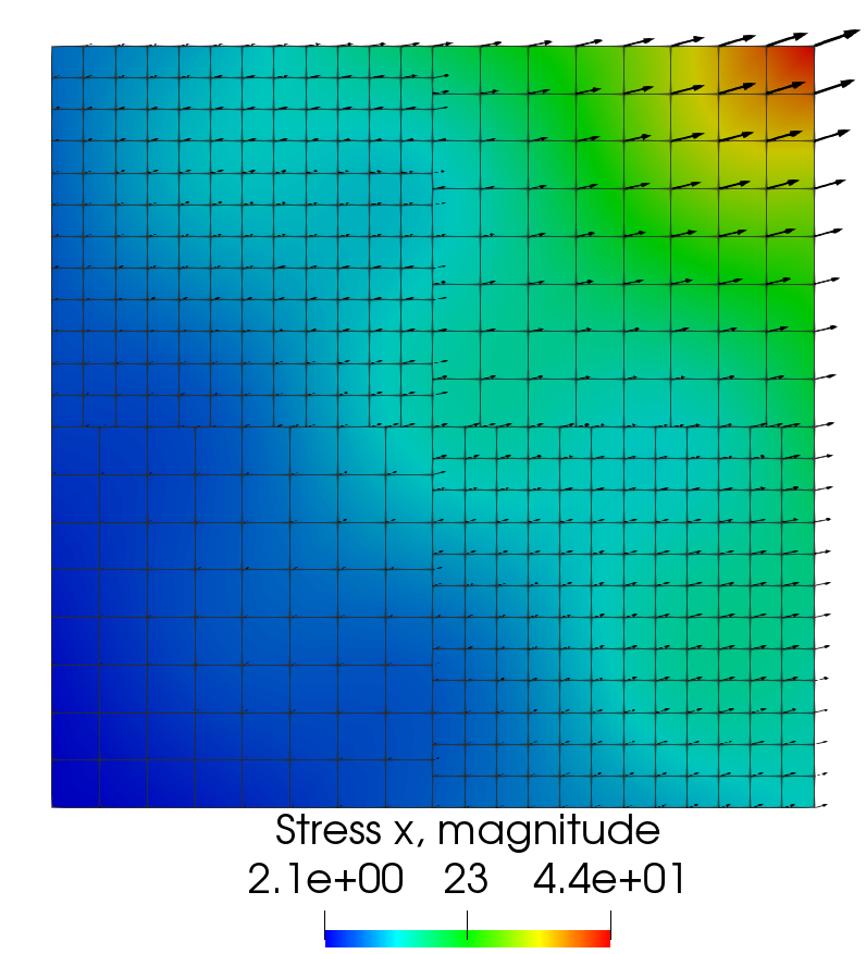
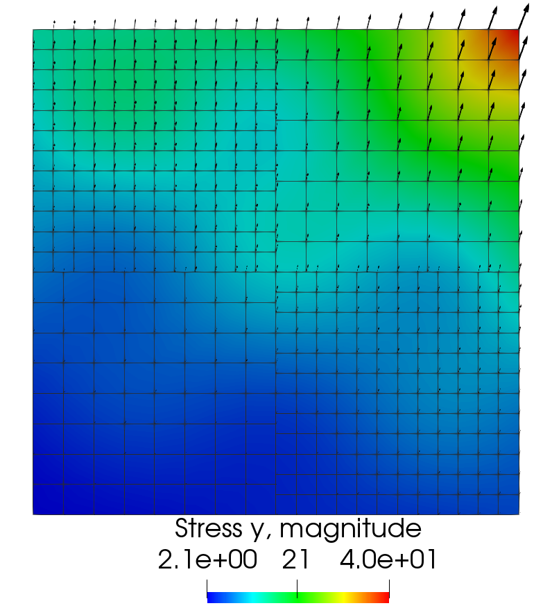
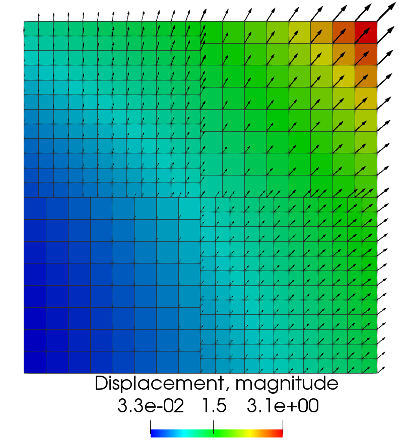
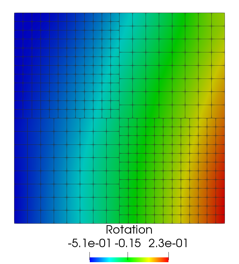
Figure 1: Computed solution for Example 1, $h=1/16$.

5.2 Example 2

In the second example, we solve a problem with discontinuous Lamé parameters. We choose $\lambda=\mu=1$ for $0<x<0.5$ and $\lambda=\mu=10$ for $0.5<x<1$. The solution

$$u=\begin{pmatrix}x^{2}y^{3}-x^{2}y^{3}\sin(\pi x)\\ x^{2}y^{3}-x^{2}y^{3}\sin(\pi x)\end{pmatrix}$$

is chosen to be continuous with continuous normal stress and rotation at $x=0.5$. Convergence rates are provided in Tables 4 and 5. The computed solution is plotted in Figure 2.

	$\|\sigma-\sigma_{h}\|$		$\|\operatorname{div}(\sigma-\sigma_{h})\|$		$\|u-u_{h}\|$		$\|\mathcal{P}_{h}u-u_{h}\|$		$\|\gamma-\gamma_{h}\|$		$\|u-\lambda_{H}\|_{a}$		CG iter.
$h$	error	rate	error	rate	error	rate	error	rate	error	rate	error	rate	#	rate
1/4	2.02E-1	-	5.64E-1	-	4.57E-1	-	2.54E-1	-	4.08E-1	-	5.01E-1	-	45	-
1/8	5.43E-2	1.9	2.98E-1	0.9	2.12E-1	1.1	7.14E-2	1.8	1.04E-1	2.0	1.33E-1	1.9	61	-0.4
1/16	1.37E-2	2.0	1.51E-1	1.0	1.04E-1	1.0	1.84E-2	2.0	2.60E-2	2.0	3.25E-2	2.0	85	-0.5
1/32	3.42E-3	2.0	7.58E-2	1.0	5.15E-2	1.0	4.63E-3	2.0	6.47E-3	2.0	7.83E-3	2.1	122	-0.5
1/64	8.53E-4	2.0	3.79E-2	1.0	2.57E-2	1.0	1.16E-3	2.0	1.61E-3	2.0	1.88E-3	2.1	170	-0.5
1/128	2.13E-4	2.0	1.90E-2	1.0	1.28E-2	1.0	2.90E-4	2.0	4.02E-4	2.0	4.55E-4	2.1	252	-0.6
1/256	5.33E-5	2.0	9.48E-3	1.0	6.42E-3	1.0	7.25E-5	2.0	1.00E-4	2.0	1.10E-4	2.0	354	-0.5

Table 4: Numerical errors, convergence rates, and number of CG iterations with discontinuous quadratic mortars ($m=2$) for Example 2.

	$\|\sigma-\sigma_{h}\|$		$\|\operatorname{div}(\sigma-\sigma_{h})\|$		$\|u-u_{h}\|$		$\|\mathcal{P}_{h}u-u_{h}\|$		$\|\gamma-\gamma_{h}\|$		$\|u-\lambda_{H}\|_{a}$		CG iter.
$h$	error	rate	error	rate	error	rate	error	rate	error	rate	error	rate	#	rate
1/4	2.04E-1	-	5.64E-1	-	4.58E-1	-	2.54E-1	-	4.04E-1	-	5.11E-1	-	52	-
1/16	1.37E-2	1.9	1.51E-1	1.0	1.04E-1	1.1	1.85E-2	1.9	2.62E-2	2.0	3.27E-2	2.0	83	-0.3
1/64	8.68E-4	2.0	3.79E-2	1.0	2.57E-2	1.0	1.16E-3	2.0	1.71E-3	2.0	1.90E-3	2.1	135	-0.4
1/256	5.51E-5	2.0	9.48E-3	1.0	6.42E-3	1.0	7.23E-5	2.0	1.15E-4	2.0	1.19E-4	2.0	211	-0.3

Table 5: Numerical errors, convergence rates, and number of CG iterations with discontinuous cubic mortars ($m=3$) for Example 2.

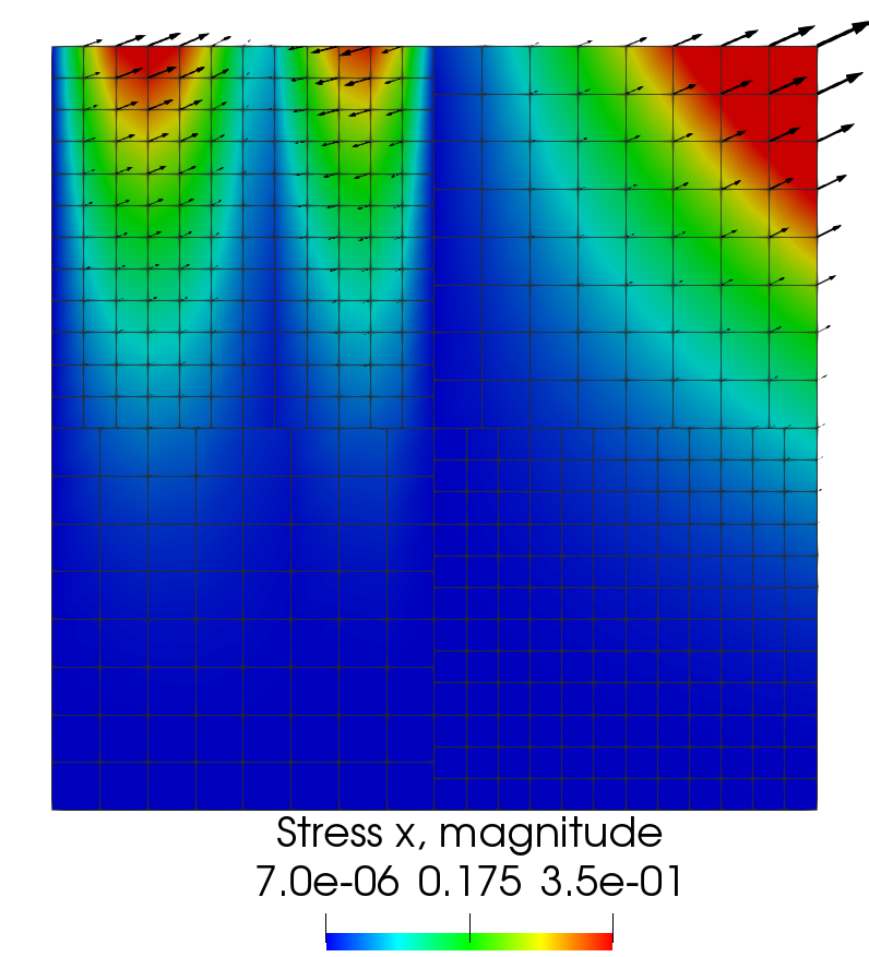
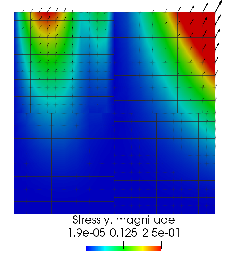
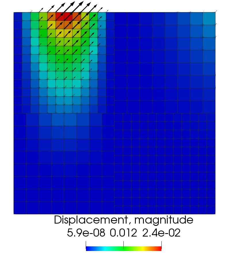
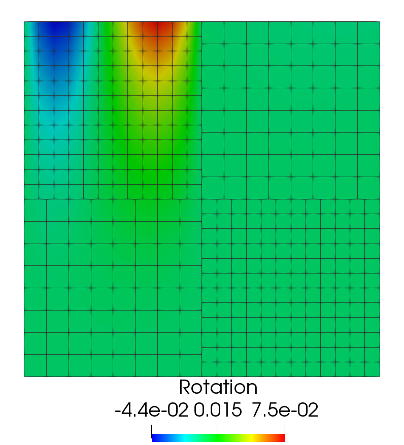
Figure 2: Computed solution for Example 2, $h=1/16$.

5.3 Example 3

In third example we study a three-dimensional problem, which models simultaneous twisting and compression (about $x$-axis) of the unit cube. The displacement solution is

$$u=\begin{pmatrix}-0.1(e^{x}-1)\sin(\pi x)\sin(\pi y)\\ -(e^{x}-1)(y-\cos(\frac{\pi}{12})(y-0.5)+\sin(\frac{\pi}{12})(z-0.5)-0.5)\\ -(e^{x}-1)(z-\sin(\frac{\pi}{12})(y-0.5)-\cos(\frac{\pi}{12})(z-0.5)-0.5)\end{pmatrix}.$$

The Lamé parameters are $\lambda=\mu=100$. The computed relative errors, convergence rates, and the number of interface iterations are shown in Table 6. We note that the mortar displacement exhibits slightly higher convergence rate than the theoretical rate. The computed solution is plotted in Figure 3.

	$\|\sigma-\sigma_{h}\|$		$\|\operatorname{div}(\sigma-\sigma_{h})\|$		$\|u-u_{h}\|$		$\|\mathcal{P}_{h}u-u_{h}\|$		$\|\gamma-\gamma_{h}\|$		$\|u-\lambda_{H}\|_{a}$		CG iter.
$h$	error	rate	error	rate	error	rate	error	rate	error	rate	error	rate	#	rate
1/4	2.71E-1	-	3.85E-1	-	2.60E-1	-	3.87E-2	-	1.37E-1	-	2.80E-2	-	21	-
1/8	1.22E-1	1.2	1.96E-1	1.0	1.31E-1	1.0	8.40E-3	2.2	6.83E-2	1.0	7.99E-3	1.8	37	-0.8
1/16	5.79E-2	1.1	9.87E-2	1.0	6.54E-2	1.0	2.09E-3	2.0	3.41E-2	1.0	2.39E-3	1.7	56	-0.6
1/32	2.82E-2	1.0	4.94E-2	1.0	3.27E-2	1.0	5.31E-4	2.0	1.71E-2	1.0	8.18E-4	1.6	80	-0.5

Table 6: Numerical errors, convergence rates, and number of CG iterations with discontinuous linear mortars ($m=1$) for Example 3.

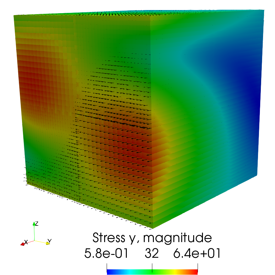
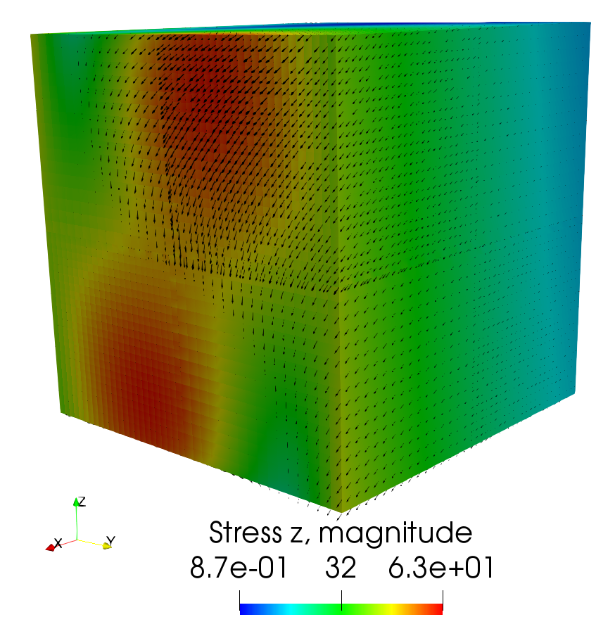
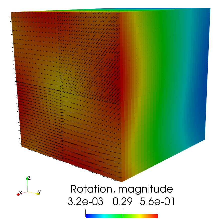
Figure 3: Computed solution for Example 3, $h=1/32$.

5.4 Example 4

In this example we study the dependence of the number of CG iterations on the number of subdomains used for solving the problem. We consider the same test case as in Example 1 with discontinuous quadratic mortars, but solve the problem using $2\times 2$, $4\times 4$ and $8\times 8$ subdomain partitionings. We report the number of CG iterations in Table 7. For the sake of space and clarity we do not show the rate of growth for each refinement step, but only the average values. For each fixed domain decomposition (each column) we observe growth of $\mathcal{O}(h^{-0.5})$ as the grids are refined, confirming condition number $\kappa=\mathcal{O}(h^{-1})$, as in the previous examples with $2\times 2$ decompositions. Considering each row, we observe that the number of CG iterations grows as the subdomain size $A$ decreases with rate $\mathcal{O}(A^{-0.5})$, implying that $\kappa=\mathcal{O}(A^{-1})$. This is expected for an algorithm without a coarse solve preconditioner [43]. This issue will be addressed in forthcoming work.

$h$	$2\times 2$	$4\times 4$	$8\times 8$	Rate
1/16	48	67	94	$\mathcal{O}(A^{-0.5})$
1/32	63	94	118	$\mathcal{O}(A^{-0.5})$
1/64	96	133	167	$\mathcal{O}(A^{-0.4})$
1/128	136	189	230	$\mathcal{O}(A^{-0.4})$
1/256	194	267	340	$\mathcal{O}(A^{-0.4})$
Rate	$\mathcal{O}(h^{-0.5})$	$\mathcal{O}(h^{-0.5})$	$\mathcal{O}(h^{-0.5})$

Table 7: Number of CG iterations for Example 4.

5.5 Example 5

In the last example we test the efficiency of the multiscale stress basis (MSB) technique outlined in the previous section. With no MSB the total number of solves is $\#\text{CG iter.}+3$, one for each CG iteration plus one solve for the right hand side of type (3.5)–(3.7), one for the initial residual and one to recover the final solution. On the other hand, the method with MSB requires $\text{dim}(\Lambda_{H})+3$ solves, hence its use is advantageous when $\text{dim}(\Lambda_{h})<\#\text{CG iter.}$, that is when the mortar grid is relatively coarse.

We use a heterogeneous porosity field from the Society of Petroleum Engineers (SPE) Comparative Solution Project2. The computation domain is $\Omega=(0,1)^{2}$ with a fixed rectangular $128\times 128$ grid. The left and right boundary conditions are $u=(0.1,0)^{T}$ and $u=(0,0)^{T}$. Zero normal stress, $\sigma\,n=0$, is specified on the top and bottom boundaries. Given the porosity $\phi$, the Young’s modulus is obtained from the relation [33] $E=10^{2}\left(1-\frac{\phi}{c}\right)^{2.1}$, where the constant $c=0.5$ refers to the porosity at which the effective Young’s modulus becomes zero. The choice of this constant is based on the properties of the deformable medium, see [33] for details. The resulting Young’s modulus field is shown in Figure 4.

A comparison between the fine scale solution and the multiscale solution with $8\times 8$ subdomains and a single cubic mortar per interface is shown in Figure 4. We observe that the two solutions are very similar and that the multiscale solution captures the heterogeneity very well, even for this very coarse mortar space. In Table 8 we compare the cost of using MSB and not using MSB for several choices of mortar grids. We report the number of solves per subdomain, which is the dominant computational cost. We conclude that for cases with relatively coarse mortar grids, the MSB technique requires significantly fewer subdomain solves, resulting in faster computations. Moreover, as evident from the last row in Table 8, computing the fine scale solution is significantly more expensive than computing the multiscale solution.

Mortar type	$H$	# Solves, no MSB	# Solves, MSB
Quadratic	1/8	180	27
Cubic	1/8	173	35
Quadratic	1/16	219	51
Cubic	1/16	250	67
Linear (fine scale solution)	1/128	295	195

Table 8: Number of subdomain solves for Example 5.

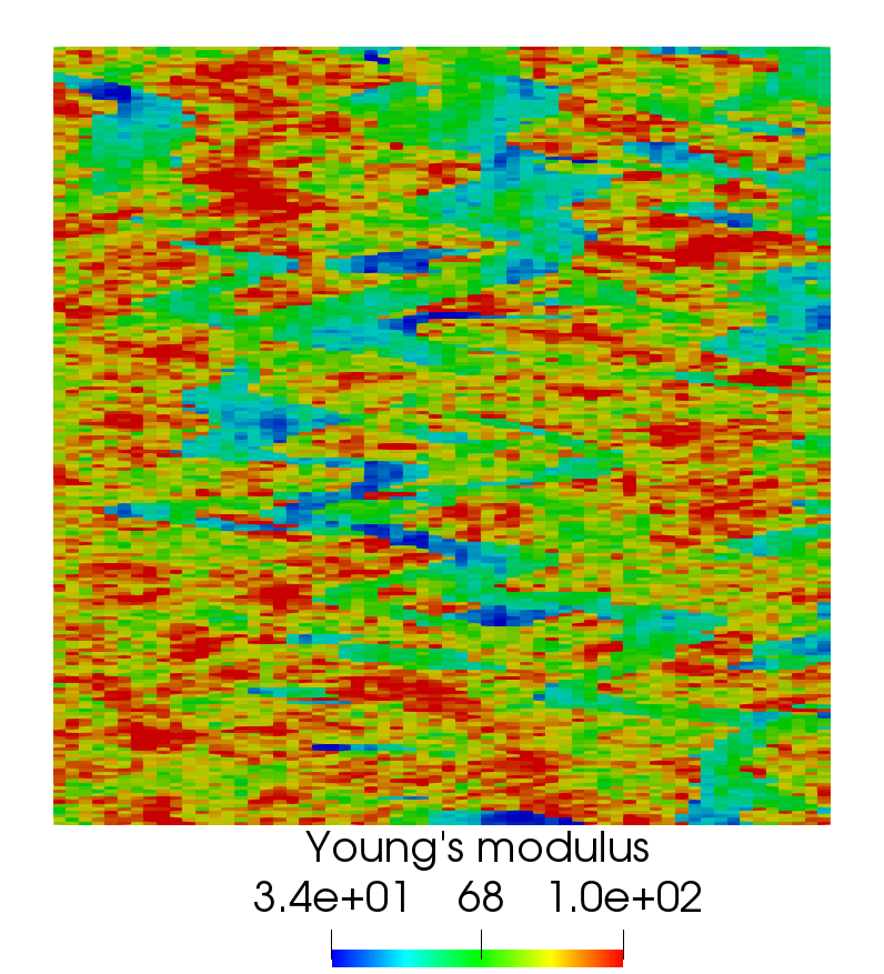
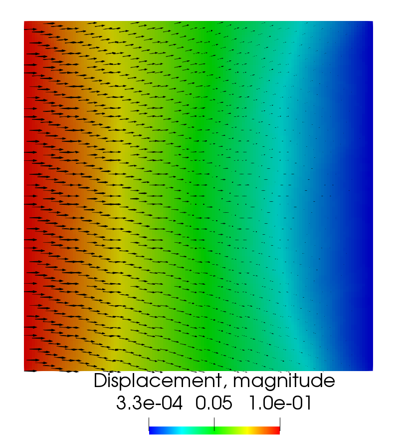
Figure 4: Example 5, Young’s modulus, fine scale stress and displacement, and multiscale stress and displacement with cubic mortars, $H=1/8$.

References

• [1] M. Amara and J. M. Thomas, Equilibrium finite elements for the linear elastic problem, Numer. Math., 33 (1979), pp. 367–383.
• [2] I. Ambartsumyan, E. Khattatov, J. Nordbotten, and I. Yotov, A multipoint stress mixed finite element method for elasticity I: Simplicial grids. Preprint.
• [3] I. Ambartsumyan, E. Khattatov, J. Nordbotten, and I. Yotov, A multipoint stress mixed finite element method for elasticity II: Quadrilateral grids. Preprint.
• [4] T. Arbogast, L. C. Cowsar, M. F. Wheeler, and I. Yotov, Mixed finite element methods on nonmatching multiblock grids, SIAM J. Numer. Anal., 37 (2000), pp. 1295–1315.
• [5] T. Arbogast, G. Pencheva, M. F. Wheeler, and I. Yotov, A multiscale mortar mixed finite element method, Multiscale Model. Simul., 6 (2007), pp. 319–346.
• [6] D. Arndt, W. Bangerth, D. Davydov, T. Heister, L. Heltai, M. Kronbichler, M. Maier, J.-P. Pelteret, B. Turcksin, and D. Wells, The deal.II library, version 8.5, J. Numer. Math., 25 (2017), pp. 137–146.
• [7] D. N. Arnold, G. Awanou, and W. Qiu, Mixed finite elements for elasticity on quadrilateral meshes, Adv. Comput. Math., 41 (2015), pp. 553–572.
• [8] D. N. Arnold, F. Brezzi, and J. Douglas, Jr., PEERS: a new mixed finite element for plane elasticity, Japan J. Appl. Math., 1 (1984), pp. 347–367.
• [9] D. N. Arnold, R. S. Falk, and R. Winther, Mixed finite element methods for linear elasticity with weakly imposed symmetry, Math. Comp., 76 (2007), pp. 1699–1723.
• [10] D. N. Arnold and J. J. Lee, Mixed methods for elastodynamics with weak symmetry, SIAM J. Numer. Anal., 52 (2014), pp. 2743–2769.
• [11] G. Awanou, Rectangular mixed elements for elasticity with weakly imposed symmetry condition, Adv. Comput. Math., 38 (2013), pp. 351–367.
• [12] D. Boffi, F. Brezzi, and M. Fortin, Reduced symmetry elements in linear elasticity, Commun. Pure Appl. Anal., 8 (2009), pp. 95–121.
• [13] F. Brezzi and M. Fortin, Mixed and hybrid finite element methods, vol. 15 of Springer Series in Computational Mathematics, Springer-Verlag, New York, 1991.
• [14] P. G. Ciarlet, The finite element method for elliptic problems, vol. 40 of Classics in Applied Mathematics, Society for Industrial and Applied Mathematics, Philadelphia, PA, 2002.
• [15] B. Cockburn, J. Gopalakrishnan, and J. Guzmán, A new elasticity element made for enforcing weak stress symmetry, Math. Comp., 79 (2010), pp. 1331–1349.
• [16] L. C. Cowsar, J. Mandel, and M. F. Wheeler, Balancing domain decomposition for mixed finite elements, Math. Comp., 64 (1995), pp. 989–1015.
• [17] M. Dauge, Elliptic boundary value problems on corner domains, vol. 1341 of Lecture Notes in Mathematics, Springer-Verlag, Berlin, 1988. Smoothness and asymptotics of solutions.
• [18] Y. Efendiev, J. Galvis, and T. Y. Hou, Generalized multiscale finite element methods (GMsFEM), J. Comput. Phys., 251 (2013), pp. 116–135.
• [19] C. Farhat and F.-X. Roux, A method of finite element tearing and interconnecting and its parallel solution algorithm, Internat. J. Numer. Methods Engrg., 32 (1991), pp. 1205–1227.
• [20] A. Fritz, S. Hüeber, and B. I. Wohlmuth, A comparison of mortar and Nitsche techniques for linear elasticity, Calcolo, 41 (2004), pp. 115–137.
• [21] J. Galvis and M. Sarkis, Non-matching mortar discretization analysis for the coupling Stokes-Darcy equations, Electron. Trans. Numer. Anal., 26 (2007), pp. 350–384.
• [22] B. Ganis and I. Yotov, Implementation of a mortar mixed finite element method using a multiscale flux basis, Comput. Methods Appl. Mech. Engrg., 198 (2009), pp. 3989–3998.
• [23] V. Girault, G. V. Pencheva, M. F. Wheeler, and T. M. Wildey, Domain decomposition for linear elasticity with DG jumps and mortars, Comput. Methods Appl. Mech. Engrg., 198 (2009), pp. 1751–1765.
• [24] R. Glowinski and M. F. Wheeler, Domain decomposition and mixed finite element methods for elliptic problems, in First International Symposium on Domain Decomposition Methods for Partial Differential Equations, R. G. et al., ed., SIAM, Philadelphia, 1988, pp. 144–172.
• [25] P. Goldfeld, L. F. Pavarino, and O. B. Widlund, Balancing Neumann-Neumann preconditioners for mixed approximations of heterogeneous problems in linear elasticity, Numer. Math., 95 (2003), pp. 283–324.
• [26] J. Gopalakrishnan and J. Guzmán, A second elasticity element using the matrix bubble, IMA J. Numer. Anal., 32 (2012), pp. 352–372.
• [27] P. Grisvard, Elliptic problems in nonsmooth domains, vol. 69 of Classics in Applied Mathematics, Society for Industrial and Applied Mathematics (SIAM), Philadelphia, PA, 2011.
• [28] P. Hauret and P. Le Tallec, A discontinuous stabilized mortar method for general 3D elastic problems, Comput. Methods Appl. Mech. Engrg., 196 (2007), pp. 4881–4900.
• [29] C. T. Kelley, Iterative methods for linear and nonlinear equations, vol. 16 of Frontiers in Applied Mathematics, Society for Industrial and Applied Mathematics, Philadelphia, 1995.
• [30] H. H. Kim, A BDDC algorithm for mortar discretization of elasticity problems, SIAM J. Numer. Anal., 46 (2008), pp. 2090–2111.
• [31] H. H. Kim, A FETI-DP formulation of three dimensional elasticity problems with mortar discretization, SIAM J. Numer. Anal., 46 (2008), pp. 2346–2370.
• [32] A. Klawonn and O. B. Widlund, A domain decomposition method with Lagrange multipliers for linear elasticity, in Eleventh International Conference on Domain Decomposition Methods (London, 1998), Augsburg, 1999, pp. 49–56.
• [33] J. Kovacik, Correlation between Young’s modulus and porosity in porous materials, J. Mater. Sci. Lett., 18 (1999), pp. 1007–1010.
• [34] J.-L. Lions and E. Magenes, Non-homogeneous boundary value problems and applications. Vol. I, Springer-Verlag, New York-Heidelberg, 1972.
• [35] T. P. Mathew, Domain decomposition and iterative refinement methods for mixed finite element discretizations of elliptic problems, PhD thesis, Courant Institute of Mathematical Sciences, New York University, 1989. Tech. Rep. 463.
• [36] L. F. Pavarino, O. B. Widlund, and S. Zampini, BDDC preconditioners for spectral element discretizations of almost incompressible elasticity in three dimensions, SIAM J. Sci. Comput., 32 (2010), pp. 3604–3626.
• [37] G. Pencheva and I. Yotov, Balancing domain decomposition for mortar mixed finite element methods, Numer. Linear Algebra Appl., 10 (2003), pp. 159–180.
• [38] M. Peszyńska, M. F. Wheeler, and I. Yotov, Mortar upscaling for multiphase flow in porous media, Comput. Geosci., 6 (2002), pp. 73–100.
• [39] A. Quarteroni and A. Valli, Domain Decomposition Methods for Partial Differential equations, Clarendon Press, Oxford, 1999.
• [40] J. E. Roberts and J.-M. Thomas, Mixed and hybrid methods, in Handbook of numerical analysis, Vol. II, Handb. Numer. Anal., II, North-Holland, Amsterdam, 1991, pp. 523–639.
• [41] L. R. Scott and S. Zhang, Finite element interpolation of nonsmooth functions satisfying boundary conditions, Math. Comput., 54 (1990), pp. 483–493.
• [42] R. Stenberg, A family of mixed finite elements for the elasticity problem, Numer. Math., 53 (1988), pp. 513–538.
• [43] A. Toselli and O. Widlund, Domain decomposition methods—algorithms and theory, vol. 34 of Springer Series in Computational Mathematics, Springer-Verlag, Berlin, 2005.
• [44] D. Vassilev, C. Wang, and I. Yotov, Domain decomposition for coupled Stokes and Darcy flows, Comput. Methods Appl. Mech. Engrg., 268 (2014), pp. 264–283.
• [45] M. F. Wheeler, G. Xue, and I. Yotov, A multiscale mortar multipoint flux mixed finite element method, ESAIM Math. Model. Numer. Anal., 46 (2012), pp. 759–796.