A Further Test of Lorentz Violation from the Rest-Frame Spectral Lags of Gamma-Ray Bursts

Abstract

Lorentz invariance violation (LIV) can manifest itself by an energy-dependent vacuum dispersion of light, which leads to arrival-time differences of photons with different energies originating from the same astronomical source. The spectral lags of gamma-ray bursts (GRBs) have been widely used to investigate the possible LIV effect. However, all current investigations used lags extracted in the observer frame only. In this work, we present, for the first time, an analysis of the LIV effect and its redshift dependence in the cosmological rest frame. Using a sample of 56 GRBs with known redshifts, we obtain a robust limit on LIV by fitting their rest-frame spectral lag data both using a maximization of the likelihood function and a minimum $\chi^{2}$ statistic. Our analysis indicates that there is no evidence of LIV. Additionally, we test the LIV in different redshift ranges by dividing the full sample into four redshift bins. We also find no evidence for the redshift variation of the LIV effect.

1. Introduction

Lorentz invariance is a fundamental symmetry of space-time in modern physics. However, many Quantum Gravity (QG) theories, which attempt to unify general relativity and quantum mechanics, predict the existence of deviations from Lorentz symmetry at the Planck energy scale ($E_{\rm Pl}=\sqrt{\hbar c^{5}/G}\simeq 1.22\times 10^{19}$ GeV; Pavlopoulos 1967; Kostelecký & Samuel 1989; Kostelecký & Potting 1991, 1995; Mattingly 2005; Bluhm 2005; Amelino-Camelia 2013; Tasson 2014). As a consequence of Lorentz invariance violation (LIV), the speed of light in a vacuum would have an energy dependence, the so-called vacuum dispersion (Amelino-Camelia et al., 1997; Kostelecký & Mewes, 2008; Ellis et al., 2008, 2011). The energy scale for LIV, $E_{\rm QG}$, could therefore be constrained by comparing the arrival-time differences of photons with different energies emitted simultaneously from the same source (Amelino-Camelia et al., 1998; Ellis & Mavromatos, 2013).

Because of the high-energy extent of their emission, their large cosmological distances, and their fast variabilities, gamma-ray bursts (GRBs) have been deemed as the most promising sources for searching for LIV-induced vacuum dispersion (Amelino-Camelia et al., 1998; Jacob & Piran, 2007; Amelino-Camelia & Smolin, 2009; Amelino-Camelia, 2013; Wei et al., 2016). To date, various limits on LIV have been obtained by studying the dispersion of light in observations of individual GRBs or a large sample of GRBs (Amelino-Camelia et al. 1998; Coleman & Glashow 1999; Schaefer 1999; Boggs et al. 2004; Pavlopoulos 2005; Kahniashvili et al. 2006; Jacob & Piran 2008; Abdo et al. 2009b, a; Xiao & Ma 2009; Shao et al. 2010; Chang et al. 2012; Nemiroff et al. 2012; Kostelecký & Mewes 2013; Vasileiou et al. 2013; Zhang & Ma 2015; Xu & Ma 2016, see also Kostelecký & Russell 2011; Liberati 2013 and summary constraints for LIV therein). Although these limits on LIV have reached high precision, most were obtained by relying on the rough time lag of a single highest-energy photon. Performing a search for LIV using the true time lags of high-quality and high-energy light curves in different energy multi-photon bands is therefore crucial. Furthermore, the method of the arrival-time difference used for testing LIV is tempered by our ignorance concerning the intrinsic time delay that depends on the unknown emission mechanism of GRBs. Most previous studies concentrated on the time delay induced by LIV while neglecting the intrinsic time delay, which would impact the reliability of the resulting constraints on LIV. Most recently, however, Wei et al. (2017a, b) provided some solutions to disentangle the intrinsic time delay problem. They first proposed that the only burst GRB 160625B so far with a well-defined transition from positive to negative spectral lags provides a good opportunity to distinguish the possible LIV effect from any source-intrinsic time delay in the emission of photons of different energy bands. By fitting the true multi-photon spectral-lag data of GRB 160625B, they obtained both a reasonable formulation of the intrinsic energy-dependent time delay and robust limits on the QG energy scale and the Lorentz-violating coefficients of the Standard-Model Extension.

In order to identify an effect as radical as Lorentz violation, statistical and possible systematic uncertainties must be minimized. For this purpose, Ellis et al. (2000, 2003, 2006) developed a method for analyzing a statistical sample of 35 GRBs with different redshifts, rather than a single source. For each GRB, Ellis et al. (2006) looked for the spectral time-lag in the light curves recorded in the selected observer-frame energy bands 25–55 and 115–320 keV. This technique has the advantage that it can extract the spectral lags of broad light curves in different energy multi-photon bands. In their analysis, the observed time lag was formulated in terms of linear regression where the slope corresponds to the LIV effect and the intercept denotes the intrinsic time delay at the source. Assuming the concordance $\Lambda$CDM model as the background cosmology, they found a weak evidence for LIV and obtained a robust lower limit of $E_{\rm QG}\geq 1.4\times 10^{16}$ GeV (Ellis et al., 2006). Subsequently, Biesiada & Piórkowska (2009); Pan et al. (2015) applied this procedure to different cosmological models, finding the conclusion is independent of the background cosmology. We note that the spectral lags of GRBs used for testing LIV were extracted between two fixed energy bands in the observer frame (Ellis et al., 2006). Due to the redshift dependence of GRBs, however, these two energy bands can correspond to a different pair of energy bands in the rest frame (Ukwatta et al., 2012), thus potentially introducing an energy dependence to the extracted spectral lag and/or an extra uncertainty to the resulting constraints on LIV. Ukwatta et al. (2012) studied the correlation between observer-frame lags and rest-frame lags for the same sample of 31 GRBs (see Figure 3 of Ukwatta et al. (2012)). They showed that there is a large scatter in this correlation, implying the observer-frame lag does not directly represent the rest-frame lag. In other words, the observer-frame lags would be strongly biased since they simply recorded different pairs of the intrinsic light curves. This can be resolved by choosing two appropriate energy bands fixed in the rest frame and estimating the observed lag for two projected energy bands by the relation $E_{\rm obs}=E_{\rm rest}/(1+z)$, where $E_{\rm obs}$ and $E_{\rm rest}$ are the photon energy measured in the observer and the rest frame, respectively. It actually means that the energy-dependent effect can be removed in this way. However, no one has made systematical research on the LIV effect using the spectral lags extracted in the rest frame.

Recently, Bernardini et al. (2015) investigated the rest-frame spectral lags of the complete sample of 56 bright GRBs observed by Swift/Burst Alert Telescope (BAT). For each GRB, they extracted mask-weighted, background-subtracted light curves for two observer-frame energy bands corresponding to the fixed rest-frame energy bands 100–150 and 200–250 keV. These two particular rest-frame energy bands were selected so that after transforming to the observer frame (i.e., $[100$–$150]/(1+z)$ and $[200$–$250]/(1+z)$ keV) they still lie in the energy range of the BAT instrument ($\sim[15$–$200]$ keV). For each light-curve pairs, they estimated the time lag and the associated uncertainty through a discrete cross-correlation function fitted with an asymmetric Gaussian function (Bernardini et al., 2015).

In this work, we make use of the rest-frame spectral lags from 56 Swift GRBs presented in Bernardini et al. (2015) for the first time to study the possible LIV effect. Compared with previous works, which relied on using the observer-frame lags, our present work can remove the problem associated with the energy dependence of the extracted spectral lags, and then obtain reliable constraints on LIV. On the other hand, since the GRBs in the sample of Bernardini et al. (2015) cover a wide redshift range $z\in[0.35$–$5.47]$, they also enable us to test the LIV in different redshift ranges for the first time. To test whether the LIV effect varies with the cosmological redshift, in this work we separate the sample of 56 GRBs into four redshift bins. That is, we sort the GRBs by their redshift measurements, and divide them into four groups with redshifts from low to high, each group containing 14 GRBs. We then perform the linear fit to each group and calculate the mean redshift, and check whether the values of the linear terms that encoded the LIV effect evolve with redshift.

The outline of this paper is as follows. In Section 2, we give an overview of the LIV formalism. In Section 3, we describe the sample at our disposal and our method of analysis. The resulting constraints on LIV and its redshift dependence from the rest-frame spectral lags of GRBs are presented in Section 4. Finally, a brief discussion and conclusion are drawn in Section 5.

2. Formalism

As mentioned above, the speed of light would become energy-dependent in a vacuum due to the LIV effect. The modified dispersion relation of photons can be described using the leading term of the Taylor series expansion in the form

$$E^{2}\simeq p^{2}c^{2}\left[1-s_{\pm}\left(\frac{pc}{E_{{\rm QG},n}}\right)^{n}\right]\;,$$ (1)

which corresponds to a modified photon velocity

$$v(E)=\frac{\partial E}{\partial p}\approx c\left[1-s_{\pm}\frac{n+1}{2}\left(\frac{E}{E_{{\rm QG},n}}\right)^{n}\right]\;,$$ (2)

where $E_{\rm QG}$ represents the QG energy scale, the $n$th-order expansion of the leading term stands for linear ($n=1$) or quadratic ($n=2$) energy dependence, and $s_{\pm}=\pm 1$ is the “sign of LIV” (Amelino-Camelia & Piran, 2001). $s_{\pm}=+1$ ($s_{\pm}=-1$) corresponds to a decrease (an increase) in photon speed with an increasing photon energy. For the sake of being comparable with the results of Ellis et al. (2006) and because the data used in this study are not sensitive to higher order terms, here we only consider the $n=1$ case, and moreover we assume the sign parameter $s_{\pm}=-1$ in the formula. Photons with higher energies would travel faster than those with lower energies in the case of $s_{\pm}=-1$, which predicts a positive spectral lag due to LIV, i.e., $\Delta t_{\rm LIV}>0$.

Because of the spectral dispersion, two photons with different observer-frame energies ($E_{h}>E_{l}$) arising from the same source would arrive at the observer with a time delay. Taking into consideration the cosmological expansion, the LIV-induced time delay can be expressed by (Jacob & Piran, 2008; Zhang & Ma, 2015)

$$\Delta t_{\rm LIV} =\frac{E_{h}-E_{l}}{H_{0}E_{\rm QG}}\int_{0}^{z}\frac{(1+z^{\prime}){\rm d}z^{\prime}}{h(z^{\prime})}$$ (3)

$$=\frac{E^{\prime}_{h}/(1+z)-E^{\prime}_{l}/(1+z)}{H_{0}E_{\rm QG}}\int_{0}^{z}\frac{(1+z^{\prime}){\rm d}z^{\prime}}{h(z^{\prime})}\;,$$

where $E^{\prime}_{h}=E_{h}(1+z)$ and $E^{\prime}_{l}=E_{l}(1+z)$ are the rest-frame energies, respectively. Also, $h(z)=\sqrt{\Omega_{\rm m}(1+z)^{3}+\Omega_{\Lambda}}$ is the dimensionless Hubble expansion rate at $z$, where the standard flat $\Lambda$CDM model with parameters $H_{0}=67.8$ km $\rm s^{-1}$ $\rm Mpc^{-1}$, $\Omega_{\rm m}=0.308$, and $\Omega_{\Lambda}=1-\Omega_{\rm m}$ is adopted (Planck Collaboration et al., 2016).

Due to the fact that the LIV-induced time delay $\Delta t_{\rm LIV}$ is likely to be accompanied by an unknown intrinsic time lag caused by unknown properties of the source (Ellis et al., 2006; Biesiada & Piórkowska, 2009), we take this possibility into account by fitting the observed time lag with the inclusion of a term $\langle b\rangle$ specified in the rest-frame of the source, as Ellis et al. (2006) did in their treatment. Therefore, the observed arrival time delays consist of two terms

$$\Delta t_{\rm obs}=\Delta t_{\rm LIV}+\langle b\rangle(1+z)\;,$$ (4)

reflecting the possible LIV effect and intrinsic source effect, respectively. Then we re-express Equation (4) as a linear function in the form:

$$\frac{\Delta t_{\rm obs}}{1+z}=a_{\rm LIV}K+\langle b\rangle,$$ (5)

where

$$K=\frac{1}{(1+z)^{2}}\int_{0}^{z}\frac{(1+z^{\prime}){\rm d}z^{\prime}}{h(z^{\prime})}$$ (6)

is a function of the redshift, and

$$a_{\rm LIV}=\frac{E^{\prime}_{h}-E^{\prime}_{l}}{H_{0}E_{\rm QG}}$$ (7)

is the slope in $K$ which is related to the scale of Lorentz violation, whereas the intercept $\langle b\rangle$ denotes the average effect of the intrinsic time lags of different pulses internal to the GRB. Note that intrinsic time lags apply most strictly between individual pulses internal to GRBs (see Kocevski & Liang 2003; Norris et al. 2005). As shown by Hakkila & Giblin (2004) and Zhang (2012), different pulses inside the same GRB can have different intrinsic lags. We adopt the view that using a single time lag $\langle b\rangle$ for an entire GRB would be sufficient to demonstrate the essential point (Ellis et al., 2006; Biesiada & Piórkowska, 2009; Pan et al., 2015), but this should be understood to be a statistical average over the different lags of different pulses internal to the GRB.

Additionally, it should be pointed out that the intrinsic time lags are not generally a single time offset between GRB light curves in different energy bands. As described by Norris (2002), the time lag is a cross correlation between light curves of the same pulse at two different energy bands. This cross correlation is not caused, typically, by a single time offset true at all times during the pulse, but rather a variable time offset that increases as the pulse progresses. This has been shown in some detail by Nemiroff (2000) for GRB 930214C, and more generally by Hakkila & Nemiroff (2009). As such, the total measured time offset is typically zero at the beginning of each pulse (the Pulse Start Conjecture, Nemiroff 2000, 2012; Hakkila & Nemiroff 2009), but may even be on the order of the duration of the pulse near the temporal conclusion of the pulse. It would be more accurate to consider pulses as starting at the same time at all energies but being increasingly stretched out at lower energies, typically. Therefore, any LIV-induced time lag would act in a fundamentally different manner than an intrinsic time lag, as measured. LIV-induced time lags would really be a single time offset, on the average, between GRB photons at different energies. LIV-induced time lags between energy bands would be the same at all times in the light curves of GRB pulses, whereas intrinsic time lags would differ. In summary, the intrinsic time lags are attributes of the later parts of GRB pulses, here we simply use a single average lag $\langle b\rangle$ for an entire GRB.

Table 1Data on spectral time lags for 56 GRBs with known redshifts. The values of $z$, $\Delta t_{\rm obs}$, and the corresponding left ($\sigma_{\rm l}$) and right ($\sigma_{\rm r}$) uncertainties of $\Delta t_{\rm obs}$ are collected from Bernardini et al. (2015).

GRB name	$z$	$\Delta t_{\rm obs}$ (ms)	$\sigma_{\rm l}$ (ms)	$\sigma_{\rm r}$ (ms)
050318	1.44	-13.66	184.88	218.76
050401	2.90	285.19	59.05	59.14
050525A	0.61	54.72	25.42	25.59
050802	1.71	555.80	386.11	395.90
050922C	2.20	162.52	74.74	79.50
060206	4.05	252.40	85.65	88.18
060210	3.91	349.99	233.64	237.12
060306	1.55	42.56	51.17	53.73
060814	1.92	-100.01	138.04	138.73
060908	1.88	230.04	169.95	175.42
060912A	0.94	-7.09	82.58	83.49
060927	5.47	14.26	111.90	111.69
061007	1.26	27.05	25.42	26.88
061021	0.35	-603.94	416.22	403.94
061121	1.31	28.36	20.02	20.25
061222A	2.09	6.07	145.67	139.01
070306	1.50	-213.78	290.08	281.92
070521	1.35	40.20	39.51	39.07
071020	2.15	48.47	10.70	10.24
071117	1.33	258.54	41.21	42.58
080319B	0.94	30.29	21.67	19.18
080319C	1.95	217.82	168.48	171.20
080413B	1.10	96.00	61.91	59.56
080430	0.77	44.04	564.87	634.35
080603B	2.69	-43.59	67.38	63.01
080605	1.64	53.65	36.46	37.38
080607	3.04	90.99	91.44	101.78
080721	2.59	-158.16	162.73	149.69
080804	2.20	-347.40	618.25	623.99
080916A	0.69	599.82	288.57	290.73
081121	2.51	-10.41	245.62	266.41
081203A	2.10	-39.23	198.37	175.09
081221	2.26	99.44	77.55	80.56
081222	2.77	129.02	81.04	86.36
090102	1.55	522.53	278.44	304.17
090201	2.10	-56.92	175.92	176.01
090424	0.54	18.62	47.22	50.44
090709A	1.80	-31.00	68.71	71.05
090715B	3.00	70.66	304.24	385.39
090812	2.45	168.71	338.84	343.29
090926B	1.24	1031.73	861.13	887.57
091018	0.97	163.65	147.37	149.05
091020	1.71	-78.58	282.06	290.03
091127	0.49	157.64	194.65	192.49
091208B	1.06	84.20	31.61	31.60
100615A	1.40	162.03	106.60	108.27
100621A	0.54	924.74	727.39	677.68
100728B	2.11	-115.00	456.44	406.26
110205A	2.22	-125.63	136.21	144.66
110503A	1.61	46.77	82.15	85.65
051221A	0.55	-1.85	2.32	2.47
070714B	0.92	5.58	35.01	31.56
090510	0.90	-7.99	8.40	8.63
101219A	0.72	-0.02	21.77	22.42
111117A	1.30	3.24	10.70	10.10
130603B	0.36	-3.44	5.58	7.27

3. Observational data and methodology

Unlike previous analyses which used the observer-frame spectral lags, we first take advantage of the rest-frame lags of 56 Swift GRBs presented in Bernardini et al. (2015) to study the LIV effect and its redshift dependence. This complete sample has redshifts ranging from 0.35 (GRB 061021) to 5.47 (GRB 060927), with a mean redshift of $\sim 1.73$. By selecting two appropriate energy bands in the observer frame (based on the redshift of each GRB, i.e., $[100$–$150]/(1+z)$ and $[200$–$250]/(1+z)$ keV), Bernardini et al. (2015) extracted light curves for the chosen rest-frame energy bands 100–150 and 200–250 keV. Note that the energy gap between the mid-points of the two rest-frame energy bands is fixed at 100 keV, whereas in the observer frame, as expected, the energy gap varies depending on the redshift of each GRB. For example, the gap is 74 keV in GRB 061021 and it is 16 keV in GRB 060927. This is in contrast to the spectral-lag extractions performed in the observer frame where the energy gap is treated as a constant (Ukwatta et al., 2012).

The spectral lags for two observer-frame energy bands corresponding to the fixed rest-frame energy bands 100–150 and 200–250 keV from 56 GRBs were carefully computed by Bernardini et al. (2015). This complete sample is listed in Table 1, which includes the following information for each GRB: (1) its name; (2) the redshift; (3) the observed spectral time lags $\Delta t_{\rm obs}$; and the corresponding uncertainties of $\Delta t_{\rm obs}$, including (4) the left uncertainty $\sigma_{\rm l}$, (5) the right uncertainty $\sigma_{\rm r}$.

In order to probe the energy dependence of the speed of light that might be induced by the LIV effect, following the treatment of Ellis et al. (2006), we perform a linear lit to the $\Delta t_{\rm obs}/(1+z)$ versus $K(z)$ data (see Figure 1). Since the data are quite scattered, we introduce a quantify, $\sigma_{\rm int}$, to characterize the intrinsic uncertainty in GRB spectral lag. To find the best-fit coefficients $a_{\rm LIV}$, $\langle b\rangle$ and the intrinsic scatter $\sigma_{\rm int}$, we adopt the method of maximum likelihood estimation (MLE; D’Agostini 2005; Wei et al. 2013, 2015). The joint likelihood function for the coefficients $a_{\rm LIV}$, $\langle b\rangle$ and the intrinsic scatter $\sigma_{\rm int}$ is

$$\mathcal{L}(a_{\rm LIV},\;\langle b\rangle,\;\sigma_{\rm int})\propto \prod_{i}\frac{1}{\sqrt{\sigma_{\rm int}^{2}+\left(\frac{\sigma_{\Delta t_{i}}}{1+z_{i}}\right)^{2}}}$$ (8)

$$\times\exp\left[-\,\frac{\left(\frac{\Delta t_{i}}{1+z_{i}}-a_{\rm LIV}K_{i}-\langle b\rangle\right)^{2}}{2\left(\sigma_{\rm int}^{2}+\left(\frac{\sigma_{\Delta t_{i}}}{1+z_{i}}\right)^{2}\right)}\right]\;,$$

where $\sigma_{\Delta t_{i}}=\left(\sigma_{{\rm l},i}+\sigma_{{\rm r},i}\right)/2$ is the observational uncertainty.

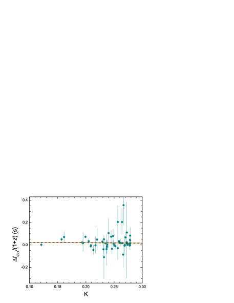
Figure 1.— Dependence of the re-scaled spectral time lag $\Delta t_{\rm obs}/(1+z)$ on the variable $K(z)$. The solid (dashed) line corresponds to the best-fit from the MLE (reduced $\chi^{2}$) method.

4. Results

4.1. Test of the LIV effect

Using the MLE method, we get the resulting constraints on $a_{\rm LIV}$, $\langle b\rangle$, and $\sigma_{\rm int}$, which are displayed in Figure 2(a). These contours show that at the $1\sigma$ confidence level, the best-fit parameters are $a_{\rm LIV}=-0.030^{+0.128}_{-0.127}$ and $\langle b\rangle=0.026^{+0.032}_{-0.032}$, with an intrinsic scatter $\sigma_{\rm int}=0.022^{+0.005}_{-0.005}$. Note that the best-fit value of $a_{\rm LIV}$ is significantly less than its $1\sigma$ uncertainty bounds. This could merely be a statistical fluke that results from the fact that the spectral lag data are quite scattered. The best-fit $\Delta t_{\rm obs}/(1+z)$ versus $K(z)$ function (solid line; with $a_{\rm LIV}=-0.030$ and $\langle b\rangle=0.026$) is plotted in Figure 1, together with the data from GRBs. We also use the reduced $\chi^{2}$ method to constrain the coefficients $a_{\rm LIV}$ and $\langle b\rangle$. This method also takes into account the effect of intrinsic scatter, i.e.,

$$\chi^{2}=\sum_{i}\frac{\left(\frac{\Delta t_{i}}{1+z_{i}}-a_{\rm LIV}K_{i}-\langle b\rangle\right)^{2}}{\sigma_{\rm int}^{2}+\left(\frac{\sigma_{\Delta t_{i}}}{1+z_{i}}\right)^{2}}\;,$$ (9)

where the intrinsic scatter $\sigma_{\rm int}$ is set by requiring that the reduced $\chi^{2}$ equal unity, which is widely used in Type Ia supernova cosmology (e.g., Suzuki et al. 2012). Here the value of $\sigma_{\rm int}$ is 0.021 when the reduced $\chi^{2}$ is unity. We show the constraints from the reduced $\chi^{2}$ method in Figure 2(b). The best-fit values are $a_{\rm LIV}=-0.031^{+0.116}_{-0.116}$ and $\langle b\rangle=0.026^{+0.029}_{-0.029}$, which are quite consistent with those determined from the MLE method. The corresponding best-fit $\Delta t_{\rm obs}/(1+z)$ versus $K(z)$ function is presented in Figure 1 with a dashed line.

Since $a_{\rm LIV}=\Delta E^{\prime}/H_{0}E_{\rm QG}$, for a given $\Delta E^{\prime}$, $a_{\rm LIV}\rightarrow 0$ gives $E_{\rm QG}\rightarrow\infty$. Our constraints show that the slope $a_{\rm LIV}$ is consistent with $0$ within the $1\sigma$ confidence level, and therefore there is no evidence of LIV. That is, Lorentz invariance is consistent with the data.

Marginalizing the likelihood function over the intercept parameter $\langle b\rangle$ and the intrinsic scatter $\sigma_{\rm int}$, one can place 95% confidence limit on the energy scale $E_{\rm QG}$ of LIV by solving the equation (Ellis et al., 2006)

$$\frac{\int_{E_{\rm QG}}^{E_{\infty}}\mathcal{L}_{\rm marg}(E)\;{\rm d}E}{\int_{0}^{E_{\infty}}\mathcal{L}_{\rm marg}(E)\;{\rm d}E}=\frac{\int_{a_{\rm min}}^{a_{\rm LIV}}\mathcal{L}_{\rm marg}(a)\;{\rm d}a}{\int_{a_{\rm min}}^{\infty}\mathcal{L}_{\rm marg}(a)\;{\rm d}a}=0.95\;,$$ (10)

where $E_{\infty}$ represents a reference point fixing the normalization. Here we choose the Planck energy scale as the reference point $E_{\infty}=10^{19}$ GeV, and then $a_{\rm min}=\Delta E^{\prime}/H_{0}E_{\infty}$. Also, $\Delta E^{\prime}=E^{\prime}_{h}-E^{\prime}_{l}$ is the energy difference between the fixed rest-frame energy bands. The 95% confidence-level lower limit obtained by solving Equation (10) is

$$E_{\rm QG}\geq 2.0\times 10^{14}\;{\rm GeV}$$ (11)

for the MLE method, and

$$E_{\rm QG}\geq 2.2\times 10^{14}\;{\rm GeV}$$ (12)

for the reduced $\chi^{2}$ method.

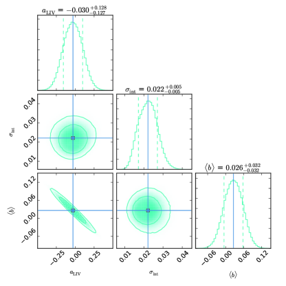
(a)  The maximum likelihood estimation method

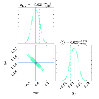
(b)  The reduced $\chi^{2}$ method

Figure 2.— (a): 1D marginalized distributions and 2D regions with the $1\sigma$ and $2\sigma$ contours of the LIV parameters. The vertical solid lines represent the best-fits, and the vertical dashed lines enclose the 68% credible region. Made with triangle.py from Foreman-Mackey et al. (2013). The fitting method employed is MLE. (b): Same as panel (a), but now with the reduced $\chi^{2}$ method.

4.2. Test redshift variation of the LIV effect

To test whether the LIV effect varies with redshift, we divide the sample of 56 GRBs into four groups with redshifts from low to high, each group containing 14 GRBs:

• (A) $0.35\leq z<0.97$, $\langle z\rangle=0.67$;

• (B) $0.97\leq z<1.61$, $\langle z\rangle=1.31$;

• (C) $1.61\leq z\leq 2.20$, $\langle z\rangle=1.93$;

• (D) $2.30\leq z\leq 5.47$, $\langle z\rangle=3.00$.

For each group, we perform the same fit procedure (the MLE method) as applied to the whole GRB sample to optimize the parameters $a_{\rm LIV}$, $\langle b\rangle$ and the intrinsic scatter $\sigma_{\rm int}$, and calculate the mean redshift $\langle z\rangle$. The constraints on the slopes $a_{\rm LIV}$ against $\langle z\rangle$ for four groups are shown in Figure 3, together with the $1\sigma$ error bars of $a_{\rm LIV}$. Since the data points in the second redshift bin are too much scattered, the error bars of $a_{\rm LIV}$ are larger than those of the other three redshift bins. A linear fit to $a_{\rm LIV}$–$\langle z\rangle$ (the solid line in Figure 3) leads to $a_{\rm LIV}=(0.501\pm 0.504)-(0.213\pm 0.261)\langle z\rangle$. Clearly, the slope of $a_{\rm LIV}$ versus $\langle z\rangle$ is consistent with zero at the $1\sigma$ confidence level. This result shows no statistically significant evidence for the redshift evolution of the LIV effect. Moreover, because $a_{\rm LIV}$ is consistent with $a_{\rm LIV}=0$ within the $1\sigma$ confidence level for all four redshift bins, we can conclude that there is no evidence of LIV and results that all are consistent with each other.

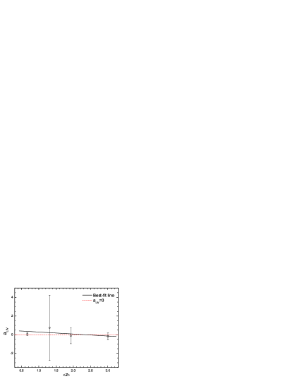
Figure 3.— The fitted values of $a_{\rm LIV}$ against the mean redshift of GRBs. Each data point with $1\sigma$ error bars corresponds to a group of GRBs (A, B, C and D, from left to right). The solid and dashed lines represent the best-fit line and $a_{\rm LIV}=0$, respectively.

5. Discussion and conclusion

The spectral lags of GRBs between two fixed energy bands in the rest frame have been investigated by projecting these two bands to the observer frame. In this work, we first use the rest-frame spectral lags of 56 GRBs to test the possible LIV effect and its redshift dependence. This is a step forward in the investigation of LIV, since all current studies used lags extracted in the observer frame only and the evolution of the LIV effect with redshift has not yet been explored.

The key challenge in such time-of-flight tests, however, is distinguishing an intrinsic time delay at the source from a possible time delay induced by the LIV effect. In order to overcome the intrinsic time delay problem, we perform a linear fit to the spectral lags ($\Delta t_{\rm obs}$, between two fixed rest-frame energy bands in a complete sample of 56 GRBs) versus the $K(z)$ data (it is a function of the redshift), where the slope $a_{\rm LIV}$ in the linear regression analysis corresponds to the QG scale related to the LIV effect, and the intercept $\langle b\rangle$ represents the average effect of the intrinsic time lags of different pulses internal to the GRB. This technique we used was originally proposed by Ellis et al. (2006), while they focused on the observer-frame spectral lags.

With the whole sample, we first optimize the coefficients $a_{\rm LIV}$, $\langle b\rangle$ and the intrinsic scatter $\sigma_{\rm int}$ by maximizing the likelihood function (i.e, the MLE method). The marginalized $1\sigma$ results are $a_{\rm LIV}=-0.030^{+0.128}_{-0.127}$, $\langle b\rangle=0.026^{+0.032}_{-0.032}$, and $\sigma_{\rm int}=0.022^{+0.005}_{-0.005}$. Using the reduced $\chi^{2}$ method, we obtain $a_{\rm LIV}=-0.031^{+0.116}_{-0.116}$ and $\langle b\rangle=0.026^{+0.029}_{-0.029}$. The results from these two fitting methods are in good agreement. Since the slope $a_{\rm LIV}$ is in good agreement with $0$ within the $1\sigma$ confidence level, there is no evidence of LIV. That is, Lorentz invariance is consistent with the data. By marginalizing the likelihood function over $\langle b\rangle$ and $\sigma_{\rm int}$, we obtain the 95% confidence-level lower limit on the energy scale $E_{\rm QG}$ of LIV, yielding $E_{\rm QG}\geq 0.2\times 10^{15}$ GeV. While our constraint is not the tightest, there is nonetheless merit to the result. Thanks to our improved statistical technique and the first use of the rest-frame spectral lags, our constraint is much more statistically significant than previous results.

By dividing the 56 GRBs into four groups according to their redshifts and fitting each group separately, we find the best-fit values of $a_{\rm LIV}$ do not vary with the cosmological redshift, implying there is no evidence for the reshift evolution of the LIV effect. Moreover, because $a_{\rm LIV}$ is consistent with $a_{\rm LIV}=0$ within the $1\sigma$ confidence level for all four redshift bins, we can conclude that Lorentz invariance is consistent with the data for all four redshift bins. This is the first time to explore the redshift variation of the LIV effect.

References

- Abdo et al. (2009a) Abdo, A. A., Ackermann, M., Ajello, M., et al. 2009a, Nature, 462, 331
- Abdo et al. (2009b) Abdo, A. A., Ackermann, M., Arimoto, M., et al. 2009b, Science, 323, 1688
- Amelino-Camelia (2013) Amelino-Camelia, G. 2013, Living Reviews in Relativity, 16, 5
- Amelino-Camelia et al. (2017a) Amelino-Camelia, G., D’Amico, G., Rosati, G., & Loret, N. 2017a, Nature Astronomy, 1, 0139
- Amelino-Camelia et al. (2017b) Amelino-Camelia, G., D’Amico, G., Fiore, F., Puccetti, S., & Ronco, M. 2017b, ArXiv e-prints, arXiv:1707.02413
- Amelino-Camelia et al. (1997) Amelino-Camelia, G., Ellis, J., Mavromatos, N. E., & Nanopoulos, D. V. 1997, International Journal of Modern Physics A, 12, 607
- Amelino-Camelia et al. (1998) Amelino-Camelia, G., Ellis, J., Mavromatos, N. E., Nanopoulos, D. V., & Sarkar, S. 1998, Nature, 393, 763
- Amelino-Camelia & Piran (2001) Amelino-Camelia, G., & Piran, T. 2001, Phys. Rev. D, 64, 036005
- Amelino-Camelia & Smolin (2009) Amelino-Camelia, G., & Smolin, L. 2009, Phys. Rev. D, 80, 084017
- Bernardini et al. (2015) Bernardini, M. G., Ghirlanda, G., Campana, S., et al. 2015, MNRAS, 446, 1129
- Biesiada & Piórkowska (2009) Biesiada, M., & Piórkowska, A. 2009, Classical and Quantum Gravity, 26, 125007
- Bluhm (2005) Bluhm, R. 2005, ArXiv High Energy Physics - Phenomenology e-prints, hep-ph/0506054
- Boggs et al. (2004) Boggs, S. E., Wunderer, C. B., Hurley, K., & Coburn, W. 2004, ApJ, 611, L77
- Chang et al. (2012) Chang, Z., Jiang, Y., & Lin, H.-N. 2012, Astroparticle Physics, 36, 47
- Coleman & Glashow (1999) Coleman, S., & Glashow, S. L. 1999, Phys. Rev. D, 59, 116008
- D’Agostini (2005) D’Agostini, G. 2005, ArXiv Physics e-prints, physics/0511182
- Ellis et al. (2000) Ellis, J., Farakos, K., Mavromatos, N. E., Mitsou, V. A., & Nanopoulos, D. V. 2000, ApJ, 535, 139
- Ellis & Mavromatos (2013) Ellis, J., & Mavromatos, N. E. 2013, Astroparticle Physics, 43, 50
- Ellis et al. (2008) Ellis, J., Mavromatos, N. E., & Nanopoulos, D. V. 2008, Physics Letters B, 665, 412
- Ellis et al. (2011) —. 2011, International Journal of Modern Physics A, 26, 2243
- Ellis et al. (2003) Ellis, J., Mavromatos, N. E., Nanopoulos, D. V., & Sakharov, A. S. 2003, A&A, 402, 409
- Ellis et al. (2006) Ellis, J., Mavromatos, N. E., Nanopoulos, D. V., Sakharov, A. S., & Sarkisyan, E. K. G. 2006, Astroparticle Physics, 25, 402
- Foreman-Mackey et al. (2013) Foreman-Mackey, D., Hogg, D. W., Lang, D., & Goodman, J. 2013, PASP, 125, 306
- Hakkila & Giblin (2004) Hakkila, J., & Giblin, T. W. 2004, ApJ, 610, 361
- Hakkila & Nemiroff (2009) Hakkila, J., & Nemiroff, R. J. 2009, ApJ, 705, 372
- Jacob & Piran (2007) Jacob, U., & Piran, T. 2007, Nature Physics, 3, 87
- Jacob & Piran (2008) —. 2008, JCAP, 1, 031
- Kahniashvili et al. (2006) Kahniashvili, T., Gogoberidze, G., & Ratra, B. 2006, Physics Letters B, 643, 81
- Kocevski & Liang (2003) Kocevski, D., & Liang, E. 2003, ApJ, 594, 385
- Kostelecký & Mewes (2008) Kostelecký, V. A., & Mewes, M. 2008, ApJ, 689, L1
- Kostelecký & Mewes (2013) —. 2013, Physical Review Letters, 110, 201601
- Kostelecký & Potting (1991) Kostelecký, V. A., & Potting, R. 1991, Nuclear Physics B, 359, 545
- Kostelecký & Potting (1995) —. 1995, Phys. Rev. D, 51, 3923
- Kostelecký & Russell (2011) Kostelecký, V. A., & Russell, N. 2011, Reviews of Modern Physics, 83, 11
- Kostelecký & Samuel (1989) Kostelecký, V. A., & Samuel, S. 1989, Phys. Rev. D, 39, 683
- Liberati (2013) Liberati, S. 2013, Classical and Quantum Gravity, 30, 133001
- Mattingly (2005) Mattingly, D. 2005, Living Reviews in Relativity, 8, 5
- Nemiroff (2000) Nemiroff, R. J. 2000, ApJ, 544, 805
- Nemiroff (2012) —. 2012, MNRAS, 419, 1650
- Nemiroff et al. (2012) Nemiroff, R. J., Connolly, R., Holmes, J., & Kostinski, A. B. 2012, Physical Review Letters, 108, 231103
- Norris (2002) Norris, J. P. 2002, ApJ, 579, 386
- Norris et al. (2005) Norris, J. P., Bonnell, J. T., Kazanas, D., et al. 2005, ApJ, 627, 324
- Pan et al. (2015) Pan, Y., Gong, Y., Cao, S., Gao, H., & Zhu, Z.-H. 2015, ApJ, 808, 78
- Pavlopoulos (1967) Pavlopoulos, T. G. 1967, Physical Review, 159, 1106
- Pavlopoulos (2005) —. 2005, Physics Letters B, 625, 13
- Planck Collaboration et al. (2016) Planck Collaboration, Ade, P. A. R., Aghanim, N., et al. 2016, A&A, 594, A13
- Schaefer (1999) Schaefer, B. E. 1999, Physical Review Letters, 82, 4964
- Shao et al. (2010) Shao, L., Xiao, Z., & Ma, B.-Q. 2010, Astroparticle Physics, 33, 312
- Suzuki et al. (2012) Suzuki, N., Rubin, D., Lidman, C., et al. 2012, ApJ, 746, 85
- Tasson (2014) Tasson, J. D. 2014, Reports on Progress in Physics, 77, 062901
- Ukwatta et al. (2012) Ukwatta, T. N., Dhuga, K. S., Stamatikos, M., et al. 2012, MNRAS, 419, 614
- Vasileiou et al. (2013) Vasileiou, V., Jacholkowska, A., Piron, F., et al. 2013, Phys. Rev. D, 87, 122001
- Wei et al. (2016) Wei, J.-J., Wu, X.-F., Gao, H., & Mészáros, P. 2016, JCAP, 8, 031
- Wei et al. (2013) Wei, J.-J., Wu, X.-F., & Melia, F. 2013, ApJ, 772, 43
- Wei et al. (2015) Wei, J.-J., Wu, X.-F., Melia, F., & Maier, R. S. 2015, AJ, 149, 102
- Wei et al. (2017a) Wei, J.-J., Zhang, B.-B., Shao, L., Wu, X.-F., & Mészáros, P. 2017a, ApJ, 834, L13
- Wei et al. (2017b) Wei, J.-J., Wu, X.-F., Zhang, B.-B., et al. 2017b, ApJ, 842, 115
- Xiao & Ma (2009) Xiao, Z., & Ma, B.-Q. 2009, Phys. Rev. D, 80, 116005
- Xu & Ma (2016) Xu, H., & Ma, B.-Q. 2016, Astroparticle Physics, 82, 72
- Zhang (2012) Zhang, F.-W. 2012, Ap&SS, 339, 123
- Zhang & Ma (2015) Zhang, S., & Ma, B.-Q. 2015, Astroparticle Physics, 61, 108