SYGMA: Stellar Yields for Galactic Modeling Applications

Abstract

The Stellar Yields for Galactic Modeling Applications (SYGMA) code is an open-source module that models the chemical ejecta and feedback of simple stellar populations (SSPs). It is intended for use in hydrodynamical simulations and semi-analytic models of galactic chemical evolution. The module includes the enrichment from asymptotic giant branch (AGB) stars, massive stars, Type-Ia supernovae (SNe Ia) and compact binary mergers. An extensive and extendable stellar yields library includes the NuGrid yields with all elements and many isotopes up to Bi. Stellar feedback from mechanic and frequency-dependent radiative luminosities are computed based on NuGrid stellar models and their synthetic spectra. The module further allows for customizable initial-mass functions and SN Ia delay-time distributions to calculate time-dependent ejecta based on stellar yield input. A variety of r-process sites can be included. A comparison of SSP ejecta based on NuGrid yields with those from Portinari et al. (1998) and Marigo (2001) reveals up to a factor of 3.5 and 4.8 less C and N enrichment from AGB stars at low metallicity, a result we attribute to NuGrid’s modeling of hot-bottom burning. Different core-collapse supernova explosion and fallback prescriptions may lead to substantial variations for the accumulated ejecta of C, O and Si in the first $10^{7}\,\mathrm{yr}$ at $Z=0.001$. An online interface of the open-source SYGMA module enables interactive simulations, analysis and data extraction of the evolution of all species formed by the evolution of simple stellar populations.

1 Introduction

Galactic chemical evolution (GCE) models (see, e.g., Audouze & Tinsley, 1976; Arnett, 1996) require as input the time-dependent nucleosynthetic output returned to the interstellar medium by evolving stars and stellar explosions. These metallicity-dependent yields are combined to represent a simple stellar population (SSP), and includes material processed by low-mass stars, massive star winds, supernovae, and merger events. SSPs are the core building blocks of galactic chemical evolution models, and are used as input in hydrodynamic cosmological structure and galaxy formation simulations (e.g.  Wiersma et al., 2009; Few et al., 2014; Somerville & Davé, 2015).

In this paper, we present the open-source, time-dependent SSP module Stellar Yields for Galactic Modeling Applications (SYGMA). It implements easily-modifiable prescriptions for the initial mass function (IMF), stellar lifetimes, wind mass-loss histories and merger timescales. It can also be used in a stand-alone manner to assess the impact of stellar evolution and nucleosynthesis modeling assumptions. The concept of an SSP module is not new, and several alternative SSP codes can be found in the literature (e.g., Gibson 1995, 1997; Leitherer et al. 1999; Kawata & Gibson 2003; Few et al. 2012, 2014; Rybizki et al. 2017; Saitoh 2017).

SYGMA is part of the open-source python chemical evolution NuGrid framework NuPyCEE, includes examples and analysis tools, and represents the fundamental building-block component of our JINA-NuGrid chemical evolution pipeline (Côté et al. 2017b). This pipeline creates an integrated workflow that links basic stellar and nuclear physics investigations of the formation of elements in stars and stellar explosions, to SSPs, GCE and semi-analytic models (Côté et al. 2018), and ultimately hydrodynamic cosmological simulations.

SYGMA includes a number of published yield sets available as options in NuPyCEE which can be used to compare SYGMA SSP models with those using the latest set of NuGrid yields (Pignatari et al., 2016; Ritter et al., 2017). The NuGrid yields have been derived from low-mass and massive star evolution and nucleosynthesis simulations created with the same codes for the entire mass range. All models adopt – as much as possible – the same physics assumptions, including macro physics and nuclear reaction rates, for the entire mass range. This makes the NuGrid yield set the most internally consistent data set presently available.

The impact of yield uncertainties on GCE predictions has been shown in Gibson (2002) and Romano et al. (2010). Wiersma et al. (2009, W09) developed a chemical feedback module for hydrodynamic simulations, and found that their SSP ejecta can differ by a factor of two or more for different yields available in literature.

Aside from enriching the ISM, stars also alter the surrounding medium through winds and radiation. These energy inputs into the ISM are the basis of the stellar ‘feedback’ introduced in most galaxy simulation codes. A common approach is to adopt feedback prescriptions that neglect their dependence on the stellar models from which the yields are derived. W09, for example, adopt a constant kinetic energy of $10^{51}\,\mathrm{erg}$ for stars above the zero-age main-sequence mass of $M_{\rm ZAMS}=6\,M_{\odot}$. SYGMA implements these energy sources based on the stellar models and supernova explosions from the same NuGrid data set from which the yields were derived.

We present the functionality of our code in Sect. 2. In Sect. 3 we analyze the ejecta of SSPs at solar metallicity and low metallicity based on the new NuGrid yields (Pignatari et al., 2016; Ritter et al., 2017) compared to the combined yield set of AGB yields of Marigo (2001a, M01) and massive star yields of Portinari et al. (1998, P98). Also discussed are the effects of core-collapse mass-cut prescriptions on yields from massive star models. In Sect. 4 we summarize our results. An appendix provides information on code verification and online access.

2 Methods

SYGMA is part of NuPyCEE which, together with the yield data used in this paper, is available on GitHub. For this work, we use NuPyCEE version 3.0, which can be recovered via Zenodo (Ritter et al. 2018).

2.1 Simple Stellar Population Mechanics

A simple stellar population consists of an ensemble of stars of common age and metallicity. Chemical evolution assumptions describe properties of the stellar population such as the number of stars formed in a initial mass range. Results shown in this section are based on NuGrid yields (Ritter et al., 2017), Type Ia supernovae (SNe Ia) yields from Thielemann et al. (1986) and NS merger yields from Rosswog et al. (2014).

2.1.1 Simple Stellar Population Ejecta

The cumulative contributions from AGB stars, massive stars and SNe Ia are tracked separately (Figure 1). SYGMA provides analytic tools to identify the most relevant nuclear production site for a given element or isotope. For example, in an SSP at $Z=0.02$, AGB stars (Figure 1) produce about 64% of the total amount of C (e.g. Schneider et al., 2014), while massive stars produce 62% of the total amount of O (e.g. Woosley et al., 2002). SNe Ia produce 63% of Fe (e.g. Thielemann et al., 1986). All stable elements and most isotopes up to Bi are tracked (Figure 1). To model the element enrichment through other sources such as r-process from neutrino-driven winds additional yields can be included as extra yield tables.

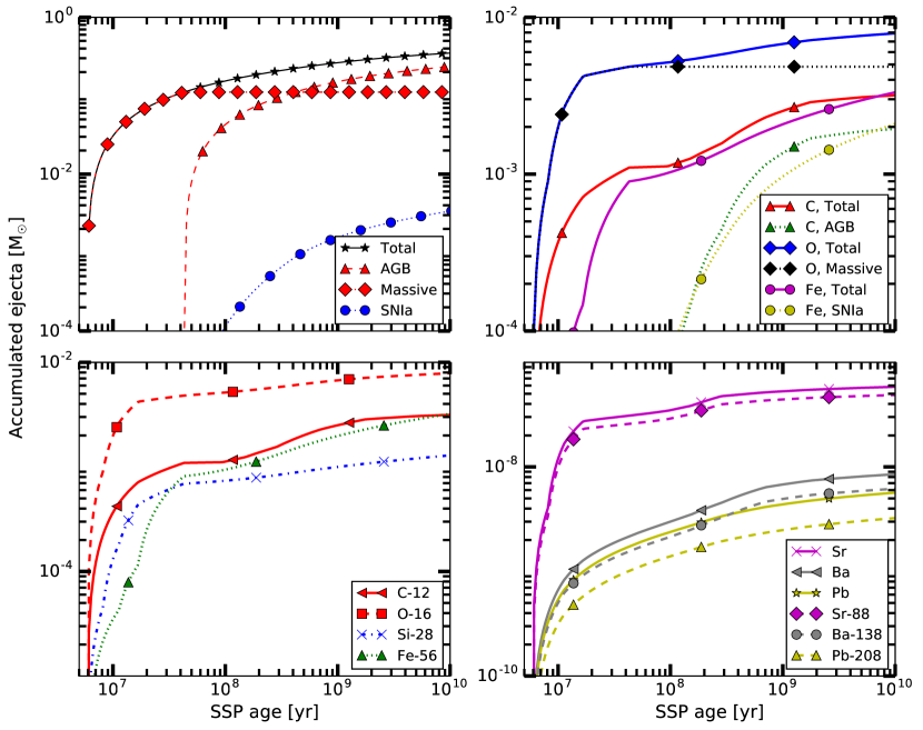
Figure 1: Accumulated ejecta from AGB stars, massive stars and SNe Ia for a SSP at $Z=0.02$ (top, left). The mass of the SSP is set to 1$\,M_{\odot}$ so that the SSP ejecta represents the mass ejected per units of stellar mass formed. Accumulated ejecta of C, O and Fe from all (total) or from distinct sources (top, right). Ejecta from of abundant isotopes of C, O, Si and Fe (bottom, left). Total accumulated ejecta of isotopes and elements of intermediate mass and from the first, second and third s-process peak (bottom, right). Access and interactive exploration of the figures is possible with the WENDI interface (Appendix B).

SYGMA adopts the delayed production approximation (Pagel, 2009). The stellar lifetimes are based on the same stellar evolution models as the yields. For AGB models they are the stellar lifetimes until the end of the computation during the thermal-pulse AGB stage or until the end of the post-AGB stage. For massive star models the time span is the time until core collapse. The time span or lifetime $\tau$ is interpolated using a log-log spline fit of the tabulated lifetimes and initial masses.

The mass $\Delta\mathrm{M}_{\rm SSP}$ lost by a SSP over the time interval [$t$,$t$+$\Delta t$] is

$$\Delta\mathrm{M}_{\rm SSP}=\int_{t}^{t+\Delta t}\xi(M_{\tau}(t^{\prime}))\,M_{\star}(M_{\tau}(t^{\prime}),Z)\,dt^{\prime}$$ (1)

where $M_{\tau}(t)$ is the inverse of the lifetime function $\tau(M)$. $\xi(M)$ is the IMF normalized to the total stellar mass of the SSP and $M_{\star}(M,Z)$ is the total ejected mass of the stars of mass $M$ and metallicity $Z$.

2.1.2 Initial Mass Function

The IMF $\xi$ gives the number of stars $N$ within an initial mass interval [$m_{1}$,$m_{2}$] via

$$N=A\int_{m_{1}}^{m_{2}}{\xi(m^{\prime})}\,dm^{\prime}$$ (2)

where the normalization constant $A$ is derived from the total stellar mass. SYGMA provides a number of options (see Kroupa et al., 2013, for discussion), such as the Salpeter IMF (Salpeter 1955)

$$\xi(m)=A_{S}\,m^{-\alpha}$$ (3)

where $\alpha=2.35$ ($\alpha$ can be changed as input parameter), and the Chabrier IMF (Chabrier 2003)

$${}\xi(m)={}$$

(4)

where $m_{c}=0.079$ and $\sigma=0.69$. The Kroupa IMF (Kroupa 2001)

$${}\xi(m)={}$$

(5)

is provided as well. A custom IMF can be defined as well in the code and in the online version. The lower and upper boundaries of the IMF are input parameters, and related to the onset of H-burning and the occurrence of the most massive stars respectively (see discussion in Côté et al., 2016).

2.1.3 Type Ia Supernova Rates

The number of SNe Ia $N_{\rm Ia}$ per unit of $\,M_{\odot}$ formed in the time interval [$t$,$t$+$\Delta t$] is given by

$$N_{\rm Ia}=A_{\rm Ia}\int_{t}^{t+\Delta t}f_{WD}(t^{\prime})\ \Psi_{\rm Ia}(t^{\prime})\,dt^{\prime}$$ (6)

where $A_{\rm Ia}$ is a normalization constant, $f_{\rm WD}(t)$ is the fraction of white dwarfs and $\Psi_{\rm Ia}(t)$ is the delay-time distribution (DTD) at time $t$ (W09). White dwarfs with initial masses between $3\,M_{\odot}$ and $8\,M_{\odot}$ are potential SN Ia progenitors, as commonly adopted (e.g. Dahlen et al., 2004; Mannucci et al., 2006, W09). Either $A_{\rm Ia}$ or the total number of SNe Ia per $\,M_{\odot}$ are required as an input. The power-law DTD of Maoz & Mannucci (2012)

$$\Psi_{\rm Ia}(t)=t^{-1}$$ (7)

can be selected, and the power-law exponent can be an input parameter. An exponential DTD in the form of

$$\Psi_{\rm Ia}(t)=\frac{e^{-t/\tau_{\rm Ia}}}{\tau_{\rm Ia}}$$ (8)

and a Gaussian DTD as

$$\Psi_{\rm Ia}(t)=\frac{1}{\sqrt{2\pi\sigma^{2}}}e^{-\frac{(t-\tau_{\rm Ia})^{2}}{2\sigma^{2}}}$$ (9)

are other options, as in W09. $\tau_{\rm Ia}$ is the characteristic delay time and $\sigma$ defines the width of the Gaussian distribution. For a discussion of the parameters see W09 and references within. More generally, arbitrary delay-time distribution functions may be used with the delayed-extra source option to explore new scenarios or to account for the individual contribution of different SN Ia channels.

2.1.4 Neutron Star Merger Rates

The number of NS mergers $N_{\rm NS}$ in the time interval [$t$,$t$+$\Delta t$] is given as

$$N_{\rm NS}=A_{\rm NS}\int_{t}^{t+\Delta t}\Psi_{\rm NS}(t^{\prime},Z)\,dt^{\prime}$$ (10)

where $A_{\rm NS}$ is a normalization constant and $\Psi_{\rm NS}(t,Z)$ is the NS DTD. The user can choose between a power law DTD, the DTD of Dominik et al. (2012), or a constant coalescence time. For the DTD based on Dominik et al. (2012) we adopt for the metallicity of $Z\geq 0.019$ their DTD at solar metallicity and for $Z\leq 0.002$ their DTD at a tenth of solar metallicity. We interpolate the distribution between these two metallicity boundaries. The normalization constant $A_{\rm NS}$ is derived from the total number of merger systems $N_{\rm NS,tot}$ via

$$A_{\rm NS}=\frac{N_{\rm NS,tot}}{\int_{0}^{\infty}\Psi_{\rm NS}(t,Z)\,dt^{\prime}}.$$ (11)

$N_{\rm NS,tot}$ is calculated as

$$N_{\rm NS,tot}=0.5\,f_{m}\,f_{b}\int_{m_{1}}^{m_{2}}\xi(m^{\prime})\,dm^{\prime}$$ (12)

where $f_{m}$ is the fraction of merger of massive-star binary systems and $f_{b}$ is the binary fraction of all massive stars. $f_{m}$ and $f_{b}$ as well as the initial mass range for potential merger progenitors [$m_{1}$,$m_{2}$] need to be provided as an input. For normalizing the number of NS merger with Eq. (10), the user can also directly normalize the rate by providing the total number of NS merger per unit of $\,M_{\odot}$ formed as an input.

With SYGMA, the DTD of NS mergers can also be defined by a simple power law. In that case, the power-law index and the minimum and maximum coalescence timescales must be provided as input parameters. Alternatively, arbitrary DTD functions can be assigned to NS mergers using our delayed-extra source implementation. This option can also be used for black hole neutron star mergers and for different SN Ia channels.

2.1.5 Yield Implementation

The total yields $y_{\mathrm{tot},i}$ are defined as the total mass of element/isotope $i$ ejected over the lifetime of the star and given as

$$y_{\mathrm{tot},i}=y_{0,i}+y_{n,i}$$ (13)

where $y_{0,i}$ refers to the mass of element/isotope $i$ initially available in the stellar simulation. The net yields $y_{n,i}$ is the produced or destroyed mass of element/isotope $i$. Yield tables with total yields are the default input for SYGMA.

With the application of total yields the assumption holds that the initial abundance of the underlying stellar model $y_{0,i}$ represents the gas composition of the chemical evolution simulation $y_{0,\mathrm{sim},i}$ at the time of star formation. If material is unprocessed throughout stellar evolution the total ejecta is $y_{\mathrm{tot},i}=y_{0,i}$ and the error $\epsilon_{i}=y_{0,\mathrm{sim},i}-y_{0,i}$ propagates into the total ejecta. This could lead with $\epsilon_{j}>0$ to the artificial production of isotope $j$ (for example in the case of r-process species) if it is based solely on the solar-scaled initial abundance. For element/isotope $k$ of secondary nucleosynthesis origin $y_{n,k}$ depends strongly on $y_{0,k}$ and on the error $|\epsilon_{k}|$.

Net yields can be applied in the code to take into account $y_{0,\mathrm{sim},i}$ and SYGMA calculates the total ejecta $y_{\mathrm{tot},i}$ as

$$y_{tot,i}=y_{0,sim,i}+y_{n,i}.$$ (14)

With the destruction of element/isotope $h$ ($y_{n,h}<0$) and $\epsilon_{h}<0$ more of element/isotope $h$ is destroyed than initially available and the error is $|\epsilon_{h}|$. In this case the code sets $y_{\mathrm{tot},h}=0$. For SN Ia only total yields can be used.

An initial mass interval can be specified to take into account material locked away in massive stars through black hole formation. This IMF yield range goes by default from $M_{\rm ZAMS}=1\,M_{\odot}$ to $M_{\rm ZAMS}=30\,M_{\odot}$. The IMF yield range and the IMF range can both be set separately for stars of $Z>0$ and Pop III stars to take into account different types of star formation.

The yields of a specific tabulated stellar model are applied to all stars included in a certain interval of initial stellar masses. The lower and upper boundaries of this interval represent half the distance to the next available lower- and higher-mass tabulated stellar model, respectively. For a given initial mass in this interval, the yields of the selected tabulated stellar model are re-normalized according to the fitted relation between the initial stellar mass and the total ejected mass.

2.1.6 Stellar Feedback

Mass-loss rates from stellar winds, stellar luminosities of different energy bands, and kinetic energies of SN of SSPs can be modeled with additional input tables.

Stellar winds

The properties of stellar winds are of importance since these winds can contribute to galactic winds which distribute metals and enrich the intergalactic medium (Hopkins et al., 2012). We provide the time evolution of the mass ejection rates of AGB and massive star models as an input for SYGMA. The mass-loss rates of SSPs decrease with time due to the declining AGB mass loss rates towards lower initial masses. The mass-loss rates shown in Figure 2 for a SSP of $1\,M_{\odot}$ at solar metallicity are similar to Figures 3 and 4 in Côté et al. (2015). Throughout this paper, we choose $1\,M_{\odot}$ for the mass of our SSPs so that the stellar ejecta represents the normalized mass ejected per units of stellar mass formed. When comparing with Côté et al. (2015), which adopted SSPs of $10^{6}\,M_{\odot}$, our results need to be scaled up by a factor of $10^{6}$.

The steps in the evolution of the ejected mass originate from the transition between grid points of the stellar model grid. The strongest AGB mass loss originates from the $5\,M_{\odot}$ stellar model, as visible in the peak shortly after $10^{8}\,\mathrm{yr}$. To determine the kinetic energy of stellar winds $\,E_{\rm wind}$ we calculate for each stellar model the time-dependent escape velocity $v_{\rm esc}$.

After deriving the terminal velocity $v_{\infty}$ from $v_{\rm esc}$ one can calculate the kinetic energy as

$$\,E_{\rm wind}(t)=\frac{1}{2}\dot{m}(t)v_{\infty}(t)^{2}.$$ (15)

Abbott (1978) found the relation $v_{\infty}=3v_{\rm esc}$ for observed O, B, A and Wolf-Rayet stars via radiation-driven wind theory. We apply this relation because $\,E_{\rm wind}$ originates mainly from the most massive stars with radiative winds (Leitherer et al., 1992).

The stellar grid includes stellar models up to $M_{\rm ZAMS}=25\,M_{\odot}$, while stellar models at higher initial mass are expected to contribute the majority of the kinetic wind energy of the stellar population. Hence our kinetic energy of winds are similar to those of the SSP with upper IMF limit of $30\,M_{\odot}$ of starburst99 (Fig. 111, Leitherer et al., 1999).

For AGB models we approximate $v_{\infty}$ as $v_{\infty}=v_{\rm esc}$ which might overestimate the kinetic energy contribution of the AGB phase as indicated by observations (Bolton, 2000). Energetic contributions of AGB stars are often not considered in SSP models since their contribution is negligible compared to massive stars (Leitherer et al., 1999; Côté et al., 2015). Our largest kinetic energies of winds originate from massive star models while the kinetic energies of winds from AGB models are considerably smaller (Figure 2).

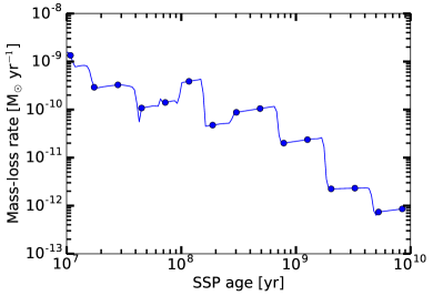
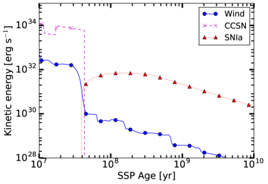
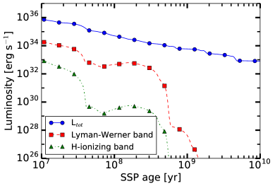
Figure 2: Evolution of mass ejection of a SSP of $1\,M_{\odot}$ at $Z=0.02$ (top). Kinetic energies of stellar winds, CC SNe and SNe Ia (middle). Time dependence of the total luminosity and luminosities in the Lyman-Werner and H-ionizing bands emitted by the SSP (bottom).

Table 1: Properties of yield sets of AGB and massive stars available in SYGMA. Shown are the NuGrid sets (Pignatari et al., 2016; Ritter et al., 2017) as well as low mass /massive star yield combinations M01P98 (Marigo, 2001b; Portinari et al., 1998), K10K06 (Kobayashi et al., 2006; Karakas et al., 2010) and C15K06 (Cristallo et al., 2015; Kobayashi et al., 2006). Properties are the initial mass and metallicity range, available S-AGB models, the modeled heavy-element processes, the heaviest available stable element in the network provided and the modeling of the CCSN explosion.

ID	Masses	Metallicity	S-AGB	Heavy-element processes	Network	Exp
NuGrid	$1-25$	$0.0001-0.02$	yes	main s, weak s, p, $\gamma$	Pb	yes
M01P98	$1-120$	$0.0004-0.05$	no	-	Fe	no
K10K06	$1-40$	$0.0001-0.02$	no	-	Ni	yes
C15K06	$1.3-40$	$0.0001-0.02$	no	main s	Ge	yes

Supernova energies

The kinetic energies of core-collapse supernovae (CCSNe) is usually taken as $10^{51}\,\mathrm{erg}$, which is similar to the observed explosion energies of SN such as SN 1987A (Arnett et al., 1989). We apply CCSN energies based on the CCSN explosion prescription of Fryer et al. (2012) used for NuGrid stellar models. For each initial mass and metallicity of the stellar models the kinetic energy is extracted from Fig. 2 of Fryer et al. (2012). Energies for stellar models above $25\,M_{\odot}$ are not taken into account. Such stellar models are not included in the NuGrid model grid because they do not explode according to our remnant mass model. The kinetic energy of a SNe Ia is an input parameter of SYGMA and is set to $10^{51}\,\mathrm{erg}$.

For a SSP of $1\,M_{\odot}$ at solar metallicity, the kinetic energy from CC SN explosions of $\approx 10^{34}\,\mathrm{erg\,s}^{-1}$ is similar to starburst99 (Fig. 113, Leitherer et al., 1999). The kinetic energies from SNe Ia is more than $1\,\mathrm{dex}$ lower than the kinetic energy from CC SN explosions (Figure 2) and very similar to Côté et al. (2015, Fig. 4). In Leitherer et al. (1999) and Côté et al. (2015), the mass of the SSPs are 10${}^{6}\,M_{\odot}$, so our results need to be scaled up by a factor of 10⁶ when doing the comparison.

Stellar luminosities

Stellar radiation alters the surrounding medium through ionization and radiation pressure. SYGMA computes luminosities of SSPs based on time-dependent bolometric luminosities of stellar models. The latter are provided as table input. The luminosities in specific wavelength bands such as the H-ionizing band ($13.6\,\mathrm{eV}$ - $24.6\,\mathrm{eV}$) are calculated as well as the time-dependent luminosities of luminosity bands based on spectra of the stellar evolution models. The latter are from the PHOENIX (Husser et al., 2013) and ATLAS9 (Castelli & Kurucz, 2004) synthetic spectra libraries.

Spectra are derived from the best match of effective temperature $T_{\rm eff}$, gravity $g$, [Fe/H] and $\alpha$-enhancement of a stellar model. We adopt the $\alpha$-enhancement of the initial abundance of the stellar models and neglect any changes of the surface abundance during stellar evolution. The $\alpha$-enhancement at low metallicity of NuGrid models is based on observations of individual elements and each element has its own enhancement. The corresponding average $\alpha$-enhancement is [$\alpha$/Fe] = 0.8 by taking into account the initial abundance of each element. The total luminosity, as well as the luminosity in two wavelength bands, of an SSP of $1\,M_{\odot}$ at $Z=0.02$ are shown in the lower panel of Figure 2.

2.2 Stellar Yields

Metallicities for which stellar yields are provided can be selected as initial metallicities of the SSP. The number of isotopes included in SYGMA is flexible and is automatically set when reading the input yield tables. The lifetime and final mass for each star are required in the yield input tables. In the following we introduce the yield sets of our comprehensive yield library for SYGMA. Additional yields can be added on request.

The default yields of AGB models, massive star models and core-collapse supernova models are from the NuGrid collaboration and include the metallicities $Z=0.02$, $0.01$, $0.006$, $0.001$, and $0.0001$ (yield sets NuGrid_d/r/m, Table 1, Ritter et al., 2017). Yields for twelve stellar models between $M_{\rm ZAMS}=1\,M_{\odot}$ and $M_{\rm ZAMS}=25\,M_{\odot}$ are provided for each metallicity, including super-AGB models.

To briefly summarize, the thermal pulse AGB (TP-AGB) stages of low- and intermediate-mass stars and all burning stages of massive stars until collapse are included. All stable elements and many isotopes up to Bi are provided in the yield tables. Convective boundary mixing is applied at all convection zones in AGB models. A nested-network approach resolves hot-bottom burning during post-processing and predicts isotopes of the CNO cycle and s process isotopes. As part of the semi-analytic explosion prescription a mass- and metallicity dependent fallback is applied which accounts for the observed NS and BH mass distribution. Fallback in stellar models of high initial mass leads to black hole formation. Yield sets are available for delayed explosions (NuGrid_d), rapid explosions (NuGrid_r) and a combination of both (NuGrid_m, see Sect. 3.3). The NuGrid data is available online as tables and through the WENDI interface (Appendix B).

The yield set of the Padua group (M01P98) consists of AGB yields from M01 and massive star yields from P98. Stellar yields for initial masses between $M_{\rm ZAMS}=1\,M_{\odot}$ and $M_{\rm ZAMS}=120\,M_{\odot}$ and $Z=0.02,0.008,0.004,0.0004$ are available. The AGB stage of stellar models up to $M_{\rm ZAMS}=5\,M_{\odot}$ is based on synthetic models which are calibrated against observations. For stellar mass models with $M_{\rm ZAMS}=6\,M_{\odot}$ and $M_{\rm ZAMS}=7\,M_{\odot}$ the AGB stage is not modeled. The contribution from CCSN nucleosynthesis of the massive star models is derived from the explosions of massive star models of Woosley & Weaver (1995).

AGB yields from Karakas et al. (2010) and massive star yields from Kobayashi et al. (2006) are provided in the yield set K10K06. Yields with initial masses between $M_{\rm ZAMS}=1\,M_{\odot}$ and $M_{\rm ZAMS}=40\,M_{\odot}$ and for $Z=0.02$, 0.008, 0.004, 0.001, and 0.0001 are included. AGB yields are available up to $M_{\rm ZAMS}=6\,M_{\odot}$. Stellar yields include elements up to Ni and Ge respectively and we adopt elements up to Ni in the K10K06 yield set. Explosive nucleosynthesis is based on CCSN and hypernova models with a mass cut set to limit the amount of ejected Fe to $0.07\,M_{\odot}$. Hypernova models adopt a mixing-fallback mechanism.

Yields of light and heavy elements for AGB models up to $M_{\rm ZAMS}=6\,M_{\odot}$ are provided in the F.R.U.I.T.Y. database (e.g. Cristallo et al., 2015). We combine F.R.U.I.T.Y. yields with those of K06 in the C15K06 yield set which includes $Z=0.02$, 0.008, 0.004, 0.001, and 0.0001. Since yields of K06 are available only until Ge the C15K06 yield set does not include the heavier elements provided in the F.R.U.I.T.Y. database.

Additional yield sets can be created by combining other yield tables. Available options include CCSN yields, hypernova yields and pair-instability supernova yields of Nomoto et al. (2013). Zero-metallicity massive star yields are from Heger & Woosley (2010). Yields of magneto-hydrodynamic explosions of massive star models are from Nishimura et al. (2015). CCSN neutrino-driven wind yields are based on simple trajectories of analytic models (N. Nishimura, private communication). r-process yields which are calculated with the solar-system residual method are from Arnould et al. (2007). Yield tables of the dynamic ejecta of NS models which reproduce the strong r-process component are from Rosswog et al. (2014).

Yields of 1D SN Ia deflagration models are from Thielemann et al. (1986), Iwamoto et al. (1999) and Thielemann et al. (2003). Yields of Seitenzahl et al. (2013) are based on tracer particles of 3D hydrodynamic simulations of delayed-detonation SNI a models and are available for progenitor metallicities of $Z=0.02$, 0.01, 0.002, and 0.0002.

3 Results

Table 2: SSP parameters IMF range for Sect. 3 (^∗) and Appendix A (⁺), IMF type, characteristic delay time $\tau$, the normalization of the exponential delay-time distribution function of SNe Ia $A_{\rm Ia}$, and the transition mass between AGB and massive stars $M_{\rm mass}$.

Parameter	Adopted choice
IMF type	Chabrier
IMF range	$0.1$ - $100\,M_{\odot}$
IMF yield range∗	$1$ - $30\,M_{\odot}$
IMF yield range+	$0.8$ - $100\,M_{\odot}$
$\tau_{\rm Ia}$	$2\times 10^{9}\,\mathrm{yr}$
$A_{\rm Ia}$	0.02
$M_{\rm mass}$	$8\,M_{\odot}$

3.1 Simple Stellar Populations at Solar Metallicity

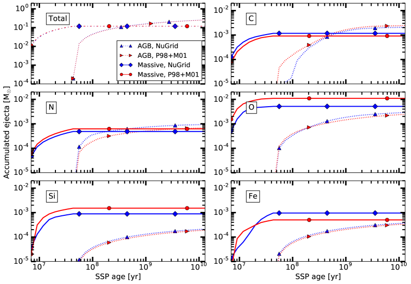
Figure 3: Accumulated ejecta of AGB stars and massive stars based on NuGrid yields and M01P98 yields, for an SSP of $1\,M_{\odot}$ at $Z=0.02$.

We compare the ejecta of two SSPs based on the yield set NuGrid_d yield set M01P98. Applied are NuGrid yields at $Z=0.02$, P98 yields at $Z=0.02$ and M01 yields at $Z=0.019$ which we will refer to as yields at solar metallicity. The initial abundances of the NuGrid yield set are selected. We calculate the total yields $y_{\rm tot}$ from the net yield set M01P98 (Sec. 2.1.5). We modified the M01P98 massive star yields by the factors 0.5, 2 and 0.5 for C, Mg, and Fe, respectively, as done in W09. Those modifications are justified in Appendix A3.2 of W09 and are applied in our work to provide a consistent comparison with the results of W09.

In this section we use identical SSP parameters (Table 2) to identify the differences due to different yield sets from M01P98 and NuGrid. $M_{\rm mass}$ represents the initial stellar mass that marks the transition between AGB and massive stars. We choose $M_{\rm mass}$ in agreement with the upper limit of the progenitors of SNe Ia applied in the SSP code (Sect. 2.1.3). The evolution of the total accumulated mass of AGB stars and massive stars is about the same for NuGrid yields and M01P98 yields due similar amounts of total ejecta of both yield sets.

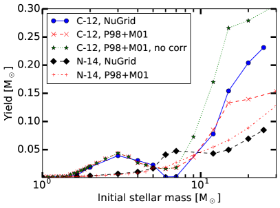
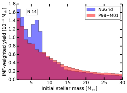
Figure 4: [12]C and [14]N yields at solar metallicity versus initial mass of NuGrid, M01P98 and M01P98 without correction factor (no corr) of 0.5 (left). IMF-weighted yields of [14]N of stars of different initial mass (right).

C, N

AGB stars are important sites of dust production (e.g. Ferrarotti & Gail, 2006; Schneider et al., 2014) and feature the primary production of C (Herwig, 2005). In massive and super-AGB stars C is transformed into N in hot-bottom burning (HBB) in the AGB stage (Lattanzio et al., 1996). The TP-AGB phase changes dramatically the structure and chemistry of intermediate mass models. Lower C yields in the NuGrid stellar models of $M_{\rm ZAMS}=6\,M_{\odot}$ and $M_{\rm ZAMS}=7\,M_{\odot}$ compared to stellar models of lower initial mass is due to more efficient [12]C destruction in the CNO cycle during HBB. The stellar models with $M_{\rm ZAMS}=6\,M_{\odot}$ and $M_{\rm ZAMS}=7\,M_{\odot}$ by P98 do not include the TP-AGB phase, the third dredge-up (TDUP) and destruction of C during HBB. The accumulated ejecta of [12]C of the SSP with M01P98 yields is higher than with NuGrid yields before $\approx 2\times 10^{8}\,\mathrm{yr}$ (Figure 3).

While the total SSP ejecta of C from AGB stars are 11% lower for NuGrid yields than for M01P98 yields, for massive stars total SSP ejecta are 30% larger. The massive stars of the SSP with NuGrid yields produce at all times more C than those of the SSP with M01P98 yields. Without the decrease of massive star yields of P98 by 0.5 as in this work and in W09 M01P98 yields would produce the most C. In the latter case AGB stars would start to dominate the total production of C at $9\times 10^{8}\,\mathrm{yr}$ instead of $3.6\times 10^{8}\,\mathrm{yr}$.

HBB transforms [12]C into [14]N, leading to larger stellar yields of N from NuGrid compared to the models of M01P98 (Figure 4). The result is a bump in the IMF-weighted ejecta of stellar models with $M_{\rm ZAMS}=6\,M_{\odot}$ and $M_{\rm ZAMS}=7\,M_{\odot}$. AGB stars based on NuGrid yields eject in total 28% more N than those with M01P98 yields. For massive stars it is 18% less N with NuGrid yields compared to M01P98 yields.

O, Si

Most O is produced in massive stars (Timmes et al., 1995; Woosley et al., 2002). Larger O shells for more massive stars do not necessarily lead to larger amounts of O ejected when strong fallback is taken into account. In stellar models with $M_{\rm ZAMS}=20\,M_{\odot}$ and $M_{\rm ZAMS}=25\,M_{\odot}$ from NuGrid strong fallback of large parts of the O shell results in larger remnant masses and less O ejection at high initial mass compared to P98 (Figure 5). This results in 47% lower O ejecta of the SSP than compared to the SSP with M01P98 yields (Figures 5 and 3).

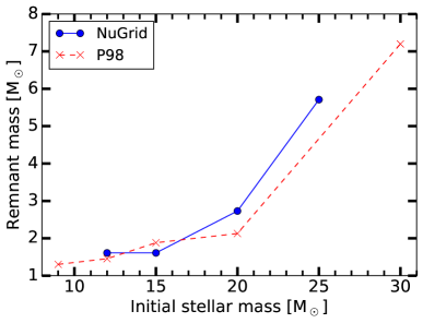
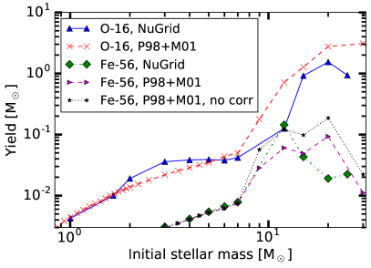
Figure 5: Remnant masses versus initial mass of NuGrid and P98 models at solar metallicity (left). Yields of O represented by [16]O and Fe yields represented by [56]Fe at solar metallicity versus initial mass (right).

AGB models of NuGrid include convective boundary mixing, which results in He-intershell enrichment of O of about 15% in low-mass TP-AGB models compared to 2% without any convective boundary mixing (Herwig, 2005). M01 do not include any convective boundary mixing which is why the mass of O from AGB stars is higher with NuGrid yields than with M01 yields. We find that the effect of convective boundary mixing on the total AGB production of O is small: the difference in SSP ejecta between NuGrid yields and M01 yields is only 17% (Figure 3).

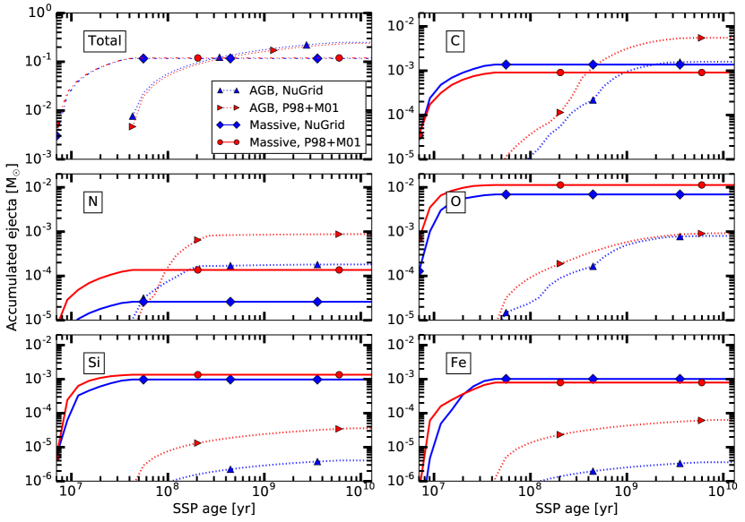
Figure 6: Accumulated ejecta of AGB stars and massive stars based on NuGrid yields at $Z=0.001$ and M01P98 yields at $Z=0.004$, for an SSP of $1\,M_{\odot}$.

Si is produced in massive stars (e.g. Timmes et al., 1995). Due to its closer proximity to the core than lighter elements the difference in chemical evolution of Si according to NuGrid and M01P98 yields are only slightly smaller than for O. 43% less Si is ejected with NuGrid yields than with yields of M01P98. AGB stars eject mostly unprocessed Si and the total amount ejected is within 10% between the yield sets.

Fe

The SSP ejecta of Fe of massive stars are qualitatively different between the yield sets (Figure 3) due to the variation of Fe yields with initial mass (Figure 5). This is primarily a consequence of the NuGrid remnant mass and fallback model adopted in this version of the NuGrid yields (Ritter et al., 2017). As a result Fe ejecta are two times larger for the $12\,M_{\odot}$ model compared to the $15\,M_{\odot}$ model at $Z=0.02$ and the $20$ and $25\,M_{\odot}$ models have further reduced Fe yields. M01P98 Fe yields peak, instead, at $M_{\rm ZAMS}=20\,M_{\odot}$. In cases like Fe, where the NuGrid yields predict a substantial rise toward the transition mass to white dwarf formation, the choice of interpolation vs. extrapolation of yields can be quite relevant. Our approach is described in Sect. 2.1.5. Ultimately, a higher model density at low masses would be the best solution. However, the lowest mass massive star models are the most difficult to calculate and are still subject to many modeling uncertainties. At later times the SSP ejecta of Fe from massive stars based on NuGrid yields are larger and the total ejecta based on NuGrid is 47% larger than the one based on M01P98 yields. SSP ejecta of Fe of AGB stars is unprocessed and its total amount ejected is within 10% between yield sets.

3.2 Simple Stellar Populations at Low Metallicity

To analyze the SSP ejecta at low metallicity we compare the yield set NuGrid_d at $Z=0.001$ with the yield set M01P98 at $Z=0.004$. To calculate the total yields from M01P98 (see Sect. 2.1.5), we used the initial abundance adopted for NuGrid models at solar Z but scaled down to $Z=0.004$. Yields of both sets at the same sub-solar metallicity are not available. The initial abundance of NuGrid yields at $Z=0.001$ is $\alpha$-enhanced in contrast to P98 and M01. We compare the total accumulated ejecta of AGB stars and massive stars based on yields from M01P98 with those based on NuGrid yields (Figure 6).

C, N

The total SSP ejecta of C from AGB stars is 71% lower with NuGrid yields compared to yields of M01P98 (Figure 6). This is due to the low-mass AGB models of P98 which eject larger amounts of C compared to NuGrid models (Figure 7). M01 use synthetic models which do not model the TDUP self-consistently contrary to the NuGrid models. In the synthetic models the dredge up of C into the envelope results from the calibration of the dredge-up strength and minimum core mass of TDUP occurrence against the observed carbon star luminosity distribution. The total SSP ejecta of C of massive stars is with NuGrid yields 37% higher than with M01P98 yields.

The total AGB ejecta of N of the SSP based on NuGrid yields is 80% lower than the N ejecta based on M01P98 yields. We find large discrepancies between N yields from NuGrid and yields of M01 for massive AGB models (Figure 7). The amounts of N produced in these stellar models during HBB depend on the length of the TP-AGB phase which is based on free parameters of the synthetic models of M01. The mass loss model adopted in the NuGrid simulations does also include an uncertain efficiency parameter. N yields in the NuGrid models are a result of convective boundary mixing assumptions and the modeling of the third dredge-up (see Ritter et al., 2017, for details). The SSP ejecta of N of massive stars with NuGrid yields is for most of the evolution 80% lower than with yields by M01P98.

O, Si

The stellar yields of O from AGB models differ more between the yield sets at lower metallicity than at solar metallicity. The difference is the largest for the most massive AGB models. This translates in a large difference of AGB ejecta of the SSPs early on in the evolution (Figure 6). With NuGrid yields the total amount of O ejected by AGB stars is 12% below the amount ejected with M01P98 yields. The evolution of SSP ejecta of O from massive stars is in slightly better agreement between the yield sets at low metallicity than at solar metallicity. The total SSP ejecta of O of massive stars with NuGrid yields is 39% lower than with M01P98 yields.

There is little SSP ejecta of Si from AGB stars. The difference between M01P98 and NuGrid yields in the Si ejecta is due to the different initial abundances of the stellar models. NuGrid adopts an $\alpha$-enhanced initial abundance for models of $Z=0.001$. When we apply the same initial abundance of Si AGB ejecta of both sets are in good agreement. The SSP ejecta of Si from massive stars are similar for the yield sets as at solar metallicity. We find a 28% lower total amount of Si ejected by massive stars of NuGrid compared to M01P98.

Fe

As for Si, the Fe ejecta from AGB stars based on NuGrid yields are lower than with M01P98 yields due to the adopted initial abundances. SSP ejecta of Fe of massive stars based on NuGrid yields starts below and then increases above the ejecta based on M01P98 yields. The strong fallback in NuGrid models of high initial mass limits the Fe ejecta at early times in the SSP evolution. The total amount of Fe ejected is 23% larger with NuGrid yields than with M01P98 yields.

3.3 Impact of Core-collapse Mass-cut Prescriptions

One of the major uncertainties in calculating yields for SSPs is the treatment of fallback after supernova explosions. NuGrid provides two explosion prescriptions based on the convective-enhanced neutrino-driven engine. (e.g. Fryer & Young, 2007; Fryer et al., 2012, F12). The rapid and delayed explosion assumptions refer to the case where a short and long time are needed for the convective engine to revive the shock. Accordingly, delayed explosions have generally more time for fallback and larger remnants, and rapid explosions have smaller remnants. The SSP ejecta of C, O and Si differ more between the fallback prescriptions at $Z=0.02$ than at $Z=0.001$ due to the BH formation after the rapid explosion of the stellar model with $M_{\rm ZAMS}=25\,M_{\odot}$ at $Z=0.001$ (see Ritter et al., 2017, for details) which prevents the ejection of the Si, O and C shell (Figure 8).

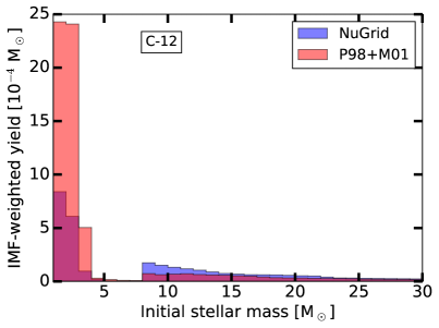
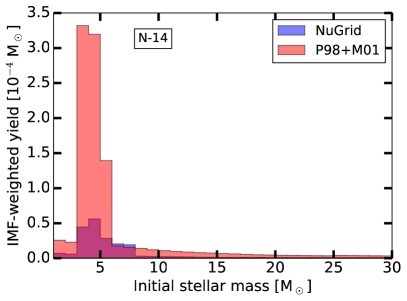
Figure 7: IMF-weighted yields of C represented by [12]C and N represented by [14]N versus initial mass based on NuGrid yields with $Z=0.001$ and M01P98 yields with $Z=0.004$, for an SSP of $1\,M_{\odot}$.

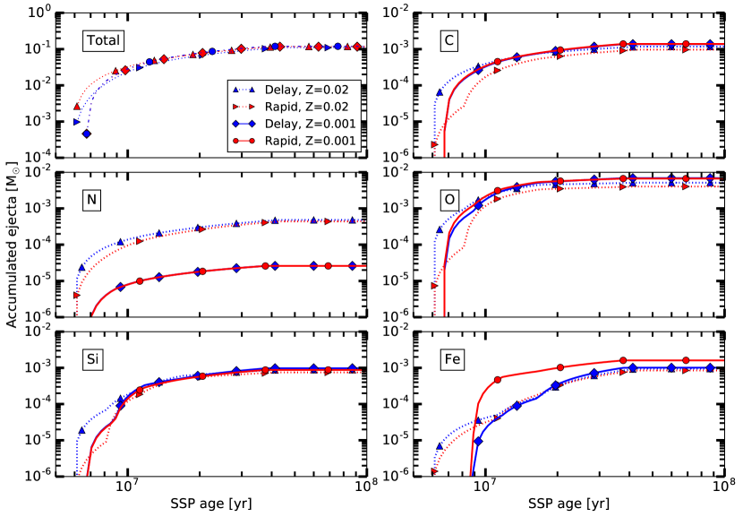
Figure 8: Accumulated ejecta of massive stars of NuGrid yields at $Z=0.02$ and $Z=0.001$ computed with the delayed and rapid CCSN fallback prescription, for an SSP of $1\,M_{\odot}$.

For the lower metallicity case the Fe ejection is larger for the rapid explosion as more Fe falls back in the delayed explosion case. Within the first $1.3\times 10^{7}\,\mathrm{yr}$ ten times more Fe is ejected with the rapid explosion compared to the delayed explosion. The expected range of explosion delay times (F12) could lead to large variations in Fe enrichment in the early universe.

The rapid explosion models match the observed gap between NS and BH remnants better than the delayed models even though the gap might be sparsely populated (F12 and references therein). Delayed explosions produce more fallback BHs, in particular at low mass and yield a larger fraction of low-mass BHs formed with a SN explosion. The latter can explain the observed BH systems which indicate a natal kick (F12). Fallback is also relevant to produce the weak supernova (Valenti et al., 2009) which are believed to be observed (F12). We recommend yields with the delayed explosion prescription in chemical evolution models. However, both cases may be necessary to explain all SN observations (F12). Therefore NuGrid offers yield tables that contain a half and half mixture of rapid and delayed options.

4 Summary and Conclusions

SYGMA provides the chemical ejecta and stellar feedback of simple stellar populations for application to galactic chemical evolution, hydrodynamical simulations and semi-analytical models of galaxies. A variety of SNIa delay-time distributions, IMF and yield options are included. SYGMA includes various non-standard nucleosynthesis sources, such as NS mergers and CCSN neutrino-driven winds, and can track the corresponding r-process enrichment. Along with the built-in plotting and analysis tools and the online web-accessible version (Appendix B) SYGMA can be used to trace cumulative features of GCE models to individual nuclear astrophysics properties of individual stellar models. SYGMA is part of the NuGrid Pyhon Chemical Evolution Environment NuPyCEE and consitutes a key building block in the JINA-NuGrid chemical evolution pipeline (e.g. Côté et al., 2017b, a) that integrates fundamental stellar and nuclear physics investigations with galactic modeling applications.

The primary focus of SYGMA is on investigating and applying the present and future NuGrid yields that are calculated using the same simulation tools and – as much as possible and appropriate – physics assumptions for low-mass and massive star models that are based on stellar evolution calculations and comprehensive nucleosynthesis simulations. Large, unquantifiable uncertainties that originate from the application of different AGB and massive star yield sets are avoided. Stellar feedback from CCSNe is consistent with the underlying explosion models of the NuGrid data set. Stellar luminosities in energy bands are calculated from time-dependent synthetic spectra of NuGrid stellar models. SYGMA tracks an arbitrary number of elements and isotopes up to Bi as provided by the NuGrid yields.

NuGrid yield tables are part of the larger NuPyCEE yield library which also includes a number of other yield sets from the literature, as well as yields from more exotic sources, such as MHD jets (Nishimura et al. 2015), hypernovae (Kobayashi et al. 2006), and NS mergers (Rosswog et al. 2014). Additional tables can be added on request.

A comparison of SSPs using NuGrid yields and the combined yields of P98 and M01 expose differences for C and N ejecta due to massive and super-AGB star yields and are the largest at low metallicity with a factor of 3.5 and 4.8. Different CCSN fallback treatments result in differences in C, O and Si of up to a factor of ten in certain cases, such as the first $10^{7}\mathrm{yr}$ of an SSP at $Z=0.001$ are possible. The largest difference of the total ejecta between the fallback prescriptions is for Fe with a factor 1.6. A brief code comparison of SYGMA with the W09 SSP code demonstrates the code design and implementation impact (Sect. A).

The functionality of the module was verified through a comparison with W09 in which we apply their yields. The final accumulated ejecta are well in agreement in both works and the largest differences in the fraction of ejecta of N and Fe from massive stars is 10%.

Appendix A Code verification

We compare SYGMA results calculated with the same yields as W09 (M01P98) with the W09 results. This serves two goals. The first is simply code verification. The second is to provide some estimate on the kinds of uncertainties that are introduced by small code design and implementation differences, which are in addition to the uncertainties in the yield input data. We choose for this comparison the widely used W09 work, but would expect to find similar outcomes when comparing with other SSP codes. As this appendix shows, the differences are small but not entirely insiginficant. Our response to these differences is to make our code public so that all code design and implementation details can be scrutinized, and changed if deemed appropriate.

We apply the same massive star model factors of 0.5, 2 and 0.5 as in W09, initial abundances from Table 1 of W09, and – as much as possible – the same chemical evolution parameters (Table 2). The initial mass range for which yields were ejected is not given W09 and we choose the range from $M_{\rm ZAMS}=0.8\,M_{\odot}$ to $M_{\rm ZAMS}=100\,M_{\odot}$ to match best Fig. 2 in W09.

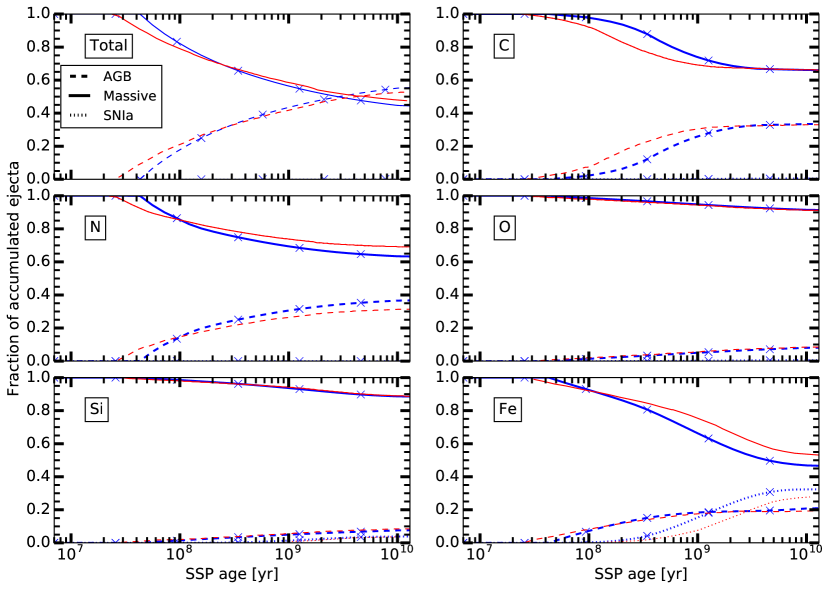
Figure 9: Fraction of total mass ejected from AGB, massive star and SNe Ia for a SSP at solar metallicity with yield input from M01P98 (blue, crosses) compared to results extracted from Fig. 2 in W09 (red). Results are based on the same yield input but different SSP codes.

Another important parameter is the transition initial mass $M_{\rm mass}$ that delineates white dwarf and supernova outcomes. It is not given in W09, but must be between $M_{\rm ZAMS}=7$ and $9\,M_{\odot}$ in the M01P98 set. The actual value of $M_{\rm mass}$ is still a matter of some debate (Poelarends et al., 2008; Doherty et al., 2015, 2017; Jones et al., 2016). For this section we have adopted a value (Table 2) that agrees best with the results shown in Fig. 2 of W09.

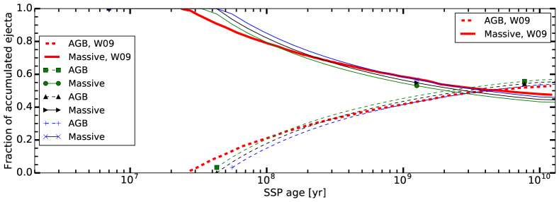
Figure 10: Evolution of fraction of total ejecta for transition masses of $M_{\rm ZAMS}=7.5\,M_{\odot}$, $M_{\rm ZAMS}=8\,M_{\odot}$ and $M_{\rm ZAMS}=8.5\,M_{\odot}$.

Overall the SYGMA and W09 SSP models agree well, but differences can be seen as low- and intermediate mass stars start to contributed – especially for C (up to $10\%$ differnce) and Fe (Figure 9). The choice of the transition mass $M_{\rm mass}$ determines the appearance of the AGB star ejecta and the drop in total massive star ejecta (Figure 10). The N yields increase smoothly with initial mass which leads to a smooth increase of the SSP ejecta similar to W09. The differences in the C and N evolution could be due to different yield interpolation methods used in the initial mass transition region from AGB to massive stars.

Appendix B Online availability

The SYGMA web interface allows to simulate, analyse, and extract SSP ejecta which includes all stable elements and many isotopes up to Bi. We introduce the yield sets and parameters which are available within the web interface. Yields for AGB stars and massive stars can be selected from the NuGrid sets NuGrid_d/r/m (Table 1) SNIa yields are from Thielemann et al. (2003) and Pop III yields are from Heger & Woosley (2010). The available metallicities are $Z=0.02$, $0.01$, $0.006$, $0.001$ and $0.0001$, $0$. Yields are applied in the initial mass range from $1\,M_{\odot}$ to $30\,M_{\odot}$. Chemical evolution parameters such as IMF and SNIa DTD can be set.

SSP ejecta can be extracted in the form of tables which contain for each time step the fraction of elements and isotopes of choice. As an example parts of a table which contains the normalized mass of elements ejected over $10^{10}\,\mathrm{yr}$ by a SSP of $1\,M_{\odot}$ at $Z=0.02$ is presented in Table 3.

Table 3: Sample of a table including time evolution of the ejected elements extracted with the SYGMA web interface, for a SSP of $1\,M_{\odot}$ at $Z=0.02$.

Age [yr]	C	N	O	Fe	Sr	Ba	Mtot [$\,M_{\odot}$]
1.000E+07	3.921E-04	1.391E-04	2.118E-03	4.179E-05	1.268E-08	7.086E-10	3.273E-02
……
1.000E+08	1.208E-03	8.412E-04	5.497E-03	1.025E-03	3.713E-08	3.192E-09	1.642E-01
……
1.000E+09	2.629E-03	1.212E-03	7.025E-03	1.301E-03	5.625E-08	7.224E-09	2.793E-01
……
1.000E+10	3.257E-03	1.408E-03	8.052E-03	1.655E-03	6.211E-08	9.051E-09	3.691E-01

The SYGMA code and the yield library can be accessed via http://nugrid.github.io/NuPyCEE. We provide an online documentation based on SPHINX, guides and teaching material in form of Jupyter notebooks. SYGMA web interface is accessible through the NuPyCEE web page and hosted on NuGrid’s Web Exploration of NuGrid Datasets: Interactive (WENDI) platform at http://wendi.nugridstars.org. WENDI is a Cyberhubs service (Herwig et al., 2018). Access to the figures of this work are provided through WENDI. NuGrid’s stellar and nucleosynthesis data sets are available at http://nugridstars.org/data-and-software/yields/set-1 and can be analyzed with WENDI.

References

- Abbott (1978) Abbott, D. C. 1978, ApJ, 225, 893
- Arnett (1996) Arnett, D. 1996, Supernovae and Nucleosynthesis
- Arnett et al. (1989) Arnett, W. D., Bahcall, J. N., Kirshner, R. P., & Woosley, S. E. 1989, ARA&A, 27, 629
- Arnould et al. (2007) Arnould, M., Goriely, S., & Takahashi, K. 2007, Phys. Rep., 450, 97
- Audouze & Tinsley (1976) Audouze, J., & Tinsley, B. M. 1976, ARA&A, 14, 43
- Bolton (2000) Bolton, C. T. 2000, Physics Today, 53, 48
- Castelli & Kurucz (2004) Castelli, F., & Kurucz, R. L. 2004, ArXiv Astrophysics e-prints, astro-ph/0405087
- Chabrier (2003) Chabrier, G. 2003, PASP, 115, 763
- Côté et al. (2015) Côté, B., Martel, H., & Drissen, L. 2015, ApJ, 802, 123
- Côté et al. (2017a) Côté, B., O’Shea, B. W., Ritter, C., Herwig, F., & Venn, K. A. 2017a, ApJ, 835, 128
- Côté et al. (2017b) Côté, B., Ritter, C., Herwig, F., et al. 2017b, in 14th International Symposium on Nuclei in the Cosmos (NIC2016), ed. S. Kubono, T. Kajino, S. Nishimura, T. Isobe, S. Nagataki, T. Shima, & Y. Takeda, 020203
- Côté et al. (2016) Côté, B., Ritter, C., O’Shea, B. W., et al. 2016, ApJ, 824, 82
- Côté et al. (2018) Côté, B., Silvia, D. W., O’Shea, B. W., Smith, B., & Wise, J. H. 2018, ApJ, 859, 67
- Cristallo et al. (2015) Cristallo, S., Straniero, O., Piersanti, L., & Gobrecht, D. 2015, ApJS, 219, 40
- Dahlen et al. (2004) Dahlen, T., Strolger, L.-G., Riess, A. G., et al. 2004, ApJ, 613, 189
- Doherty et al. (2017) Doherty, C. L., Gil-Pons, P., Siess, L., & Lattanzio, J. C. 2017, ArXiv e-prints, arXiv:1703.06895 [astro-ph.SR]
- Doherty et al. (2015) Doherty, C. L., Gil-Pons, P., Siess, L., Lattanzio, J. C., & Lau, H. H. B. 2015, MNRAS, 446, 2599
- Dominik et al. (2012) Dominik, M., Belczynski, K., Fryer, C., et al. 2012, ApJ, 759, 52
- Ferrarotti & Gail (2006) Ferrarotti, A. S., & Gail, H.-P. 2006, A&A, 447, 553
- Few et al. (2012) Few, C. G., Courty, S., Gibson, B. K., et al. 2012, MNRAS, 424, L11
- Few et al. (2014) Few, C. G., Courty, S., Gibson, B. K., Michel-Dansac, L., & Calura, F. 2014, MNRAS, 444, 3845
- Fryer et al. (2012) Fryer, C. L., Belczynski, K., Wiktorowicz, G., et al. 2012, ApJ, 749, 91
- Fryer & Young (2007) Fryer, C. L., & Young, P. A. 2007, ApJ, 659, 1438
- Gibson (1995) Gibson, B. K. 1995, PhD thesis, THE UNIVERSITY OF BRITISH COLUMBIA (CANADA).
- Gibson (1997) —. 1997, MNRAS, 290, 471
- Gibson (2002) Gibson, B. K. 2002, in IAU Symposium, Vol. 187, Cosmic Chemical Evolution, ed. K. Nomoto & J. W. Truran, 159
- Heger & Woosley (2010) Heger, A., & Woosley, S. E. 2010, ApJ, 724, 341
- Herwig (2005) Herwig, F. 2005, Annual Review of Astronomy and Astrophysics, 43, 435
- Herwig et al. (2018) Herwig, F., Andrassy, R., Annau, N., et al. 2018, ApJS, 236, 2
- Hopkins et al. (2012) Hopkins, P. F., Quataert, E., & Murray, N. 2012, MNRAS, 421, 3522
- Husser et al. (2013) Husser, T.-O., Wende-von Berg, S., Dreizler, S., et al. 2013, A&A, 553, A6
- Iwamoto et al. (1999) Iwamoto, K., Brachwitz, F., Nomoto, K., et al. 1999, ApJS, 125, 439
- Jones et al. (2016) Jones, S., Ritter, C., Herwig, F., et al. 2016, MNRAS, 455, 3848
- Karakas et al. (2010) Karakas, A. I., Campbell, S. W., & Stancliffe, R. J. 2010, ApJ, 713, 374
- Kawata & Gibson (2003) Kawata, D., & Gibson, B. K. 2003, MNRAS, 340, 908
- Kobayashi et al. (2006) Kobayashi, C., Umeda, H., Nomoto, K., Tominaga, N., & Ohkubo, T. 2006, ApJ, 653, 1145
- Kroupa (2001) Kroupa, P. 2001, MNRAS, 322, 231
- Kroupa et al. (2013) Kroupa, P., Weidner, C., Pflamm-Altenburg, J., et al. 2013, in Planets, Stars and Stellar Systems. Volume 5: Galactic Structure and Stellar Populations, ed. T. D. Oswalt & G. Gilmore, 115
- Lattanzio et al. (1996) Lattanzio, J., Frost, C., Cannon, R., & Wood, P. R. 1996, Mem. Soc. Astron. Italiana, 67, 729
- Leitherer et al. (1992) Leitherer, C., Robert, C., & Drissen, L. 1992, ApJ, 401, 596
- Leitherer et al. (1999) Leitherer, C., Schaerer, D., Goldader, J. D., et al. 1999, ApJS, 123, 3
- Mannucci et al. (2006) Mannucci, F., Della Valle, M., & Panagia, N. 2006, MNRAS, 370, 773
- Maoz & Mannucci (2012) Maoz, D., & Mannucci, F. 2012, PASA, 29, 447
- Marigo (2001a) Marigo, P. 2001a, A&A, 370, 194
- Marigo (2001b) —. 2001b, A&A, 370, 194
- Nishimura et al. (2015) Nishimura, N., Takiwaki, T., & Thielemann, F.-K. 2015, ApJ, 810, 109
- Nomoto et al. (2013) Nomoto, K., Kobayashi, C., & Tominaga, N. 2013, ARA&A, 51, 457
- Pagel (2009) Pagel, B. E. J. 2009, Nucleosynthesis and Chemical Evolution of Galaxies (Cambridge University Press)
- Pignatari et al. (2016) Pignatari, M., Herwig, F., Hirschi, R., et al. 2016, ApJS, 225, 24
- Poelarends et al. (2008) Poelarends, A. J. T., Herwig, F., Langer, N., & Heger, A. 2008, apj, 675, 614
- Portinari et al. (1998) Portinari, L., Chiosi, C., & Bressan, A. 1998, A&A, 334, 505
- Ritter & Côté (2016) Ritter, C., & Côté, B. 2016, NuPyCEE: NuGrid Python Chemical Evolution Environment, Astrophysics Source Code Library, ascl:1610.015
- Ritter et al. (2018) Ritter, C., Côté, B., Paul, A., & Herwig, F. 2018, NuGrid/NuPyCEE: NuPyCEE in Python 3
- Ritter et al. (2017) Ritter, C., Herwig, F., Jones, S., et al. 2017, ArXiv e-prints, arXiv:1709.08677 [astro-ph.SR]
- Romano et al. (2010) Romano, D., Karakas, A. I., Tosi, M., & Matteucci, F. 2010, A&A, 522, A32
- Rosswog et al. (2014) Rosswog, S., Korobkin, O., Arcones, A., Thielemann, F.-K., & Piran, T. 2014, MNRAS, 439, 744
- Rybizki et al. (2017) Rybizki, J., Just, A., & Rix, H.-W. 2017, A&A, 605, A59
- Saitoh (2017) Saitoh, T. R. 2017, AJ, 153, 85
- Salpeter (1955) Salpeter, E. E. 1955, ApJ, 121, 161
- Schneider et al. (2014) Schneider, R., Valiante, R., Ventura, P., et al. 2014, MNRAS, 442, 1440
- Seitenzahl et al. (2013) Seitenzahl, I. R., Ciaraldi-Schoolmann, F., Röpke, F. K., et al. 2013, MNRAS, 429, 1156
- Somerville & Davé (2015) Somerville, R. S., & Davé, R. 2015, ARA&A, 53, 51
- Thielemann et al. (1986) Thielemann, F.-K., Nomoto, K., & Yokoi, K. 1986, Astronomy and Astrophysics, 158, 17
- Thielemann et al. (2003) Thielemann, F.-K., Argast, D., Brachwitz, F., et al. 2003, in From Twilight to Highlight: The Physics of Supernovae, ed. W. Hillebrandt & B. Leibundgut, 331
- Timmes et al. (1995) Timmes, F. X., Woosley, S. E., & Weaver, T. A. 1995, APJS, 98, 617
- Valenti et al. (2009) Valenti, S., Pastorello, A., Cappellaro, E., et al. 2009, Nature, 459, 674
- Van Der Walt et al. (2011) Van Der Walt, S., Colbert, S. C., & Varoquaux, G. 2011, ArXiv e-prints, arXiv:1102.1523 [cs.MS]
- Wiersma et al. (2009) Wiersma, R. P. C., Schaye, J., Theuns, T., Dalla Vecchia, C., & Tornatore, L. 2009, Monthly Notices of the Royal Astronomical Society, 399, 574
- Woosley et al. (2002) Woosley, S. E., Heger, A., & Weaver, T. A. 2002, Rev. Mod. Phys., 74, 1015
- Woosley & Weaver (1995) Woosley, S. E., & Weaver, T. A. 1995, APJS, 101, 181