Galaxy And Mass Assembly (GAMA): the G02 field, Herschel-ATLAS target selection and Data Release 3

Abstract

We describe data release 3 (DR3) of the Galaxy And Mass Assembly (GAMA) survey. The GAMA survey is a spectroscopic redshift and multi-wavelength photometric survey in three equatorial regions each of 60.0 deg² (G09, G12, G15), and two southern regions of 55.7 deg² (G02) and 50.6 deg² (G23). DR3 consists of: the first release of data covering the G02 region and of data on H-ATLAS sources in the equatorial regions; and updates to data on sources released in DR2. DR3 includes 154 809 sources with secure redshifts across four regions. A subset of the G02 region is 95.5% redshift complete to $r<19.8\,\mathrm{mag}$ over an area of $19.5\,{\rm deg}^{2}$, with 20 086 galaxy redshifts, that overlaps substantially with the XXL survey (X-ray) and VIPERS (redshift survey). In the equatorial regions, the main survey has even higher completeness ($98.5$%), and spectra for about 75% of H-ATLAS filler targets were also obtained. This filler sample extends spectroscopic redshifts, for probable optical counterparts to H-ATLAS sub-mm sources, to 0.8 mag deeper ($r<20.6\,\mathrm{mag}$) than the GAMA main survey. There are 25 814 galaxy redshifts for H-ATLAS sources from the GAMA main or filler surveys. GAMA DR3 is available at the survey website (www.gama-survey.org/dr3/).

1 Introduction

Modern day surveys designed to study galaxy evolution typically combine data from many wavelength regimes. Often this starts out with an optical imaging or spectroscopic survey, which can be a wide field or a deep-small field, and other instruments follow suit adding to the available data that can be combined. This is useful because different phenomena dominate at different wavelengths: young stars in the UV, older stars in the near-IR, dust emission in the far-IR, AGN-driven jets in the radio, and hot gas around AGN or in clusters of galaxies in the X-ray bands. Investigating the connections between these and other phenomena is enabled by a multi-wavelength approach (e.g. Jannuzi & Dey 1999; Dickinson & Giavalisco 2003; Scoville et al. 2007; Driver et al. 2016).

With the advent of wide-field imagers at the European Southern Observatory, OmegaCAM on the VST (Kuijken et al., 2002) and the VISTA Infrared Camera (Dalton et al., 2006), large public surveys were sought. One of these, KiDS using the VST, was approved to cover $1500\,{\rm deg}^{2}$ (de Jong et al., 2013). The chosen sky areas covered the 2dFGRS (Colless et al., 2001) in the south and the 2dFGRS and SDSS (Stoughton et al., 2002) near the celestial equator for their spectroscopic redshifts. The 2dFGRS areas were originally chosen for low Galactic extinction, i.e. in the Galactic caps, and for all year access from the AAT. The VIKING survey (Edge et al., 2013) was designed to cover the same area of sky as KiDS. VIKING observations are now complete, over a final area of $1350\,{\rm deg}^{2}$, and KiDS will cover the same area, i.e. 90% of the original aim.

In 2007, the GAMA survey was selected as a large-programme galaxy redshift survey on the AAT, using an update to the 2dF spectrograph called AAOmega (Sharp et al., 2006). The motivations included an aim for high redshift completeness to $r<19.8\,\mathrm{mag}$ for reliably selecting groups of galaxies to measure the halo mass function, and for a general purpose study of galaxy evolution using multi-wavelength data (Driver et al., 2009). The areas chosen were primarily within the KiDS footprint with GAMA regions now known as G09, G12 and G15 straddling the equator, and starting later, G23 in the south (see Table 1 for details of the GAMA regions). These four regions were also chosen to be observed with the Herschel Space Observatory, in the far-IR, as part of the H-ATLAS (Eales et al., 2010).

Table 1: Overview of the GAMA survey regions. The southern G02 and G23 regions were not part of GAMA I. The last column provides the magnitude limits for DR3, which was selected from GAMA II. The qualifier ‘GAMA II’ refers to the fact that a revised input catalogue was used for the second phase of the GAMA survey. See Baldry et al. (2010) for a detailed description of the GAMA I input catalogue and Liske et al. (2015) for a description of the changes to the input catalogue for GAMA II. Thus, I and II refer to two phases of target selection, and not the data releases, DR1, DR2, and DR3.

Survey region RA range (J2000) Declination range (J2000) Area main survey limits ($r$ band except in G23) (deg) (deg) (deg²) (mag) GAMA I GAMA II GAMA II GAMA I GAMA II DR3 G02 $30.2$  – $38.8$ – $-10.25$  – $-3.72$ $55.71$ – $19.8$ $19.8$ G09 $129.0$  – $141.0$ $-1.0$  – $+3.0$ $-2.0$  – $+3.0$ $59.98$ $19.4$ $19.8$ $19.0$ G12 $174.0$  – $186.0$ $-2.0$  – $+2.0$ $-3.0$  – $+2.0$ $59.98$ $19.8$ $19.8$ $19.0$ G15 $211.5$  – $223.5$ $-2.0$  – $+2.0$ $-2.0$  – $+3.0$ $59.98$ $19.4$ $19.8$ $19.8$ G23 $339.0$  – $351.0$ – $-35.0$  – $-30.0$ $50.59$ – $19.2$ ($i$ band) –

Unfortunate delays to VST meant that GAMA target selection was based on SDSS for the equatorial fields, and an additional GAMA field was sought and chosen, G02, to cover the CFHTLS-W1 field (Gwyn, 2012). The initial aim was to make use of the combined lensing maps from the CFHTLenS team (Heymans et al., 2012) and GAMA group catalogue (Robotham et al., 2011) based on a highly-complete redshift survey to $r<19.8\,\mathrm{mag}$. However, this GAMA region was not observed to a high level of redshift completeness except in an area that overlaps with the XXL survey, XXL-N field (Pierre et al., 2016). Thus, while the G02 region does not have the same homogeneous data set from the $u$-band to far-IR that have covered the other four regions (KiDS/VIKING/H-ATLAS), it has the largest area covered by XMM-Newton observations. Other surveys such as VIDEO (Jarvis et al., 2013) and HerMES (Oliver et al., 2012) cover some of the XXL-N field; and there are observations in the $K$-band with CFHT (Ziparo et al., 2016) and 3.6 and 4.5 $\mu$m with Spitzer (Lonsdale et al., 2003; Bremer et al., 2012).

The total sky area of the five GAMA regions is $286\,{\rm deg}^{2}$. The first and second data releases of the GAMA survey, as well as extensive survey diagnostics, are presented in Driver et al. (2011) and Liske et al. (2015). The target selection and the 2dF tiling strategy are described in Baldry et al. (2010) and Robotham et al. (2010), with spectroscopic reduction and redshift measurements described in Hopkins et al. (2013) and Baldry et al. (2014). Curation of and photometric measurements using the multi-wavelength imaging data, for the four regions excluding G02, are described in Driver et al. (2016).

In DR2, data products based on spectroscopic data or redshifts were released for targets down to $r<19.0\,\mathrm{mag}$ in G09 and G12, and $r<19.4\,\mathrm{mag}$ in G15. The aim of this paper is to describe the third data release of the GAMA survey. In addition to the DR2 targets, this includes: data from the G02 region; data on H-ATLAS selected targets regardless of magnitude; data on targets in G15 to $r<19.8\,\mathrm{mag}$; expanded areal coverage of the equatorial regions; and any updates to data products since DR2. The G02 data are described in § 2 and 3. The H-ATLAS target selection is described in § 4, GAMA-team data products are described in § 5, and a summary of DR3 is provided in § 6. Optical magnitudes were corrected for Galactic dust extinction using the maps of Schlegel et al. (1998).

2 G02 imaging

The G02 field is the region defined by $30.2<\mathrm{RA}<38.8$ and $-10.25<\mathrm{DEC}<-3.72$, which is a large subset, covering 87%, of the CFHTLS W1 field. As well as CFHTLS data, SDSS imaging covers most of the G02 field, and XXL covers about $25\,{\rm deg}^{2}$. The optical imaging surveys were used to define the target selection, while the XXL coverage was considered when defining the high completeness region. Figure 1 shows the G02 field with the boundaries of these and other surveys.

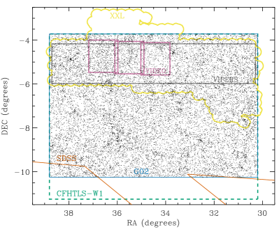
Figure 1: Location of the GAMA/G02 field. The blue line outlines the G02 region while the points represent the distribution of target galaxies to $r<19.8\,\mathrm{mag}$. The green dashed line outlines the CFHTLS-W1 field. The yellow line outlines the XXL region. The orange lines show the lower boundary of SDSS coverage. The pink rectangles outline the VISTA-VIDEO coverage. The black rectangle outlines the VIPERS coverage.

Imaging for the CFHTLS was taken using the CFHT MegaCam instrument (Boulade et al., 2003), which consists of 36 2048-by-4612 pixel CCDs. During a typical pointing with dithering to fill in the detector gaps, a contiguous area of $\sim 1\,{\rm deg}^{2}$ is observed. The W1 field was covered using 72 pointings, of which, 63 pointings were used for the G02 region. Observations were taken in five filters $u$, $g$, $r$, $i$, $z$ with typically 2000 s to 4000 s exposures, and with seeing FWHM typically between $0.5^{\prime\prime}$ and $1.0^{\prime\prime}$. We used the data products based on the processing by the CFHTLenS team described in Erben et al. (2013). Objects were detected using SExtractor (Bertin & Arnouts, 1996) on the $i$-band images, with multi-wavelength photometry obtained using the multi-image mode on PSF-matched images in all the bands (Hildebrandt et al., 2012). A mask was also supplied by the CFHTLenS team that removed satellite trails, optical ghosts, saturated pixels, diffraction spikes and other artefacts. An initial input catalogue of 317 748 sources was obtained by selecting all sources to r-band AUTO mag $<21$ that had not been masked.

The SDSS is a set of surveys using a 2.5-m telescope at Apache Point Observatory (York et al., 2000). Imaging for SDSS used a large format CCD camera in drift-scan mode with five broadband filters $u$, $g$, $r$, $i$ and $z$. The exposure time on source was 55 s during a normal drift-scan run. Gaps between the detectors were filled in by observing with another run offset in the orthogonal direction to the drift scan. The sources and multi-wavelength photometry were obtained using a custom-made pipeline for SDSS called photo (Stoughton et al., 2002). Here we use imaging data provided by SDSS DR8 (Aihara et al., 2011). An initial input catalogue of 490 292 sources was obtained using an SQL query to the SDSS database to Petrosian $r$-band mag $<21$ over a marginal superset region (30 to 39 in RA, $-12$ to $-2$ in DEC). No mask was applied but a standard set of flags were applied that effectively removes most artefacts in the imaging caused by bright stars.

3 G02 target selection

Targets were selected from both the CFHTLenS and SDSS DR8 input catalogues, described above, which were then merged. SDSS objects were matched to the nearest CFHTLenS object within a $2^{\prime\prime}$ matching radius. If an SDSS object did not have a counterpart in the CFHTLenS catalogue then a new object was added to the merged catalogue (e.g., this can happen for galaxies that were initially lost in the large CFHTLenS bright star halos). Objects could be selected for spectroscopic targeting using photometry from either input catalogue, whether or not they had photometry from one or both.

For the G02 main survey, galaxies with $r<19.8\,\mathrm{mag}$ after correction for Galactic dust extinction were targeted in G02. The type of magnitudes used, for this flux-limited selection, were SExtractor AUTO (Kron, 1980; Bertin & Arnouts, 1996) for CFHTLenS and Petrosian (Petrosian, 1976; Stoughton et al., 2002) for SDSS. These both use adaptive apertures. Other magnitudes used were $3^{\prime\prime}$-aperture (SDSS fibre-size) magnitudes, which help to exclude artefacts related to the adaptive apertures, PSF magnitudes and profile-fitted (PSF$+$model) magnitudes. The differences between the latter two magnitudes for each source was used by SDSS as a star-galaxy profile separator.

Galaxies were targeted if they met the $r<19.8$ criterion in either the CFHTLenS or SDSS input catalogues, with details below:

• For CFHTLenS, the selection criteria were objects with SExtractor $\mathrm{CLASS\_STAR}<0.70$ and $r_{\rm auto}<19.8\,\mathrm{mag}$. In addition: targets were required to have an r-band 12 pixel ($3^{\prime\prime}$, i.e., SDSS-size fibre) aperture magnitude in the range $17<r_{\rm fib}<22.5$; and data in masked regions were excluded, for example, around bright stars.

• For SDSS DR8, the selection criteria were galaxies with $r_{\rm Petro}<19.8\,\mathrm{mag}$. Star-galaxy separation for SDSS was done using the method outlined by Baldry et al. (2010), without the $J-K$ measurements, using a combination of $r$-band PSF and model magnitudes (Stoughton et al., 2002) as follows:

  $$r_{\rm psf}-r_{\rm model}>\begin{array}[]{l}0.25\\ 0.25-\frac{1}{15}(r_{\rm model}-19)\\ 0.15\end{array}\mbox{~{}for~{}}\begin{array}[]{l}r_{\rm model}<19.0\\ 19.0~{}~{}...~{}~{}20.5\\ r_{\rm model}>20.5\end{array}$$ (1)

  SDSS selected targets had an SDSS $r$-band fibre magnitude in the range $17<r_{\rm fib}<22.5$. A number of standard flags were also applied to exclude artefacts.

Filler targets were selected down to $r<20.2\,\mathrm{mag}$ (with lower priority) from both surveys using the same criteria, other than the change in magnitude limit, outlined above.

Data for the targets are given in the G02TilingCat table. Targets selected as part of the main survey can be identified using the G02 survey_class (SC) parameter. The SC parameter takes the values: 6 for main-survey targets selected from SDSS and CFHTLenS; 5, from SDSS only; 4, from CFHTLenS only; and 2 for filler targets selected from either. Visual classification was performed on a subset of $\mathrm{SC}\geq 4$ sources, particularly those with discrepant photometry between the two input catalogues, to identify artefacts, deblended parts of large galaxies and severely affected photometry. Based on these visual checks, 290 sources were given an SC value of zero to indicate that they were not a target. The number of remaining main survey ($\mathrm{SC}\geq 4$) targets in G02TilingCat is 59 285.

Figure 2 shows a comparison between the selection photometry from SDSS and CFHTLenS. There is in general good agreement between the two data sets, and photometric measurement codes, given the challenging problem of galaxy photometry. Users should be aware, however, that SC=5 and SC=4 sources dominate in certain areas of the G02 region as shown by Fig. 3. This is because some areas were masked by CFHTLenS and one corner did not have SDSS imaging.

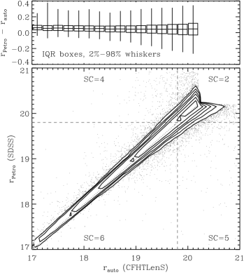
Figure 2: Comparison between the photometry from the two G02 input catalogues for sources that were identified as galaxy targets in both catalogues. The median value of $r_{\rm Petro}-r_{\rm auto}$ is 0.04 and the interquartile range (IQR) is 0.11. Note there is some variation in the median offset with position on the sky; this likely reflects variations in the CFHTLenS photometric calibration. The dashed lines divide the different survey_class regions.

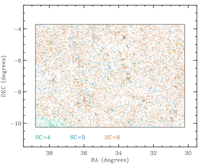
Figure 3: Sky distribution of G02 galaxy targets colour-coded according to survey_class. The SC=4 region at the bottom left of the plot corresponds to the region of G02 without SDSS coverage.

Spectra for the targets were obtained using the AAOmega/2dF instrument on the AAT, a multi-object fibre-fed spectrograph, excluding targets that already had a high-quality redshift from SDSS. For a single 2dF configuration (‘tile’), typically 350 fibres were allocated to targets and 25 fibres were allocated to positions for determining a mean sky background. The AAOmega dual-beam setup was chosen so that spectra were obtained from 3750Å to 8850Å with a dichroic split at 5700Å. The dispersion was 1Å per pixel in the blue arm and 1.6Å per pixel in the red arm. For an observation of a tile, data from usually three exposures and from each arm were combined such that a single sky-subtracted spectrum per target was obtained (Hopkins et al., 2013). The redshifts for each spectrum were then measured using a robust and reliability-calibrated cross-correlation method (Baldry et al., 2014).

The tiling strategy was similar to the GAMA equatorial regions (Robotham et al., 2010) with priorities from high-to-low for: main-survey targets that had not been observed spectroscopically, main-survey targets with one spectrum but no reliable redshift, quality-control targets, and filler targets. Clustered main-survey targets, defined as being within $40^{\prime\prime}$ of another main-survey target, were given a boosted priority. This helps with the strategy of obtaining high completeness, regardless of target density, with multiple visits because of the necessity in avoiding fibre collisions on any single visit.

Note that it became apparent during 2013 that the time allocated for the GAMA survey was not going to allow completion of the G02 region to a high completeness level. At this stage, it was decided to prioritise the overlap with the XXL survey. In the last season of observing, main-survey targets north of $-6.0\degr$ were given the highest priority though some targets between $-6.3\degr$ and $-6.0\degr$ were observed to avoid a hard edge in completeness. As a result of this, the redshift completeness is 95.5% for the main survey north of $-6.0\degr$, 46.4% between $-6.3\degr$ and $-6.0\degr$, and 31% south of $-6.3\degr$, on average. The redshift completeness is defined as the percentage of objects in a sample with reliable redshifts. Figure 4 shows a completeness map of the G02 region. Note that for the area south of $-6.0\degr$, the completeness is significantly higher for clustered targets compared to unclustered targets.

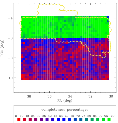
Figure 4: Map of the redshift completeness of the G02 field. The colour coding is according to the percentage of main-survey targets ($\mathrm{SC}\geq 4$) with a reliable redshift ($nQ\geq 3$) in areas of $0.2\degr\times 0.2\degr$. The yellow line outlines the XXL region.

It is clear that the $19.5\,{\rm deg}^{2}$ area north of $-6.0\degr$ has the fidelity required for a robust group catalogue and other clustering measurements, however, care must be taken to understand the effect of combined SDSS and CFHTLenS selection. There are 21 152 main-survey targets, of which 20 200 have a reliable redshift with $nQ\geq 3$ (completeness of 95.5%; $nQ$ is the redshift quality flag as defined in Liske et al. 2015). The completeness is 96.2% for main-survey targets that have a CFHTLenS $r$-band AUTO mag measurement. Figure 5 shows the magnitude distribution of targets and the redshift completeness versus $r_{\rm auto}$. The magnitude distribution is also shown divided according to source of redshift: SDSS or AAOmega, and in the latter case whether more than one spectrum was taken. This demonstrates that in order to obtain high completeness at the faint end, it is necessary to observe many of the targets twice. This can compensate for variable conditions and fibre throughput, as well as allowing coadding of two spectra to increase the signal-to-noise ratio.

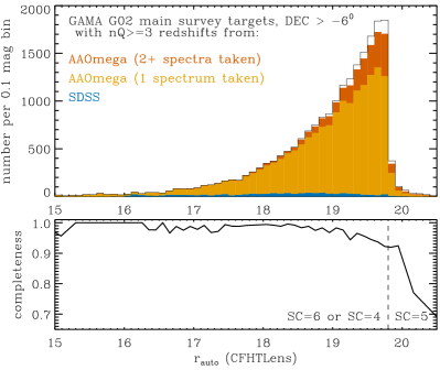
Figure 5: Magnitude distribution and redshift completeness of the main-survey targets in the G02 field north of $-6.0\degr$. The colour coding in the upper panel shows targets with reliable redshifts from SDSS and AAOmega, and whether or not more than one spectrum were taken for the GAMA survey. The main-survey targets to the right of the dashed line were selected because of their SDSS magnitudes (SC=5, see Fig. 2).

Figure 6 shows the redshift histogram of the GAMA-G02 high-completeness area. Also shown are the histograms for VIPERS (Garilli et al., 2014) and PRIMUS (Coil et al., 2011), which covers part of G02. VIPERS uses photo-$z$ selection to target galaxies at $z>0.5$, thus, there are almost no common targets between GAMA and VIPERS (which covers $\sim 15\,{\rm deg}^{2}$). In consideration of matching with XXL, for example, this leads to the situation where the structures are well defined by GAMA at $z<0.35$ and by VIPERS at $z>0.5$, with a redshift coverage gap. PRIMUS only fills this over a significantly smaller area. There are also 11 000 redshifts available from VVDS (Le Fèvre et al., 2013), not shown, over about $0.6\,{\rm deg}^{2}$ with a redshift interquartile range of 0.54–1.12.

Figure 6: Redshift histograms for the G02 area, ${\rm DEC}>-6.0\degr$, comparing GAMA (solid line), VIPERS (dashed line) and PRIMUS (dotted line). The bin spacing is 0.01 in $\ln(1+z)$.

The G02 group catalogue was constructed using the same code as presented in Robotham et al. (2011), primarily over the highly complete region of G02 (declination $>-6\degr$). To make use of the less complete redshifts available below declination $-6$, we made a hard cut at declination $>-6.3\degr$ but use $-6$ as the border flag within the group finding code. To be consistent with the GAMA equatorial regions, we use the SDSS $r_{\rm Petro}<19.8\,\mathrm{mag}$ selected targets only ($\mathrm{SC}\geq 5$). After redshift cuts, this results in 20 029 galaxies available for group finding. The resultant group catalogue has 2 540 ‘groups’ with two or more members. We compute the same standard group statistics as per Robotham et al. (2011), with the same halo mass and group luminosity calibrations.

It is important to note that the number of galaxies linked in each group, NFOF, does not have a physical meaning because it is defined using a magnitude-limited sample. Here, we compute the richness using a density-defining population (DDP) that has $M_{r}<-21\,\mathrm{mag}$. The richness ($N$) is the the number of DDP galaxies in a group. The absolute magnitude is given by

$$M_{r}=r_{\rm Petro}-5\log(D_{L}/10{\rm\,pc})-k_{r}+1.03z\mbox{~{}~{}~{},}$$ (2)

with k-corrections using kcorrect (Blanton & Roweis, 2007) and with an evolution factor of 1.03 from the $Q_{e}$ value derived by Loveday et al. (2015) (table 3 of their paper). Given the spectroscopic limit of $r<19.8\,\mathrm{mag}$, the DDP galaxies are volume limited to $z<0.28$, though we assume the richness values are reliable to $z<0.3$.

The number of ‘rich’ groups, $N\geq 5$, in the high-completeness G02 region (DEC $>-6$, $19.5\,{\rm deg}^{2}$), and in the redshift range $0.1<z<0.3$, is 98. This gives a number density of $3.0\times 10^{-5}\,\mathrm{Mpc}^{-3}$. This is higher than the average for the equatorial regions but consistent with cosmic variance. For the equatorial regions divided into nine $20\,{\rm deg}^{2}$ areas, the number density ranges from $2.1\times 10^{-5}\,\mathrm{Mpc}^{-3}$ to $3.4\times 10^{-5}\,\mathrm{Mpc}^{-3}$. Figure 7 shows the distribution of the G02 rich groups in RA and redshift as a ‘cone plot’.

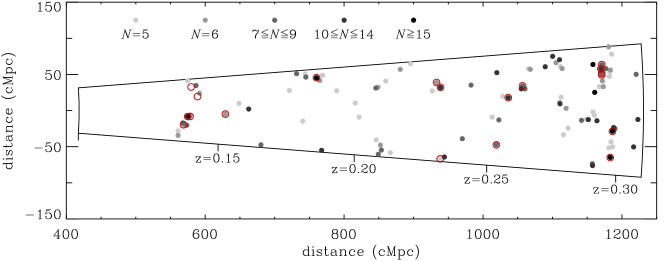
Figure 7: Cone plot of the GAMA groups in the G02 high-completeness region ($-6.0<{\rm DEC}<-3.72$, the two dimensions shown correspond to RA and redshift). The GAMA groups with richness $N\geq 5$ are shown with filled circles, shaded according to the number of galaxies with $M_{r}<-21\,\mathrm{mag}$. The XXL clusters from the bright cluster sample of Pacaud et al. (2016) are shown with red circles.

The groups and clusters from the XXL bright 100 sample Pacaud et al. (2016), with $L_{500,{\rm MT}}>10^{43}{\rm erg\,s}^{-1}$, were matched to GAMA groups, taking the richest group within 6 arcmin and 800 km/s (between the XXL-designated redshift and median redshift of GAMA galaxies in a group). All but two XXL groups at redshifts $z<0.4$ were matched to $N\geq 5$ GAMA groups. The locations of XXL bright groups are also shown in Fig. 7. The G02 region can thus be used to determine the optical properties of X-ray selected groups, or vice versa.

4 H-ATLAS target selection in the equatorial regions

The H-ATLAS was the largest open time survey completed with the Herschel Space Observatory (Eales et al., 2010). This survey observed $600\,{\rm deg}^{2}$ of sky including four of the GAMA regions, with imaging in five bands from 100 $\mu$m to 500 $\mu$m. The $4\sigma$ limit at 250 $\mu$m is about 30 mJy (Valiante et al., 2016). The FWHM of the PSF is about $18^{\prime\prime}$, which is significantly larger than the optical images. One technique developed to identify counterparts was a likelihood-ratio technique that assigns a reliability $R$ to nearby SDSS sources (Smith et al., 2011).

The H-ATLAS chose the GAMA equatorial regions in order to increase the number of available redshifts matched to H-ATLAS sources compared to, for example, SDSS or 2dFGRS. This is because of the higher median redshift of GAMA compared to the shallower redshift surveys. The GAMA main survey in the equatorial regions is primarily $r_{\rm Petro}<19.8\,\mathrm{mag}$ but also includes about 2000 targets from $z$-band and $K$-band selection (Baldry et al., 2010). In February 2011, L. Dunne provided the GAMA team with a preliminary cross-identification of H-ATLAS sources with SDSS imaging based on the method of Smith et al. (2011). Any matches (reliability $R>0.8$), that were not in the GAMA main survey, were included as AAOmega filler targets if they satisfied $r_{\rm model}<20.6\,\mathrm{mag}$, passed the GAMA star-galaxy separation and were not in masked regions.

The observations of the GAMA equatorial regions with AAOmega went well such that nearly all of the main survey targets had a spectrum taken, and this meant that 86% of H-ATLAS filler targets had a spectrum taken as well. This happened because, toward the end of the observations, we could not fill every tile with main survey targets that either did not have a reliable redshift measurement or were not already observed twice.

Subsequent to the selection of filler targets in 2011, the H-ATLAS team had obtained some additional Herschel imaging, improved reductions, and improved the cross-identification. The cross-identifications with SDSS are described in Bourne et al. (2016). Thus, the identifications that are given in the H-ATLAS data release are not the same as used for the GAMA filler targets. An assessment of the completeness issues associated with using the H-ATLAS data release and GAMA redshifts is described below.

We selected an H-ATLAS-GAMA sample as follows. The H-ATLAS optical identifications were matched to the GAMA input catalogue, and the tiling catalogue that contains redshift information. Sources were selected that: were in the GAMA equatorial regions, passed the $r$-band star-galaxy separation (Eq. 1), had $r_{\rm model}<20.6\,\mathrm{mag}$, were not masked by GAMA, had H-ATLAS-SDSS cross-matching reliability $R>0.8$, and had $m_{250}<12.72\,\mathrm{mag}$ (AB magnitudes from best flux estimate in the 250-$\mu$m band; flux density $>29.65\,{\rm mJy}$). The completeness of H-ATLAS detections is significantly lower at fainter 250-$\mu$m magnitudes (Valiante et al., 2016).

Figure 8: H-ATLAS selected galaxies in the GAMA regions with $20.0<r_{\rm model}<20.6$. The black points represent sources that were not GAMA targets, while the orange points represent sources that were GAMA targets. The blue solid lines outline the areas where there was H-ATLAS coverage prior to February 2011, and therefore H-ATLAS selection was available for the GAMA filler sample. Saw-tooth boundaries are limits of the H-ATLAS coverage arising from Herschel observing constraints.

Figure 8 shows the distribution of these H-ATLAS selected galaxies with $r_{\rm model}>20\,\mathrm{mag}$. Also shown is whether or not they were a GAMA target. This demonstrates that the Herschel imaging over half of G12 was not available for filler selection in 2011. Only the targets that were within the blue solid outlines shown on Fig. 8 were selected for this reason. This left an H-ATLAS-GAMA sample of 20 380 sources.

Figure 9 shows a histogram of the sample in $r_{\rm model}$, with colour filling where there are reliable redshifts. The redshift completeness is high for $r_{\rm model}<19.6\,\mathrm{mag}$ but drops off at fainter magnitudes (this would be a sharp drop at 19.8 in $r_{\rm Petro}$ because of the GAMA main survey selection). Figure 10 shows how the completeness depends on $m_{250}$ and $r_{\rm model}$. This makes it clear there is a region of low completeness at faint magnitudes in both filters. This can be understood in terms of separate effects associated with targeting completeness and redshift success rate.

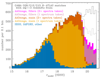
Figure 9: Histogram showing sources of redshifts to the H-ATLAS matched sample as a function of magnitude. The solid line shows the H-ATLAS-GAMA selected sample described in the text. The dotted line shows sources that either have a reliable redshift or were a GAMA target. The coloured filling is according to source of redshift.

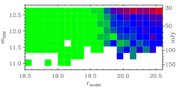
Figure 10: Redshift completeness of the H-ATLAS-GAMA sample as a function of 250-$\mu$m magnitude and $r_{\rm model}$. The colour scale representing completeness percentage is the same as in Fig. 4.

Targeting completeness is defined as the percentage of objects in a sample that have been observed spectroscopically. This is essentially 100% for targets that are in the main survey (15 453), but depends on $m_{250}$ for non-main survey targets (4 927) as shown in Fig. 11. From this, it is clear that the targeting completeness is high for $m_{250}<12.35\,\mathrm{mag}$ and drops off significantly at fainter magnitudes. This reflects the change in the cross-identifications between GAMA filler selection and the H-ATLAS data release (Bourne et al., 2016).

Figure 11: Targeting completeness for the H-ATLAS-GAMA sample as a function of $m_{250}$. The solid and dashed line show the completeness for non-main survey and main survey sources. The dotted line shows the fraction of the non-main survey sources that were assigned as filler targets in February 2011.

The other feature of the redshift completeness map shown in Fig. 10 is the drop off toward fainter $r_{\rm model}$. This is caused by a decrease in the redshift success rate, which is defined as the percentage of spectroscopically-observed targets that have a reliable redshift measurement, as shown in Fig. 12. To summarize, the redshift completeness map of the H-ATLAS-GAMA sample in Fig. 10 can be explained in terms of: 100% targeting completeness for main survey sources; about 75% targeting completeness for non-main survey sources at $m_{250}<12.35\,\mathrm{mag}$ with a drop off fainter than this; and for all sources, a general decrease in redshift success rate with $r_{\rm model}$ fainter than 19.5.

Figure 12: Redshift success rate as a function of $r_{\rm model}$ for the H-ATLAS-GAMA sample.

To show the demographics of the H-ATLAS-GAMA sample, we select sources with galaxy spectroscopic redshifts less than 0.8, $m_{250}<12.35\,\mathrm{mag}$, a random selection of 75% of the main survey, and all the fillers to $r_{\rm model}<20.6\,\mathrm{mag}$. This is unbiased within these magnitude limits other than the redshift success rate variation (Fig. 12). The distribution of this sample in visible-band absolute magnitude versus redshift is shown in Fig. 13, with colour coding according to far-IR luminosity. This clearly demonstrates the increase in the number density of the most luminous far-IR galaxies ($L_{250}>10^{25}{\rm W\,Hz}^{-1}$; cf. Dye et al. 2010; Guo et al. 2014). The filler sample is particularly useful for selecting luminous far-IR galaxies at $0.4<z<0.8$.

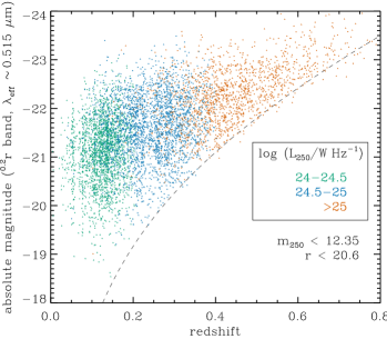
Figure 13: Demographics of the H-ATLAS-GAMA sample to $r_{\rm model}<20.6\,\mathrm{mag}$ and $m_{250}<12.35\,\mathrm{mag}$ with spectroscopic redshifts. The dashed line shows the $r$-band magnitude limit using an average k-correction as a function of redshift. The points are colour coded according to their 250-$\mu$m rest-frame luminosity, which is estimated using $m_{250}$ and an average k-correction as a function of redshift.

5 Data management units

The GAMA database is organised into data management units (DMUs). Here they are briefly introduced with any significant updates noted.

5.1 Spectroscopic, redshift and input catalogue DMUs

5.1.1 SpecCat

This DMU includes the spectra and redshifts obtained from the AAT, and tables combining the redshifts from all the curated spectroscopic data for the GAMA survey. In DR2, the redshifts from AAT spectra were obtained using the semi-automatic code runz (Saunders, Cannon, & Sutherland, 2004) with user interaction. For DR3, the primary choice of redshift has been updated; these are now from the automatic code autoz (Baldry et al., 2014) except for some broadlined-AGN spectra.

A detailed description of the redshift procedure using runz, and other spectroscopic survey procedures, are given in § 2 of Liske et al. (2015), while the autoz method and its calibration are described in detail in Baldry et al. (2014). An analysis of the survey redshift completeness, and a comparison between redshift accuracy from autoz and runz, are described in § 3 of Liske et al. (2015).

5.1.2 ExternalSpec

Spectra and redshifts were curated from 10 other surveys within the GAMA regions. These external spectroscopic surveys are used for 12% of the best redshifts of the main-survey targets (equatorial and G02 regions). This DMU is described in § 2.7 of Liske et al. (2015), and the list of surveys is given in table 2 of that paper.

5.1.3 EqInputCat

This DMU includes the input catalogue and the tiling catalogue for GAMA equatorial regions, G09, G12 and G15. The input catalogue was derived from SDSS. Previous versions of the tiling catalogue were used to track redshift completeness during the observations. The current version is designed to be used as a starting point for selecting well defined samples, from the best redshifts for each source and information on target selection. Visual classifications were made for a significant fraction of sources in order to identify deblends and artefacts.

A detailed description of the procedure for defining the input catalogue and selecting targets is given in Baldry et al. (2010). Updates to the DMU are described in § 2.9 of Driver et al. (2011) and § 2.1 of Liske et al. (2015).

5.1.4 G02InputCat

The input catalogue and tiling catalogue for the G02 region are described in § 2 and § 3 of this paper.

5.1.5 SpecLineSFR

This DMU contains three tables with line flux and equivalent width measurements for GAMA II spectra, which have $nQ>1$ and $0.002<z<1.35$. As well as providing the additional measurements for the G02 region, there are several key differences between this DMU version and an earlier version used in DR2 (Gunawardhana et al. 2013, Hopkins et al. 2013, § 5.1.10 of Liske et al. 2015). First, this DMU provides line fluxes and equivalent widths (EWs) measured in a consistent manner for spectra from several surveys that used AAOmega, SDSS, 2dF or 6dF; although we note that flux measurements are only useful for the SDSS and AAOmega spectra that were flux calibrated. Second, uncertainties are estimated for the line flux and EWs by propagating the formal uncertainties on the fitted parameters. Third, we include direct summation EW measurements for various line species, as well as estimates of the strength of the 4000Å  break, $D_{4000}$. Fourth, we include more complicated two-Gaussian fits to the $H\alpha$ and $H\beta$ emission lines where the second component accounts for broad emission or stellar absorption. We include various model selection techniques to determine where more complicated models are favoured over simple ones. The fitting, line measurements and model selection techniques are described in detail in Gordon et al. (2017).

5.1.6 LocalFlowCorrection

This DMU provides corrections from the heliocentric redshifts to the cosmic-microwave-background frame, and uses the flow model of Tonry et al. (2000) to provide redshifts primarily corrected for Virgo-cluster infall at low redshift. The procedure for, and the effect of, this are described in detail in § 2.3 of Baldry et al. (2012).

5.2 Image analysis DMUs

5.2.1 ApMatchedPhotom

This DMU provides AUTO (Kron) and Petrosian photometry, as well as other SExtractor outputs (Bertin & Arnouts, 1996) for the $ugrizZYJHK$ bands. The DMU is described in detail in Driver et al. (2016). This outlines the processing of the VISTA VIKING data (Sutherland, 2012; Edge et al., 2013) in detail, along with aperture-matched photometry from SDSS $ugriz$ and VISTA $ZYJHK$. As part of the process all data were smoothed to a common seeing FWHM of $2^{\prime\prime}$ to ensure accurate colour measurements. Earlier versions of ApMatchedPhotom were based on SDSS and UKIDSS (Warren et al., 2007)) data and later versions on SDSS and VISTA VIKING data where a significant improvement was seen in the near-IR colours in particular. ApMatchedPhotom has been superseded by the in-house lambdar code (Wright et al., 2016) but is included in this release for completeness and verification of earlier publications.

5.2.2 SersicPhotometry

The Sérsic Photometry DMU provides single-component Sersic (1968) fit results for sources across the GAMA equatorial survey regions. Independent fits are provided for each galaxy in each of the SDSS $ugriz$, UKIDSS $YJHK$ and VISTA $ZYJHK$ passbands. Galaxy models are constructed using sigma v1.0-2 (Structural Investigation of Galaxies via Model Analysis, Kelvin et al. 2012). sigma is a wrapper around several contemporary astronomy tools including Source Extractor (Bertin & Arnouts, 1996), PSF Extractor (Bertin, 2011) and GALFIT 3 (Peng et al., 2010), as well as analysis and processing code written in the open-source R programming language. In addition to standard GALFIT outputs, several additional value-added parameters are also output, such as truncated Sérsic magnitudes and central surface brightnesses. Further details on the fitting process and outputs may be found in Kelvin et al. (2012).

5.2.3 GalexPhotometry

This DMU contains catalogues for the NUV and FUV fluxes of each GAMA galaxy derived using three different methods. These are ‘simple match photometry’ (nearest neighbour), ‘advanced match photometry’ and ‘curve-of-growth (CoG) photometry’. In the second case, UV flux from the GALEX sources is distributed among the GAMA objects based on knowledge of the positions and sizes of the objects involved. In the CoG case, surface photometry is performed on the GALEX images at the optically-defined location of each GAMA galaxy, The procedures are extensively described in § 4.2 of Liske et al. (2015).

5.2.4 WISEPhotometry

This DMU provides the photometry from imaging with the Wide-field Infrared Survey Explorer for GAMA sources. The construction of the catalogue follows the methodology described in Cluver et al. (2014), in particular identifying and measuring resolved sources. Photometry of GAMA galaxies not resolved by WISE is taken from the AllWISE Catalogue; here the “standard aperture” photometry (w*mag) is used, and not the profile-fit photometry (w*mpro). This is to account for the sensitivity of WISE when observing extended, but unresolved sources (Driver et al., 2016). Further details can be found in Jarrett et al. (2017). All photometry in the DMU has been corrected to reflect the updated characterisation of the W4 filter as described in Brown, Jarrett, & Cluver (2014).

5.2.5 LambdarPhotometry

This DMU provides far-UV to far-IR aperture-matched photometry in 21-bands, measured consistently using the Lambda Adaptive Multi-Band Deblending Algorithm in R (lambdar; Wright et al. 2016). Photometry has been measured using apertures defined as described in Wright et al. (2016), where a considerable effort has been made to clean the input catalogue of apertures affected by contamination or extraction problems such as shredding. Additionally, the photometry is deblended from both GAMA sources and catalogued contaminants, which are defined independently for the far-UV to near-IR data, the mid-IR data, and the far-IR data. Fluxes from this DMU show considerable improvement in panchromatic consistency, i.e. smoothly changing behaviour with wavelength, when compared to the catalogue-matched photometry presented in Driver et al. (2016).

5.2.6 VisualMorphology

This catalogue provides a number of visual morphological classifications performed for various samples of galaxies in the equatorial survey regions. In total, 38 795 sources have one or more classifications.

• A basic visual classification using $giH$ images (SDSS and UKIDSS/VIKING) was made by 2 team members for sources with $0.002<z<0.1$. The classes used were: Elliptical, NotElliptical, Little Blue Spheroid (LBS), Star, Artefact and Uncertain. A earlier version of the classification was used in Driver et al. (2012).

• Hubble type galaxy classifications were made by 6 team members for sources with $0.002<z<0.06$. These were made using a decision tree, which was translated to the following classes: E, S0-Sa, SB0-SBa, Sab-Scd, SBab-SBcd, Sd-Irr, LBS, Star, Artefact. See § 3 of Kelvin et al. (2014) and § 3.1 of Moffett et al. (2016) for details.

• Disturbed galaxy classifications were made by 24 team members with multiple inspections of galaxies in close pairs and a control sample, over a redshift range of 0.01–0.33 depending on stellar mass. Inspections were made of inverted $grK$ images of 60 kpc $\times$ 60 kpc around each source using SDSS and VIKING data. The classes used were: Disturbed, Normal, and Unsure. See § 2.5 of Robotham et al. (2014) for details.

• A positional match was made to Galaxy Zoo 1 data (Lintott et al., 2011) for galaxies with $0.002<z<0.1$. The columns included in this DMU are: P_EL, P_CS, P_EL_DEBIASED, P_CS_DEBIASED. The first two give the raw fraction of Galaxy Zoo votes for Elliptical and NotElliptical, respectively, with the second two giving the values corrected for redshift bias. See Lintott et al. (2011) for details.

5.3 Spectral energy distribution DMUs

These DMUs make use of photometric measurements and redshifts to derive rest-frame luminosities, stellar population and dust properties.

5.3.1 kCorrections

K-corrections are provided in the GALEX FUV and NUV bands, the SDSS $ugriz$ bands and the UKIDSS $YJHK$ bands for all galaxies with redshifts in the GAMA equatorial survey regions (i.e. excluding G02). As well as the k-corrections themselves, we provide fourth-order polynomial fits to K($z$), the k-correction as a function of redshift, to aid in the calculation of Vmax values. These k-corrections are calculated using the eigentemplate fitting code kcorrect v4_2 of Blanton & Roweis (2007), and are further described in Loveday et al. (2012).

New for DR3, is that we provide k-corrections in passbands blueshifted by $z_{0}=0.2$ as well as 0.1 and 0.0. The advantage of using k-corrections for blueshifted passbands is that the uncertainties in the rest-frame magnitudes are smaller when the choice of bandpass shift is similar to the typical redshifts of a galaxy sample (cf. Fig. 13). We also provide k-corrections from fits to GAMA AUTO magnitudes (§ 5.2.1), in addition to those from SDSS model magnitudes. See § 2 of Loveday et al. (2015) for a discussion of the advantages of using GAMA AUTO magnitudes for this purpose.

5.3.2 StellarMasses

The StellarMasses DMU comprises estimates of total stellar mass and other population parameters (including mean stellar age, dust attenuation, etc.) based on stellar population synthesis (SPS) of the optical-to-near infrared SEDs. The fits are based on the Bruzual & Charlot (2003) simple stellar population models, assuming a Chabrier (2003) IMF, uniform metallicity, exponentially-declining star formation histories, and single-screen Calzetti et al. (2000) dust. The parameter estimation is done in a Bayesian way (rather than, for example, naive maximum likelihood), which has an important systematic effect on the inferred values for mass and mass-to-light ratio (M/L). The main reference for this DMU is Taylor et al. (2011).

The main improvement in the current version of this catalogue in comparison to DR2 is the incorporation of the VISTA-VIKING near-IR photometry, which largely removes the problems seen in Taylor et al. (2011) when using the UKIDSS near-IR data. In the fitting, the full $ugrizZYJHK$ SEDs are weighted in such a way that the fits are to a fixed restframe wavelength range of 3000–-11000 Å; i.e. restframe $u$-—$Y$. This decision is designed to protect against redshift-dependent biases arising from, for example, the different availabilities of restframe near-UV information for galaxies at different wavelengths. In practice, there are not significant redshift-dependent systematic differences between the current version of the StellarMasses DMU and earlier iterations.

Taylor et al. (2011) have shown that the numerical values of the SED-fit mass estimates can be approximated using the simple prescription (solar units): $\log(M_{*}/L_{i})=-0.68+0.70(g-i)_{\rm rest}$ with a typical 1-sigma uncertainty of $\sim 0.12$ dex. This provides authors with a simple way of deriving robust mass estimates from minimal information. Further, this provides a transparent way for authors to compare directly to the GAMA mass scale, in order to identify or account for possible systematic biases in the derivation of stellar mass estimates. Figure 14 (left) shows M/L versus observed $g-i$. There is still a tight correlation becoming less steep at higher redshift. Stellar mass derived using observed $g$ and $i$ magnitudes was used by Bryant et al. (2015) (their eq. 3) for a transparent stellar-mass selection avoiding the need for even SED-fit k-corrections.

Figure 14 (right) shows M/L in the $i$-band versus stellar mass for four redshift slices. This demonstrates the typical range in fitted M/L is from 0.2 to 2. At higher redshifts, GAMA samples becomes increasingly biased toward lower M/L because of the $r$-band magnitude selection limit. In order to create volume- and stellar-mass limited samples, one needs to select the unbiased region in M/L as demonstrated by the vertical lines in the figure. These limits were obtained using a method similar to Lange et al. (2015), see their fig. 1. Basically one needs to ensure that galaxies of every type (star-formation history, dust, profile), given a lower stellar-mass limit, could be selected over the redshift range of the sample. In practice, it is not always necessary to be quite so strict and one could relax the stellar-mass limits shown by $\sim 0.1$ dex.

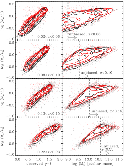
Figure 14: Mass-to-light ratios for four redshift slices versus observed colour (left) and stellar mass (right). Solar units are used for M/L and stellar mass. The red contours and points show stellar masses from the StellarMasses DMU (Taylor et al., 2011) while the black contours show the MagPhys DMU (Driver et al., 2017). The vertical dashed lines represent the lower limits in stellar mass for unbiased, volume-limited, samples for the four different redshift limits. Note the stellar masses use lambdar photometry whereas the samples are selected to $r_{\rm Petro}<19.8\,\mathrm{mag}$.

5.3.3 MagPhys

The MagPhys DMU is based on parsing the extinction-corrected flux and flux error for colours from lambdar through magphys (da Cunha et al., 2008). The code fits stellar and dust-emission templates to photometry, with dust attenuation applied to the stellar templates such that there is a balance between the attenuated and the dust-emitted energy. Energy balance is correct on average for a random distribution of galaxy inclinations, but will overestimate (underestimate) attenuation for face-on (edge-on) disks because of anisotropic attenuation. The MagPhys DMU provides estimates of a number of key parameters in particular the stellar mass, dust mass, and star-formation rate (SFR), which we consider reliable and useful for broader science. The DMU is described in detail in Driver et al. (2017).

This DMU provides stellar mass estimates in addition to the StellarMasses DMU (Taylor et al., 2011). Both use Bruzual & Charlot (2003) models for the stellar population synthesis and assume a Chabrier (2003) IMF. For the MagPhys DMU, the dust attenuation uses the Charlot & Fall (2000) model with absorption redistributed in wavelength assuming various dust components for dense stellar birth clouds and for the ambient inter-stellar medium (da Cunha et al., 2008). Fits are performed to the 21-band lambdar photometry using models with a range of exponentially-declining star-formation histories, with bursts, and a range of dust attenuation. Note however that that the key flux at 250 $\mu$m is only measured with a S/N $>2$ for about 30% of galaxies. Figure 14 (left) shows a comparison of the M/L, for the different stellar mass estimates, as a function of observed $g-i$. The median logarithmic offset varies from $-0.09$ for the lowest redshift slice, to $-0.03$ for the highest redshift slice shown. The good agreement between the stellar mass estimates demonstrates that the choice of dust attenuation approach does not make a significant difference.

The long-wavelength baseline (UV to far-IR) used by the MagPhys DMU also allow an estimate of SFR averaged over timescales less than a Gyr. MagPhys calculates SFRs from a combined UV and total IR SED fit, summing both the unobscured and obscured star formation, and provides various estimates over different timescales. For estimates of the SFR over the last 0.1 Gyr, the formal 1-sigma errors typically range from 0.2 dex to 0.6 dex. Detailed comparisons between these MagPhys SFRs and other SFR indicators in GAMA are discussed in Davies et al. (2016, 2017), and are used to determine the cosmic star-formation history in Driver et al. (2017).

5.4 Environment DMUs

5.4.1 GroupFinding

This DMU provides the GAMA Galaxy Group Catalogue (G3C) for the GAMA equatorial and G02 survey regions. The G3C is one of the major data products for the GAMA project. At the most basic level it is a friends-of-friends (FoF) group catalogue that has been run on GAMA survey style mocks to test the quality of the grouping and then run on the real GAMA data in order to extract our best effort groups. The details of the process are discussed extensively by Robotham et al. (2011).

There have been a number of minor changes since the first version used by the GAMA team. Redshifts now use the CMB frame instead of the heliocentric frame. We include galaxies with lower-quality $nQ=2$ redshifts (autoz calibrated probability of 0.4 to 0.9) because if these galaxies link with a group, they are likely at the correct redshift since the chance of accidentally being aligned with a group is small. The grouping parameters were re-calibrated over a larger suite of GAMA mock lightcones (Farrow et al., 2015) created using the Gonzalez-Perez et al. (2014) model.

The parameters are $b_{0}=0.0608$, $R_{0}=18.5000$, $E_{b}=0.0449$, $E_{r}=-0.0712$, and $\nu=0.7830$ as defined in § 2.1 of Robotham et al. (2011). These determine the linking length in the radial and line-of-sight directions as a function of survey location.

The impact of these new grouping parameters is ultimately very small, with grouping changes at the $\sim 1$% level. A bigger update has been to use the Farrow et al. (2015) randoms catalogue to determine the global redshift volume density [$n(z)$] rather than the luminosity function fit originally used in Robotham et al. (2011). Out to redshift $z=0.3$, the difference between the two methods for estimating the local density of observable points is small, but at higher redshifts they smoothly diverge at the 10% level, resulting in larger implied densities and smaller implied FoF links. The impact of this change is still fairly minor, but it does result in fewer grouped high-redshift galaxies.

5.4.2 FilamentFinding

Elements of large-scale structure are clearly visible in GAMA data. The FilamentFinding DMU identifies and characterizes filaments and voids using a multiple-pass modified minimum spanning tree (MST) algorithm. Initially, group centres from the GroupFinding DMU are used as nodes for a MST that identifies filaments. All galaxies within a distance $r$ of each filament are said to be filament galaxies associated with that structure. A second MST is generated from all galaxies that are not associated with filaments; this identifies smaller-scale interstitial structures dubbed as ‘tendrils’ (Alpaslan et al., 2014a), which typically contain few galaxies and exist within underdense regions. Galaxies that are beyond a distance $q$ from a tendril are said to be isolated void galaxies. $r$ and $q$ are selected so as to minimize the volume-weighted two point correlation function of the void galaxy population. For further details, see Alpaslan et al. (2014a, b).

5.4.3 GeometricEnvironments

This DMU identifies the cosmic web of large scale structure within the GAMA equatorial survey regions by classifying the geometric environment of each point in space as either a void, a sheet, a filament or a knot. The classification system is based on evaluation of the deformation tensor (i.e. the Hessian of the gravitational potential) on a grid. The number of eigenvalues above an imposed threshold indicates the number of collapsed dimensions of structure at that location – either 0, 1, 2 or 3, corresponding to a void, sheet, filament or knot, respectively. The classification of the grid, as given in the GeometricGrid table, allows the geometric environment of any object within the grid (any object in the G09, G12 or G15 regions with $0.04<z<0.263$) to be determined by assigning the object the same environment as the cell of the grid in which the object is located. See Eardley et al. (2015) for full details of the DMU.

5.4.4 EnvironmentMeasures

The EnvironmentMeasures DMU provides three different metrics of the local environment of GAMA galaxies. The three different metrics are the 5th nearest-neighbour surface density (Brough et al., 2013), the number of galaxies within a cylinder (Liske et al., 2015), and the adaptive Gaussian environment parameter (Yoon et al., 2008). The method used to calculate these has not changed from DR2 to DR3.

5.4.5 Randoms

The random catalogue DMU contains a series of randomly-placed points (‘randoms’), each tagged with a galaxy CATAID, that fill the volume of the equatorial fields of the GAMA survey in a way that follows the galaxy selection-function. It is designed to be used as a reference for measuring overdensities and estimating clustering statistics. See Farrow et al. (2015) for details.

The method used to produce these points was introduced in Cole (2011), whilst the particular implementation for GAMA is given in Farrow et al. (2015). The method involves cloning real galaxies, with each random point in the catalogue being stored with the CATAID of its parent. This allows the randoms to be assigned galaxy properties by matching on CATAID. Once properties are assigned to the randoms a suitable random catalogue can be produced by applying the same sample selection cuts as applied to the galaxies. One must, however, take care when using luminosity-selected samples, as a particular form of luminosity evolution is explicitly assumed in their production. In addition, if your sample has additional sources of incompleteness beyond the $r<19.8$ selection, for example a H${\alpha}$ flux limit, further work is required so please contact the DMU authors (for an example of this, see Gunawardhana et al. in preparation).

The DMU contains two tables. In RandomsUnwindowed the standard Cole (2011) method is used, whilst in the Randoms table the randoms created from a cloned galaxy are restricted to a window around the redshift of that galaxy, as explained in Farrow et al. (2015). The window is designed to minimise the impact of any unmodeled galaxy evolution effects on the random $n(z)$.

The DMU version of the randoms has two important differences to the ones used in Farrow et al. (2015). Firstly, the parameters used to model luminosity evolution have been changed following the results of Loveday et al. (2015). Secondly the size of the redshift window has been increased, to adjust the balance between limiting the effect of unmodeled galaxy-evolution and keeping the window large enough to completely remove large-scale structure from the input catalogue.

6 Data Release 3

The third GAMA data release (DR3) provides AAT/AAOmega spectra, redshifts and a wealth of ancillary information for primarily 215 260 objects from the GAMA II survey (Table 1). Of these, 178 856 are main survey objects and 36 404 are fillers. In turn, 150 465 (84%) and 4 344 (12%) of these, respectively, have secure redshifts. DR3 updates all data previously released in DR2, and significantly expands on DR2: DR3 includes both more objects and a wider range of data products than DR2. DR3 thus supersedes DR2 in every way. The data release is available at http://www.gama-survey.org/dr3/ .

In DR3 we are releasing data primarily for the following GAMA II objects:

• Main survey objects: all for G02 and G15, $r<19.0\,\mathrm{mag}$ selected for G09 and G12;

• Fillers: all for G02, H-ATLAS selected for G09, G12 and G15.

The region areas and main survey limits for GAMA I, GAMA II and DR3 are shown in Table 1. In addition, we include a small set of objects that were part of DR2 or the H-ATLAS DR1 and not already covered by the selection above. Note that for G02, we are releasing all GAMA II data, and for G15, all main survey data. The environment measurements that use the equatorial main survey are only available for G15.

GAMA DR3 doubles the number of galaxies with released spectroscopic redshifts compared to DR2 (Liske et al., 2015). New redshifts are available, in particular, for the G02 region (§ 3), H-ATLAS selected sources (§ 4), and in G15. The redshift measurements now use the more accurate autoz code (Baldry et al., 2014). New environment measurements for G15 are made available including a filament catalogue (Alpaslan et al., 2014a), and geometric measurements (Eardley et al., 2015). The galaxy distribution is shown in Fig. 15 with colour coding to showcase the different environment classifications. New image analysis is made available including lambdar photometry (Wright et al., 2016) that provides consistent photometry across all the bands from the far-UV to far-IR. All the available redshifts, including the G23 region, and all GAMA data products will be made available in DR4.

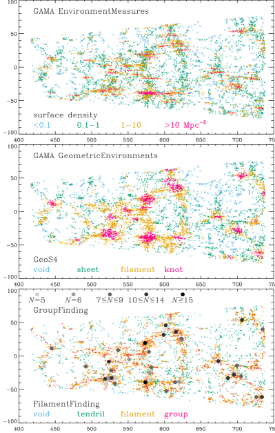
Figure 15: Galaxy distribution in the GAMA G15 field showing different environmental measurements. Galaxies were selected with $0.10<z<0.18$ and $-1.5\degr<\mathrm{dec}<1.5\degr$ (the two dimensions shown correspond to RA and redshift). Each panel shows the galaxies colour coded according to environment: top panel, using the 5th nearest neighbour surface density (Brough et al., 2013); middle panel, using the geometric environment classifications (Eardley et al., 2015); lower panel, using the filament-finder classifications (Alpaslan et al., 2014a). The top two panels show a volume-limited sample with $M_{r}<-20.0\,\mathrm{mag}$, while the filament finder uses only galaxies with $M_{r}<-20.55\,\mathrm{mag}$ ($h=0.7$). In the latter case, the classified groups, from the FoF catalogue (Robotham et al., 2011), used as the starting point of the filament finder, are those with two or more members from the volume-limited sample. Also shown are rich groups shaded according to the number of member galaxies with $M_{r}<-21.0\,\mathrm{mag}$ (cf. Fig. 7). Note also the FilamentFinding DMU provides links beween galaxies and groups in a filament.

References

- Aihara et al. (2011) Aihara H., et al., 2011, ApJS, 193, 29
- Alpaslan et al. (2014a) Alpaslan M. et al., 2014a, MNRAS, 438, 177
- Alpaslan et al. (2014b) Alpaslan M. et al., 2014b, MNRAS, 440, L106
- Baldry et al. (2014) Baldry I. K. et al., 2014, MNRAS, 441, 2440
- Baldry et al. (2012) Baldry I. K. et al., 2012, MNRAS, 421, 621
- Baldry et al. (2010) Baldry I. K. et al., 2010, MNRAS, 404, 86
- Bertin (2011) Bertin E., 2011, in ASP Conf. Ser. 442, Astronomical Data Analysis Software and Systems XX, Evans I. N., Accomazzi A., Mink D. J., Rots A. H., eds., ASP, San Francisco, p. 435
- Bertin & Arnouts (1996) Bertin E., Arnouts S., 1996, A&AS, 117, 393
- Blanton & Roweis (2007) Blanton M. R., Roweis S., 2007, AJ, 133, 734
- Boulade et al. (2003) Boulade O. et al., 2003, Proc. SPIE, 4841, 72
- Bourne et al. (2016) Bourne N. et al., 2016, MNRAS, 462, 1714
- Bremer et al. (2012) Bremer M. et al., 2012, Spitzer Proposal ID #90038
- Brough et al. (2013) Brough S. et al., 2013, MNRAS, 435, 2903
- Brown et al. (2014) Brown M. J. I., Jarrett T. H., Cluver M. E., 2014, Publ. Astron. Soc. Australia, 31, 49
- Bruzual & Charlot (2003) Bruzual G., Charlot S., 2003, MNRAS, 344, 1000
- Bryant et al. (2015) Bryant J. J. et al., 2015, MNRAS, 447, 2857
- Calzetti et al. (2000) Calzetti D., Armus L., Bohlin R. C., Kinney A. L., Koornneef J., Storchi-Bergmann T., 2000, ApJ, 533, 682
- Chabrier (2003) Chabrier G., 2003, PASP, 115, 763
- Charlot & Fall (2000) Charlot S., Fall S. M., 2000, ApJ, 539, 718
- Cluver et al. (2014) Cluver M. E. et al., 2014, ApJ, 782, 90
- Coil et al. (2011) Coil A. L. et al., 2011, ApJ, 741, 8
- Cole (2011) Cole S., 2011, MNRAS, 416, 739
- Colless et al. (2001) Colless M., et al., 2001, MNRAS, 328, 1039
- da Cunha et al. (2008) da Cunha E., Charlot S., Elbaz D., 2008, MNRAS, 388, 1595
- Dalton et al. (2006) Dalton G. B. et al., 2006, Proc. SPIE, 6269, 62690X
- Davies et al. (2016) Davies L. J. M. et al., 2016, MNRAS, 461, 458
- Davies et al. (2017) Davies L. J. M. et al., 2017, MNRAS, 466, 2312
- de Jong et al. (2013) de Jong J. T. A., Verdoes Kleijn G. A., Kuijken K. H., Valentijn E. A., 2013, Experimental Astronomy, 35, 25
- Dickinson & Giavalisco (2003) Dickinson M., Giavalisco M., 2003, in The Mass of Galaxies at Low and High Redshift, Bender R., Renzini A., eds., Springer-Verlag, p. 324
- Driver et al. (2017) Driver S. P. et al., 2017, MNRAS, in press (arXiv:1710.06628)
- Driver et al. (2011) Driver S. P. et al., 2011, MNRAS, 413, 971
- Driver et al. (2012) Driver S. P. et al., 2012, MNRAS, 427, 3244
- Driver et al. (2016) Driver S. P. et al., 2016, MNRAS, 455, 3911
- Driver et al. (2009) Driver S. P., et al., 2009, Astron. Geophys., 50, 5.12
- Dye et al. (2010) Dye S. et al., 2010, A&A, 518, L10
- Eales et al. (2010) Eales S. et al., 2010, PASP, 122, 499
- Eardley et al. (2015) Eardley E. et al., 2015, MNRAS, 448, 3665
- Edge et al. (2013) Edge A., Sutherland W., Kuijken K., Driver S., McMahon R., Eales S., Emerson J. P., 2013, The Messenger, 154, 32
- Erben et al. (2013) Erben T. et al., 2013, MNRAS, 433, 2545
- Farrow et al. (2015) Farrow D. J. et al., 2015, MNRAS, 454, 2120
- Garilli et al. (2014) Garilli B. et al., 2014, A&A, 562, A23
- Gonzalez-Perez et al. (2014) Gonzalez-Perez V., Lacey C. G., Baugh C. M., Lagos C. D. P., Helly J., Campbell D. J. R., Mitchell P. D., 2014, MNRAS, 439, 264
- Gordon et al. (2017) Gordon Y. A. et al., 2017, MNRAS, 465, 2671
- Gunawardhana et al. (2013) Gunawardhana M. L. P. et al., 2013, MNRAS, 433, 2764
- Guo et al. (2014) Guo Q. et al., 2014, MNRAS, 442, 2253
- Guo et al. (2013) Guo Q., White S., Angulo R. E., Henriques B., Lemson G., Boylan-Kolchin M., Thomas P., Short C., 2013, MNRAS, 428, 1351
- Gwyn (2012) Gwyn S. D. J., 2012, AJ, 143, 38
- Heymans et al. (2012) Heymans C. et al., 2012, MNRAS, 427, 146
- Hildebrandt et al. (2012) Hildebrandt H. et al., 2012, MNRAS, 421, 2355
- Hopkins et al. (2013) Hopkins A. M. et al., 2013, MNRAS, 430, 2047
- Jannuzi & Dey (1999) Jannuzi B. T., Dey A., 1999, in ASP Conf. Ser. 191, Photometric Redshifts and the Detection of High Redshift Galaxies, Weymann R., Storrie-Lombardi L., Sawicki M., Brunner R., eds., ASP, San Francisco, p. 111
- Jarrett et al. (2017) Jarrett T. H. et al., 2017, ApJ, 836, 182
- Jarvis et al. (2013) Jarvis M. J. et al., 2013, MNRAS, 428, 1281
- Kelvin et al. (2014) Kelvin L. S. et al., 2014, MNRAS, 439, 1245
- Kelvin et al. (2012) Kelvin L. S. et al., 2012, MNRAS, 421, 1007
- Kron (1980) Kron R. G., 1980, ApJS, 43, 305
- Kuijken et al. (2002) Kuijken K. et al., 2002, The Messenger, 110, 15
- Lacey et al. (2016) Lacey C. G. et al., 2016, MNRAS, 462, 3854
- Lange et al. (2015) Lange R. et al., 2015, MNRAS, 447, 2603
- Le Fèvre et al. (2013) Le Fèvre O. et al., 2013, A&A, 559, A14
- Lintott et al. (2011) Lintott C. et al., 2011, MNRAS, 410, 166
- Liske et al. (2015) Liske J. et al., 2015, MNRAS, 452, 2087
- Lonsdale et al. (2003) Lonsdale C. J. et al., 2003, PASP, 115, 897
- Loveday et al. (2015) Loveday J. et al., 2015, MNRAS, 451, 1540
- Loveday et al. (2012) Loveday J., et al., 2012, MNRAS, 420, 1239
- Moffett et al. (2016) Moffett A. J. et al., 2016, MNRAS, 457, 1308
- Oliver et al. (2012) Oliver S. J. et al., 2012, MNRAS, 424, 1614
- Pacaud et al. (2016) Pacaud F. et al., 2016, A&A, 592, A2
- Peng et al. (2010) Peng C. Y., Ho L. C., Impey C. D., Rix H.-W., 2010, AJ, 139, 2097
- Petrosian (1976) Petrosian V., 1976, ApJ, 209, L1
- Pierre et al. (2016) Pierre M. et al., 2016, A&A, 592, A1
- Robotham et al. (2010) Robotham A., et al., 2010, Publ. Astron. Soc. Australia, 27, 76
- Robotham et al. (2014) Robotham A. S. G. et al., 2014, MNRAS, 444, 3986
- Robotham et al. (2011) Robotham A. S. G. et al., 2011, MNRAS, 416, 2640
- Saunders et al. (2004) Saunders W., Cannon R., Sutherland W., 2004, Anglo-Australian Obser. Newsletter, 106, 16
- Schlegel et al. (1998) Schlegel D. J., Finkbeiner D. P., Davis M., 1998, ApJ, 500, 525
- Scoville et al. (2007) Scoville N. et al., 2007, ApJS, 172, 1
- Sersic (1968) Sersic J. L., 1968, Atlas de galaxias australes. Observatorio Astronomico, Universidad Nacional de Cordoba
- Sharp et al. (2006) Sharp R., et al., 2006, Proc. SPIE, 6269, 62690G
- Smith et al. (2011) Smith D. J. B. et al., 2011, MNRAS, 416, 857
- Stoughton et al. (2002) Stoughton C., et al., 2002, AJ, 123, 485
- Sutherland (2012) Sutherland W., 2012, in Science from the Next Generation Imaging and Spectroscopic Surveys, ESO, p. 40
- Taylor et al. (2011) Taylor E. N., et al., 2011, MNRAS, 418, 1587
- Tonry et al. (2000) Tonry J. L., Blakeslee J. P., Ajhar E. A., Dressler A., 2000, ApJ, 530, 625
- Valiante et al. (2016) Valiante E. et al., 2016, MNRAS, 462, 3146
- Warren et al. (2007) Warren S. J., et al., 2007, MNRAS, 375, 213
- Wright et al. (2016) Wright A. H. et al., 2016, MNRAS, 460, 765
- Yoon et al. (2008) Yoon J. H., Schawinski K., Sheen Y.-K., Ree C. H., Yi S. K., 2008, ApJS, 176, 414
- York et al. (2000) York D. G., et al., 2000, AJ, 120, 1579
- Ziparo et al. (2016) Ziparo F. et al., 2016, A&A, 592, A9