New method for the conformal bootstrap with OPE truncations

Abstract:

We investigate two aspects of conformal field theories. In the first part, we study the general 4-point correlator of identical scalars around the fully crossing symmetric point $u=v=1$, where $u,v$ are conformally invariant cross ratios. Since this point is fully crossing invariant, we can deduce some general properties of the 4-point correlators from crossing symmetry. In the second part, we discuss the conformal bootstrap with OPE truncations. As a generalization of Gliozzi’s method, we propose to extract the low-lying CFT data by minimizing the “error” induced by an OPE truncation. The error function $\eta$ measures the violation of crossing symmetry. The geometric interpretation of $\eta$ is the length of the vector associated with the truncated OPE. As an example, we apply the error-minimization method to the 2d Ising CFT with severely truncated OPEs.

1 Introduction

The conformal bootstrap program [1, 2, 3] attempts to solve conformal field theories using general principles, i.e. conformal symmetry and OPE associativity, where OPE stands for Operator Product Expansion. In 2d, the conformal symmetry algebra is infinite-dimensional, so many 2d CFTs are soluble. In higher dimensions, the conformal symmetry algebra is finite-dimensional and less powerful. However, since the original work [4], considerable progress in higher dimensional CFTs has been made using crossing symmetry [5]-[63]. A modern ingredient is the use of efficient numerical methods, such as semidefinite programming [32].

The bound method in [4] is based on a geometric interpretation of the crossing equation, where each conformal multiplet corresponds to a vector and the crossing equation is interpreted as the vanishing of the vector sum associated with the OPE. By searching for a separating plane for the potential vectors, one can detect the region where no unitary crossing solution can exist and rule out the non-unitary parameter space. The 3d Ising CFT happens to be located at a special point saturating the bound [13], which leads to precise determinations of the scaling dimensions of the low-lying operators.

However, a significant part of the CFT landscape remains unexplored. Many interesting CFTs from statistical mechanics are non-unitary and live outside the unitary domain. Even for unitary CFTs, it seems some information is not captured by the bounds. Complementary methods for the conformal bootstrap may be useful.

In general, a geometric vector is characterized by its direction and length. The bound method uses the information about the vector directions which are definite due to unitarity. Can we also make use of the information about the vector lengths? Many physical CFTs have a hierarchy in the magnitudes of OPE coefficients. The high-lying operators correspond to short vectors due to the suppression by small OPE coefficients.

In an effective field theory, it is typical that infinitely many terms are compatible with the assumed symmetry, but we can truncate the effective Lagrangian when the coupling constants of the subleading terms are comparably small. The effective description is consistent at the energy scales where the presumably leading terms are dominant. Analogously, in the context of conformal field theories, we should be able to truncate the operator product expansions if the subleading OPE coefficients are comparably small. These truncated OPEs will be referred to as “effective OPEs”. They characterize the effective descriptions of conformal field theories.

In [66], the effective conformal field theories were discussed in the context of the AdS/CFT correspondence [67, 68, 69]. In contrast to [66], we do not assume the CFTs under consideration are dual to certain gravitational theories in the bulk. Another important difference is that we emphasize the hierarchy in OPE coefficients, instead of operator dimensions [70]. These two hierarchies are related, but not equivalent. Operators of higher dimensions usually have smaller OPE coefficients, so a hierarchy in operator dimensions may correspond to a hierarchy in OPE coefficients. However, operators of low dimensions can decouple and then a hierarchy emerges in OPE coefficients, which is sometimes the defining property of physical CFTs.

In [71], Gliozzi proposed an alternative bootstrap method based on OPE truncations. In this approach, the operator product expansions are severely truncated and the low-lying spectra are captured by the zeros of certain truncation-related determinants. This method does not assume unitarity, so it can be applied to non-unitary CFTs [71]-[78]. For instance, the non-unitary Lee-Yang CFTs can be studied using this method.

Furthermore, based on a severe OPE truncation, a new type of universality for different CFTs in various dimensions was found using the inverse bootstrap method [79]. The low-lying CFT data are consistent with some universal relations when the effective OPEs of different CFTs share the same structure. This universality suggests effective OPE truncations should have board application.

In this work, we propose a new method for the conformal bootstrap with OPE truncations. The basic idea is to extract the low-lying CFT data by minimizing the “errors” induced by OPE truncations. We will introduce some error functions to quantify the discrepancies between crossing symmetry and OPE truncations. The error functions are constructed from truncated crossing equations. The non-trivial minimum of an error function can vanish, when the number of equations in the error function coincides with the number of free parameters in the truncated OPE. In this case, the error-minimization method is equivalent to Gliozzi’s determinant method. As a generalization of Gliozzi’s method, we consider error functions involving more equations. The nontrivial minima become strictly positive and the predictions are different from those of Gliozzi’s method. We expect to obtain more accurate results by increasing the number of equations in the error functions.

In [16], an analogous minimization procedure was introduced. After the scaling dimensions of low-lying operators were extracted from the extremal functional, the minimization procedure was performed to determine the OPE coefficients. In some sense, the new method proposed in this work also generalizes the minimization procedure in [16]. The difference is that we minimize the errors to extract both the spectral information and OPE coefficients. As a result, we do not need to assume unitarity which is crucial to the extremal functional method in [16].

Let us emphasize that our “errors” are not the standard errors that measure the accuracy of approximate CFT data. These error functions are devised to measure the violations of crossing symmetry due to OPE truncations, or the accuracy of the truncated crossing equations. The geometric interpretation of an error function is the vector length associated with a truncated OPE. The assumption behind the new method is that some physical OPEs converge rapidly and their truncated counterparts correspond to the minima of the error function.

Admittedly, it is not yet clear how to set the rigorous error bars, but we can examine the stability of the predictions by increasing the number of equations, which provides a criterion for selecting sensible results. Then we can estimate the errors in the predictions, based on the fact that crossing equations are only approximately solved.

The structure of this paper is as follows. In section 2, we discuss the general 4-point correlator of identical scalars and the conformal bootstrap around the fully crossing symmetric point $u=v=1$. In section 3, we present the method of error minimizations for the conformal bootstrap with OPE truncations. In section 4, we apply the error-minimization method to the 2d Ising CFT. In section 5, we summarize our results and discuss future directions.

2 Fully crossing symmetric point $u=v=1$

In this section, we will discuss the fully crossing symmetric point

$$u=v=1,$$ (2.1)

where the cross ratios $u,v$ are invariant under all crossing transformations. The conformal bootstrap around this crossing symmetric point has not been systematically investigated, in contrast to the standard one $u=v=1/4$. But this special point (2.1) has intrinsic value for the conformal bootstrap as it is fully crossing invariant. In section 2.1, we will study the general crossing solution expanded around $u=v=1$, which takes the form of a standard Taylor series. We will also discuss how to characterize the functional deviations of an interacting correlator from the correlator of generalized free fields.

In section 2.2, we will formulate the conformal bootstrap equations around $u=v=1$ and fix some notations to be used in section 3. When defining the error functions in section 3, we will treat equally the equations from different numbers of derivatives. Due to this naive construction, we will not consider the expansion around $u=v=1/4$. Instead, the equations from the expansion around $u=v=1$ are more appropriate. We will come back to this point in section 3. In addition, an advantage of expanding around $u=v=1$ is that we only need a small number of series coefficients of conformal blocks to achieve preliminary numerical precision. As a result, when the error-minimization method is explained in section 3, we will consider the conformal bootstrap around $u=v=1$. Note that it is not necessary to formulate the error-minimization method around this point.

2.1 General crossing solution

The conformally invariant cross ratios $u,v$ of 4-point correlators are defined as

$$u=\frac{x_{12}^{2}x_{34}^{2}}{x_{13}^{2}x_{24}^{2}},\quad v=\frac{x_{14}^{2}x_{23}^{2}}{x_{13}^{2}x_{24}^{2}},$$ (2.3)

where $x_{ij}=|x_{i}-x_{j}|$, and $x_{i}$ denotes the position of operator $\phi_{i}$. Under crossing transformations, they transform as

$$1\leftrightarrow 3 : \quad u\to v,\quad v\to u,$$ (2.4)

$$1\leftrightarrow 2 : \quad u\to u/v,\quad v\to 1/v,$$ (2.5)

$$1\leftrightarrow 4 : \quad u\to 1/u,\quad v\to v/u.$$ (2.6)

The line $u=v$ is invariant under the first crossing transformation (2.4), while the special point $u=v=1$ is invariant under all the crossing transformations (2.4), (2.5), (2.6). In terms of the variables $z,\,\bar{z}$, which are defined by $u=z\bar{z}$ and $v=(1-z)(1-\bar{z})$, the fully crossing symmetric point is at $z=1/2+i\sqrt{3}/2,\,\bar{z}=1/2-i\sqrt{3}/2$.

Let us consider the 4-point function of identical scalars,

$$<\phi(x_{1})\,\phi(x_{2})\,\phi(x_{3})\,\phi(x_{4})>=\frac{1}{(x_{12}^{2}x_{34}^{2})^{\Delta}}\,G(u,v),$$ (2.7)

where $\Delta$ is the scaling dimension of $\phi$.

Invariance under the first crossing transformation (2.4) implies

$$u^{-\Delta}G(u,v)=v^{-\Delta}G(v,u).$$ (2.8)

Let us introduce $H(u,v)=u^{-\Delta}G(u,v)$. From the first crossing equation (2.8), $H(u,v)$ is a symmetric function

$$H(u,v)=H(v,u).$$ (2.9)

The symmetric function $H(u,v)$ expanded around $u=v=1$ is a Taylor series of two variables

$$H(u,v)=\sum_{m,n=0}^{\infty}c_{m,n}(u-1)^{m}(v-1)^{n},\quad\text{with}\quad c_{m,n}=c_{n,m}.$$ (2.10)

Since $c_{m,n}$ is symmetric, let us consider $c_{m,n}$ with $m\geq n$ as the independent parameters. Under the second crossing transformation (2.5), invariance of the 4-point correlator indicates

$$G(u,v)=G(u/v,1/v).$$ (2.11)

The second crossing equation (2.11) imposes further constraints on the symmetric function $H(u,v)$

$$H(u,v)=u^{-\Delta}G(u/v,1/v)=v^{-\Delta}H(u/v,1/v),$$ (2.12)

which leads constraints on the series coefficients $c_{m,n}$. The third crossing transformation (2.6) does not lead to an independent equation.

The second crossing equation (2.12) can be solved order by order

$$H(u,v)=\sum_{k=0}^{\infty}H^{(k)}(u,v),$$ (2.13)

where $k$ indicates the order

$$H^{(k)}(u,v)=\sum_{m=0}^{k}c_{m,\,k-m}\,(u-1)^{m}(v-1)^{k-m}.$$ (2.14)

A few examples at low orders are:

• For $k=0$,

  $$H^{(0)}(u,v)=c_{0,0}\,,$$ (2.15)

  where $c_{0,0}$ is a free parameter. The arbitrariness of $c_{0,0}$ reflects the fact that $H(u,v)$ is crossing invariant at $u=v=1$.

• For $k=1$,

  $$H^{(1)}(u,v)=c_{1,0}(u-1)+c_{1,0}(v-1),$$ (2.16)

  where $c_{1,0}$ is related to $c_{0,0}$ as

  $$c_{1,0}=-\frac{1}{3}\Delta\,c_{0,0}.$$ (2.17)

  There is no independent parameter at this order.

• For $k=2$,

  $$H^{(2)}(u,v)=c_{2,0}(u-1)^{2}+c_{1,1}(u-1)(v-1)+c_{2,0}(v-1)^{2},$$ (2.18)

  where $c_{1,1}$ is a free parameter and $c_{2,0}$ is given by

  $$c_{2,0}=\frac{1}{3\times 2!}(\Delta)_{2}\,c_{0,0}-c_{1,1}\,.$$ (2.19)

  The notation $(x)_{n}$ is the Pochhammer symbol

  $$(x)_{n}=\Gamma(x+n)/\Gamma(x).$$ (2.20)

  One may consider $c_{2,0}$ as an arbitrary parameter and express $c_{1,1}$ in terms of $c_{0,0}$ and $c_{2,0}$. However, from the results at higher orders, it is more natural to consider the coefficients with $m\sim n$ as the independent parameters.

• For $k=3$,

  $$H^{(3)}(u,v)=\sum_{m=0}^{3}c_{m,\,3-m}\,(u-1)^{m}(v-1)^{3-m},$$ (2.21)

  where $c_{3,0}$ is not independent and we have

  $$c_{3,0}=-\frac{1}{3\times 3!}(\Delta)_{3}\,c_{0,0}+\frac{1}{3}(\Delta+2)\,c_{1,1}-\frac{2}{3}\,c_{2,1}\,.$$ (2.22)

  According to the comment in the $k=2$ case, we consider $c_{2,1}$ as the new independent parameter at this order.

It is straightforward to solve the second crossing equation (2.12) to higher orders. To the order $k=6$, $H(u,v)$ has 28 coefficients as a generic Taylor series. Using the first crossing equation (2.9), only 16 coefficients are independent. Then, from the second crossing equation (2.12), there remain 7 independent parameters: $c_{0,0}$, $c_{1,1}$, $c_{2,1}$, $c_{2,2}$, $c_{3,2}$, $c_{3,3}$, $c_{4,2}$. Note that we have two independent parameters at the order $k=6$.

We notice that $c_{0,0}$ appears only in $c_{n,0}$ and the coefficients of $c_{0,0}$ have a simple closed form expression

$$c_{n,0}=(-1)^{n}\frac{(\Delta)_{n}}{3n!}\,c_{0,\,0}+\dots,\quad n>0\,.$$ (2.23)

Let us consider the limit where the cross terms vanish. Then all the non-zero coefficients are proportional to $c_{0,0}$ and the complete crossing solution becomes

$$c_{0,0}+\sum_{n=1}^{\infty}(-1)^{n}\frac{(\Delta)_{n}}{3n!}\,c_{0,\,0}\left[(u-1)^{n}+(v-1)^{n}\right]=\frac{c_{0,0}}{3}\,(1+u^{-\Delta}+v^{-\Delta}),$$ (2.24)

which is a rescaled version of the 4-point function of the fundamental scalar in a generalized free theory. The normalization is fixed by $c_{0,0}$.

If the coefficients of the cross terms are small, the 4-point correlator around $u=v=1$ can be considered as a small deformation of the generalized free correlator. This then leads to the issue of how to characterize the deviation from the generalized free theory.

In a generic CFT, 2-point and 3-point correlators have the same functional forms as the generalized free ones due to conformal symmetry, but they can have different normalizations related to the OPE coefficients. In contrast, the functional form of a conformal 4-point correlator is not fully determined by conformal symmetry.

Since $u=v=1$ is invariant under all the crossing transformations, crossing symmetry is manifest around this fully crossing symmetric point. With this additional symmetry, we can deduce some general properties of the 4-point correlators. The zeroth order coefficient $c_{0,0}=H(1,1)$ corresponds to the normalization factor, which is analogous to 3-point function coefficients. The first order coefficients $c_{0,1},\,c_{1,0}$ are fixed by crossing symmetry, which means they coincide with those of the generalized free correlator, up to the normalization determined by $c_{0,0}$. In this sense, assuming $H(1,1)\neq 0$, all 4-point correlators are weakly interacting around the fully crossing symmetric point $u=v=1$.

Deviations from the generalized free theory start at the second order. In the generalized free correlator, there is no cross term, so the coefficient $c_{1,1}$ vanishes. We propose to use the ratio $R=c_{1,1}/c_{0,0}$ to characterize the leading deviation around $u=v=1$. By construction, this ratio $R$ vanishes in the generalized free theory. We can compute the exact values of $R$ in some 2d CFTs. In the 2d Ising CFT, the 4-point correlator of the spin correlator gives $R_{\text{2d Ising}}=-7/576\sim-0.012$. In the 2d Lee-Yang CFT, the 4-point correlator of the lowest scalar gives $R_{\text{2d LY}}\sim 0.025$. It is also natural to introduce higher order analogues $R_{m,n}=c_{m,n}/c_{0,0}$ using the other independent parameters.

The deviations from the generalized free theory was also discussed in [54], which was referred to as “non-Gaussianity”. Let us compare the measure of non-Gaussianity in [54] with our discussion above. In [54], the non-Gaussianity is measured by $Q$, the ratio of the interacting and generalized free correlators, as a function of the cross ratios. According to the criterion in [54], the spin correlators of the Ising CFTs in 2d and 3d show significant non-Gaussianity at $u=v=1$, because they correspond to the minima of $Q$ in the considered domain. This is different from our measure. Using a different ratio, we consider the functional deviations, which is generally weak around $u=v=1$. For instance, this is reflected by the plateau behavior of the Ising correlators shown in [54]. In addition, the reference point $z=0$ in [54] shows strong deviations from our functional perspective, which can be seen from the peak behavior . Nevertheless, the two ratios $Q,R$ are related, because $c_{1,1}=R\,H(1,1)$ measures the curvature of the $Q$-surface at $u=v=1$. From both perspectives, the Ising CFTs show significant departure from the generalized free theory in certain region of the Euclidean regime.

An interesting observation of the general crossing solution around $u=v=1$ is that the $\Delta$-dependence can be separated. To explain this observation, let us define $\bar{H}^{(k)}(u,v)$ as

$$H(u,v)=\sum_{k=0}^{\infty}(\Delta)_{k}\,\bar{H}^{(k)}(u,v),$$ (2.26)

with

$$\bar{H}^{(k)}(u,v)=\sum_{m=0}^{k}\bar{c}_{m,\,k-m}\,(u-1)^{m}(v-1)^{k-m}.$$ (2.27)

Then (2.17), (2.19), (2.22) become $\Delta$-independent equations:

$$\bar{c}_{1,0}=\frac{1}{3}\bar{c}_{0,0},\quad\bar{c}_{2,0}=\frac{1}{3\times 2!}\bar{c}_{0,0}-\bar{c}_{1,1},\quad\bar{c}_{3,0}=-\frac{1}{3\times 3!}\bar{c}_{0,0}+\frac{1}{3}\bar{c}_{1,1}-\frac{2}{3}\bar{c}_{2,1}.$$ (2.28)

The absence of $\Delta$ is verified by the explicit solutions of $\bar{c}_{m,n}$ to the order $k=6$. There may be more interesting results about the general structure of crossing solutions around $u=v=1$.

2.2 Conformal bootstrap

According to operator product expansion, the conformal invariant part of the 4-point function is decomposed into conformal blocks

$$G(u,v)=1+\sum_{i}P_{i}\,F_{\tau_{i},\,l_{i}}(u,v),$$ (2.29)

where $i$ labels the exchanged primary operators, $P_{i}$ are the squared OPE coefficients and $F_{\tau_{i},\,l_{i}}$ are the conformal blocks.

Crossing symmetry implies non-trivial equations for the CFT data. According to the conformal block expansion (2.29), the first crossing equation (2.8) expanded around $u=v=1$ gives

$$(\partial_{u}^{m}\partial_{v}^{n}-\partial_{u}^{n}\partial_{v}^{m})(u^{-\Delta})\Big{|}_{u=v=1}+\sum_{i}P_{i}\,(\partial_{u}^{m}\partial_{v}^{n}-\partial_{u}^{n}\partial_{v}^{m})\left[u^{-\Delta}F_{\tau_{i},\,l_{i}}(u,v)\right]\Big{|}_{u=v=1}=0.$$ (2.30)

The independent equations are

$$(-1)^{m}(\Delta)_{m}\,\delta_{n,0}+\sum_{i}P_{i}\,a_{m,n}(\Delta,\,\tau_{i},\,l_{i})=0,\quad m>n,$$ (2.31)

where $a_{m,n}$ are defined as

$$a_{m,n}(\Delta,\,\tau_{i},\,l_{i})=(\partial_{u}^{m}\partial_{v}^{n}-\partial_{u}^{n}\partial_{v}^{m})\left[u^{-\Delta}F_{\tau_{i},\,l_{i}}(u,v)\right]\Big{|}_{u=v=1}.$$ (2.32)

When a primary operator has even spins, the associated conformal block satisfies the second crossing equation (2.11). Therefore, the second crossing equation (2.11) is solved when all the exchanged primaries have even spins.

3 Minimizing the errors from OPE truncations

In this section, we will present a new method for the conformal bootstrap where operator product expansions are truncated. An operator product expansion is usually complicated, as the expansion leads to infinitely many operators in the sum. We will focus on the case where the OPE can be effectively truncated, which means the contributions from the high-lying operators are subleading. An effective OPE has finitely many parameters, so the bootstrap problem is more approachable. However, crossing symmetry is broken by the OPE truncation. We expect the crossing violation is weak when the low-lying CFT data are close to those of the effective OPEs. Therefore, we can extract the low-lying CFT data by minimizing the violation of crossing symmetry due to the OPE truncation. We will measure the crossing violation by some “error” functions, so the new method will be referred to as the error-minimization method.

The crossing equations (2.31) can be rewritten as

$$(-1)^{m}(\Delta)_{m}\,\delta_{n,0}+\sum_{i=1}^{N}P_{i}\,a_{m,n}(\Delta,\,\tau_{i},\,l_{i})=-\sum_{i>N}P_{i}\,a_{m,n}(\Delta,\,\tau_{i},\,l_{i}),$$ (3.33)

where $N$ is the number of exchanged primaries in the truncated OPE

$$\phi\times\phi=I+\sum_{i=1}^{N}P_{i}\,\mathcal{O}_{i},$$ (3.34)

and the right hand side of (3.33) is related to the high-lying operators omitted in the OPE truncation. Let us focus on the case $n=0$, so the first term on the left hand side of (3.33) is present and the convergence is usually rapid.

Before an exact solution is available, we do not know the exact content omitted in an OPE truncation, which are encoded in the right hand side of (3.33). However, according to (3.33), the error induced by the OPE truncation is equal to the left hand side of (3.33). Therefore, we should optimize the low-lying CFT data such that the left hand side of (3.33) is close to zero, which means the OPE-truncation error is minimized .

Let us define the “error” induced by an OPE truncation as

$$\eta(k)=\sqrt{\frac{1}{k}\sum_{m=1}^{k}\left[f_{m}(\Delta,\,\tau_{i},\,l_{i})\right]^{2}},$$ (3.35)

where $f_{m}$ are the truncated crossing equations, i.e. the left hand side of (3.33) with $n=0$,

$$f_{m}(\Delta,\,\tau_{i},\,l_{i})=(-1)^{m}(\Delta)_{m}+\sum_{i=1}^{N}P_{i}\,a_{m,0}(\Delta,\,\tau_{i},\,l_{i}),$$ (3.36)

and $k$ is the number of $f_{m}$ in the error function $\eta(k)$. These error functions measure the violations of crossing symmetry due to OPE truncations. We want to extract the physical CFT data by minimizing $\eta(k)$.

In (3.35), we use the equations from the expansion around $u=v=1$. Let us emphasize that the OPE convergence rate of a 4-point correlator at a point is different from that of its Taylor coefficients around the same point. Around $u=v=1/4$, the OPE convergence becomes less rapid when we increase the number of u- or v- derivatives. This is related to the fact that $u=v=1/4$ is on the boundary of the Euclidean regime. The equations from a large number of derivatives are probing the Lorentzian regime where the OPE convergence is slow. In contrast, for $u=v=1$, the OPE convergence is less sensitive to the number of derivatives, because this point is far from the Lorentzian regime. To make use of the rapid convergence around $u=v=1/4$, we need to introduce more sophisticated error functions, which will not be covered in this work.

The error function (3.35) has a geometric interpretation. We can think of the conformal block of a conformal multiplet $\{\mathcal{O}_{i},\,\partial^{k}\mathcal{O}_{i}\}$ as a vector

$$\vec{F}_{(i)}=\{a_{m,n}(\Delta,\,\tau_{i},\,l_{i})\},\quad m>n\geq 0,$$ (3.37)

whose components are labeled by two integers $m,n$. Then the exact crossing equation (2.31) indicates the infinite vector sum below gives the zero vector:

$$\vec{I}+\sum_{i=1}^{\infty}P_{i}\,\vec{F}_{(i)}=\vec{0},$$ (3.38)

where the identity operator is related to the vector $\vec{I}$ with

$$\vec{I}=\{(-1)^{m}(\Delta)_{m}\,\delta_{0,n}\},\quad m>n\geq 0.$$ (3.39)

To have the notion of length, let us introduce some inner products

$$<\vec{A},\,\vec{B}>_{(k)}\,=\frac{1}{k}\sum_{m=1}^{k}A_{m,0}\,B_{m,0}.$$ (3.40)

We can also define angles using the inner products. According to the definitions in (3.40), the error functions $\eta(k)$ coincide with the norms of the vector sum corresponding to the truncated OPE (3.34)

$$\eta(k)=\left\|\vec{I}+\sum_{i=1}^{N}P_{i}\,\vec{F}_{(i)}\right\|_{(k)}.$$ (3.41)

In general, we can reverse the procedure and define the error functions as the vector norms associated with the truncated OPEs. If the CFT data of the truncated OPE are exact, an error function also gives the norm of the vector sum corresponding to the high-lying operators

$$\eta(k)\Big{|}_{\text{exact}}=\left\|\sum_{i=N+1}^{\infty}P_{i}\,\vec{F}_{(i)}\right\|_{(k)},$$ (3.42)

where (3.38) is used.

Let us discuss the relation between Gliozzi’s determinant method [71] and our error-minimization method. When $k$ equals the number of free parameters in the truncated OPE, it is sometimes possible to minimize $\eta(k)$ to zero. If so, there exists a set of truncated CFT data which solve $k$ truncated crossing equations (3.36). We can interpret these equations as a system of linear equations, where the unknowns are the squared OPE coefficients $P_{i}$ and the coefficients of the unknowns are $a_{m,0}$ constructed from conformal blocks. To have a solution, at most $k_{P}$ equations are linearly independent. Note that $k_{P}$ is the number of unknown OPE coefficients and $k_{\tau}=k-k_{P}$ is the number of unknown twists. Let us imagine the constant part $(-1)^{m}(\Delta)_{m}+\dots$ is multiplied by an unknown whose solution is $P=1$, where $\dots$ indicates the terms with known OPE coefficients. Then we can construct $(k_{P}+1)$ by $(k_{P}+1)$ matrices from the coefficients of $(k_{P}+1)$ equations. Their determinants should vanish, otherwise the systems of $(k_{P}+1)$ homogeneous equations do not have any solution. In short, any set of $(k_{p}+1)$ equations should be linearly dependent. A solution with a vanishing “error” is precisely a crossing point of the hypersurfaces with vanishing determinants in Gliozzi’s method.

When the OPE convergence is rapid, the contributions of the high-lying operators are subleading, then the truncated crossing equations (3.36) from the same truncated OPE have weak linear independence. But they do not have exact linear dependence and the corresponding determinants should not vanish. As we increase $k$, the number of equations becomes greater than that of free parameters, then it is usually impossible to solve all the truncated equations (3.36) at the same time. The error function $\eta(k)$ becomes strictly positive. From (3.42), we expect the magnitude of the error function $\eta$ at the minimum is related to $P_{N+1}$

$$\eta\sim|P_{N+1}|,$$ (3.43)

where $P_{N+1}$ is the high-lying squared OPE coefficient with the largest absolute value. The precise coefficient in front of $|P_{N+1}|$ depends on the definition of $\eta$, the CFT under consideration , the truncation scheme and the normalization convention of the conformal blocks .

4 Example: the 2d Ising CFT

In this section, we will apply the error-minimization method to the 2d Ising CFT. We mainly consider a severely truncated OPE

$$\sigma\times\sigma=I+P_{\epsilon}\,\epsilon+P_{T}\,T,$$ (4.44)

where $\sigma$ is the spin operator, $I$ is the identity operator, $\epsilon$ is the energy operator, $T$ is the stress tensor, and $P_{\epsilon},\,P_{T}$ are the squared OPE coefficients of $\epsilon,T$.

Let us assume the scaling dimension $\Delta_{\sigma}$ of the spin operator $\sigma$ takes the exact value

$$\Delta_{\sigma}=1/8,$$ (4.45)

which is equal to the twist $\tau_{\sigma}$ because $\sigma$ is a scalar. Then we consider the error function $\eta(k)$ with various $k$ and extract the low-lying CFT data by minimizing $\eta(k)$. Note that $k$ is the number of truncated crossing equations (3.36) in $\eta(k)$. In Table 1, we summarize the predictions of the low-lying CFT data from the error-minimization method. We extract the results from the local minima in the domain of $\Delta_{\epsilon}>1/2$. We can see the approximate CFT data become more accurate as we increase $k$ and then stay around the exact values with errors of order $10^{-3}$. The minima of $\eta(k)$ with $k>3$ are of order $10^{-4}$, which are in accord with the magnitudes of the OPE coefficients of the leading high-lying operators, the level-4 Virasoro descendants. When $k>4$, the minimum of $\eta(k)$ is smaller for a larger $k$.

$k$	3	4	5	6	7	8	9	10	exact
$\Delta_{\epsilon}$	1.063	1.021	1.008	1.001	0.997	0.996	0.995	0.996	1
$P_{\epsilon}$	0.233	0.242	0.245	0.247	0.248	0.248	0.248	0.248	0.25
$P_{T}$	0.015	0.015	0.014	0.014	0.014	0.014	0.014	0.014	0.016

Table 1: The predictions from the error-minimization method of the low-lying CFT data of the 2d Ising CFT and the corresponding exact values. We use a severely truncated OPE $\sigma\times\sigma=I+P_{\epsilon}\,\epsilon+P_{T}\,T$ and assume $\Delta_{\sigma}=1/8$. $\Delta_{\sigma},\,\Delta_{\epsilon}$ are the scaling dimensions of the spin and energy operators. $P_{\epsilon},\,P_{T}$ are the squared OPE coefficients of the energy operator and the stress tensor. As we increase $k$, the predictions of $\Delta_{\epsilon},P_{\epsilon}$ become more accurate: the differences between the predictions and exact values are reduced by one order of magnitude.

Now we estimate the errors in the stable predictions. The predictions contain errors because the first crossing equation (2.8) is only approximately solved, which is related to the fact that $\eta(k)$ is non-zero. To set the error bars, let us examine the truncated crossing equations (3.36) one by one. When estimating the error in a CFT parameter, we consider this parameter as an unknown quantity and determine it from the truncated crossing equation $f_{m}=0$ using the other approximated CFT data. In this way, the OPE-truncation error in the crossing equation is all absorbed into this CFT parameter, so it will be different from the prediction of the error minimization. The result depends on which $f_{m}$ is used and the error bar will be set by the largest deviation from the error-minimized value.

In the case of $k=10$, the predictions from the error-minimization method read

$$k=10:\quad\Delta_{\epsilon}=0.9955(88),\quad P_{\epsilon}=0.2484(22),\quad P_{T}=0.0142(13),$$ (4.46)

which are compatible with the exact values

$$\Delta^{\text{exact}}_{\epsilon}=1,\quad P^{\text{exact}}_{\epsilon}=0.25,\quad P^{\text{exact}}_{T}=1/64\sim 0.0156.$$ (4.47)

The error in $P_{T}$ is slightly underestimated. As an example, let us explain in more detail how the error bar of $\Delta_{\epsilon}$ is determined. We solve $\Delta_{\epsilon}$ from $f_{m}=0$ with $m=1,2,\dots,10$, using $P_{\epsilon}=0.2484$ and $P_{T}=0.0142$. The results are around $\Delta_{\epsilon}=0.9955$, but with certain deviations. The largest deviation is from $f_{3}=0$, which gives $\Delta^{m=3}_{\epsilon}=1.0043$. The error bar is obtained from the difference $1.0043-0.9955=0.0088$.

Then we relax the assumption about the scaling dimension $\Delta_{\sigma}$ of the scalar operator $\sigma$. The spin and energy operators $\sigma,\,\epsilon$ are generalized to the Virasoro primaries $\phi_{1,2},\,\phi_{1,3}$ in the 2d CFTs. From the exact Virasoro OPE, we know the leading operators in the global OPE [15] are

$$\phi_{1,2}\times\phi_{1,2}=I+P_{1,3}\,\phi_{1,3}+P_{T}\,T+(P_{3}\,\phi_{3}+\dots),$$ (4.48)

where $\phi_{3}$ is a spin-2 primary with twist $\tau_{3}=\Delta_{1,3}$. The absolute value of $P_{T}$ is larger than that of $P_{3}$, so it is consistent to omit $\phi_{3}$ and use (4.44) as a crude approximation. In Figure 1, we present the predictions of $\Delta_{1,3}$ from error minimizations using the truncated OPE (4.44) with different $\Delta_{1,2}$. We notice that the $k$-dependence of the predictions is changed when $\Delta_{1,2}$ passes $1/8$, and the results are most stable at $\Delta_{1,2}=1/8$. We think these two phenomena are related to the behavior of $P_{3}$, the squared OPE coefficient of the subleading spin-2 operator $\phi_{3}$. From the exact solution, the signs of $P_{3}$ are different for $\Delta_{1,2}<1/8$ and $\Delta_{1,2}>1/8$, and $P_{3}$ vanishes at $\Delta_{1,2}=1/8$. It seems the change in $k$-dependence is related to the different signs of $P_{3}$. In addition, as $P_{3}=0$ at $\Delta_{1,2}=1/8$, the hierarchy in the OPE coefficients is larger. Therefore, the truncated OPE (4.44) becomes a better approximation around $\Delta_{1,2}=1/8$ and give more stable results.

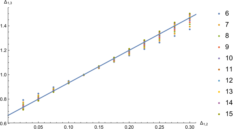
Figure 1: The exact relation (solid line) between $\Delta_{1,2}$ and $\Delta_{1,3}$, and the predictions (points) of $\Delta_{1,3}$ from the error-minimization method. We consider the truncated OPE: $\phi_{1,2}\times\phi_{1,2}=I+P_{1,3}\,\phi_{1,3}+P_{T}\,T$. We use the error function $\eta(k)$ with $k=6,7,\dots,15$. We choose $\Delta_{1,2}=0.025j$ with $j=1,2,\dots,12$. The predictions at $\Delta_{1,2}=0.125$ are very stable and match the exact value. The predictions become less accurate and less stable when $\Delta_{1,2}$ is far from $0.125$. When $\Delta_{1,2}<0.125$, the highest point corresponds to $k=6$ and the prediction decreases as we consider a larger $k$. When $\Delta_{1,2}>0.125$, the lowest point is associated with $k=6$ and the result increases as we choose a larger $k$.

In principle, we can determine $\Delta_{\sigma}$ according to the stability of the predictions from error minimizations. We compute the predictions of ${\Delta_{1,3}}$ from $k=5,6,\dots,15$ with $\Delta_{1,2}=0.12,\,0.125,\,0.13$. The standard deviation of $\Delta_{1,3}$ with $\Delta_{1,2}=0.125$ is smaller than the other two cases, so this crude comparison gives: $\Delta_{1,2}=0.125(5)$. However, when $\Delta_{1,2}$ is very close to $0.125$, $|P_{3}|$ decreases and $\phi_{3}$ is not the leading high-lying operator anymore. A precise determination of $\Delta_{\sigma}$ requires the introduction of other high-lying operators.

We can consider a longer truncated OPE. For example, we can take into account the level-4 Virasoro descendants, then the number of free parameters grows significantly. We need to consider much larger $k$’s in the error function $\eta(k)$, which requires more sophisticated numerical methods. We leave this investigation for the future.

Nevertheless, to test the error-minimization method, we can assume the spectral data are known and compute the OPE coefficients. In Table 2, we summarize the results for the truncated OPE

$$\sigma\times\sigma=I+P_{\epsilon}\,\epsilon+P_{T}\,T+P_{4}\,\phi_{4}+P_{5}\,\phi_{5}+P_{6}\,\phi_{6}\,,$$ (4.49)

with the spectral data

$$\Delta_{\sigma}=1/8,\,\Delta_{\epsilon}=1,\,\{\Delta_{4},\,l_{4}\}=\{4,\,0\},\,\{\tau_{5},\,l_{5}\}=\{0,\,4\},\,\{\tau_{6},\,l_{6}\}=\{1,\,4\}.$$ (4.50)

Since the spectral data are fixed, the predictions stabilize rapidly as we increase $k$. As expected, the predictions of $P_{\epsilon},\,P_{T}$ are more accurate than those from the shorter OPE (4.44): the differences between the predictions and exact results are decreased by one order of magnitude. The results of $P_{4},\,P_{5},\,P_{6}$ are not very accurate due to their small magnitudes, but the orders of magnitudes are consistent with the exact values. To improve the accuracy of $P_{4},\,P_{5},\,P_{6}$, we need to consider more subleading operators, such as the level-6 Virasoro descendants. The minima of $\eta(k)$ with $k>5$ are of order $10^{-6}$, which are consistent with the magnitudes of the leading high-lying OPE coefficients.

$k$	5	6	7	8	9	10	exact
$P_{\epsilon}$	0.2490	0.2492	0.2492	0.2492	0.2492	0.2491	0.25
$P_{T}$	0.0151	0.0152	0.0152	0.0152	0.0152	0.0152	0.0156
$P_{4}$	0.00018	0.00019	0.00019	0.00019	0.00019	0.00019	0.00024
$P_{5}$	0.00009	0.00011	0.00011	0.00011	0.00011	0.00011	0.00022
$P_{6}$	0.00004	0.00003	0.00003	0.00003	0.00003	0.00003	0.00002

Table 2: The predictions from the error-minimization method of the squared OPE coefficients of the 2d Ising CFT and the corresponding exact values with a few significant figures. We use the truncated OPE (4.49) and assume the spectral data take the exact values. The predictions are slightly improved as we increase $k$.

To obtain reasonable error bars of the predictions, we need to use more equations because the precision of the approximate crossing solutions is higher than the previous case (4.44). We will not discuss the error bars in this case.

5 Discussion

In this work, we study two aspects of conformal field theories:

The first part is about 4-point correlators around the fully crossing symmetric point $u=v=1$. Some general properties of the 4-point correlator of identical scalar operators are derived. We show that, around $u=v=1$, a generic 4-point correlator is close to the generalized free case. A new measure of deviations from the generalized free theory is proposed.

In the second part, we present a new method for the conformal bootstrap with OPE truncations, which generalizes Gliozzi’s method [71]. We propose to extract the low-lying CFT data by minimizing the OPE-truncation “errors”, i.e. the violations of crossing symmetry due to OPE truncations. Geometrically, these error functions are the lengths of the vectors corresponding to the truncated OPEs. The minimum of an error function also gives an estimate of the OPE coefficient of the leading high-lying operator omitted in the truncated OPE. We apply the error-minimization method to the 2d Ising CFT. We show the effectiveness of this new method and discuss how the predictions are influenced by the hierarchy in the OPE coefficients. Although the OPEs are severely truncated, the results of the 2d Ising CFT are fairly accurate and stable due to the decoupling of the subleading spin-2 primary operator. In addition, the error-minimization method can be used to extract OPE coefficients when the low-lying spectrum is known, for example in the extremal functional method [7, 16].

Let us discuss some possible directions for future research.

For the first part, we can generalize the results about the fully crossing symmetric point. 1) There are fully crossing-symmetric solutions with closed form expressions controlled by the other independent parameters. They deserve a more systematic investigation. 2) For the correlators of identical scalars, the second crossing equation is satisfied by each conformal block associated with a primary of even spins. However, for a generic correlator, the situation can be different and the general constraints from the second crossing equations may contain useful information. These two studies could lead to constructive results for the inverse conformal bootstrap [79].

For the second part, there are several interesting questions concerning the error-minimization method:

• By using efficient numerical techniques, we can study truncated OPEs with more operators. Then we have access to the refined structure of OPEs and can study more complex theories, such as 2d irrational CFTs and higher dimensional CFTs.

• We may improve the method by considering more sophisticated error functions. In (3.35), we use the equations from the Taylor expansion around a crossing symmetric point and assign the same weight to each equation. The way we choose equations and weights is not well justified. The equations from higher derivatives should be more sensitive to high-lying operators, so the predictions for a fixed truncated OPE could become unstable when $k$ in (3.35) is extremely large. The choice of weights is purely for simplicity. It seems more natural to consider the crossing equations evaluated at different points in the rapidly convergent regime [88, 48] and use them to define the error functions with appropriate weights. It will also be very interesting to implement the error-minimization method in an analytic manner.

• We want to know if rigorous bounds can be obtained using the triangle inequality in normed vector spaces, based on the small magnitudes of high-lying OPE coefficients. The role of vector lengths here will be in parallel to that of vector directions in the bound method based on unitarity.

6 Acknowledgements

I would like to thank Euihun Joung and Junchen Rong for stimulating discussions. I thank Slava Rychkov for constructive comments. I also want to thank Connor Behan for helpful correspondence. This work was supported by the National Research Foundation of Korea through the grant NRF-2014R1A6A3A04056670.

References

- [1] S. Ferrara, A. F. Grillo and R. Gatto, “Tensor representations of conformal algebra and conformally covariant operator product expansion,” Annals Phys. 76, 161 (1973). doi:10.1016/0003-4916(73)90446-6
- [2] A. M. Polyakov, “Nonhamiltonian approach to conformal quantum field theory,” Zh. Eksp. Teor. Fiz. 66, 23 (1974).
- [3] A. A. Belavin, A. M. Polyakov and A. B. Zamolodchikov, “Infinite Conformal Symmetry in Two-Dimensional Quantum Field Theory,” Nucl. Phys. B 241, 333 (1984). doi:10.1016/0550-3213(84)90052-X
- [4] R. Rattazzi, V. S. Rychkov, E. Tonni and A. Vichi, “Bounding scalar operator dimensions in 4D CFT,” JHEP 0812, 031 (2008) doi:10.1088/1126-6708/2008/12/031 [arXiv:0807.0004 [hep-th]].
- [5] V. S. Rychkov and A. Vichi, “Universal Constraints on Conformal Operator Dimensions,” Phys. Rev. D 80, 045006 (2009) doi:10.1103/PhysRevD.80.045006 [arXiv:0905.2211 [hep-th]].
- [6] F. Caracciolo and V. S. Rychkov, “Rigorous Limits on the Interaction Strength in Quantum Field Theory,” Phys. Rev. D 81, 085037 (2010) doi:10.1103/PhysRevD.81.085037 [arXiv:0912.2726 [hep-th]].
- [7] D. Poland and D. Simmons-Duffin, “Bounds on 4D Conformal and Superconformal Field Theories,” JHEP 1105, 017 (2011) doi:10.1007/JHEP05(2011)017 [arXiv:1009.2087 [hep-th]].
- [8] R. Rattazzi, S. Rychkov and A. Vichi, “Central Charge Bounds in 4D Conformal Field Theory,” Phys. Rev. D 83, 046011 (2011) doi:10.1103/PhysRevD.83.046011 [arXiv:1009.2725 [hep-th]].
- [9] R. Rattazzi, S. Rychkov and A. Vichi, “Bounds in 4D Conformal Field Theories with Global Symmetry,” J. Phys. A 44, 035402 (2011) doi:10.1088/1751-8113/44/3/035402 [arXiv:1009.5985 [hep-th]].
- [10] A. Vichi, “Improved bounds for CFT’s with global symmetries,” JHEP 1201, 162 (2012) doi:10.1007/JHEP01(2012)162 [arXiv:1106.4037 [hep-th]].
- [11] D. Poland, D. Simmons-Duffin and A. Vichi, “Carving Out the Space of 4D CFTs,” JHEP 1205, 110 (2012) doi:10.1007/JHEP05(2012)110 [arXiv:1109.5176 [hep-th]].
- [12] S. Rychkov, “Conformal Bootstrap in Three Dimensions?,” arXiv:1111.2115 [hep-th].
- [13] S. El-Showk, M. F. Paulos, D. Poland, S. Rychkov, D. Simmons-Duffin and A. Vichi, “Solving the 3D Ising Model with the Conformal Bootstrap,” Phys. Rev. D 86, 025022 (2012) doi:10.1103/PhysRevD.86.025022 [arXiv:1203.6064 [hep-th]].
- [14] M. Hogervorst, M. Paulos and A. Vichi, “The ABC (in any D) of Logarithmic CFT,” JHEP 1710, 201 (2017) doi:10.1007/JHEP10(2017)201 [arXiv:1605.03959 [hep-th]].
- [15] P. Liendo, L. Rastelli and B. C. van Rees, “The Bootstrap Program for Boundary ,” JHEP 1307, 113 (2013) doi:10.1007/JHEP07(2013)113 [arXiv:1210.4258 [hep-th]].
- [16] S. El-Showk and M. F. Paulos, “Bootstrapping Conformal Field Theories with the Extremal Functional Method,” Phys. Rev. Lett. 111, no. 24, 241601 (2013) doi:10.1103/PhysRevLett.111.241601 [arXiv:1211.2810 [hep-th]].
- [17] F. Kos, D. Poland and D. Simmons-Duffin, “Bootstrapping the vector models,” JHEP 1406, 091 (2014) doi:10.1007/JHEP06(2014)091 [arXiv:1307.6856 [hep-th]].
- [18] L. F. Alday and A. Bissi, “The superconformal bootstrap for structure constants,” JHEP 1409, 144 (2014) doi:10.1007/JHEP09(2014)144 [arXiv:1310.3757 [hep-th]].
- [19] D. Gaiotto, D. Mazac and M. F. Paulos, “Bootstrapping the 3d Ising twist defect,” JHEP 1403, 100 (2014) doi:10.1007/JHEP03(2014)100 [arXiv:1310.5078 [hep-th]].
- [20] M. Berkooz, R. Yacoby and A. Zait, “Bounds on superconformal theories with global symmetries,” JHEP 1408, 008 (2014) Erratum: [JHEP 1501, 132 (2015)] doi:10.1007/JHEP01(2015)132, 10.1007/JHEP08(2014)008 [arXiv:1402.6068 [hep-th]].
- [21] S. El-Showk, M. F. Paulos, D. Poland, S. Rychkov, D. Simmons-Duffin and A. Vichi, “Solving the 3d Ising Model with the Conformal Bootstrap II. c-Minimization and Precise Critical Exponents,” J. Stat. Phys. 157, 869 (2014) doi:10.1007/s10955-014-1042-7 [arXiv:1403.4545 [hep-th]].
- [22] Y. Nakayama and T. Ohtsuki, “Approaching the conformal window of symmetric Landau-Ginzburg models using the conformal bootstrap,” Phys. Rev. D 89, no. 12, 126009 (2014) doi:10.1103/PhysRevD.89.126009 [arXiv:1404.0489 [hep-th]].
- [23] Y. Nakayama and T. Ohtsuki, “Five dimensional -symmetric CFTs from conformal bootstrap,” Phys. Lett. B 734, 193 (2014) doi:10.1016/j.physletb.2014.05.058 [arXiv:1404.5201 [hep-th]].
- [24] S. M. Chester, J. Lee, S. S. Pufu and R. Yacoby, “The superconformal bootstrap in three dimensions,” JHEP 1409, 143 (2014) doi:10.1007/JHEP09(2014)143 [arXiv:1406.4814 [hep-th]].
- [25] F. Kos, D. Poland and D. Simmons-Duffin, “Bootstrapping Mixed Correlators in the 3D Ising Model,” JHEP 1411, 109 (2014) doi:10.1007/JHEP11(2014)109 [arXiv:1406.4858 [hep-th]].
- [26] F. Caracciolo, A. Castedo Echeverri, B. von Harling and M. Serone, “Bounds on OPE Coefficients in 4D Conformal Field Theories,” JHEP 1410, 020 (2014) doi:10.1007/JHEP10(2014)020 [arXiv:1406.7845 [hep-th]].
- [27] Y. Nakayama and T. Ohtsuki, “Bootstrapping phase transitions in QCD and frustrated spin systems,” Phys. Rev. D 91, no. 2, 021901 (2015) doi:10.1103/PhysRevD.91.021901 [arXiv:1407.6195 [hep-th]].
- [28] M. F. Paulos, “JuliBootS: a hands-on guide to the conformal bootstrap,” arXiv:1412.4127 [hep-th].
- [29] J. B. Bae and S. J. Rey, “Conformal Bootstrap Approach to O(N) Fixed Points in Five Dimensions,” arXiv:1412.6549 [hep-th].
- [30] C. Beem, M. Lemos, P. Liendo, L. Rastelli and B. C. van Rees, “The superconformal bootstrap,” JHEP 1603, 183 (2016) doi:10.1007/JHEP03(2016)183 [arXiv:1412.7541 [hep-th]].
- [31] S. M. Chester, S. S. Pufu and R. Yacoby, “Bootstrapping vector models in 4 6,” Phys. Rev. D 91, no. 8, 086014 (2015) doi:10.1103/PhysRevD.91.086014 [arXiv:1412.7746 [hep-th]].
- [32] D. Simmons-Duffin, “A Semidefinite Program Solver for the Conformal Bootstrap,” JHEP 1506, 174 (2015) doi:10.1007/JHEP06(2015)174 [arXiv:1502.02033 [hep-th]].
- [33] N. Bobev, S. El-Showk, D. Mazac and M. F. Paulos, “Bootstrapping SCFTs with Four Supercharges,” JHEP 1508, 142 (2015) doi:10.1007/JHEP08(2015)142 [arXiv:1503.02081 [hep-th]].
- [34] F. Kos, D. Poland, D. Simmons-Duffin and A. Vichi, “Bootstrapping the O(N) Archipelago,” JHEP 1511, 106 (2015) doi:10.1007/JHEP11(2015)106 [arXiv:1504.07997 [hep-th]].
- [35] S. M. Chester, S. Giombi, L. V. Iliesiu, I. R. Klebanov, S. S. Pufu and R. Yacoby, “Accidental Symmetries and the Conformal Bootstrap,” JHEP 1601, 110 (2016) doi:10.1007/JHEP01(2016)110 [arXiv:1507.04424 [hep-th]].
- [36] C. Beem, M. Lemos, L. Rastelli and B. C. van Rees, “The (2, 0) superconformal bootstrap,” Phys. Rev. D 93, no. 2, 025016 (2016) doi:10.1103/PhysRevD.93.025016 [arXiv:1507.05637 [hep-th]].
- [37] L. Iliesiu, F. Kos, D. Poland, S. S. Pufu, D. Simmons-Duffin and R. Yacoby, “Bootstrapping 3D Fermions,” JHEP 1603, 120 (2016) doi:10.1007/JHEP03(2016)120 [arXiv:1508.00012 [hep-th]].
- [38] D. Poland and A. Stergiou, “Exploring the Minimal 4D SCFT,” JHEP 1512, 121 (2015) doi:10.1007/JHEP12(2015)121 [arXiv:1509.06368 [hep-th]].
- [39] M. Lemos and P. Liendo, “Bootstrapping chiral correlators,” JHEP 1601, 025 (2016) doi:10.1007/JHEP01(2016)025 [arXiv:1510.03866 [hep-th]].
- [40] H. Kim, P. Kravchuk and H. Ooguri, “Reflections on Conformal Spectra,” JHEP 1604, 184 (2016) doi:10.1007/JHEP04(2016)184 [arXiv:1510.08772 [hep-th]].
- [41] Y. H. Lin, S. H. Shao, D. Simmons-Duffin, Y. Wang and X. Yin, “ = 4 superconformal bootstrap of the K3 CFT,” JHEP 1705, 126 (2017) doi:10.1007/JHEP05(2017)126 [arXiv:1511.04065 [hep-th]].
- [42] S. M. Chester, L. V. Iliesiu, S. S. Pufu and R. Yacoby, “Bootstrapping Vector Models with Four Supercharges in ,” JHEP 1605, 103 (2016) doi:10.1007/JHEP05(2016)103 [arXiv:1511.07552 [hep-th]].
- [43] S. M. Chester and S. S. Pufu, “Towards bootstrapping QED3,” JHEP 1608, 019 (2016) doi:10.1007/JHEP08(2016)019 [arXiv:1601.03476 [hep-th]].
- [44] F. Kos, D. Poland, D. Simmons-Duffin and A. Vichi, “Precision Islands in the Ising and Models,” JHEP 1608, 036 (2016) doi:10.1007/JHEP08(2016)036 [arXiv:1603.04436 [hep-th]].
- [45] Z. Komargodski and D. Simmons-Duffin, “The Random-Bond Ising Model in 2.01 and 3 Dimensions,” J. Phys. A 50, no. 15, 154001 (2017) doi:10.1088/1751-8121/aa6087 [arXiv:1603.04444 [hep-th]].
- [46] Y. Nakayama, “Bootstrap bound for conformal multi-flavor QCD on lattice,” JHEP 1607, 038 (2016) doi:10.1007/JHEP07(2016)038 [arXiv:1605.04052 [hep-th]].
- [47] S. El-Showk and M. F. Paulos, “Extremal bootstrapping: go with the flow,” arXiv:1605.08087 [hep-th].
- [48] A. Castedo Echeverri, B. von Harling and M. Serone, “The Effective Bootstrap,” JHEP 1609, 097 (2016) doi:10.1007/JHEP09(2016)097 [arXiv:1606.02771 [hep-th]].
- [49] Z. Li and N. Su, “Bootstrapping Mixed Correlators in the Five Dimensional Critical O(N) Models,” JHEP 1704, 098 (2017) doi:10.1007/JHEP04(2017)098 [arXiv:1607.07077 [hep-th]].
- [50] Y. Pang, J. Rong and N. Su, “ theory with F4 flavor symmetry in 6 ? 2 dimensions: 3-loop renormalization and conformal bootstrap,” JHEP 1612, 057 (2016) doi:10.1007/JHEP12(2016)057 [arXiv:1609.03007 [hep-th]].
- [51] Y. H. Lin, S. H. Shao, Y. Wang and X. Yin, “(2, 2) superconformal bootstrap in two dimensions,” JHEP 1705, 112 (2017) doi:10.1007/JHEP05(2017)112 [arXiv:1610.05371 [hep-th]].
- [52] M. Lemos, P. Liendo, C. Meneghelli and V. Mitev, “Bootstrapping superconformal theories,” JHEP 1704, 032 (2017) doi:10.1007/JHEP04(2017)032 [arXiv:1612.01536 [hep-th]].
- [53] C. Beem, L. Rastelli and B. C. van Rees, “More superconformal bootstrap,” arXiv:1612.02363 [hep-th].
- [54] S. Rychkov, D. Simmons-Duffin and B. Zan, ““Non-gaussianity of the critical 3d Ising model,” SciPost Phys. 2, no. 1, 001 (2017) doi:10.21468/SciPostPhys.2.1.001 [arXiv:1612.02436 [hep-th]].
- [55] D. Mazac, “Analytic Bounds and Emergence of Physics from the Conformal Bootstrap,” JHEP 1704, 146 (2017) doi:10.1007/JHEP04(2017)146 [arXiv:1611.10060 [hep-th]].
- [56] D. Simmons-Duffin, “The Lightcone Bootstrap and the Spectrum of the 3d Ising CFT,” JHEP 1703, 086 (2017) doi:10.1007/JHEP03(2017)086 [arXiv:1612.08471 [hep-th]].
- [57] S. Collier, P. Kravchuk, Y. H. Lin and X. Yin, “Bootstrapping the Spectral Function: On the Uniqueness of Liouville and the Universality of BTZ,” arXiv:1702.00423 [hep-th].
- [58] L. Iliesiu, F. Kos, D. Poland, S. S. Pufu and D. Simmons-Duffin, “Bootstrapping 3D Fermions with Global Symmetries,” arXiv:1705.03484 [hep-th].
- [59] A. Dymarsky, J. Penedones, E. Trevisani and A. Vichi, “Charting the space of 3D CFTs with a continuous global symmetry,” arXiv:1705.04278 [hep-th].
- [60] C. M. Chang and Y. H. Lin, “Carving Out the End of the World or (Superconformal Bootstrap in Six Dimensions),” arXiv:1705.05392 [hep-th].
- [61] Z. Li and N. Su, “3D CFT Archipelago from Single Correlator Bootstrap,” arXiv:1706.06960 [hep-th].
- [62] A. Dymarsky, F. Kos, P. Kravchuk, D. Poland and D. Simmons-Duffin, “The 3d Stress-Tensor Bootstrap,” arXiv:1708.05718 [hep-th].
- [63] N. B. Agmon, S. M. Chester and S. S. Pufu, “Solving M-theory with the Conformal Bootstrap,” arXiv:1711.07343 [hep-th].
- [64] M. A. Shifman, A. I. Vainshtein and V. I. Zakharov, “QCD and Resonance Physics. Theoretical Foundations,” Nucl. Phys. B 147, 385 (1979). doi:10.1016/0550-3213(79)90022-1
- [65] M. A. Shifman, A. I. Vainshtein and V. I. Zakharov, “QCD and Resonance Physics: Applications,” Nucl. Phys. B 147, 448 (1979). doi:10.1016/0550-3213(79)90023-3
- [66] A. L. Fitzpatrick, E. Katz, D. Poland and D. Simmons-Duffin, “Effective Conformal Theory and the Flat-Space Limit of AdS,” JHEP 1107, 023 (2011) doi:10.1007/JHEP07(2011)023 [arXiv:1007.2412 [hep-th]].
- [67] J. M. Maldacena, “The Large N limit of superconformal field theories and supergravity,” Int. J. Theor. Phys. 38, 1113 (1999) [Adv. Theor. Math. Phys. 2, 231 (1998)] doi:10.1023/A:1026654312961 [hep-th/9711200].
- [68] S. S. Gubser, I. R. Klebanov and A. M. Polyakov, “Gauge theory correlators from noncritical string theory,” Phys. Lett. B 428, 105 (1998) doi:10.1016/S0370-2693(98)00377-3 [hep-th/9802109].
- [69] E. Witten, “Anti-de Sitter space and holography,” Adv. Theor. Math. Phys. 2, 253 (1998) [hep-th/9802150].
- [70] I. Heemskerk, J. Penedones, J. Polchinski and J. Sully, “Holography from Conformal Field Theory,” JHEP 0910, 079 (2009) doi:10.1088/1126-6708/2009/10/079 [arXiv:0907.0151 [hep-th]].
- [71] F. Gliozzi, “More constraining conformal bootstrap,” Phys. Rev. Lett. 111, 161602 (2013) doi:10.1103/PhysRevLett.111.161602 [arXiv:1307.3111 [hep-th]].
- [72] F. Gliozzi and A. Rago, “Critical exponents of the 3d Ising and related models from Conformal Bootstrap,” JHEP 1410, 042 (2014) doi:10.1007/JHEP10(2014)042 [arXiv:1403.6003 [hep-th]].
- [73] F. Gliozzi, P. Liendo, M. Meineri and A. Rago, “Boundary and Interface CFTs from the Conformal Bootstrap,” JHEP 1505, 036 (2015) doi:10.1007/JHEP05(2015)036 [arXiv:1502.07217 [hep-th]].
- [74] Y. Nakayama, “Bootstrapping critical Ising model on three-dimensional real projective space,” Phys. Rev. Lett. 116, no. 14, 141602 (2016) doi:10.1103/PhysRevLett.116.141602 [arXiv:1601.06851 [hep-th]].
- [75] F. Gliozzi, “Truncatable bootstrap equations in algebraic form and critical surface exponents,” JHEP 1610, 037 (2016) doi:10.1007/JHEP10(2016)037 [arXiv:1605.04175 [hep-th]].
- [76] I. Esterlis, A. L. Fitzpatrick and D. Ramirez, “Closure of the Operator Product Expansion in the Non-Unitary Bootstrap,” JHEP 1611, 030 (2016) doi:10.1007/JHEP11(2016)030 [arXiv:1606.07458 [hep-th]].
- [77] S. Hikami, “Conformal Bootstrap Analysis for Yang-Lee Edge Singularity,” arXiv:1707.04813 [hep-th].
- [78] S. Hikami, “Conformal Bootstrap Analysis for Single and Branched Polymers,” arXiv:1708.03072 [hep-th].
- [79] W. Li, “Inverse Bootstrapping Conformal Field Theories,” arXiv:1706.04054 [hep-th].
- [80] D. Pappadopulo, S. Rychkov, J. Espin and R. Rattazzi, “OPE Convergence in Conformal Field Theory,” Phys. Rev. D 86, 105043 (2012) doi:10.1103/PhysRevD.86.105043 [arXiv:1208.6449 [hep-th]].
- [81] S. Rychkov and P. Yvernay, “Remarks on the Convergence Properties of the Conformal Block Expansion,” Phys. Lett. B 753, 682 (2016) doi:10.1016/j.physletb.2016.01.004 [arXiv:1510.08486 [hep-th]].
- [82] F. A. Dolan and H. Osborn, “Conformal four point functions and the operator product expansion,” Nucl. Phys. B 599, 459 (2001) doi:10.1016/S0550-3213(01)00013-X [hep-th/0011040].
- [83] F. A. Dolan and H. Osborn, “Conformal partial waves and the operator product expansion,” Nucl. Phys. B 678, 491 (2004) doi:10.1016/j.nuclphysb.2003.11.016 [hep-th/0309180].
- [84] C. Behan, “The unitary subsector of generalized minimal models,” arXiv:1712.06622 [hep-th].
- [85] S. Collier, Y. H. Lin and X. Yin, “Modular Bootstrap Revisited,” arXiv:1608.06241 [hep-th].
- [86] J. B. Bae, S. Lee and J. Song, “Modular Constraints on Conformal Field Theories with Currents,” arXiv:1708.08815 [hep-th].
- [87] E. Dyer, A. L. Fitzpatrick and Y. Xin, “Constraints on Flavored 2d CFT Partition Functions,” arXiv:1709.01533 [hep-th].
- [88] M. Hogervorst and S. Rychkov, “Radial Coordinates for Conformal Blocks,” Phys. Rev. D 87, 106004 (2013) doi:10.1103/PhysRevD.87.106004 [arXiv:1303.1111 [hep-th]].