Efficient and Invariant Convolutional Neural Networks for Dense Prediction

Abstract

Convolutional neural networks have shown great success on feature extraction from raw input data such as images. Although convolutional neural networks are invariant to translations on the inputs, they are not invariant to other transformations, including rotation and flip. Recent attempts have been made to incorporate more invariance in image recognition applications, but they are not applicable to dense prediction tasks, such as image segmentation. In this paper, we propose a set of methods based on kernel rotation and flip to enable rotation and flip invariance in convolutional neural networks. The kernel rotation can be achieved on kernels of 3 $\times$ 3, while kernel flip can be applied on kernels of any size. By rotating in eight or four angles, the convolutional layers could produce the corresponding number of feature maps based on eight or four different kernels. By using flip, the convolution layer can produce three feature maps. By combining produced feature maps using maxout, the resource requirement could be significantly reduced while still retain the invariance properties. Experimental results demonstrate that the proposed methods can achieve various invariance at reasonable resource requirements in terms of both memory and time.

I Introduction

With the development of high-performance hardware like GPU, deep learning has shown its great success in solving challenging problem in machine learning and artificial intelligence. Traditional machine learning techniques are usually based on handcrafted features, which would involve significant amount of engineering work and domain-specific prior knowledge. Deep learning techniques can automatically extract features from raw inputs and perform various tasks such as classification and segmentation [1].

Deep convolutional neural networks (CNNs) [2, 3] is a type of deep learning techniques that have achieved practical success on a variety of tasks, including image recognition [2, 3], segmentation [4], and reinforcement learning. One appealing property of CNNs is that they are invariant to translations on the inputs, making them particularly suitable for handling structured data like images and audio signals. However, such models are not invariant to other common transformations, such as rotation and flip. To cope with these problems, we usually use data augmentation to increase the number of training examples. Although this technique can achieve some level of invariance, it cannot guarantee rotation and flip invariance, since rotated copies of the same input usually lead to different outputs during prediction. Also, data augmentation is usually time-consuming as the training algorithm may take longer to reach convergence.

In order to address the above challenges, a few recent studies have attempted to construct CNNs that are invariant to generic transformations such as rotation and flip in image recognition applications [5]. These models achieve transformation invariance by generating and combining transformed copies of the same feature map. Due to their excessive resource requirement, these approaches are not readily applicable to dense prediction tasks, such as segmentation.

In this paper, we propose a set of techniques to construct efficient and invariant CNNs for dense prediction tasks [6]. The proposed solution includes rotating or flipping the kernels used in convolutional layers. It has been shown that rotating or flipping of kernels will have the same effect as rotating or flipping of feature maps [5]. By rotating and flipping the kernels in convolutional layer, the model will produce feature maps that can guarantee rotation and flip invariance. A key observation is that naïve implementation of many rotation and flip operations would lead to prohibitive memory requirement on segmentation problems. To address this challenge, we propose to use Maxout to reduce the resource requirement while still retain the invariance properties. Experimental results demonstrate that the proposed methods can achieve various invariance at reasonable resource requirements in terms of both memory and time. Note that, although the proposed methods are mainly described in the context of image segmentation in the following, the proposed methods are generically applicable to dense prediction tasks.

II Background and Related Work

Convolutional layers are not invariant to some image transformations such as flip and rotation. For a trained CNN, it may produce a different prediction if the input image is flipped. There are mainly two methods to improve the invariance of CNNs; those are, dealing with training examples, which is also called data augmentation, and incorporating image transformation invariance within the network.

II-A Data Augmentation

The key idea of data augmentation is to produce transformed training examples and feed them to the convolutional neural networks. By learning from these transformed images, the networks would also learn transformed features. The only work needed for data augmentation is to generate additional transformed training examples. Due to its simplicity, data augmentation has been widely used during the training process of various neural networks, such as AlexNet [3] and VGG net [7]. Simple data augmentation operations such as flip have even been integrated into many deep neural network tools. Although data augmentation is effective and easy to implement, it has several drawbacks. Specifically, data augmentation requires hand engineering on training examples and needs more training iterations for convergence. These additional costs reduce the efficiency of deep models during both training and testing.

II-B Invariant CNNs for Image Recognition

To overcome the limitation of data augmentation, some attempts have been made to incorporate transformation invariance into convolutional neural networks. Dieleman et al. [8] proposed to generate various rotated and flipped images and feed them into the same convolutional layer. The outputs of these layers are concatenated and fed to the following layers. This can deal with rotation and flip to some extent, but it still suffers from the tedious work of data augmentation. Dieleman et al. [9] proposed a framework that rotates feature maps within the network to achieve rotation invariance.

Cohen and Welling [5] studied rotation invariance and equivariance of convolutional neural networks from the perspective of group theory. They show that by operating on feature maps or kernels, the network can achieve invariance and equivariance. Both Dieleman et al. [9] and Cohen and Welling [5] show that rotating feature maps and rotating kernels within convolutional layers have the same effect.

III Efficient and Invariant CNNs for Dense Prediction

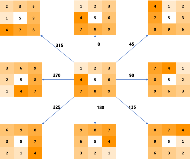
Figure 1: Illustration of how a $3\times 3$ convolutional kernel can be rotated by eight different angles to generate eight kernels.

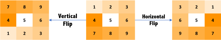
Figure 2: Illustration of how a $3\times 3$ convolutional kernel can be flipped horizontally and vertically.

III-A Dense Prediction

Dense prediction problems appear frequently in image-related applications like depth prediction [10], and image-to-image translation [11]. In this work, we focus on image semantic segmentation. Long et al. [4] proposed the fully convolutional network (FCN) for semantic segmentation. FCN employs a skip architecture to integrate semantic information from different layers, which helps to maintain low level features and spatial information for final dense prediction. Based on FCN, Ronneberger et al. [12] proposed the U-net, which uses symmetric encoder and decoder architecture. The encoder part encodes the input images into high-level feature maps by convolutional layers and max pooling layers. The decoder part restores it to segmentation maps of the same size as input image by up-convolution layers. In order to maintain low-level features and spatial information, skip connections are used in U-net. Another framework that deals with semantic segmentation is the deconvolution network proposed by Noh et al. [13]. This framework overcomes the limitations in FCN-based frameworks; namely fixed-size receptive field and over-simple deconvolution procedure. For common dense prediction tasks, data augmentation is also used to improve their performance.

III-B Kernel Rotation and Flip

In this paper, the rotation and flip invariance is achieved by rotating and flipping kernels. Although kernel rotation achieves the same effect as feature map rotation, it has various advantages. First, kernel operations would not require the feature maps to be in square shape. Second, kernel operations would be more flexible. For example, kernels could be rotated by various angles. In our new convolutional layers, kernels with size 3 $\times$ 3 could be rotated by 8 different angles: 0, 45, 90, 135, 180, 225, 270, and 315 degrees. Third, the number of parameters within the model would be reduced. For eight output feature maps in the new convolutional layers, they are produced by eight kernels with the same weights. The reduction of parameters could help to avoid the issue of over-fitting, especially for small training dataset.

In the new convolutional layer, kernel rotation is performed on 3 $\times$ 3 kernels. It has been shown that 3 $\times$ 3 kernels could achieve the effect of larger kernel sizes, such as 5 $\times$ 5 and 7 $\times$ 7, with even less parameters by stacking multiple convolutional layers. For VGG net, the kernel sizes of its convolutional layers are mostly 3 $\times$ 3. As 3 $\times$ 3 kernels could be rotated by eight angles, the kernel rotation could be implemented by at most 8 angles of 0, 45, 90, 135, 180, 225, 270 and 315 degrees. All eight rotated kernels will share the same set of parameters. For the new convolutional layer, kernels could be rotated by at most 8 different angles. The network could also choose to rotate kernels by 4 angles, which provides more flexibility for neural network construction. Trade-offs could be achieved between the number of rotated kernels and the number of output feature maps. In the experiment, the kernels in our convolutional layers are rotated by four angles: 0, 90, 180, 270 degrees. The number of output feature maps is doubled compared to the original convolutional layer. This will still save half of the parameters in the modified convolutional layers.

In the new convolutional layer, flip operations are also allowed. Kernels could be flipped both horizontally and vertically. This will produce three flipped versions of kernels within the new convolutional layer. Figure 2 shows how flip operations are implemented on kernels. Flipping kernel could be applied to kernels of any size. The number of output feature maps will only increase by three times when holding the number of parameters in the new convolutional layer the same as previous convolutional layer. In the experiment, the number of output feature maps for our new flip invariance convolutional layer increases to three times in order to maintain the same number of parameters.

III-C Efficient Invariance via Maxout

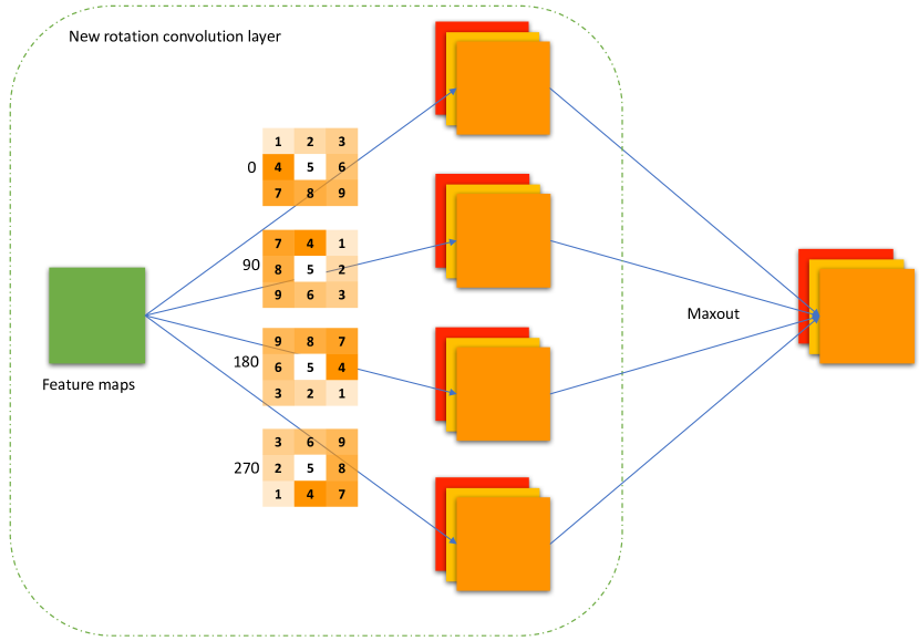
Figure 3: Illustration of how to combine rotation invariance convolutional layer and maxout to reduce the number of output feature maps.

In practice, the number of output feature maps of the new convolutional layer will be large in order to offset the effect of large reduction in the number of parameters in convolutional layers by parameter sharing. At the same time, the following convolutional layers would receive a large number of input feature maps. For these who want to use rotation and flip invariance convolutional layers, they may face the problem of memory requirement in the following convolution layers since the number of input feature maps increases significantly. In order to cope with this problem and also enable the flexibility of parameter numbers, we propose to use the maxout operation [14] in the new convolutional layer. The maxout networks, proposed by Goodfellow et al. [14], was designed to facilitate dropout and improve model performance. The key idea of maxout network is to output the max of several input feature maps. When applied to several feature maps with the same size, maxout will produce a single feature map of the same size. In this work, maxout is integrated with rotation and flip convolution layers to achieve rotation and flip invariance. Figures 3 and 4 show how maxout is integrated with rotation and flip invariant convolutional layers.

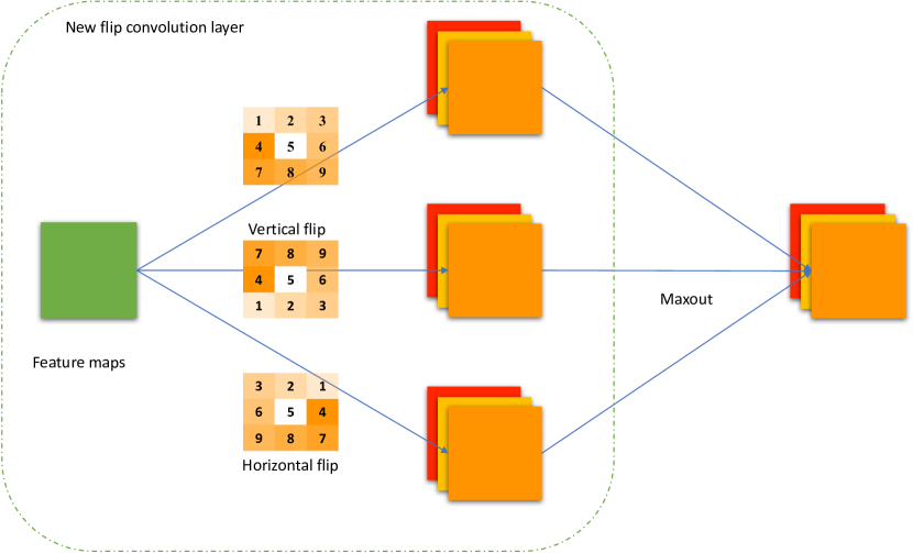
Figure 4: Illustration of how to combine flip invariance convolutional layer and maxout to reduce the number of output feature maps.

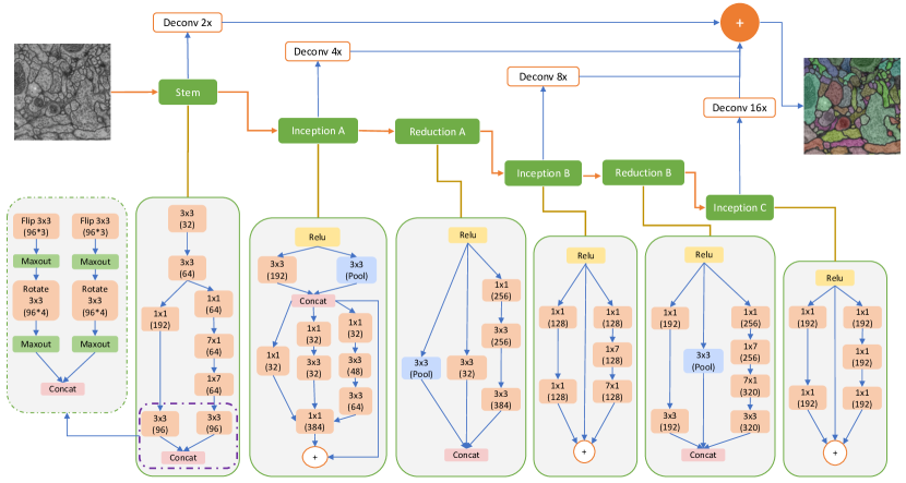
Figure 5: The convolutional neural network architecture used in this work. The two convolutional layers with 3 $\times$ 3 kernel size in the Stem part are replaced by the new convolutional layers to achieve rotation and flip invariance.

When flipping kernels within the new convolutional layers, the number of output feature maps will be tripled. The output feature maps can be divided into three parts corresponding to three kernels. The max operation will be performed on three feature maps. The output of maxout operation will produce the max value of these three set of feature maps. In this way, the number of input feature maps for the following layers remains the same. The same operation could be applied to rotation invariance convolutional layer. With the help of maxout operation, the new convolutional layers become more flexible when integrated into existing convolutional layers.

IV Experimental Studies

IV-A Dataset

We use the dataset from the open challenge on Circuit Reconstruction from Electron Microscopy Images (CREMI) to evaluate the proposed invariant CNNs. The CREMI dataset consists of brain electron microscopy images (EM), and the ultimate goal is to reconstruct neurons at the micro-scale level. A critical first step in neuron reconstruction is to segment the EM images. The main objective of neuron segmentation is to distinguish different neuron objects in the electron microscopy images. A common way for segmenting EM images is to predict the neuronal boundaries in the images [15]. For each pixel in the dense prediction output, there will be two labels with corresponding probabilities. Class 1 pixels correspond to boundaries in the image, and class 0 pixels correspond to all other structures. This task has an additional problem of imbalanced samples since there are far less boundary pixels in the image than non-boundary pixels. Thus, the commonly-used accuracy metric may not correctly reflect the performance of dense prediction models. In this situation, the ROC curve is used to evaluate models involved in this work, which could avoid the influence of imbalanced labels.

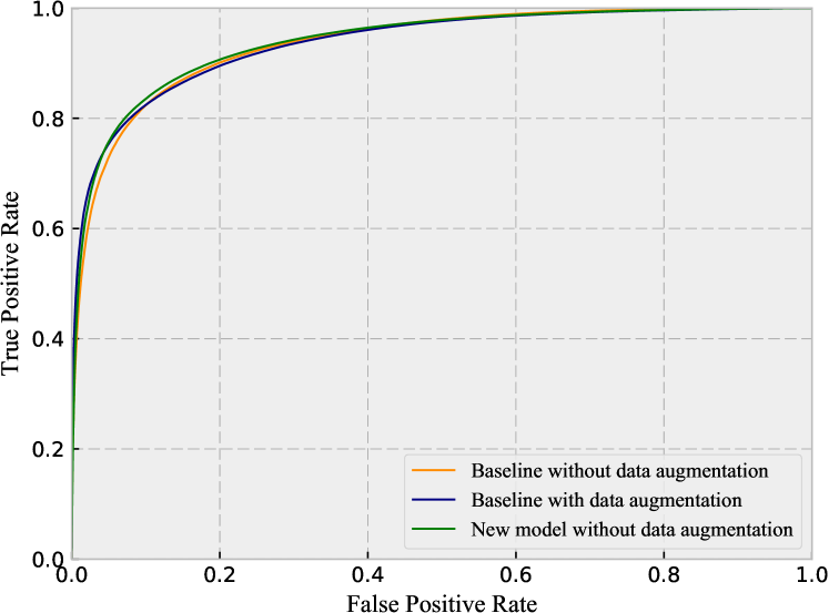
Figure 6: Comparison of the ROC curves of the three models.

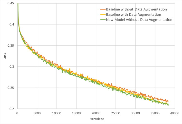
Figure 7: Comparison of the training losses of the three models at different iteration numbers.

IV-B Experimental Setup

The baseline CNNs model is given in Figure 5. The baseline model consists of six modules; namely Stem, Inception A, Reduction A, Inception B, Reduction B, and Inception C. The output feature maps from Stem, Inception A, and Inception B are processed by deconvolution and concatenated for final prediction. The six modules in the model are sequential, which means the latter modules will rely on the outputs of previous modules. As the modules in this model are sequential, we can replace several convolutional layers in the first module (Stem). If the rotation and flip invariance could be achieved in this module, it can be achieved in the following modules.

$\begin{array}[]{cccc}\includegraphics[width=203.80193pt]{FIG/outputsub1.pdf}&\includegraphics[width=203.80193pt]{FIG/outputsub2.pdf}&\includegraphics[width=203.80193pt]{FIG/outputsub3.pdf}&\includegraphics[width=203.80193pt]{FIG/outputsub4.pdf}\\ \mbox{Input image}&\mbox{Baseline without data augmentation}&\mbox{Baseline with data augmentation}&\mbox{New model without data augmentation}\end{array}$

Figure 8: Comparison of the results generated by the three models. The inputs are brain electron microscopy images, and the outputs are boundaries of neurons.

IV-C Deep Model Architectures

As in Figure 5, the two original convolutional layers in the Stem module are replaced by the new convolutional layers. By achieving rotation and flip invariance in these two convolutional layers, both the outputs of the Stem module and outputs of the following modules would be rotation and flip invariant. The kernel sizes of these two convolutional layers are both 3 $\times$ 3. The two original convolutional layers are replaced by two new convolutional layers; namely rotation invariant convolutional layer and flip invariant convolutional layer. In order to maintain the same performance of convolutional layers, the number of parameters in new convolutional layers are the same as before. The output features of flip invariant convolutional layer are tripled. The kernels in rotation invariant convolutional layer are rotated at angles of 0, 90, 180, and 270 degrees whose output features are quadrupled. To reduce the number of feature maps to the original number, two maxout layers are applied to ensure the use of the new invariant layers will have no influence on other parts of the model. The application of the new convolutional layers in this model would incur increased usage of memory, and the efficient invariance through maxout makes it affordable in most situations.

In this experiment, the baseline models with and without data augmentation are compared with the new model without data augmentation. For baseline model with data augmentation, the training images are augmented through a combination of rotation and flip operations. When making predictions, the input image will be processed with the same augmentation operations. The final prediction is based on majority voting of all dense prediction outputs. The model with data augmentation could also benefit from this ensemble strategy. However, since the prediction of the baseline model with data augmentation will produce more outputs, the total prediction time would be much longer than that of the baseline model without data augmentation. The model with the new convolutional layers does not need any data augmentations. The prediction process will be the same as the baseline model without data augmentation. It is anticipated that the prediction time of the new model will be slightly higher than that of the baseline model without data augmentation, since there are more layers and feature map outputs in the new convolutional layers. However, its prediction time would be much shorter than that of baseline model with data augmentation.

IV-D Flexibility on Rotation Angles

In this experiment, the kernels in the new rotation invariant convolutional layers are rotated by four angles: 0, 90, 180, and 270 degrees. In practice, the rotation angles could be more flexible. Usually, more rotation angles means more memory requirements. If memory resources are limited, the rotation angles could be reduced to 0 and 180. If better rotation invariant features are needed, the rotation angles could be increased to 0, 45, 90, 135, 180, 225, 270, and 315 degrees. The combination of maxout with the new convolutional layers could ensure that the number of final output feature maps is the same as the original layers. When using the new convolutional layers, there is great flexibility on rotation angles based on practical needs.

IV-E Analysis of Results

The dense prediction outputs of three models are given in Figure 8. Figure 7 shows the training loss of the three models at different iterations. The training loss of the baseline model without data augmentation is the highest among the three models. The new model without data augmentation even has the lowest training loss along the whole training iterations. This means the property of rotation and flip invariance in the new model help improve the training, since it could deal with features with arbitrary rotation and flip transformations. The baseline model without data augmentation does not have this invariance capability. The baseline model with data augmentation may be trained to learn this property but with much more iterations. From these results, it is clear that the baseline model with data augmentation has larger loss than the new model until after 35,000 iterations. But the loss of the baseline model without data augmentation is always higher than that of the new model. The gap between the loss curves of the baseline model without data augmentation and the new model even increases as iteration number increases.

Table I shows the model evaluation results using AUC values. Since the prediction output labels are imbalance, AUC values would be more meaningful in the evaluation. The AUC values of the new model and baseline model with data augmentation are similar and higher than that of the baseline model without data augmentation. This shows that the new model has very similar performance compared to the baseline model with data augmentation. This also demonstrates that data augmentation usually leads to improved performance, a results that is consistent with prior observations [16]. Figure 6 gives the ROC curves of three models.

Table II provides the prediction time for the three models. The baseline model without data augmentation has the highest prediction speed. The prediction time for the new model without data augmentation is slower than that of the baseline model without data augmentation. This is because there are more convolutional layers and more output feature maps in the new convolutional layers. As the replaced part is at the early stage of the model, the size of feature maps is relatively large, which could increase the computational time. The baseline model with data augmentation has the highest prediction time. It is far longer than that of the new model. The prediction process of the baseline model with data augmentation will produce eight dense prediction outputs corresponding to eight data augmentation operations in the training process. Thus, the total prediction time of the baseline model with data augmentation is eight times of that of the baseline model without data augmentation. Under the same prediction performance, less prediction time should be appreciated, which makes it more applicable in practice. Overall, the experimental results show that the proposed invariant methods achieve higher performance as compared to the original method without data augmentation. In addition, the proposed methods are very efficient when making predictions, as compared to the original methods with data augmentation.

TABLE I: Comparison of AUC values achieved by the three models.

Model	AUC values
Baseline without Data Augmentation	0.931
Baseline with Data Augmentation	0.939
New Model without Data Augmentation	0.941

V Conclusion and Discussion

In this work, we proposed a new convolutional layer that could achieve rotation and flip invariance. The new convolutional layer is implemented through kernel operations instead of feature map operations to make it more flexible and efficient. For rotation invariant convolutional layer, the kernels in the layer could be rotated at 8 angles: 0, 45, 90, 135, 180, 225, 270, and 315 degrees. The rotated angles could be reduced to 2 or 4 angles to meet memory constraints. For flip invariant convolutional layer, the original kernels are flipped both horizontally and vertically. In order to reduce the influence of increased number of feature maps from the new convolutional layers, we propose to use maxout to compress the feature maps. The combination of the new convolutional layers and maxout layer makes it even more flexible when applied to other models. In experiment, we compared the proposed new model with baseline models with and without data augmentation. The experimental results show that the proposed invariant methods achieve higher performance compared to the original method without data augmentation.

TABLE II: Comparison of the prediction time of the three models.

Model	Prediction Time
Baseline without Data Augmentation	28m
Baseline with Data Augmentation	226m
New Model without Data Augmentation	45m

References

- [1] I. Goodfellow, Y. Bengio, and A. Courville, Deep Learning. The MIT Press, 2016.
- [2] Y. LeCun, L. Bottou, Y. Bengio, and P. Haffner, “Gradient-based learning applied to document recognition,” Proceedings of the IEEE, vol. 86, no. 11, pp. 2278–2324, November 1998.
- [3] A. Krizhevsky, I. Sutskever, and G. E. Hinton, “Imagenet classification with deep convolutional neural networks,” in Advances in neural information processing systems, 2012, pp. 1097–1105.
- [4] J. Long, E. Shelhamer, and T. Darrell, “Fully convolutional networks for semantic segmentation,” in Proceedings of the IEEE Conference on Computer Vision and Pattern Recognition, 2015, pp. 3431–3440.
- [5] T. Cohen and M. Welling, “Group equivariant convolutional networks,” in Proceedings of The 33rd International Conference on Machine Learning, 2016, pp. 2990–2999.
- [6] M. A. Islam, N. Bruce, and Y. Wang, “Dense image labeling using deep convolutional neural networks,” in Computer and Robot Vision (CRV), 2016 13th Conference on. IEEE, 2016, pp. 16–23.
- [7] K. Simonyan and A. Zisserman, “Very deep convolutional networks for large-scale image recognition,” Proceedings of the International Conference on Learning Representations, 2015.
- [8] S. Dieleman, K. W. Willett, and J. Dambre, “Rotation-invariant convolutional neural networks for galaxy morphology prediction.” Monthly notices of the royal astronomical society., vol. 450, no. 2, pp. 1441–1459, 2015.
- [9] S. Dieleman, J. D. Fauw, and K. Kavukcuoglu, “Exploiting cyclic symmetry in convolutional neural networks,” in Proceedings of The 33rd International Conference on Machine Learning, 2016, pp. 1889–1898.
- [10] D. Eigen, C. Puhrsch, and R. Fergus, “Depth map prediction from a single image using a multi-scale deep network,” in Advances in neural information processing systems, 2014, pp. 2366–2374.
- [11] I. Laina, C. Rupprecht, V. Belagiannis, F. Tombari, and N. Navab, “Deeper depth prediction with fully convolutional residual networks,” in 2016 Fourth International Conference on 3D Vision. IEEE, 2016, pp. 239–248.
- [12] O. Ronneberger, P. Fischer, and T. Brox, “U-net: Convolutional networks for biomedical image segmentation.” in International Conference on Medical Image Computing and Computer-Assisted Intervention, 2015, pp. 234–241.
- [13] H. Noh, S. Hong, and B. Han, “Learning deconvolution network for semantic segmentation.” in IEEE International Conference on Computer Vision, 2015.
- [14] I. Goodfellow, D. Warde-farley, M. Mirza, A. Courville, and Y. Bengio, “Maxout networks,” in Proceedings of the 30th International Conference on Machine Learning (ICML-13), 2013, pp. 1319–1327.
- [15] A. Fakhry, T. Zeng, and S. Ji, “Residual deconvolutional networks for brain electron microscopy image segmentation,” IEEE Transactions on Medical Imaging, 2016.
- [16] A. Fakhry, H. Peng, and S. Ji, “Deep models for brain EM image segmentation: novel insights and improved performance,” Bioinformatics, vol. 32, pp. 2352–2358, 2016.