Evolutions of unequal mass, highly spinning black hole binaries

Abstract

We evolve a binary black hole system bearing a mass ratio of $q=m_{1}/m_{2}=2/3$ and individual spins of $S^{z}_{1}/m_{1}^{2}=0.95$ and $S^{z}_{2}/m_{2}^{2}=-0.95$ in a configuration where the large black hole has its spin antialigned with the orbital angular momentum, $L^{z}$, and the small black hole has its spin aligned with $L^{z}$. This configuration was chosen to measure the maximum recoil of the remnant black hole for nonprecessing binaries. We find that the remnant black hole recoils at $500km/s$, the largest recorded value from numerical simulations for aligned spin configurations. The remnant mass, spin, and gravitational waveform peak luminosity and frequency also provide a valuable point in parameter space for source modeling.

I Introduction

Since the breakthroughs in numerical relativity of 2005 Pretorius (2005); Campanelli et al. (2006a); Baker et al. (2006) it is possible to accurately simulate moderate-mass-ratio and moderate-spin black-hole binaries. State of the art numerical relativity codes now routinely evolve binaries with mass ratios as small as $q\lesssim 1/16$ Gonzalez et al. (2009); Lousto et al. (2010); Lousto and Zlochower (2011); Sperhake et al. (2011); Chu et al. (2016); Jani et al. (2016), and are pushing towards much smaller mass ratios. Indeed, there have been some initial explorations of $q=1/100$ binaries Lousto and Zlochower (2011); Sperhake et al. (2011).

However, when it comes to highly-spinning binaries, prior to the work of Lovelace et al. (2008) of the SXS Collaboration , it was not even possible to construct initial data for binaries with spins larger than $\sim 0.93$ Cook and York (1990). This limitation was due to the use of conformally flat initial data. Conformal flatness is a convenient assumption because the Einstein constraint system takes on a particularly simple form. Indeed, using the puncture approach, the momentum constraints can be solved exactly using the Bowen-York ansatz Bowen and York (1980). There were several attempts to increase the spins of the black holes while still preserving conformal flatness Dain et al. (2002); Lousto et al. (2012), but these introduced negligible improvements. Lovelace et al. Lovelace et al. (2008) were able to overcome these limitations by choosing the initial data to be a superposition of conformally Kerr black holes in the Kerr-Schild gauge. Using these new data, they were able to evolve binaries with spins as large as 0.97 Lovelace et al. (2012) and, later, spins as high as 0.994 Scheel et al. (2015). Production simulations remain still very lengthy.

Recently, we introduced a version of highly-spinning initial data, also based on the superposition of two Kerr black holes Ruchlin et al. (2017); Healy et al. (2016), but this time in a puncture gauge. The main differences between the two approaches is how easily the latter can be incorporated into moving-punctures codes. In Refs. Ruchlin et al. (2017); Zlochower et al. (2017), we were able to evolve an equal-mass binary with aligned spins, and spin magnitudes of $\chi=0.95$ and $\chi=0.99$ respectively, using this new data and compare with the results of the Lovelace et al., finding excellent agreement.

Studies of aligned spin binaries have provided insight on the basic spin-orbit dynamics of black hole mergers and also allow for a first approximation for source parameter estimations of gravitational wave signals Lange et al. (2017) because this reduced parameter space Healy et al. (2017a) contains two of the most important parameters for the modeling waveforms: the mass ratio (in addition to the total mass) and the spin components along the orbital angular momentum Campanelli et al. (2006b).

In Healy et al. (2014) we found, after extrapolation of a fitting formula, that the maximum recoil for binaries with aligned/anti-aligned spins occurs when the mass ratio between the smaller and larger black hole is near $q=2/3$. Since that study used Bowen-York initial data, we were not been able to produce actual simulations of near-maximal spinning holes to verify this prediction. In this paper, we revisit this configuration with our new HiSpID initial data, which is able to generate binaries with spins much closer to unity. Here we evolve a binary with spins $\chi_{i}=0.95$ and measure a recoil of $\sim 500km/s$, the largest recoil ever obtained for such nonprecessing binary black hole mergers.

In this paper, we show the results of a simulation of unequal-mass binary with aligned spins of $\chi=0.95$. There is no similar simulation to our knowledge in the literature, thus filling a gap in the gravitational waveforms template bank to be used in gravitational wave observations. Indeed, another area of interest is the use of numerical relativity waveforms in the detection and parameter estimation of gravitational wave signals as observed by LIGO and other detectors Abbott et al. (2016); Lange et al. (2017). This important region of parameter space of highly spinning binaries is currently poorly covered by current catalogs Mroue et al. (2013); Jani et al. (2016); Healy et al. (2017a) and benefits from new, accurate simulations.

We use the following standard conventions throughout this paper. In all cases, we use geometric units where $G=1$ and $c=1$. Latin letters ($i$, $j$, $\ldots$) represent spatial indices. Spatial 3-metrics are denoted by $\gamma_{ij}$ and extrinsic curvatures by $K_{ij}$. The trace-free part of the extrinsic curvature is denoted by $A_{ij}$. A tilde indicates a conformally related quantity. Thus $\gamma_{ij}=\psi^{4}\tilde{\gamma}_{ij}$ and $A_{ij}=\psi^{-2}\tilde{A}_{ij}$, where $\psi$ is some conformal factor. We denote the covariant derivative associated with $\gamma_{ij}$ by $D_{i}$ and the covariant derivative associated with $\tilde{\gamma}_{ij}$ by $\tilde{D}_{i}$. A lapse function is denoted by $\alpha$, while a shift vector by $\beta^{i}$.

This paper is organized as follows. In Sec. II.1, we provide a brief overview of how the initial data are constructed. In Sec. II.2 we describe the numerical techniques used to evolve these data. In Sec. III, we present detailed waveform, trajectories, masses and spin results of the binary evolution. In Sec. III.1, we analyze the various diagnostics to determine the accuracy of the simulation. We also provide values for the final remnant mass, spin and recoil velocity as well as the peak luminosity and corresponding peak frequency as derived from the gravitational waveform. Finally, in Sec. IV, we discuss our results on the light of applications to parameter estimation and follow up simulations to gravitational wave observations.

II Numerical Techniques

II.1 Initial Data

We construct initial data for a black-hole binary with individual spins $\chi_{1,2}=0.95$ using the HiSpID code Ruchlin et al. (2017); Healy et al. (2016), with the modifications introduced in Zlochower et al. (2017). The HiSpID code solves the four Einstein constraint equations using the conformal transverse traceless decomposition York (1999); Cook (2000); Pfeiffer and York (2003); Alcubierre (2008).

In this approach, the spatial metric $\gamma_{ij}$ and extrinsic curvature $K_{ij}$ are given by

$$\gamma_{ij}=\psi^{4}\tilde{\gamma}_{ij},$$ (1)

$$K_{ij}=\psi^{-2}\tilde{A}_{ij}+\frac{1}{3}K\gamma_{ij},$$ (2)

$$\tilde{A}_{ij}=\tilde{M}_{ij}+(\tilde{\mathbb{L}}b)_{ij},$$ (3)

where the conformal metric $\tilde{\gamma}_{ij}$, the trace of the extrinsic curvature $K$, and the trace-free tensor $\tilde{M}_{ij}$ are free data. The Einstein constraints then become a set of four coupled elliptical equations for the scalar field $u=\psi-\psi_{0}$ and components of the spatial vector $b^{i}$ ($\psi_{0}$ is a singular function specified analytically). The resulting elliptical equations are solved using an extension to the TwoPunctures Ansorg et al. (2004) thorn.

To get $\tilde{\gamma}_{ij}^{(\pm)}$, etc., we start with Kerr black holes in quasi-isotropic (QI) coordinates and perform a fisheye (FE) radial coordinate transformation followed by a Lorentz boost (see Zlochower et al. (2017) for more details). The FE transformation is needed because it expands the horizon size, which greatly speeds up the convergence of the elliptic solver and has the form

$$r_{\rm QI}=r_{\rm FE}[1-A_{\rm FE}\exp(-r_{\rm FE}^{2}/{s_{\rm FE}}^{2})],$$ (4)

where $r_{\rm FE}$ is the fisheye radial coordinate, $r_{\rm QI}$ is the original QI radial coordinate, and $A_{\rm FE}$ and $s_{\rm FE}$ are parameters.

We use an attenuation function described in Ruchlin et al. (2017); Zlochower et al. (2017) to modify both the metric and elliptical equations inside the horizons, where the attenuation function $g$ takes the form

$$g =g_{+}\times g_{-}\;,$$

$$g_{\pm} =\begin{cases}1&\mbox{if }r_{\pm}>r_{\rm max}\\ 0&\mbox{if }r_{\pm}<r_{\rm min}\\ {\cal G}(r_{\pm})&\mbox{otherwise},\end{cases}\;,$$

$${\cal G}(r_{\pm}) =\frac{1}{2}\left[1+\tanh\left(\tan\left[\frac{\pi}{2}\left(-1+2\frac{r_{\pm}-r_{\rm min}}{r_{\rm max}-r_{\rm min}}\right)\right]\right)\right],$$

$r_{\pm}$ is the coordinate distance to puncture $(+)$ or $(-)$, and the parameters $r_{\rm min}<r_{\rm max}$ are chosen to be within the horizon.

Finally, far from the holes, we attenuate $\tilde{\gamma}_{ij}$, $K$, and $\psi_{0}$. This is achieved by consistently changing the metric fields and their derivatives so that

$$\tilde{\gamma}_{ij}^{(\pm)}\to f(r_{\pm})(\tilde{\gamma}_{ij}^{(\pm)}-\delta_{ij})+\delta_{ij},$$ (5)

$$K^{(\pm)}\to f(r_{\pm})K^{(\pm)},$$ (6)

$$\left(\psi_{(\pm)}-1\right)\to f(r_{\pm})\left(\psi_{(\pm)}-1\right),$$ (7)

where $f(r)=\exp(-r^{4}/s_{\rm far}^{4})$ and $r_{\pm}$ is the coordinate distance to puncture $(+)$ or $(-)$.

For compatibility with the original TwoPunctures code, we chose to set up HiSpID so that the parameters of the binary are specified in terms of momenta and spins of the two holes. However, unlike for Bowen-York data, the values specified are only approximate, as the solution vector $b^{i}$ can modify both of these. In practice, we find that the spins are modified by only a trivial amount while orbital angular momentum (as measured from the difference between the ADM angular momentum and the two spin angular momenta) is reduced significantly. Furthermore, for this unequal-mass case (and generally when the two black holes are not identical), the linear momentum of the two black holes are modified by different amounts. This means that the system with the default parameters will have net ADM linear momentum. To compensate for both of these changes, the boost applied to each black hole needs to be adjusted. In practice, the change in orbital angular momentum is the larger of the two. We adjust these boosts using an iterative procedure. To compensate for the missing angular momentum, we increase the magnitude of the linear momentum of each black hole by a factor of $\delta L/D$, where $\delta L$ is the missing angular momentum and $D$ is the separation of the two black holes in quasi-isotropic coordinates. This process is repeated until the orbital angular momentum is within 1 part in 10 000 of the desired value. To remove excess linear momentum, we subtract half the measured net linear momentum from each black hole. Here, we repeat this subtraction until the measured linear momentum is smaller than $10^{-6}M$. The net effect is that the two black holes have linear momentum parameters with different magnitudes, and both black holes have linear momentum parameters larger in magnitude than those predicted by simple quasicircular conditions would imply Healy et al. (2017b). All parameters for the $\chi=0.95$ run are given in Table 1. Finally, in order to get a satisfactory solution for the initial data problem, we used $450\times 450\times 22$ collocation points (the third dimension is an axis of approximate symmetry).

Table 1: Initial data parameters for a $\chi=0.95$ highly spinning binary with mass ratio $q=2/3$. The two spins are given by $\vec{S}_{i}=(0,0,S_{i})$ and the two momenta are $\vec{P}_{i}=(P_{i}^{r},P_{i}^{t},0)$, where $i=1,2$. The parameter $M$ is the sum of the masses of the two black holes. Unlike for Bowen-York data, the momenta and spins cannot be specified exactly. However, the mass $M=m_{1}+m_{2}$ is very close to the measured horizon mass $m_{H}$. Quantities denoted by “init” were measured at $t=0$, while quantities denoted by “equi” are measured at $t=200$. $m^{H}_{i}$, $S_{i}$, $\chi_{i}$ are masses, spin angular momenta, and dimensionless spins, respectively, of the two black holes. The quantity $r_{H}$ is the polar coordinate radius of the horizons. Finally, $M_{\rm ADM}$ and $J_{\rm ADM}$ are the ADM masses and spins. Also included are the attenuation and fisheye parameters described in the text.

Initial Data Quantities
$P_{1}^{r}/M=0.00101$	$P_{2}^{t}/M=-0.097945$
$P_{2}^{r}/M=-0.00100$	$P_{1}^{t}/M=0.098958$
$m_{1}/M=0.39860$	$m_{2}/M=0.60140$
$S_{1}/M^{2}=0.15094$	$S_{2}/M^{2}=-0.34359$
$J_{\rm ADM}/M^{2}=0.74449$	$M_{\rm ADM}/M=0.98873$
$m_{1}^{H\ \rm init}/M=0.39846$	$m_{2}^{H\ \rm init}/M=0.60019$
$S_{1}^{\rm init}/M^{2}=0.15090$	$S_{2}^{\rm init}/M^{2}=-0.34347$
$\chi_{1}^{\rm init}=0.95042$	$\chi_{2}^{\rm init}=-0.95346$
$r_{1}^{H\ \rm init}/M=0.422$	$r_{2}^{H\ \rm init}/M=0.420$
Relaxed Quantities
$m_{1}^{H\ \rm equi}/M=0.3985\pm 0.0001$	$m_{2}^{H\ \rm equi}/M=0.6002\pm 0.0008$
$S_{1}^{\rm equi}/M^{2}=0.1518\pm 0.0001$	$S_{2}^{\rm equi}/M^{2}=-0.3440\pm 0.0004$
$\chi_{1}^{\rm equi}=0.9503\pm 0.0002$	$\chi_{2}^{\rm equi}=-0.9534\pm 0.0006$
$r_{1}^{H\ \rm equi}/M=0.173\pm 0.001$	$r_{2}^{H\ \rm equi}/M=0.273\pm 0.001$
Additional Parameters
$r_{\rm min}=0.01$	$r_{\rm max}=0.4$
$A_{\rm FE2}=0.86$	$s_{\rm FE2}=1.5$
$A_{\rm FE1}=0.936$	$s_{\rm FE1}=1.5$
$s_{\rm far}=10.0$

II.2 Evolution

We evolve black hole binary initial data sets using the LazEv Zlochower et al. (2005) implementation of the moving punctures approach for the conformal and covariant formulation of the Z4 (CCZ4) system (Ref. Alic et al. (2012)) which includes stronger damping of the constraint violations than the standard BSSNOK Nakamura et al. (1987); Shibata and Nakamura (1995); Baumgarte and Shapiro (1998) system. For the run presented here, we use centered, eighth-order accurate finite differencing in space Lousto and Zlochower (2008) and a fourth-order Runge-Kutta time integrator. Our code uses the Cactus/EinsteinToolkit cac ; ein infrastructure. We use the Carpet mesh refinement driver to provide a “moving boxes” style of mesh refinement Schnetter et al. (2004). Fifth-order Kreiss-Oliger dissipation is added to evolved variables with dissipation coefficient $\epsilon=0.1$. For the CCZ4 damping parameters, we chose $\kappa_{1}=0.21$, $\kappa_{2}=0$, and $\kappa_{3}=0$ (see Alic et al. (2012)).

We locate the apparent horizons using the AHFinderDirect code Thornburg (2004) and measure the horizon spins using the isolated horizon algorithm Dreyer et al. (2003). We calculate the radiation scalar $\psi_{4}$ using the Antenna thorn Campanelli et al. (2006c); Baker et al. (2002). We then extrapolate the waveform to an infinite observer location using the perturbative formulas given in Ref. Nakano et al. (2015).

For the gauge equations, we use Alcubierre et al. (2003); Campanelli et al. (2006a); van Meter et al. (2006)

$$(\partial_{t}-\beta^{i}\partial_{i})\alpha =-2\alpha^{2}K\;,$$ (8a)

$$\partial_{t}\beta^{a} =\frac{3}{4}\tilde{\Gamma}^{a}-\eta\beta^{a}\;.$$ (8b)

Note that the lapse is not evolved with the standard 1+log form. Here we multiply the rhs of the lapse equation by an additional factor of $\alpha$. This has the effect of increasing the equilibrium (coordinate) size of the horizons. For the initial values of shift, we chose $\beta^{i}(t=0)=0$, while for the initial values of the lapse, we chose an ad-hoc function $\alpha(t=0)=\tilde{\psi}^{-2}$, where $\tilde{\psi}=1+{\cal M}/(2r_{1})+{\cal M}/(2r_{2})$ and $r_{i}$ is the coordinate distance to black hole $i$. For the function $\eta$, we chose

$$\eta(\vec{r})=(\eta_{c}-\eta_{o})\exp(-(r/\eta_{s})^{4})+\eta_{o},$$ (9)

where $\eta_{c}=2.0/M$, $\eta_{s}=40.0M$, and $\eta_{o}=0.25/M$. With this choice, $\eta$ is small in the outer zones. As shown in Ref. Schnetter (2010), the magnitude of $\eta$ limits how large the timestep can be with $dt_{\rm max}\propto 1/\eta$. Since this limit is independent of spatial resolution, it is only significant in the very coarse outer zones where the standard Courant-Friedrichs-Lewy condition would otherwise lead to a large value for $dt_{\rm max}$.

The grid structure consisted of 11 levels of refinement with the finest mesh extending to $\pm 0.3M$ (in all directions) from the centers of the two black holes with a grid spacing of $M/368.64$, while the coarsest level extended to $\pm 400M$ (in all directions) with a grid spacing of$M/0.36$. We removed one level around the larger black hole after it relaxed. The total run required 868,222SUs in our local machine, Blue Sky on 32 nodes until merger, and then 24 nodes afterwards in a wall-time of 69 days and resolution labeled as N144.

III Results

We performed a single simulation from a coordinate separation of $10M$ (proper separation of $13.8M$) through merger for an unequal-mass binary, $q=2/3$ where the larger hole spin is anti-aligned and the smaller aligned with the orbital angular momentum and both have dimensionless magnitudes of 0.95.

Figure 1 shows the tracks of the holes in the orbital (xy-) plane, their relative separation (both the coordinate separation and the simple proper distance along the line joining the black holes), as well as the orbital phase. To calculate the eccentricity, we fit a sinusoidal part and a secular part to the simple proper distance over a period of two orbits after the gauge settles (from $t=230M$ to $t=580M$). The eccentricity is then $e=|(D-D_{sec})/D|=0.0013$, where $D$ is the simple proper distance.

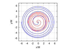
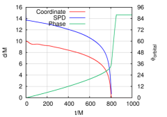
Figure 1: The trajectories of the two black holes, as well as the time dependence of the orbital separation (coordinate and simple proper distance) and phase.

Note that we did not need to use an eccentricity reduction procedure like Pfeiffer et al. (2007); Buonanno et al. (2011); Purrer et al. (2012); Buchman et al. (2012) (although, this would be possible). Rather, the initial data obtained using HiSpID with the parameters obtained by setting the radial momentum (pre-solve) and post-solve net linear angular momentum to the values given by Healy et al. (2017b) is sufficient to obtain binaries with eccentricity $\sim 0.001$. This shows that the improved procedure of Healy et al. (2017b) to provide quasicircular orbits, tested for lowers spins, also holds for the high spin binary here considered.

The waveform of the leading (2,2) mode is shown in Fig. 2. We extract $\psi_{4}$ directly from the simulations, and then compute the strain $h$ by double integration over time. Note that at the relevant scale of the waveform, the initial burst of radiation from our initial data is relatively small, almost invisible. This is in contrast for what is observed in Bowen-York or other conformally flat initial data, where for high spins, of the order of $0.9$, the initial burst can have an amplitude comparable to that of the merger of the two black holes and lead to serious contaminations of the evolution. Besides, Bowen-York data cannot reach spin values of $0.95$ as shown in this paper, since it is limited by spins below $0.93$ Cook and York (1990); Dain et al. (2002); Lousto et al. (2012).

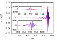
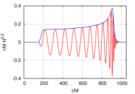
Figure 2: The (2,2) mode of $\psi_{4}$, its amplitude and reconstructed strain $h_{22}$ as measured by an observer at location $r=102.6M$. The strain in the right panel is extrapolated to infinite observer location using the analytic perturbative extrapolation described in Nakano et al. (2015).

From the waveforms we compute the radiated energy and radiated linear and angular momentum using the formulas given in Campanelli and Lousto (1999); Lousto and Zlochower (2007). The recoil of the remnant is given by $-\delta\vec{P}/M_{\rm rem}$, where $\delta\vec{P}$ is the radiated linear momentum and $M_{\rm rem}$ is the mass of the remnant black hole. Our results are summarized in Fig. 3.

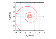
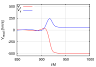
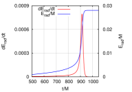
Figure 3: (left) The evolution in velocity space of the recoil vector during the inspiral. (middle) The cumulative recoil versus time. (right) The instantaneous radiated power and cumulative radiated energy versus time. All calculated at infinite observer location.

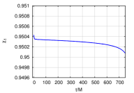
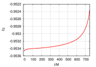
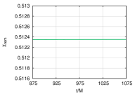
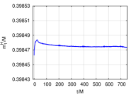
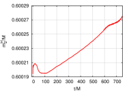
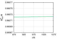
Figure 4: The dimensionless spin (top) and horizon (Christodoulou) mass (bottom) for the two horizons in the binary and the final remnant black hole. The $y$-scale for the mass and spins is set by black hole 2 and is kept the same for the other two black holes.

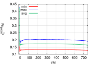
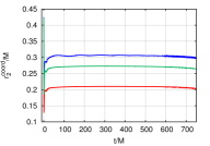
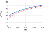
Figure 5: The coordinate radii (minimum, maximum and average) of the three horizons versus time for the full simulation. Note that there is an extremely rapid evolution of the horizon size and shape during the first few $M$ of evolution.

Table 2: Remnant quantities and comparison to fitting formulas. $M_{\rm rem}/M_{\rm equi}$ and $\chi_{\rm rem}$ are the final mass and spin of the remnant measured on the horizon. $V_{\rm recoil}$ and $L_{\rm peak}$ are the recoil velocity in km/s and the peak Luminosity in dimensionless units, measured at infinite observer location. $M_{\rm equi}\omega^{\rm peak}_{22}$ and $|r/M_{\rm equi}H^{\rm peak}_{22}|$ are the peak frequency and amplitude of the 22 mode of the strain. The equilibrium mass $M_{\rm equi}=m_{1}^{\rm equi}+m_{2}^{\rm equi}=0.9987\pm 0.0009$ is used for :normalization.

Quantity	Measured	Fit	% difference
$M_{\rm rem}/M_{\rm equi}$	$0.9620\pm 0.0009$	0.9620	0.00%
$\chi_{\rm rem}$	$0.512350\pm 0.000002$	0.510031	0.45%
$V_{\rm recoil}$	$500.10\pm 0.49$	497.6	0.50%
$L_{\rm peak}(\times 10^{4})$	$7.952\pm 0.0177$	$7.840$	1.40%
$M_{\rm equi}\omega^{\rm peak}_{22}$	$0.3278\pm 0.0019$	0.3309	0.90%
$|r/M_{\rm equi}H^{\rm peak}_{22}|$	$0.3749\pm 0.0010$	0.3743	0.16%

III.1 Diagnostics

One of the most important diagnostics for a black-hole-binary simulation is the degree to which the constraints are satisfied and to what degree the horizon masses and spins are conserved. In Fig. 4, we show the individual horizon mass and dimensionless spin during the evolution, as well as the remnant mass and spin post-merger. Due to our grid configuration, the smaller black hole was actually better resolved. Consequently, the spin of the smaller black hole was actually conserved to a better degree. The spin of the smaller black hole decreased slowly for a net change of 0.0002, or $0.02\%$., the larger black hole, on the other hand, showed a spin decrease (in magnitude) of 0.001, or $0.1\%$. The smaller black hole’s mass varied by less than $0.005\%$, while the larger black hole’s mass increased by $0.013\%$. Note that prior to merger, the spins are within $\pm 0.003$ of $0.95$ and the masses change by less than 0.13%, etc.

In Fig. 6, we show the $L^{2}$ norm of the Hamiltonian and momentum constraints. Here the $L^{2}$ norm is over the region outside the two horizons (or common horizon) and inside a sphere of radius $30M$. Note how the constraints start small ($5\times 10^{-9}-5\times 10^{-8}$) and quickly increase to $10^{-5}-10^{-4}$. This increase is due to unresolved features in the initial data (i.e., the AMR grid cannot propagate high-frequency data accurately). The constraints then damp to $5\times 10^{-8}-5\times 10^{-7}$ and remain roughly constant from then on.

One method which we found was useful for increasing the run speed was to change the lapse condition. Rather than using the standard 1+log lapse, we use a modified slicing closely related to harmonic slicing. This alternative lapse keeps the horizons at a larger coordinate size than 1+log. However, there is still a rapid decrease in the coordinate size of the horizons at very early time. This rapid change in the gauge (see Fig. 5) may be responsible for the initial jump in the constraint violations seen in Fig. 6.

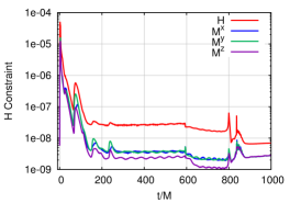
Figure 6: $L^{2}$ norm of the Hamiltonian and momentum constraints versus time. Note the rapid growth during the first 2M of evolution. The CCZ4 damping parameters $\kappa_{1,2}$ managed to suppress the constraint growths during the evolution down to merger and afterwards.

IV Discussion

In this paper we demonstrated that it is possible to evolve unequal-mass black-hole binaries with spins well beyond the Bowen-York limit using the “moving puncture” formalism, and to efficiently generate the initial data for such binaries with low eccentricity without resorting to expensive iterative eccentricity-reduction procedures. This means that comparative studies of these challenging evolutions by the two main methods to numerically solve the field equations of general relativity field equations (the generalized harmonic approach used by SXS and various flavors of the “moving punctures” approach used by many other groups) are now possible beyond the equal-mass case Ruchlin et al. (2017); Zlochower et al. (2017). Independent comparison, along the lines explored in Lovelace et al. (2016), have been very successful in demonstrating the accuracy and correctness of moderate-spin black hole simulations. These new techniques also open the possibility of exploring a region of parameter space which is of high interest for both astrophysical and gravitational wave studies.

In addition, we computed the peak luminosity and frequency, which are key characteristic features of the merger phase of the binary, and have contributed to the remnant final black hole modeling by evaluating the final mass, spin, and recoil of the merged black hole. In particular we have computed the largest recoil velocity recorded of nonprecessing binaries, just above 500 km/s, as predicted by the extrapolation of the formulas given in Healy et al. (2014). The agreement between the extrapolation of the the fitting formulae and the measured values from this simulation, as shown in Table 2, give us a measure of the expected accuracy of this kind of simulations.