On Fermion-Graviton Scattering at Finite Temperature

Abstract

The early universe is dominated by phenomena at high temperatures. The thermal effects decrease during evolution of the universe. However there are some phenomena, such as processes inside stars and black holes, where the role of the temperature is important. Study of processes involving gravitons at finite temperature is a viable means to understand gravitational processes in the universe. Using the Thermo Field Dynamics formalism transition amplitudes involving gravitons and fermions at finite temperature are calculated. In this approach our results consist of two parts: one corresponding to the zero temperature part and the other corresponding to a temperature dependent part.

I Introduction

In the beginning of the Universe gravity exhibits quantum features at extremely high temperatures. For instance during the inflation epoch it is possible that time and temperature worked as entangled quantities infla . The quantum effects at high temperature have been analyzed in Kaluza-Klein cosmology htkk . The classical theories of gravity, Einstein (general) theory and teleparallel gravity, have provided in depth understanding of the universe at zero temperature. The teleparallel gravity, formulated in terms of torsion, is an alternative theory of gravitation and dynamically equivalent to Einstein relativity, in terms of the curvature of space Einst ; Maluf . The difference between them resides in the definition of gravitational energy and angular momentum. It is interesting to note that the graviton propagator obtained from the teleparallel Lagrangian density is different from the one generated in general relativity. Recently the scattering of gravitons and fermions in the framework of teleparallel gravity sfg was considered. However still finite temperature needs to be incorporated in these scattering processes.

In order to treat the dynamics of systems properly temperature has to be incorporated. Temperature effects may be introduced by two equivalent methods: (i) the imaginary time formalism or the Matsubara formalism Matsubara and (ii) the real time formalisms. There are two distinct, but equivalent methods: (a) the closed time path formalism Schwinger and (b) the Thermo Field Dynamics (TFD) method Umezawa1 ; Umezawa2 ; Umezawa22 ; Khanna1 ; Khanna2 . Here the TFD method is chosen. In this formalism the expectation value of a physical observable $A$ in a thermal vacuum, $|0(\beta)\rangle$, is interpreted as the statistical average, i.e., $\langle 0(\beta)|A|0(\beta)\rangle=\langle A\rangle$, where $\beta=\frac{1}{k_{B}T}$ with $T$ being the temperature and $k_{B}$ the Boltzmann constant. In order to satisfy this relation between expectation value of $A$ in a thermal vacuum and statistical average, $\langle A\rangle$, is necessary to extend the usual Hilbert space $S$ to $S_{T}=S\otimes\tilde{S}$, where $\tilde{S}$ is a fictitious Hilbert space. These two spaces are connected by Bogoliubov transformations, which introduce temperature effects. The Bogoliubov transformation introduces a rotation in the tilde and nontilde operators. In addition, the propagators in TFD are written as the sum of two parts: one part of the propagator is zero temperature while the other corresponds to the finite temperature.

The paper is structured in the following form. In section II, the Lagrangian density describes a free fermion and graviton field and the interaction between them. In section III, the Thermo Field Dynamics is introduced. In sections IV and V, the graviton and fermion propagators at finite temperature are presented. In section VI, the interaction between gravitons and fermions at finite temperature is analyzed. Finally in the last section some concluding remarks are presented.

II Lagrangian Density

In this section the lagrangian density of the interacting teleparallel gravity and fermionic field is presented. Here gravitation is described by teleparallelism formalism. Such a theory is formulated in terms of the tetrad field, which is related to the metric, $g_{\mu\nu}=e^{a}\,_{\mu}e_{a\nu}$, in a space-time with torsion. This space-time is called Weitzenböck space which is endowed with Cartan connection, $\Gamma_{\mu\lambda\nu}=e_{a\mu}\partial_{\lambda}e^{a}\,_{\nu}$. The skew symmetric part of the torsion is

$$T^{a}\,_{\lambda\nu}=\partial_{\lambda}e^{a}\,_{\nu}-\partial_{\nu}e^{a}\,_{\lambda}\,.$$ (1)

In the tetrad field latin indices, $a$, represent the Lorentz group and greek indices, $\mu$, indicate the transformation of coordinates. The Cartan connection satisfies the identity

$$\Gamma_{\mu\lambda\nu}={}^{0}\Gamma_{\mu\lambda\nu}+K_{\mu\lambda\nu}\,,$$ (2)

where

$$K_{\mu\lambda\nu} = \frac{1}{2}(T_{\lambda\mu\nu}+T_{\nu\lambda\mu}+T_{\mu\lambda\nu})$$ (3)

is the contortion tensor. Now it is possible to relate the torsion tensor to the scalar curvature defined in a Riemann space. As a consequence the Hilbert-Einstein Lagrangian density assumes the following form in Weitzenböck space

$$eR({}^{0}\Gamma)\equiv-e(\frac{1}{4}T^{abc}T_{abc}+\frac{1}{2}T^{abc}T_{bac}-T^{a}T_{a})+2\partial_{\mu}(eT^{\mu})\,,$$ (4)

where $e$ is the determinant of the tetrad field, $T_{a}=T^{b}\,_{ba}$ and $T_{abc}=e_{b}\,^{\mu}e_{c}\,^{\nu}T_{a\mu\nu}$. If the last term (total divergence) is dropped, since it does not affect the field equation, then the gravitational Lagrangian density is

$${\cal L}_{G}=-ke(\frac{1}{4}T^{abc}T_{abc}+\frac{1}{2}T^{abc}T_{bac}-T^{a}T_{a})\,,$$ (5)

where $k=1/16\pi$. It can be rewritten as

$${\cal L}_{G}\equiv-ke\Sigma^{abc}T_{abc}\,,$$ (6)

where

$$\Sigma^{abc}=\frac{1}{4}(T^{abc}+T^{bac}-T^{cab})+\frac{1}{2}(\eta^{ac}T^{b}-\eta^{ab}T^{c})\,.$$ (7)

Since this Lagrangian density is equivalent to that of Einstein relativity: then both theories are dynamically equivalent. Hence this Lagrangian density $({\cal L}_{G})$ is used to calculate all processes related to gravitons.

The complete Lagrangian density that describes the interaction between gravitons and fermions is given by

$${\cal L}={\cal L}_{G}+{\cal L}_{M},$$ (8)

where ${\cal L}_{M}$ stands for the fermion field coupled to gravity. It is given by

$${\cal L}_{M}=e\left[\frac{i}{2}\left(\bar{\psi}\gamma^{\mu}D_{\mu}\psi-D_{\mu}\bar{\psi}\gamma^{\mu}\psi\right)-m\bar{\psi}\psi\right]\,,$$ (9)

with $D_{\mu}=\partial_{\mu}+\frac{i}{4}\,K_{\mu ab}\Sigma^{ab}$ and $\Sigma^{ab}=\frac{i}{2}[\gamma^{a},\gamma^{b}]$, $\psi$ is the Fermi field with mass $m$, $\bar{\psi}=\psi^{\dagger}\gamma_{0}$ and $\gamma^{\mu}$ are Dirac matrices. Thus the fermionic Lagrangian density is separated into two parts as ${\cal L}_{M}={\cal L}_{F}+{\cal L}_{GF}$, where

$${\cal L}_{F}=e\left[\frac{i}{2}\left(\bar{\psi}\gamma^{\mu}\partial_{\mu}\psi-\partial_{\mu}\bar{\psi}\gamma^{\mu}\psi\right)-m\bar{\psi}\psi\right]\,,$$ (10)

stands for the free fermion field and

$${\cal L}_{GF}=-\frac{e}{8}\left(\bar{\psi}\gamma^{\mu}K_{\mu ab}\Sigma^{ab}\psi+\bar{\psi}K_{\mu ab}\Sigma^{ab}\gamma^{\mu}\psi\right)\,,$$ (11)

describes the interaction between fermions and gravitons.

III Thermo Field Dynamics - TFD

Here a brief introduction to TFD formalism is presented. This formalism is constructed with two ingredients: (i) a doubling of the Fock space, $S$, giving rise to $S_{T}=S\otimes\tilde{S}$, applicable to equilibrium systems. The physical quantities are described by the nontilde operators. (ii) Bogoliubov transformation introduces thermal effects through a rotation in the tilde and nontilde operators. The Bogoliubov transformations for bosons and fermions are distinct.

III.1 For bosons

Bogoliubov transformations for bosons are

$$A_{a\mu}(k) = c_{B}A_{a\mu}(k,\beta)+d_{B}\tilde{A}_{a\mu}^{\dagger}(k,\beta),$$

$$A_{a\mu}^{\dagger}(k) = c_{B}A_{a\mu}^{\dagger}(k,\beta)+d_{B}\tilde{A}_{a\mu}(k,\beta),$$

$$\tilde{A}_{a\mu}(k) = c_{B}\tilde{A}_{a\mu}(k,\beta)+d_{B}A_{a\mu}^{\dagger}(k,\beta),$$

$$\tilde{A}_{a\mu}^{\dagger}(k) = c_{B}\tilde{A}_{a\mu}^{\dagger}(k,\beta)+d_{B}A_{a\mu}(k,\beta),$$ (12)

where $(A_{a\mu}^{\dagger},\tilde{A}_{a\mu}^{\dagger})$ are creation operators, $(A_{a\mu},\tilde{A}_{a\mu})$ are destruction operators and

$$c_{B}^{2}=1+f_{B}(\omega),\quad\quad d_{B}^{2}=f_{B}(\omega),\quad\quad f_{B}(\omega)=\frac{1}{e^{\beta\omega}-1}.$$ (13)

Here $\omega=\omega(k)$. These thermal operators satisfy the algebraic relations

$$\left[A_{a\mu}(k,\beta),A_{b\nu}^{\dagger}(p,\beta)\right] = \delta^{3}(k-p)\eta_{ab}\,g_{\mu\nu},$$

$$\left[\tilde{A}_{a\mu}(k,\beta),\tilde{A}_{b\nu}^{\dagger}(p,\beta)\right] = \delta^{3}(k-p)\eta_{ab}\,g_{\mu\nu},$$ (14)

and other commutation relations are null.

III.2 For fermions

Bogoliubov transformations for fermions are

$$A_{a\mu}(k) = c_{F}A_{a\mu}(k,\beta)+d_{F}\tilde{A}_{a\mu}^{\dagger}(k,\beta),$$

$$A_{a\mu}^{\dagger}(k) = c_{F}A_{a\mu}^{\dagger}(k,\beta)+d_{F}\tilde{A}_{a\mu}(k,\beta),$$

$$\tilde{A}_{a\mu}(k) = c_{F}\tilde{A}_{a\mu}(k,\beta)-d_{F}A_{a\mu}^{\dagger}(k,\beta),$$

$$\tilde{A}_{a\mu}^{\dagger}(k) = c_{F}\tilde{A}_{a\mu}^{\dagger}(k,\beta)-d_{F}A_{a\mu}(k,\beta),$$ (15)

with

$$c_{F}^{2}=1-f_{F}(\omega),\quad\quad d_{F}^{2}=f_{F}(\omega),\quad\quad f_{F}(\omega)=\frac{1}{e^{\beta\omega}+1}.$$ (16)

In this case the algebraic relations are

$$\left\{A_{a\mu}(k,\beta),A_{b\nu}^{\dagger}(p,\beta)\right\} = \delta^{3}(k-p)\eta_{ab}\,g_{\mu\nu},$$

$$\left\{\tilde{A}_{a\mu}(k,\beta),\tilde{A}_{b\nu}^{\dagger}(p,\beta)\right\} = \delta^{3}(k-p)\eta_{ab}\,g_{\mu\nu}.$$ (17)

Other commutation relations are null.

IV The Graviton Propagator at finite temperature

The graviton propagator in weak field approximation is defined as

$$iD^{kl}_{ab\mu\nu}(x-y)=\left\langle 0(\beta)\left|\tau\left[e^{k}_{a\mu}(x)e^{l}_{b\nu}(y)\right]\right|0(\beta)\right\rangle,$$ (18)

where $\tau$ is the time ordering operator, $k,l=1,2$ and $a,b,\mu,\nu$ are tensor indices. In this approximation $g_{\mu\nu}=\eta_{\mu\nu}+h_{\mu\nu}$. In teleparallel gravity the fundamental tetrad field is $e_{a\mu}(x)$. A Fourier expansion of this field is written as

$$e_{a\mu}(x)=\int\frac{d^{3}k}{\sqrt{2\omega_{k}(2\pi)^{3}}}\left(A_{a\mu}(k)e^{-ik_{\sigma}x^{\sigma}}+A_{a\mu}^{\dagger}(k)e^{ik_{\sigma}x^{\sigma}}\right),$$ (19)

where $A_{a\mu}(k)$ and $A_{a\mu}^{\dagger}(k)$ are the annihilation and creation operators, respectively.

The propagator in TFD is a thermal doublet and has 2$\times$2 matrix structure. Using the thermal doublet notation,

$$\left(\begin{array}[]{cc}e_{a\mu}^{1}\\ e_{a\mu}^{2}\end{array}\right)=\left(\begin{array}[]{cc}e_{a\mu}\\ \tilde{e}_{a\mu}^{\dagger}\end{array}\right),$$ (24)

the component $k=l=1$ is written explicitly as

$$iD^{11}_{ab\mu\nu}(x-y) = \theta(t_{x}-t_{y})\left\langle 0(\beta)\left|\left[e_{a\mu}(x)e_{b\nu}(y)\right]\right|0(\beta)\right\rangle$$ (25)

$$+ \theta(t_{y}-t_{x})\left\langle 0(\beta)\left|\left[e_{b\nu}(y)e_{a\mu}(x)\right]\right|0(\beta)\right\rangle,$$

where $\theta(t_{x}-t_{y})$ is the step function. For simplicity, the components are calculated separately. Substituting the fundamental field, eq. (19), the 11-component of the propagator becomes

$$iD^{11}_{ab\mu\nu}(x-y) = \theta(t_{x}-t_{y})\int\frac{d^{3}k}{\sqrt{2\omega_{k}(2\pi)^{3}}}\int\frac{d^{3}p}{\sqrt{2\omega_{p}(2\pi)^{3}}}\times$$

$$\times \langle 0(\beta)|(A_{a\mu}(k)e^{-ik_{\sigma}x^{\sigma}}+A_{a\mu}^{\dagger}(k)e^{ik_{\sigma}x^{\sigma}})(A_{b\nu}(p)e^{-ip_{\sigma}y^{\sigma}}+A_{b\nu}^{\dagger}(p)e^{ip_{\sigma}y^{\sigma}})|0(\beta)\rangle$$

$$+ \theta(t_{y}-t_{x})\int\frac{d^{3}p}{\sqrt{2\omega_{p}(2\pi)^{3}}}\int\frac{d^{3}k}{\sqrt{2\omega_{k}(2\pi)^{3}}}\times$$

$$\times \langle 0(\beta)|(A_{b\nu}(p)e^{-ip_{\sigma}y^{\sigma}}+A_{b\nu}^{\dagger}(p)e^{ip_{\sigma}y^{\sigma}})(A_{a\mu}(k)e^{-ik_{\sigma}x^{\sigma}}+A_{a\mu}^{\dagger}(k)e^{ik_{\sigma}x^{\sigma}})|0(\beta)\rangle.$$

Using the Bogoliubov transformations, eqs. (12), we get

$$iD^{11}_{ab\mu\nu}(x-y) = \theta(t_{x}-t_{y})\int\frac{d^{3}k}{\sqrt{2\omega_{k}(2\pi)^{3}}}\int\frac{d^{3}p}{\sqrt{2\omega_{p}(2\pi)^{3}}}\times$$

$$\times \langle 0(\beta)|[c_{B}^{2}A_{a\mu}(k)A_{b\nu}^{\dagger}(p)e^{-ik_{\sigma}x^{\sigma}+ip_{\sigma}y^{\sigma}}+d_{B}^{2}\tilde{A}_{a\mu}(k)\tilde{A}_{b\nu}^{\dagger}(p)e^{ik_{\sigma}x^{\sigma}-ip_{\sigma}y^{\sigma}}]|0(\beta)\rangle$$

$$+ \theta(t_{y}-t_{x})\int\frac{d^{3}p}{\sqrt{2\omega_{p}(2\pi)^{3}}}\int\frac{d^{3}k}{\sqrt{2\omega_{k}(2\pi)^{3}}}\times$$

$$\times \langle 0(\beta)|[c_{B}^{2}A_{b\nu}(p)A_{a\mu}^{\dagger}(k)e^{-ip_{\sigma}y^{\sigma}+ik_{\sigma}x^{\sigma}}+d_{B}^{2}\tilde{A}_{b\nu}(p)\tilde{A}_{a\mu}^{\dagger}(k)e^{ip_{\sigma}y^{\sigma}-ik_{\sigma}x^{\sigma}}]|0(\beta)\rangle.$$

Assuming that commutation relations, eqs. (14), are satisfied, this component of the graviton propagator becomes

$$iD^{11}_{ab\mu\nu}(x-y) = -\int\frac{d^{3}k}{(2\pi)^{3}}\frac{1}{2\omega_{k}}\eta_{ab}\,\eta_{\mu\nu}\Biggl{\{}c_{B}^{2}\Bigl{[}\theta(t_{x}-t_{y})e^{-ik_{\sigma}(x^{\sigma}-y^{\sigma})}+\theta(t_{y}-t_{x})e^{ik_{\sigma}(x^{\sigma}-y^{\sigma})}\Bigl{]}$$ (28)

$$+ d_{B}^{2}\Bigl{[}\theta(t_{x}-t_{y})e^{ik_{\sigma}(x^{\sigma}-y^{\sigma})}+\theta(t_{y}-t_{x})e^{-ik_{\sigma}(x^{\sigma}-y^{\sigma})}\Bigl{]}\Biggl{\}},$$

where the integral over $d^{3}p$ has been calculated. Using the Cauchy theorem

$$\int dk^{0}\frac{e^{-ik_{0}(x_{0}-y_{0})}}{k_{0}-(\omega_{k}-i\xi)} = -2\pi ie^{-i\omega_{k}(x_{0}-y_{0})}\theta(x_{0}-y_{0}),$$

$$\int dk^{0}\frac{e^{-ik_{0}(x_{0}-y_{0})}}{k_{0}-(-\omega_{k}+i\xi)} = 2\pi ie^{i\omega_{k}(x_{0}-y_{0})}\theta(y_{0}-x_{0}),$$ (29)

the 11-component is given as

$$D^{11}_{ab\mu\nu}(x-y) = -\int\frac{d^{4}k}{(2\pi)^{4}}e^{-ik_{\sigma}(x^{\sigma}-y^{\sigma})}\eta_{ab}\,\eta_{\mu\nu}\left[\frac{c_{B}^{2}}{k_{0}^{2}-(\omega_{k}-i\epsilon)^{2}}-\frac{d_{B}^{2}}{k_{0}^{2}-(\omega_{k}+i\epsilon)^{2}}\right].$$ (30)

Similarly the component $k=1$ and $l=2$ is written as

$$iD^{12}_{ab\mu\nu}(x-y) = \theta(t_{x}-t_{y})\langle 0(\beta)|[e_{a\mu}(x)\tilde{e}_{b\nu}^{\dagger}(y)]|0(\beta)\rangle$$ (31)

$$+ \theta(t_{y}-t_{x})\langle 0(\beta)|[\tilde{e}_{b\nu}^{\dagger}(y)e_{a\mu}(x)]|0(\beta)\rangle.$$

Following similar steps used for the 11-component, we get

$$D^{12}_{ab\mu\nu}(x-y) = -\int\frac{d^{4}k}{(2\pi)^{4}}e^{-ik_{\sigma}(x^{\sigma}-y^{\sigma})}\eta_{ab}\,\eta_{\mu\nu}\left[\frac{c_{B}d_{B}}{k_{0}^{2}-(\omega_{k}-i\epsilon)^{2}}-\frac{c_{B}d_{B}}{k_{0}^{2}-(\omega_{k}+i\epsilon)^{2}}\right].$$ (32)

Then for the component $k=2$ and $l=1$ we have

$$D^{21}_{ab\mu\nu}(x-y) = D^{12}_{ab\mu\nu}(x-y).$$ (33)

Finally the 22-component is

$$D^{22}_{ab\mu\nu}(x-y) = -\int\frac{d^{4}k}{(2\pi)^{4}}e^{-ik_{\sigma}(x^{\sigma}-y^{\sigma})}\eta_{ab}\,\eta_{\mu\nu}\left[\frac{d_{B}^{2}}{k_{0}^{2}-(\omega_{k}-i\epsilon)^{2}}-\frac{c_{B}^{2}}{k_{0}^{2}-(\omega_{k}+i\epsilon)^{2}}\right].$$ (34)

The graviton propagator at finite temperature is

$$D^{kl}_{ab\mu\nu}(x-y)=i\int\frac{d^{4}k}{(2\pi)^{4}}e^{-ik_{\sigma}(x^{\sigma}-y^{\sigma})}\,D^{kl}_{ab\mu\nu}(k),$$ (35)

where

$$-iD^{kl}_{ab\mu\nu}(k)=\left(\begin{array}[]{cc}\frac{c_{B}^{2}}{k_{0}^{2}-(\omega_{k}-i\epsilon)^{2}}-\frac{d_{B}^{2}}{k_{0}^{2}-(\omega_{k}+i\epsilon)^{2}}&\hskip 5.69046pt\frac{c_{B}d_{B}}{k_{0}^{2}-(\omega_{k}-i\epsilon)^{2}}-\frac{c_{B}d_{B}}{k_{0}^{2}-(\omega_{k}+i\epsilon)^{2}}\\ \frac{c_{B}d_{B}}{k_{0}^{2}-(\omega_{k}-i\epsilon)^{2}}-\frac{c_{B}d_{B}}{k_{0}^{2}-(\omega_{k}+i\epsilon)^{2}}&\hskip 5.69046pt\frac{d_{B}^{2}}{k_{0}^{2}-(\omega_{k}-i\epsilon)^{2}}-\frac{c_{B}^{2}}{k_{0}^{2}-(\omega_{k}+i\epsilon)^{2}}\end{array}\right)\,\eta_{ab}\,\eta_{\mu\nu}.$$ (38)

Using relations given in eq. (13), the propagator is separated as

$$-iD^{kl}_{ab\mu\nu}(k)=-iD^{kl}_{(0)ab\mu\nu}(k)-iD^{kl}_{(\beta)ab\mu\nu}(k),$$ (39)

where $D^{kl}_{(0)ab\mu\nu}(k)$ and $D^{kl}_{(\beta)ab\mu\nu}(k)$ are zero and finite temperature components respectively. Explicitly

$$-iD^{kl}_{(0)ab\mu\nu}(k)=\eta_{ab}\,\eta_{\mu\nu}\left[k_{0}^{2}-(\omega_{k}-i\epsilon\xi)^{2}\right]^{-1}\xi$$ (40)

and

$$-iD^{kl}_{(\beta)ab\mu\nu}(k)=-\eta_{ab}\,\eta_{\mu\nu}\frac{2\pi i\delta(k_{0}^{2}-\omega_{k}^{2})}{e^{\beta\omega_{k}}-1}\left(\begin{array}[]{cc}1&e^{\beta\omega_{k}/2}\\ e^{\beta\omega_{k}/2}&1\end{array}\right),$$ (43)

where

$$\xi=\left(\begin{array}[]{cc}1&0\\ 0&-1\end{array}\right).$$ (46)

The 11-component yields the physical graviton propagator at zero temperature as

$$D_{ab\mu\nu}(k)=\frac{i\eta_{ab}}{k^{\mu}k^{\nu}}.$$ (47)

V The Electron Propagator at Finite temperature

The electron propagator is defined as

$$S^{kl}_{\mu\nu}(x-y) = \theta(t_{x}-t_{y})\langle 0(\beta)|\psi^{k}_{\mu}(x)\bar{\psi}^{l}_{\nu}(y)|0(\beta)\rangle$$ (48)

$$- \theta(t_{y}-t_{x})\langle 0(\beta)|\bar{\psi}^{l}_{\nu}(y)\psi^{k}_{\mu}(x)|0(\beta)\rangle,$$

where $\bar{\psi}(y)=\psi^{\dagger}(y)\gamma^{0}$ and $\mu,\nu$ are the spinor indices. Using

$$\psi(x)=\sum_{r}\int d^{3}k\,\left[u^{r}(k)a^{r}(k)e^{i(k\cdot x-\xi_{k}t)}+v^{r}(k)b^{r\dagger}(k)e^{-i(k\cdot x-\xi_{k}t)}\right],$$ (49)

where $a^{r}(k)$ and $b^{r}(k)$ are annihilation operators for electrons and positrons, respectively, and Dirac spinors are $u^{r}(k)$ and $v^{r}(k)$. Then the electron propagator at finite temperature becomes AF

$$S^{ab}_{\mu\nu}(k) = \left(\frac{\gamma^{0}\xi-\vec{\gamma}\cdot\vec{k}+m}{2\xi}\right)_{\mu\nu}\left[U_{F}(\xi)(k_{0}-\xi+i\delta\tau)^{-1}U_{F}^{\dagger}(\xi)\right]^{ab}$$ (50)

$$+ \left(\frac{\gamma^{0}\xi+\vec{\gamma}\cdot\vec{k}-m}{2\xi}\right)_{\mu\nu}\left[U_{F}(-\xi)(k_{0}+\xi+i\delta\tau)^{-1}U_{F}^{\dagger}(-\xi)\right]^{ab},$$

where Bogoliubov transformations, eqs. (15), are used. Here $\xi\equiv\xi(k)$ and

$$U_{F}(\xi)=\left(\begin{array}[]{cc}c_{F}(\xi)&d_{F}(\xi)\\ -d_{F}(\xi)&c_{F}(\xi)\end{array}\right),$$ (53)

with $c_{F}(\xi)$ and $d_{F}(\xi)$ are given by eq. (16).

The electron propagator is separated into two parts as

$$S_{\mu\nu}(k)=S_{\mu\nu}^{(0)}(k)+S_{\mu\nu}^{(\beta)}(k),$$ (54)

where $S_{\mu\nu}^{(0)}(k)$ and $S_{\mu\nu}^{(\beta)}(k)$ are zero and finite temperature parts respectively. Explicitly

$$-iS_{\mu\nu}^{(0)}(k) = \frac{\not{k}+m}{k^{2}-m^{2}},$$ (55)

$$-iS_{\mu\nu}^{(\beta)}(k) = \frac{2\pi i}{e^{\beta k_{0}}+1}\Biggl{[}\frac{\gamma^{0}\epsilon-\vec{\gamma}\cdot\vec{k}+m}{2\epsilon}\left(\begin{array}[]{cc}1&e^{\beta k_{0}/2}\\ e^{\beta k_{0}/2}&-1\end{array}\right)\delta(k_{0}-\epsilon)$$ (58)

$$+ \frac{\gamma^{0}\epsilon+\vec{\gamma}\cdot\vec{k}-m}{2\epsilon}\left(\begin{array}[]{cc}-1&e^{\beta k_{0}/2}\\ e^{\beta k_{0}/2}&1\end{array}\right)\delta(k_{0}+\epsilon)\Biggl{]}.$$ (61)

VI Gravitons-Fermions interactions

In this section transition amplitudes, ${\cal M}$, for the M$\varnothing$ller scattering, the Compton scattering and a new gravitational scattering process are calculated.

VI.1 Propagators

The graviton and fermion propagators are represented in FIG.1 and FIG.2, respectively.

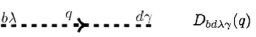
Figure 1: Graviton propagator

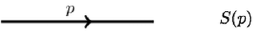
Figure 2: Electron propagator

VI.2 Vertex factors

The vertex of the interaction between two gravitons and two fermions is

$$V^{ab\sigma\nu}=\frac{ie}{8}\Sigma^{ab}\eta^{\sigma\nu}\left(\gamma^{\mu}q_{2\mu}+q_{2\mu}\gamma^{\mu}\right),$$ (62)

and is represented in FIG.3.

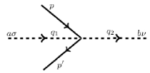
Figure 3: Graviton-Fermion Vertex

The fermion-graviton vertex is

$${\cal V}^{b\sigma}=\frac{ie}{4}\Sigma^{b\sigma}\left(\gamma^{\mu}q_{\mu}+q_{\mu}\gamma^{\mu}\right),$$ (63)

where the approximation $e_{a\nu}=\delta_{a\nu}+\phi_{a\nu}$, with $\delta_{a\nu}$ being the Kronecker delta and a weak field approximation for $\phi_{a\nu}$ is used sfg . This vertex is represented in FIG.4.

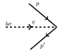
Figure 4: Graviton-Fermion Vertex

VI.3 Transition amplitudes at finite temperature

VI.3.1 M$\varnothing$ller scattering

The M$\varnothing$ller scattering process is described in FIG. 5.

Figure 5: M$\varnothing$ller scattering

The transition amplitude is

$$-i{\cal M}=\bar{u}(p_{2}){\cal V}^{b\sigma}u(p_{1})D_{bd\sigma\gamma}(q)\bar{u}(p_{4}){\cal V}^{d\gamma}u(p_{3}),$$ (64)

where ${\cal V}^{b\sigma}$ is the vertex and $D_{bd\sigma\gamma}(q)$ is the graviton propagator at finite temperature. The transition amplitude for this scattering consist of two parts

$${\cal M}={\cal M}_{(0)}+{\cal M}_{(\beta)},$$ (65)

where ${\cal M}_{(0)}$ and ${\cal M}_{(\beta)}$ are zero and finite temperature components respectively. Zero temperature transition amplitude is

$${\cal M}_{(0)} = \frac{e^{2}}{16}\bar{u}(p_{2})u(p_{1})\left(\gamma^{\mu}q_{\mu}+q_{\mu}\gamma^{\mu}\right)\Sigma_{d}\,^{\sigma}\Sigma^{d}\,_{\sigma}\times$$ (66)

$$\times \left[\frac{\xi}{q_{0}^{2}-(\omega_{q}-i\epsilon\xi)^{2}}\right]\left(\gamma^{\nu}q_{\nu}+q_{\nu}\gamma^{\nu}\right)\bar{u}(p_{4})u(p_{3}),$$

and the finite temperature part is

$${\cal M}_{(\beta)} = \frac{e^{2}}{16}\bar{u}(p_{2})u(p_{1})\left(\gamma^{\mu}q_{\mu}+q_{\mu}\gamma^{\mu}\right)\Sigma_{d}\,^{\sigma}\Sigma^{d}\,_{\sigma}\times$$ (69)

$$\times \left[\frac{2\pi i\delta(q_{0}^{2}-\omega_{q}^{2})}{e^{\beta\omega_{q}}-1}\left(\begin{array}[]{cc}1&e^{\beta\omega_{q}/2}\\ e^{\beta\omega_{q}/2}&1\end{array}\right)\right]\left(\gamma^{\nu}q_{\nu}+q_{\nu}\gamma^{\nu}\right)\bar{u}(p_{4})u(p_{3}),$$

where $\Sigma_{d}\,^{\sigma}\Sigma^{d}\,_{\sigma}=\eta_{bd}\,\eta_{\sigma\gamma}\Sigma^{d\sigma}\Sigma^{d\gamma}$.

VI.3.2 Compton scattering

The Compton scattering process is given in FIG. 6.

Figure 6: Compton scattering

The transition amplitude is

$$-i{\cal M}=\bar{u}(p_{2}){\cal V}^{b\sigma}S(p)\eta_{bc}\,\eta_{\sigma\nu}{\cal V}^{c\mu}u(p_{1}),$$ (70)

then

$${\cal M} = \frac{e^{2}}{16}\bar{u}(p_{2})\Sigma^{b\sigma}\left(\gamma^{\mu}q_{1\mu}+q_{1\mu}\gamma^{\mu}\right)\Sigma_{b\sigma}\left(\gamma^{\alpha}q_{2\alpha}+q_{2\alpha}\gamma^{\alpha}\right)u(p_{1})\times$$ (73)

$$\times \Biggl{\{}\left(\frac{\not{p}+m}{p^{2}-m^{2}}\right)+\frac{2\pi i}{e^{\beta p_{0}}+1}\Biggl{[}\frac{\gamma^{0}\epsilon-\vec{\gamma}\cdot\vec{p}+m}{2\epsilon}\left(\begin{array}[]{cc}1&e^{\beta p_{0}/2}\\ e^{\beta p_{0}/2}&-1\end{array}\right)\delta(p_{0}-\epsilon)$$

$$+ \frac{\gamma^{0}\epsilon+\vec{\gamma}\cdot\vec{p}-m}{2\epsilon}\left(\begin{array}[]{cc}-1&e^{\beta p_{0}/2}\\ e^{\beta p_{0}/2}&1\end{array}\right)\delta(p_{0}+\epsilon)\Biggl{]}\Biggl{\}}.$$ (76)

Here the first part corresponds to the zero temperature case and the second and third parts are finite temperature effects.

VI.3.3 A gravitational scattering at finite temperature

In the framework of the teleparallel gravity, there is a particular scattering process as given in FIG. 7.

Figure 7: A gravitational scattering

For this process the transition amplitude is

$$-i{\cal M}=\bar{u}(p_{2}){\cal V}^{b\sigma}u(p_{1})D_{bd\sigma\gamma}(q_{2})\bar{u}(p_{4}){\cal V}^{d\gamma}u(p_{3}),$$ (77)

which at finite temperature yields

$${\cal M} = \frac{e^{2}}{16}\bar{u}(p_{2})\left(\gamma^{\mu}q_{1\mu}+q_{1\mu}\gamma^{\mu}\right)u(p_{1})\Sigma_{d}\,^{\sigma}\Sigma^{d}_{\sigma}\,\bar{u}(p_{4})\left(\gamma^{\nu}q_{3\nu}+q_{3\nu}\gamma^{\nu}\right)u(p_{3})\times$$ (80)

$$\times \left[\frac{\xi}{q_{20}^{2}-(\omega_{2q}-i\epsilon\xi)^{2}}+\frac{2\pi i\delta(q_{20}^{2}-\omega_{2q}^{2})}{e^{\beta\omega_{2q}}-1}\left(\begin{array}[]{cc}1&e^{\beta\omega_{2q}/2}\\ e^{\beta\omega_{2q}/2}&1\end{array}\right)\right].$$

The first term corresponds to the zero temperature results and the second part is finite temperature effects.

VII Conclusions

Transition amplitudes for interactions of fermions and gravitons are calculated at finite temperature. The gravitons are described by the teleparallel gravity in the weak field approximation, an alternative theory of gravitation which is formulated in a space with torsion. Teleparallel gravity provides a viable expression to deal with the interaction of gravitons and fermions since their coupling is due to the contorsion. The temperature of such processes is introduced by Thermo Field Dynamics which has the advantage of preserving the temporal coordinate. The scattering between gravitons and fermions at finite temperature may have been important in the formation of matter in the development of the universe when the temperature was higher and effects of quantum gravity were relevant.