Bukhvostov-Lipatov model
and quantum-classical duality
Vladimir V. Bazhanov1, Sergei L. Lukyanov2,3
and
Boris A. Runov1,4
1Department of Theoretical Physics,
Research School of Physics and Engineering,
Australian National University, Canberra, ACT 2601, Australia
2NHETC, Department of Physics and Astronomy,
Rutgers University,
Piscataway, NJ 08855-0849, USA
3Kharkevich Institute for Information Transmission Problems,
Moscow, 127994 Russia
and
4Institute for Theoretical and Experimental Physics,
Moscow, 117218, Russia
Abstract
The Bukhvostov-Lipatov model is an exactly soluble model of two interacting Dirac fermions in 1+1 dimensions. The model describes weakly interacting instantons and anti-instantons in the non-linear sigma model. In our previous work [arXiv:1607.04839] we have proposed an exact formula for the vacuum energy of the Bukhvostov-Lipatov model in terms of special solutions of the classical sinh-Gordon equation, which can be viewed as an example of a remarkable duality between integrable quantum field theories and integrable classical field theories in two dimensions. Here we present a complete derivation of this duality based on the classical inverse scattering transform method, traditional Bethe ansatz techniques and analytic theory of ordinary differential equations. In particular, we show that the Bethe ansatz equations defining the vacuum state of the quantum theory also define connection coefficients of an auxiliary linear problem for the classical sinh-Gordon equation. Moreover, we also present details of the derivation of the non-linear integral equations determining the vacuum energy and other spectral characteristics of the model in the case when the vacuum state is filled by 2-string solutions of the Bethe ansatz equations.
1 Introduction
This paper is a sequel to our previous work [2] devoted to the study of the Bukhvostov-Lipatov (BL) model [1]. Originally, this model was introduced to describe weakly interacting instantons and anti-instantons in the non-linear sigma model in two dimensions, extending the results of [3, 4]. It is an exactly soluble (1+1)-dimensional QFT, containing two interacting Dirac fermions (), defined by the renormalized Lagrangian
| (1.1) |
This model provides a remarkable illustration to the idea of the exact instanton counting. Indeed, as explained in [2], the model can be reformulated as a bosonic QFT with two interacting bosons, which upon an analytic continuation into a strong coupling regime, becomes equivalent to the originating non-linear sigma model.
Our interest to the BL model is also motivated by the study of an intriguing correspondence between Integrable Quantum Field Theories (IQFT) and Integrable Classical Field Theories in two dimensions, which cannot be expected from the standard correspondence principle. Over the past two decades this topic has been continuously developed, as can be seen from the works [5, 6, 7, 8, 9, 10, 11, 12, 13, 14, 15, 16, 17, 18, 19]. The new correspondence yields an extremely efficient extension of the Quantum Inverse Scattering Method (QISM) [20] by connecting it with well-developed techniques of the spectral theory of ordinary differential equations (ODE) and, most importantly, the Classical Inverse Scattering Method [21]. The resulting approach is usually referred to as “ODE/IM” or “ODE/IQFT” correspondence. Ultimately, for a massive IQFT, it allows one to describe quantum stationary states (and the corresponding eigenvalues of quantum integrals of motion) in terms of special singular solutions of classical integrable partial differential equations. To this moment, the approach has already been applied to a number of IQFT models, such as the sine(h)-Gordon model [14], the Bullough-Dodd model [15] and various regimes [16, 17, 22] of the Fateev model [23], including the “sausage model” [24] (a one-parameter deformation of the sigma-model). Despite this progress, the subject, certainly, deserves further studies for a better understanding of the mathematical structure of the ODE/IQFT correspondence, as well as unraveling fundamental underlying reasons of its existence. In this work we continue to address these problems in the case of the BL model. As noted before, this model is integrable. Its coordinate Bethe ansatz solution was presented in the original BL paper [1]. The corresponding factorized scattering theory was proposed in [23]. The non-linear integral equations for calculating the ground state energy were derived in [25].
As in [2] we consider the theory (1.1) in a finite volume imposing twisted (quasiperiodic) boundary conditions on the fundamental fermion fields,
| (1.2) |
The pair of real numbers labels different sectors of the theory and, therefore, one can address the problem of computing of vacuum energy in each sector. The perturbative treatment of (1.1) leads to ultraviolet (UV) divergences. In [2] we used the renormalization procedure which preserves the integrability of the theory. In this case the fermion mass could only have a finite renormalization and the only UV divergent quantity remaining in the theory is the bulk vacuum energy, defined as . Therefore, it is convenient to extract the (divergent) extensive part from and introduce a scaling function
| (1.3) |
which is simply related to the so-called effective central charge, . Notice that it is a dimensionless function of the dimensionless variables and , satisfying the normalization condition .
In [2] the scaling function (1.3) was computed in a variety of different ways. Let us briefly review this work and then describe new considerations contained in this paper. First, we used the renormalized Matsubara perturbation theory (recall that we consider the finite-volume theory) to calculate the first two non-trivial orders of the expansion of the scaling function (1.3) in powers of the coupling constant . The physical fermion mass is normalized by the large distance asymptotics of the scaling function. As for the coupling constant , it is convenient to trade it off the for a physically observable parameter , which enters the -matrix of the model. According to [23] the particle spectrum contains a fundamental quadruplet of mass whose two-particle -matrix is given by the direct product of two -symmetric solutions of the -matrix bootstrap, with . Each of the factors coincides with the soliton -matrix in the quantum sine-Gordon theory with the renormalized coupling constant .
Further, in [2] we also used the conformal perturbation theory and computed the small- expansion of the scaling function (1.3) to within the forth order terms , inclusively. Then, applying rather non-trivial integral identities for the hypergeometric function, we discovered that the result of these perturbative calculations can be expressed through a particular solution of the Liouville equation. Guided by this peculiar observation and the previous results [16, 17, 22] concerning different regimes of the Fateev model we presented an exact formula for the scaling function
| (1.4) |
where , in terms of a real valued solution of the classical sinh-Gordon equation
| (1.5) |
in the domain .
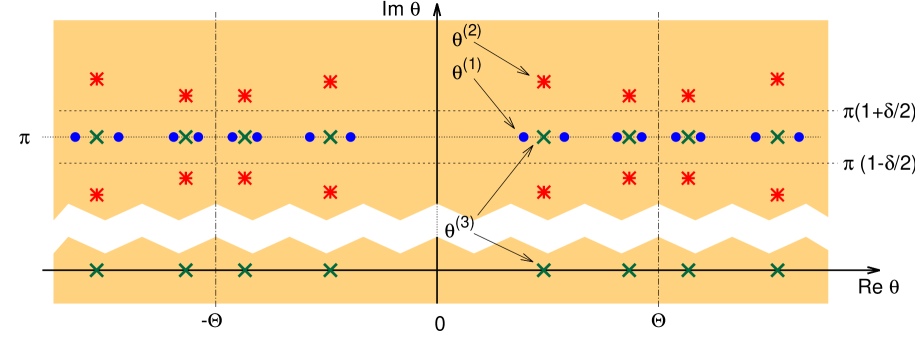
This domain is obtained from two inclined half-infinite strips of the complex plane glued together along their infinite sides, as shown in Fig. 1. It has the topology of a two-dimensional sphere with three punctures . At the singular points on the real axis the solution has the following asymptotic behavior:
| (1.6) |
and
| (1.7) |
The conical angles at the points and (see Fig. 1) are determined by the parameters and , while the number are related to the twists parameters in (1.2). The quantity is the free energy of a free 1D boson, given by
| (1.8) |
where is the (dimensionless) inverse temperature.
In this paper we present a derivation of the formula (1.4). It is based on the fact that the sinh-Gordon equation is a classical integrable equation, which can be treated by the inverse scattering transform method. This allows one to relate the classical conserved charges to the connection coefficients of ODE’s arising in the auxiliary linear problem for the sinh-Gordon equation. It turns out that these connection coefficients are determined by the same Bethe ansatz equations that appear in the coordinate Bethe ansatz solution of the BL model. As a result eigenvalues and eigenstates of QFT integrals motion are determined by solutions of the classical sinh-Gordon equation. In addition, using standard approaches of integrable QFT, we derive another expression for the scaling function in terms of solutions of Non-Linear Integral Equations (NLIE) which are equivalent to Bethe ansatz equations, but more efficient for numerical analysis.
The organization of the paper is as follows. The coordinate Bethe ansatz for the BL model is considered in Sect. 2. The lattice-type regularization of the Bethe ansatz equations and associated particle-hole transformations are considered in Sect. 3. The functional relations for the connection coefficients in the auxiliary linear problem for the modified sinh-Gordon equation are derived in Sect. 4. It is shown that these functional relations are equivalent to the Bethe ansatz equation for the BL model. The calculation of vacuum eigenvalues of local and non-local integral of motion from the NLIE and their comparison against small- and large- asymptotics derived in our previous paper [2] is given in Sect. 5. Appendix Acknowledgment contains details of the derivation of functional relations for the connection coefficients. Their properties in the short distance (CFT) limit, are discussed in Appendix Acknowledgment. Appendix Acknowledgment contains derivations of the NLIE, and Appendix Acknowledgment contains integral representations for connection coefficients. Appendix Acknowledgment contains details of small- and large- expansions of the vacuum energy as well as eigenvalues of higher integrals of motion.
2 Bethe ansatz results
In this section we review and extend the original results of [1], concerning the coordinate Bethe ansatz for the BL model.
2.1 Coordinate Bethe ansatz
Consider (1+1)-dimensional quantum field theory of two interacting Dirac fermions (), defined by the bare Lagrangian
| (2.1) |
where , and . The -matrices are defined as , , with being the usual Pauli matrices. We will consider the theory in a finite volume, imposing twisted (quasiperiodic) boundary conditions on the fermionic fields,
| (2.2) |
The standard perturbation theory leads to ultraviolet divergencies and, therefore, the Lagrangian (2.1) requires renormalization. Typically this procedure is performed over the physical vacuum state of the continuous theory. For instance, the renormalized Matsubara perturbation theory (with the coordinate space cutoff) for one- and two-loop diagrams was considered in our previous paper [2]. However, the traditional Bethe ansatz approach is formulated in terms of unrenormalized quantities and a bare (unphysical) vacuum state. Therefore, in this section we will work with the unrenormalized Lagrangian (2.1). The connection of the bare fermion mass , coupling constant and twist parameters to their renormalized physical counterparts will be given below (see (2.15), (2.31), (2.29) (3.35)).
We write the bispinors in the form
| (2.3) |
where and stand for their components with the Lorentz spin and , respectively. The Hamiltonian corresponding to (2.1) reads
| (2.4) |
Under the second quantization the quantities and become creation and annihilation operators for a quasiparticle with the flavor and spin at the point . These operators satisfy the canonical anticommutation relations,
| (2.5) |
It is easy to check that the operators of the total number of quasiparticles of each flavor
| (2.6) |
commute among themselves and with the Hamiltonian (2.4). Correspondingly, both these operators are separately conserved quantities. In particular, this means that the stationary Schrödinger equation has solutions with a fixed total number of quasiparticles,
| (2.7) |
Here stands for the bare vacuum state, i.e., the state with no quasiparticles (which should not be confused with the physical vacuum state, obtained after filling the Dirac sea of negative energy states). The variables and , taking values , label the flavors and the spins of created quasiparticles. Substituting (2.7) into the Schrdinger equation and using the commutation relations (2.5), one obtains a partial differential equation
| (2.8) |
where the “wave function” is understood as a vector in with the components given by the coefficients . The quantities and denote the Pauli matrices, acting, respectively, on the flavor and spin indices of the -th quasiparticle. Thus, the diagonalization of the Hamiltonian (2.4) is reduced to a quantum many-body problem (2.8) for fermions with a -function potential. For this leads to the free Dirac equations with the solution
| (2.9) |
describing a single quasiparticle with the energy and momentum , where
| (2.10) |
The rapidity variable is a free parameter, which can take complex values (e.g., for the positive energy states one should substitute ).
For general values of , the problem (2.8) can be solved by the Bethe ansatz. First, note that if no coordinates pairwise coincide the interaction potential vanishes and the wave function becomes a linear combination of products of the free quasiparticle solutions (2.9). Using the antisymmetry of the wave function
| (2.11) |
one can reduce the considerations to the case . Then we use the ansatz
| (2.12) |
where the sum is taken over all permutations of . The last two formulae define a solution of (2.8) with the total energy and momentum
| (2.13) |
which is valid everywhere, except at the hyperplanes , separating regions with different orderings of the coordinates. The continuity of the wave function at these boundaries imposes multiple linear relations between the coefficients . Consider, for instance, the two-particle case . Integrating (2.8) over from to , with , and using (2.11), (2.12), one obtains exactly four linear relations
| (2.14) |
where the quasiparticle scattering -matrix is defined as
| (2.15) |
The key to the solvability of the problem (2.8) is that this matrix literally coincides with the -matrix of the 6-vertex model, satisfying the Yang-Baxter equation [26]
| (2.16) |
and the inversion relation
| (2.17) |
where . Note also the “flavor conservation” property,
| (2.18) |
and a special point where the -matrix becomes proportional to the permutation matrix
| (2.19) |
Eq.(2.14) can be readily generalized for general values of . Let and be any two permutations, differing from each other by the order of just two elements and . Then, repeating the above arguments for the case , one obtains an overdetermined system of homogeneous linear equations
| (2.20) |
Thanks to the Yang-Baxter (2.16) and inversion (2.17) relations this system is consistent and has non-zero solutions for the coefficients . Namely, all of them can be linearly expressed through their subset corresponding to one particular permutation , e.g., through the set
| (2.21) |
to which the system (2.20) imposes no restrictions.111 Indeed, by virtue of (2.16) and (2.17) the relations (2.20) realize a representation of the permutation group on elements. At this point it is worth remembering that the numbers of quasiparticles of each flavor are separately conserved. This means that the vector (2.21) must be an eigenvector of the operator
| (2.22) |
where, similarly to (2.8), the Pauli matrix acts only on the flavor of the -th quasiparticle.
2.2 Bethe ansatz equations
To find the remaining undetermined coefficients (2.21) and the rapidities one needs to use the periodicity of the wave functions
| (2.23) |
implied by (2.2) and (2.7). Note that for this relation one assumes the following ordering of the coordinates on the circle. Then using (2.12) and (2.20) one obtains
| (2.24) |
where the crossed symbol means that the corresponding entry is omitted. With the help of (2.20) and (2.19) the last relation can be viewed as an eigenvalue problem for a set of operators
| (2.25) |
which all have the same eigenvector (2.21). Here stands for the transfer matrix of an inhomogeneous six-vertex model with a (horizontal) field, defined as
| (2.26) |
As a consequence of the Yang-Baxter equation (2.16) the transfer matrices with different values of commute among themselves . Moreover, due to (2.18) they also commute with the operator , defined by (2.22). Thus, all operators in (2.25) and the operator can be simultaneously diagonalized.
We can now use celebrated results of Lieb [27] and Baxter [28, 29] for the lattice 6-vertex model. The eigenvalues of in the sector with fixed read222Note, that there is an alternative (but equivalent) expression for obtained from (2.27) by the replacement and .
| (2.27) |
This formula contains new (complex) parameters , which are rapidities of auxiliary “magnons”. The latter are quasiparticles of yet another kind, required for the diagonalization of the transfer matrix. The new parameters are determined by the following Bethe Ansatz Equations (BAE)
| (2.28) |
where the indices take different values, whereas the index take different values. The parameters are defined as
| (2.29) |
Different solutions of (2.28) correspond to different eigenvalues of the transfer matrix (2.26).
Next, in order to satisfy the boundary conditions (2.23) the rapidities should satisfy (2.25). Together with (2.27) these conditions take the form
| (2.30) |
Thus, we have have obtained the system of coupled BAE (2.28) and (2.30) for the set of rapidities and . Once they are solved, the energy and momentum of the state can be calculated from (2.13). To complete the construction the eigenvectors (2.12) one needs to find the corresponding eigenvector of the transfer matrix (2.26) of the six-vertex model. This part of analysis is well known and can be found in [27, 28, 30, 29], as well as in the original BL paper [1]. We do not reproduce these results here since explicit expressions for the eigenvectors are not used in this paper.
It is worth noting again that the parameter used in this section is the bare mass parameter. Its relationship with the physical fermion mass in (1.1) follows from the requirement that the scaling function (1.3), calculated from BAE, at large distances should decay as . As shown in [2] this is achieved if one sets
| (2.31) |
In what follows this relation will always be assumed.
2.3 The vacuum state
It is useful to rewrite the above equations (2.28), (2.30) in the logarithmic form
| (2.32a) | |||||
| (2.32b) | |||||
where ,
| (2.33) |
with the phase of the logarithm is chosen such that . The integer phases and play the rle of quantum numbers, which uniquely characterize solutions of the BAE. Different solutions define different eigenstates of the Hamiltonian. The energy of the corresponding state reads
| (2.34) |
For the vacuum state the location of zeroes and the associated phases in (2.32) were analyzed in [1] and [2]. First note that the vacuum is flavor neutral. Thus, we set and . We denote , assuming it is an even number. To make our notations identical to those of [2] we also need to shift the numbering of roots, assuming that the indices and run over the values
| (2.35) |
so that there unknown roots altogether. According to Refs.[1, 2] for the vacuum roots and are real and the integer phases in (2.32) read
| (2.36) |
For the relativistic QFT (2.1) the number of quasiparticles filling the bare vacuum state should be infinite. Therefore, the number plays the rle of the ultraviolet cutoff. Standard estimates [1] show that for large the roots behave as
| (2.37) |
This indicates that the products in (2.28) and (2.30) require regularization for . Moreover, the total energy (2.13) in this limit diverges quadratically and should be renormalized by subtracting its extensive part, as in (1.3). The most convenient way to do this is to use a “lattice-type” regularization, considered below.
3 Lattice-type regularization and particle-hole duality
3.1 Lattice-type regularization
Here we consider a lattice-type regularization of the above BAE (2.28), (2.30). It is achieved by replacing the relativistic phase term in (2.30) by a suitable lattice-type expression
| (3.1) |
where is defined in (2.33). Eq.(2.30) then becomes
| (3.2) |
where
| (3.3) |
or, in the logarithmic form,
| (3.4) |
Eqs.(2.28) and (2.32b) remain unchanged. The indices and run over the same sets of integers as in (2.35). The resulting equations look like typical BAE for some 1+1 dimensional solvable lattice model, where the parameter stands for a half of the number of sites for a periodic spin chain; the real valued parameter controls the column inhomogeneity of Boltzmann weights, whereas define twist parameters for quasiperiodic boundary conditions. The energy of the corresponding lattice state can be computed by the formula
| (3.5) |
which is quite natural in the context of the light-cone lattice regularization of integrable QFT models (see [31] for the case of the sine-Gordon model). The original BAE (2.30), corresponding to the continuous model (1.1), are recovered in the limit when both and tend to infinity, while the scaling parameter
| (3.6) |
is kept fixed. The lattice energy expression (3.5) then formally reduces to (2.34),
| (3.7) |
up to a diverging additive constant. Note that our lattice-type regularization (3.1), (3.5) is different from that suggested in [25].
It is not difficult to check that the new BAE possess qualitatively the same patterns of vacuum roots as described in the previous subsection. First consider the case . As before, repeating the arguments of [1, 2], one concludes that all the roots and for the vacuum state are real and the integer phases have the same assignment (2.36). The BAE then imply that these roots form two ordered sets
| (3.8) |
For large and fixed their distribution,
| (3.9) |
is well approximated by the continuous density, which is determined by the standard lattice model methods [26],
| (3.10) |
Similarly for the roots one has
| (3.11) |
For large and the roots split into two cluster centered at . Their asymptotic positions there can be estimated with the formulae
| (3.12) |
where the functions and are given by
| (3.13a) | |||||
| (3.13b) | |||||
For large and fixed the energy (3.5) behaves as
| (3.14) |
where the superscript “” indicates that the vacuum is filled by the real roots , which in this context are usually called “1-strings”. The constant can be easily calculated by combining (3.5) and (3.11),
| (3.15) |
In particular, for large positive one has
| (3.16) |
Similar considerations apply to the case . For practical purposes it is convenient to always assume that the constant is positive, and consider different BAE, which are obtained from (2.28) and (3.2) by the negation of . In addition it is also convenient to simultaneously interchange and . Let and now solve the BAE modified in this way. As explained in [1, 2], the -roots become complex and form 2-strings, which for large are asymptotically approaching the values
| (3.17) |
where runs over the set (2.35). The phase assignment of these complex roots was discussed in details in the first part of this work [2] (see Eqs. (5.10a), (5.10b) therein). The corresponding vacuum energy (3.5),
| (3.18) |
involves the sum over the 2-strings (3.17). The -roots remain real. More precisely, as we shall see in the next section, their positions remain unaffected by the transformation . Then, as follows from (3.17), the asymptotic density of the 2-strings exactly coincides with that of the -roots given by (3.10), which implies that for
| (3.19) |
where is defined by (3.15) with replaced by .
Remarkably, the regularized vacuum energies for the above two cases exactly coincide
| (3.20) |
for any finite values of and . Originally, we have noted this from numerical calculations and then proven analytically (see Appendix Acknowledgment for details). The working is essentially based on the particle-hole duality symmetry, considered below.
3.2 Particle-hole duality transformations
The lattice type BAE (2.28) and (3.2) can be brought to various equivalent forms by means of the so-called particle-hole transformations which are well known for sypersymmetric solvable lattice models [32, 33]. We use this symmetry to bring the BAE to a form convenient for a derivation of NLIE valid for both positive and negative in the interval . Consider the vacuum solution containing real roots (3.8) corresponding to . Define two Laurent polynomials and of the degree in the variable ,
| (3.21) |
whose zeroes are determined by the vacuum roots,
| (3.22) |
where, as before, the indices and run over the values (2.35) (note an shift in the definition of zeroes). Note that only depends on , since is assumed to be even and the products in (3.21) contain even numbers of factors. Eqs. (3.2), (2.28) can now be equivalently rewritten as
| (3.23a) | |||||
| (3.23b) | |||||
where
| (3.24) |
and is defined in (3.3). The zeroes of are determined by the variables . Assume that these variables are fixed. Then Eq. (3.23a) can be viewed as an algebraic equation for zeroes of some Laurent polynomial
| (3.25) |
of the degree . By construction, one half of its zeroes coincides with , but there are additional zeroes, therefore, factorizes as
| (3.26) |
where is some Laurent polynomial of the degree ,
| (3.27) |
It is easy to show that this polynomial satisfies the following BAE
| (3.28a) | |||||
| (3.28b) | |||||
| (3.28c) | |||||
| First, note that (3.28b) trivially follows from (3.25) and
(3.26).333Eq.(3.28b) is similar (3.23a). A minor
difference caused by the minus sign in the argument in
(3.26).
Next, equating the ratios
obtained from alternative representations of from (3.25) and (3.26), and then using the fact that , one obtains | |||||
| (3.28d) | |||||
Together with (3.23b) this leads to (3.28a). Finally, combining (3.28d) and (3.28a) one obtains (3.28c). Thus, we have obtained a set of coupled BAE for the zeroes of the three Laurent polynomials and . It is useful to isolate the following three closed subsets of these equations:
- (I)
- (II)
- (III)
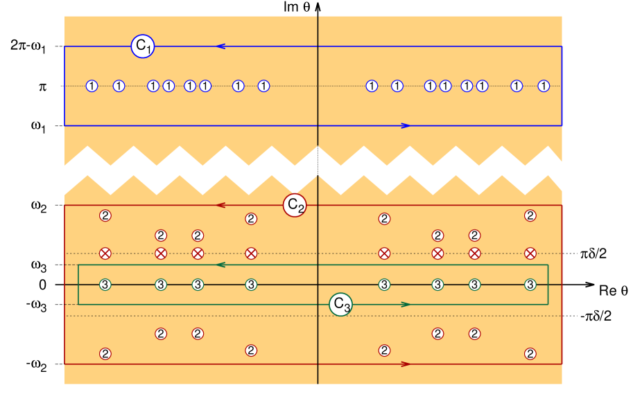
The arrangement of the vacuum roots is illustrated in Fig. 2.
Note that under the “particle-hole” symmetry transformation
| (3.29) |
the sets (I) and (II) transform into one another, whereas the set (III) remains invariant. Obviously the sets (I) and (II) describe the fillings of the vacuum state for and , respectively. The above symmetry proves that the roots , which determine zeroes of , remain unchanged under the transformation (3.29) (this fact has already been mentioned before Eq.(3.19)).
Even though the lattice-type regularization is used here as a technical tool, it would be interesting to construct a lattice model, which actually leads to the BAE presented above. This could provide ideas about a lattice regularization for non-linear sigma models, which so far has not been properly understood. From the point of view of quantum groups such a lattice model could be related to the quantized affine superalgebra or (see [17] for a hidden quantum group structure of the general Fateev model). As noted in [25] it could also be related to algebra -matrices found in [34, 35, 36].
3.3 Scaling limit
In the scaling limit (3.6) the number of BA roots in the central region in Fig. 2 becomes infinite. With the standard Weierstrass regularization the formulae (3.21) and (3.27), with , can be easily turned into convergent infinite products, defining analytic functions , and of the variable , having two essential singularities at and :
| (3.30) |
where the coefficients and are partially constrained by (3.25) and (3.26), but otherwise arbitrary (see a remark after (4.37) below). Obviously, the functions (3.30) can be regarded as vacuum eigenvalues of suitable analogs of Baxter -operators for the BL model.
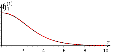
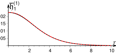
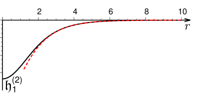
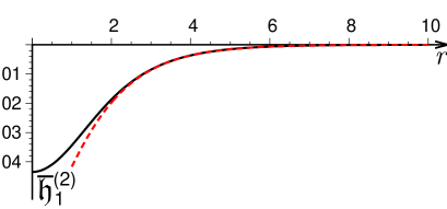
The asymptotic distribution of zeroes of and immediately follows from (3.12) and (Acknowledgment), while for zeroes of (which form 2-strings) one needs to follow the reasonings of [37]. For one obtains
| (3.31) | |||||
where . The zeroes of are located on the real negative axis of , accumulating towards and . The zeroes form 2-strings located just outside the wedge with an acute angle centered around the negative real axis of , where signs “” correspond to lower and upper branches of the wedge. The zeroes of are located at the real axis of (note, that is, actually, a function of ). For small values of the above formulae give a very good approximation to the position of zeroes even for small values of (see Appendix Acknowledgment).
The functions (3.30) satisfy the QFT version of BAE (3.23), (3.28). The later are obtained by rewriting the coefficients there in the form
| (3.32) |
and making the substitution
| (3.33) |
which is reverse to (3.1).
Finally, following the arguments of [31, 38], one can show that in the scaling limit (3.6) an appropriately scaled regularized vacuum energy
| (3.34) |
is expressed in terms of the scaling function (1.3) of the continuous QFT (1.1), where the renormalized field theory twist parameters in (1.2) and their bare counterparts in the BAE (2.28), (2.30) are related as
| (3.35) |
A proof of this statement is presented in Appendix Acknowledgment. Note that another variant of the formula (3.34) for a simple momentum cutoff regularization (rather that the lattice-type regularization of this paper) was presented in [2], see Eq. (5.14) therein. Remarkably, Eq. (3.34) gives reasonably accurate results even for finite values of and , since the main subleading term in the LHS is of the order of .
4 Connection to classical sinh-Gordon equation
The Bethe ansatz equations derived in the previous section allow one to make a connection of the BL model to the classical inverse scattering problem method for the modified sinh-Gordon equation (see [14, 16, 17, 2])
| (4.1) |
for a complex-valued function defined on the Riemann sphere with punctures. Here is an arbitrary constant, while is a function with three singular points located at and ,
| (4.2) |
where
| (4.3) |
Eq.(1.5), given in Introduction, is connected to (4.1) by a simple change of variables
| (4.4) |
and the domain , shown in Fig. 1, is the image of the Riemann sphere with three punctures in the coordinates . However, in this section we prefer to work with Eq. (4.1).
For further references note also that Eq. (4.1) with the choice (4.3) is a particular case of a more general equation [16], where
| (4.5) |
which is connected with the symmetric regime of the Fateev model [23].
4.1 Symmetries of the auxiliary linear problem
The equation (4.1) is the zero-curvature condition for an -valued connection
| (4.6) |
where denotes the complex conjugate of , and is the multiplicative spectral parameter.
Recall that the equations (2.28) and (2.30) are the main ingredients of the coordinate Bethe ansatz solution for the Bukhvostov-Lipatov QFT (1.1). Remarkably, as we shell see below, exactly the same equations are also satisfied by connection coefficients of the linear matrix differential equations
| (4.7) |
associated with modified sinh-Gordon equation (4.1). The required calculations are only slightly different from those related to the Fateev model, considered in details in [17]. Therefore, here we only briefly sketch the main steps of working for the case of the vacuum state of the BL model. In this case the function is a smooth, single-valued complex function without zeroes on a Riemann sphere with three punctures at . The point is assumed to be a regular point on the sphere, where
| (4.8) |
| The asymptotic conditions at the punctures are determined by | |||
| (4.9a) | |||
| and | |||
| (4.9b) | |||
| Note that the above asymptotic conditions are equivalent to (1.6), (1.7) under the substitution (4.4). Below it will be convenient to use parameters related to in (1.2) as,444This is, of course, the same parameters and that already appeared in (3.35), however, in this section they are assumed to be positive and satisfying the relation (4.15). | |||
| (4.10) |
From now on we assume that is a cyclic permutation of . Consider the auxiliary linear problem (4.7). Introduce three matrix solutions
| (4.11) |
normalized by the following asymptotic conditions
| (4.12) |
and
| (4.13) |
for . The constants are defined by
| (4.14) |
The above conditions uniquely determine the solutions provided
| (4.15) |
The connection matrices are defined as
| (4.16) |
They satisfy the obvious relations
| (4.17) |
and
| (4.18) |
Further analysis is based on symmetries of the linear differential equations (4.7). Let
| (4.19) |
be a transformation involving a translation of the independent variable along the contour , going around the point anticlockwise (the variable is translated along complex conjugate contour ), accompanied by the substitution , where
| (4.20) |
Using (4.2) and (4.6) it is easy to check that the substitutions (4.19) leave the system (4.7) unchanged. Therefore they act as linear transformations in the space of solutions. Namely, in the basis they read
| (4.21a) | |||||
| (4.21b) | |||||
| (4.21c) | |||||
where
| (4.22) |
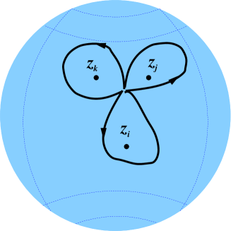
An important property of the linear system (4.7) is that a combined transformation , where is a cyclic permutation of , is equivalent to the identity transformation
| (4.23) |
The proof follows from (4.20) and the fact that is a contractible contour which loops around a regular point on the Riemann sphere, see Fig. 3.
4.2 Functional relations for connection coefficients
The non-trivial functional relation (4.24), complemented with the asymptotic (WKB) analysis of the differential equations (4.7), allows one to completely determine all connection matrices. To within some simple factors, the connection coefficients are meromorphic function of with two essential singularities at and . For the normalization (4.12), (4.13) they could have poles for real negative ’s solving the equations
| (4.25) |
To take this into account it is convenient to introduce a function
| (4.26) | |||||
Note that is a meromorphic function of . It satisfies the functional relation
| (4.27) |
and has the following asymptotics at large real
| (4.28) |
where is the free-boson free energy, which has already appeared in (1.8). The function was originally introduced in [39]. To parameterize the connection coefficients introduce a set of functions , , of the variable , which are analytic everywhere, except the points and . They are defined as
| (4.29) | |||||
where . Note that is, actually, a function of .
Specializing Eq.(4.24) for different choices of the indices and using (4.17) one can obtains a number of important functional relations between ’s (see Appendix Acknowledgment for details)
| (4.30a) | ||||
| (4.30b) | ||||
| (4.30c) | ||||
| (4.30d) | ||||
| where and | ||||
| (4.30e) | ||||
| (4.30f) | ||||
4.3 Asymptotic expansions
The asymptotic behavior of the -functions can be found from the WKB analysis of the linear differential equations (4.7). The required calculations are similar to those of the Fateev model (see Sect. 9 of Ref.[17]). For and , one obtains
| (4.31) | |||||
where and are the same as in (4.10). The leading coefficient is given by
| (4.32) |
where is the Euler constant and . The constant terms (see Eq. (9.19) of Ref.[17])
| (4.33) |
are expressed through the regular parts of the expansions of the solution
| (4.34) |
Further, taking the limit in the results [16] and [17], devoted to the symmetric regime (4.3) of the Fateev model,555Namely, one needs to combine Eqs. (5.27), (6.1) and (9.26) of Ref.[17] with (4.27) of Ref.[2] and then take the limit . one can express the coefficient through the solution of (1.5), satisfying the asymptotic conditions (1.6), (1.7),
| (4.35) |
where the integral is taken over domain shown in Fig.1. The asymptotic expansion of is simply determined by (4.31) and the relation (4.30c).
4.4 Connection to the Bethe ansatz
Remarkably, it turns out that the zeroes of the functions (introduced above as connection coefficients for the differential operators (4.7)) satisfy exactly the same equations (3.23), (3.28), as the zeroes of the functions , arising in the Bethe ansatz description of the vacuum state of the BL model. To make a precise correspondence let us first relate the dimensionless parameter , used in Sects. 1-3, to the parameter , used in (4.1) and further down in this section,
| (4.36) |
Next, recall that the coefficients depend on the parameters defined in (4.10). To indicate this dependence explicitly, we will write these coefficients as . Similarly, the functions , introduced in Sect. 3.3, depend on the twist parameters and , so we will write them as .
Below we are going to establish that
| (4.37) | |||||
where . Recall that here we assume that and are positive, whereas in Sect. 2 and Sect. 3 they were taking both signs. The correspondence is achieved by using the sign variables in RHS of (4.37). Moreover, in writing (4.37) we have assumed a particular choice of normalization factors and the coefficients in (3.30), which so far were at our disposal since they do not affect the position of zeroes of . With this identification it is easy to check the that the functional equations (4.30) imply all the BAE (3.23) and (3.28) in their scaling limit form (recall that the latter is obtained with the help of substitutions (3.32) and (3.33)). For instance, (4.30c) immediately leads the scaling limit of (3.23a) and (3.28b). Similarly, (4.30d) leads to the scaling limit of (3.28a). Finally, setting and in (4.30c) and combining the resulting relations one arrives to (3.23b). Eqs.(3.28c) and (3.28d) are derived in a similar way.
To complete the identification (4.37) one also needs to check that the zeroes of the connection coefficients , determined by the differential equations (4.7), have precisely the same phase assignments (2.36) as the vacuum state zeroes of the BAE. In particular, that the phases are given by consecutive integers containing no “holes” in their distribution. Alternatively, it is enough to prove that and have the same loci of zeroes. We have verified this statement in the small- limit, when the differential equations (4.7) simplify considerably and become ODE’s with explicity known algebraic potentials (see Appendix Acknowledgment). Using asymptotic (WKB) analysis of these ODE’s we show that the corresponding distributions of zeroes precisely match (3.31) in the small- limit. Moreover we have confirmed this coincidence by extensive numerical checks. On this basis we assume (4.37) to hold.
5 Non-linear integral equations
As is well known [40, 41], the BAE can be transformed into NLIE which allow one to accurately calculate vacuum energies as well as eigenvalues of all higher integrals of motion. There are several ways to proceed starting with different sets of BAE discussed after Eq. (3.28). It turns out that the set (III) appears to be most convenient for our purposes. Indeed, in this case the resulting equations admit a regular expansion for small values , which is very convenient for the comparison with perturbation theory calculations of our previous paper [2]. The working is presented in Appendix Acknowledgment. The approach is somewhat similar to that of the regime of the Fateev model, considered in details in Ref.[17]. However, the presence of 2-strings among the vacuum roots makes the considerations rather tedious. As a final result, one obtains the following system of two NLIE:
| (5.1) |
Here , and the kernels are given by the relations
| (5.2) |
with
| (5.3) | |||||
Once the numerical data for are available, any (regularized) sum over the Bethe zeroes can be calculated via fastly converging integral representations (see Appendix Acknowledgment). All information about the vacuum eigenvalues of local and nonlocal integrals of motion is contained in the coefficients of the asymptotic expansions,
| (5.4a) | |||
| and | |||
| (5.4b) | |||
where or , the parameter is defined in (4.36) and the coefficients are given by (4.32). The quantities and are vacuum eigenvalues of the local and nonlocal integrals of motion (for the vacuum state ). The above expansions for are valid for , while for they are valid only for .
The asymptotic expansion of does not contain new coefficients, since it can be obtained by combining (5.4) and (4.30c) (with an account of (4.37)),
| (5.5) | |||||
This expansion is valid for . A similar expansion where are replaced by holds for .
The scaling function (1.3) can be computed by means of the relation
| (5.6) |
which is valid for both choices of the signs , where
| (5.7) |
Moreover, it is worth noting that the lattice-type regularization formula (3.34), written via the integral (D.4), leads precisely to the same expression (5.6). On the other hand, in view of the identification (4.37), one can compare terms of the expansions (4.31) and (5.4). Then, taking into account (4.28), one arrives to the alternative expression (1.4) for the scaling function in terms of solutions of the classical sinh-Gordon equation (1.5), stated in Introduction.
As demonstrated in [2] the exact formula (5.6) is in a perfect agreement with the results of renormalized perturbation theory and conformal perturbation theory. It is possible to show that (5.6) implies the following large- asymptotics,
where is the modified Bessel function, and .
Besides the vacuum energies the non-linear integral equations allows one to determine the vacuum eigenvalues of all higher Integral of Motions (IM). In particular, the vacuum eigenvalues of the local IM, for , are given by the formula generalizing (5.6),
| (5.9) |
Some details concerning small- and large- behavior of , along with numerical data for and can be found in Appendix Acknowledgment.
Among the nonlocal IM the special rle is played by the so-called reflection operators [16]. Their vacuum eigenvalues are related to the scaling function [16],
| (5.10) |
and can be calculated through the solution of the system (5.1):
| (5.11) |
On the other hand, taking into account (4.37) and comparing the constant terms in the expansions (4.31) and (5.4), one arrives to an alternative expression (4.35) of in terms of the regular part of the solution of the modified sinh-Gordon equation (4.1), (4.9).666 The expression (4.35) can be rewritten in terms of the function , satisfying (1.5) and (1.6), (5.12) where and .
The large- behavior of follows immediately from Eqs.(5), (5.10):
| (5.13) | |||||
where
| (5.14) |
Using the small- asymptotic expansion
| (5.15) |
where a few first coefficients was calculated in [2] (see Eq.(2.19) therein) one also finds
| (5.16) |
The first term in the RHS reads explicitly [16]
| (5.17) |
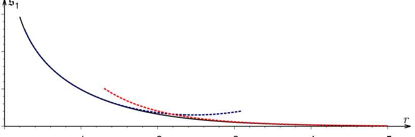
In Fig. 4 the numerical results for are compared against the large- and small- asymptotic formulae (5.13) and (5.16).
Finally, there is an infinite set of non-local IM, whose vacuum eigenvalues are given by the relations:
| (5.18) | |||||
Some further details can be found in Appendix Acknowledgment.
6 Summary
This work completes our study of the Bukhvostov-Lipatov (BL) model, started in [2]. Besides its applications to the instanton calculus in the non-linear sigma model, the BL model provides an ideal testground to developing new and refining existing methods for integrable QFT’s. Our attention was mostly devoted to calculation of the scaling function (1.3) (which is simply related to the so-called effective central charge) of the BL model in a finite volume and the quasiperiodic boundary conditions. The scaling function was computed in a variety of different ways. For the readers’ convenience let us briefly summarize our main results below:
-
(i)
the conformal perturbation theory for a few first terms in the small- expansion of the scaling function;
-
(ii)
the renormalized Matsubara perturbation theory (recall that we consider the finite-volume theory) for two non-trivial orders of the expansion of the scaling function in powers of the coupling constant;
-
(iii)
an exact formula for the scaling function in terms of different sets of non-linear integral equations (NLIE) derived from the Bethe ansatz and functional relations;
-
(iv)
an exact formula for the scaling function in terms of a special solution of the classical sinh-Gordon equation, based on the ODE/IQFT correspondence and the classical inverse scattering transform;
-
(v)
renormalization of the coordinate Bethe ansatz results for the scaling function both with the lattice-type regularization and the simple momentum cut-off.
Remarkably, all the above approaches perfectly agree to each other. This allowed us to establish the ODE/IQFT correspondence between the quantum Bukhvostov-Lipatov model and the classical sinh-Gordon equation. Note that this correspondence has recently been extended to the strong coupling regime of the BL model with [42]. In this case it provides a dual description of the 2D sausage [24], which includes the -sigma model when .
It would be interesting to further develop the “quantum-classical” duality, in particular, to explore its possible connections to the duality between quantum and classical systems with a finite number of degrees of freedom, studied in [43].
Acknowledgment
The authors thank R. Baxter, M. Batchelor, G. Dunne, A. Gorsky, M. Jimbo, I. Krichever, J-M. Maillet, A. Marshakov, A. Pogrebkov and F. Smirnov for fruitful discussions.
Research of S.L. was supported by the NSF under grant number NSF-PHY-1404056.
Appendix A.
Here we present details of derivation of the individual functional relations (4.30) for the connection coefficients, starting from the main functional relation (4.24) for the connection matrices,
| (A.1) |
Take and express through and in two different ways: from the main relation (A.1)
and from the simple properties (4.17) of the connection matrices,
| (A.2) |
This system contains both and . Choose in both equations, fix a particular sign , and then exclude among the above two equations. In this way one obtains
which is equivalent to (4.30d) upon the substitution (4.29).
Next, take main relation (A.1) with and express therein in terms of product of and using relation similar to (A.2) with shifted spectral parameter . It follows then
Setting and combining like terms one obtains the relation
which is equivalent to (4.30a) upon the substitution (4.29). One can repeat the above steps excluding from (A.1). This leads to the relation (4.30b).
Finally, express from (A.1) as
and from (A.2) (with shifted spectral parameter)
Then the product can be excluded from the above equations, leading to
which is equivalent to (4.30c) upon the substitution (4.29).
Appendix B. Conformal field theory limit
To understand properties of the connection coefficients it is instructive to first consider the small-distance limit . The linear equations (4.7) can be reformulated as second order ordinary differential equations. For example, making the substitution
| (B.1) |
in the first equation of (4.7), one obtains
| (B.2) |
Let denote the bases of solutions of this second order equation, which under the substitution (B.1) precisely correspond to the solutions , defined by (4.12), (4.13). Then the connection problem (4.16) can be rewritten as
where . Note also, that (B.1) implies
| (B.3) |
where denotes the usual Wronskian.
Consider now the limit when , but the product is kept fixed. In this limit the variable completely decouples from (B.2) and the potential term there simplifies
| (B.4) |
where . The basis solutions, corresponding to (4.12) and (4.13), become
where the constants should be computed at , while is kept finite.
Further, by a change of variables
the differential equation (B.2), (B.4) can be cast into a form more suitable for analytical and numerical analysis,
| (B.5) |
The branch cuts of the power function are chosen to be on the lines, where is real and negative. Therefore, there are no branch cuts in the -plane, when . The symmetry transformations and defined in (4.19) above act as follows:
Introduce two bases of solutions and , which are uniquely defined by their asymptotic behavior
and symmetry transformation properties
Note that . With these definitions introduce the functions
| (B.6) |
defined as Wronskian determinants. Further, interchanging and in (Acknowledgment) and proceeding as above one defines another pair of connection coefficients
| (B.7) |
which are obtained from by interchanging and and the negation of .
Yet another form of (B.5)
| (B.8) |
is obtained by the substitution
which includes a phase rotation of the spectral parameter . Similarly to the above, introduce the solutions and defined by their asymptotics
and symmetry properties
Now define the functions
| (B.9) |
From the standard analysis of the differential equation (B.5) it is easy to see that the functions are entire functions of the complex variable , while the are entire functions of the variable . The asymptotic expansion of at large is given by
| (B.10) |
where or ,
as and . A few first expansion coefficients is known explicitly, in particular,
where stands for Euler constant, and . Moreover,
The coefficients are entire functions of the complex variable . Their asymptotic expansion at large is given by
| (B.11) |
and as and
| Zeroes of | ||
|---|---|---|
| (numerical) | (asymptotic formula (B.12)) | |
| 1 | -0.32118644 | -0.28671875 |
| 2 | -0.78656554 | -0.78671875 |
| 3 | -1.28902812 | -1.28671875 |
| 4 | -1.78780916 | -1.78671875 |
| 5 | -2.28754568 | -2.28671875 |
| Zeroes of | ||
| (numerical) | (asymptotic formula (B.12)) | |
| 1 | -0.25404467 | -0.21328125 |
| 2 | -0.71063637 | -0.71328125 |
| 3 | -1.21516013 | -1.21328125 |
| 4 | -1.71396329 | -1.71328125 |
| 5 | -2.21383761 | -2.21328125 |
| Zeroes of | ||
|---|---|---|
| (numerical) | (asymptotic formula (B.13)) | |
| 1 | -0.41729701-0.37695011 i | -0.44259358-0.39285900 i |
| 2 | -1.12935605-0.82780500 i | -1.15306097-0.84640446 i |
| 3 | -1.83960684-1.28084953 i | -1.86352835-1.29994992 i |
| 4 | -2.54998314-1.73418285 i | -2.57399573-1.75349537 i |
| 5 | -3.28446342-2.20704109 i | -3.28446311-2.20704083 i |
| 6 | -3.99491662-2.66056721 i | -3.99493049-2.66058629 i |
| 7 | -4.70539788-3.11413172 i | -4.70539787-3.11413175 i |
| 8 | -5.41586525-3.56767720 i | -5.41586525-3.56767720 i |
| 9 | -6.12633265-4.02122266 i | -6.12633263-4.02122266 i |
| Zeroes of | ||
|---|---|---|
| (numerical) | (asymptotic formula (B.14)) | |
| 1 | 0.58940086 i | 0.58444921 i |
| 2 | 1.42941557 i | 1.42734148 i |
| 3 | 2.27132015 i | 2.27023375 i |
| 4 | 3.11381245 i | 3.11312602 i |
| 5 | 3.95650092 i | 3.95601829 i |
| 6 | 4.79927351 i | 4.79891057 i |
| 7 | 5.64208861 i | 5.64180284 i |
| 8 | 6.48492773 i | 6.48469511 i |
| 9 | 7.32778156 i | 7.32758738 i |
| 10 | 8.17064498 i | 8.17047965 i |
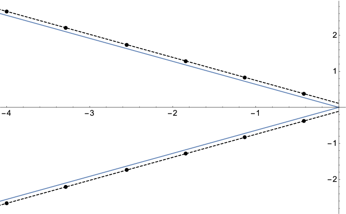
Let denote the zeroes of . For sufficiently small and large they are distributed as follows:
-
•
the zeroes of are located on the real negative axis of variable
(B.12) -
•
the zeroes of combine into complex conjugate pairs in the left half-plane , located just outside the wedge with an acute angle centered around the negative real axis of (see Fig. 5)
(B.13) -
•
the zeroes of are simple, real and negative,
(B.14)
The above asymptotic formulae are in a very good agreement with the numerical values of the zeroes obtained from a direct solution of the differential equation (B.5), (B.8) even for small values of (see Tables 1,2,3).
Appendix C. Derivation of non-linear integral equations
As noted above one can derive several different, but equivalent variants of the non-linear integral equations, starting with different BAE. Below we will use the three equations (3.23a), (3.28a) and (3.28b). Introduce two functions
| (C.1) | |||||
which appear in the RHS’s of (3.23a) and (3.28a). The other relevant notations are given in (3.3), (3.24), (3.21) and (3.27). These functions are periodic with the period
and possess the following symmetry
under the complex conjugation. Note that in the strip the function has following poles and zeroes,
| (C.2a) | |||||
| (C.2b) | |||||
Taking the logarithms, one obtains
| (C.3a) | ||||
| (C.3b) | ||||
where and are defined in (3.1) and (2.33). The indices and run over the values , with being an even integer. The (complex) numbers , and stand for the zeroes of the functions , and , as defined by (3.21), (3.27). With these notations BAE (3.23a), (3.28a) and (3.28b) take the form
Fig. 6 shows the contours , and enclosing zeroes of , and , respectively. The horizontal segments of these contours go along the lines , , with the positive constants , and , satisfying the inequalities
| (C.4) |
where
is the maximal deviation of the roots from the line . The second inequality in (C.4) ensures that the contour in Fig. 6 encloses all zeroes of .
Next, the sum in (C.3a) and the first sum in (C.3b) can be easily written as contour integrals, for instance
| (C.5a) | |||
| and similarly | |||
| (C.5b) | |||
The handling of the second sum in (C.3b) is slightly more complicated, since the contour (which is enclosing the zeroes of ), also surrounds (unwanted) poles of located on the line . Taking this into account one obtains
| (C.6) |
Further considerations follow the standard way [40, 41] of deriving the non-linear integral equations. Substitute (C.5) back into (C.3). Integrating by parts, stretching the contours towards both infinities along the real axis of and introducing the pseudo-energies
| (C.7) |
one obtains
| (C.8) | |||
where ,
and
The integral operators are conveniently defined by their Fourier transforms. We use the following general convention
| (C.9) |
The matrix elements then take the form
where
and
For completeness we present also the Fourier transform of the source term in (C.8)
for which one should use the principal value integral in (C.9). Multiplying both sides of (C.8) by the inverse of the matrix integral operator , one obtains
| (C.10) | |||||
where the Fourier transform of the kernel is given by
with
For the source terms in (C.10) one obtains
and
where the functions and were already defined in (3.13).
Equation (C.10) can be considerably simplified thanks to some additional symmetries. Indeed, using the Fourier transform of the integral operator one can see that all the dependence on the functions in RHS of (C.10) reduces to the integrals
| (C.11) |
where for any finite and . Then using the definitions (C.7) and the fact that the function does not have poles or zeroes (C.2) in the strip one can shift the integration contours in (C.11) to prove that
| (C.12) |
Thus, one of the functions or can be excluded from (C.10).
Consider now the scaling limit (3.6) of (C.10). For the central region one needs to make the substitution
for , while the rest of (C.10) remains intact. Next, using the symmetry (C.12) to exclude , redenoting and , and then choosing and to be infinitesimally small, one arrives to Eq. (5.1), given in the main text.
Appendix D. Integral representations for sums over the Bethe roots
Once the non-linear integral equations (C.10) are solved, every sum over the vacuum Bethe roots can be effectively computed via exact integral representations, considered below. The technique works equally well both for finite values of (when the number of Bethe roots is finite) as well as in the scaling limit (when and (C.10) is replaced by its field theory analog (5.1)).
Let us start with the case of finite . Consider, for instance, the product formulae (3.21) and (3.27). With an account of (C.10) they can be converted into integral representations
| (D.1) | |||||
where , ,
| (D.2) |
The Fourier transform of the kernel is defined by (C.9) (but with the principal value integral) where
| (D.3) | |||||
The derivation is standard and very much similar to that of the equation (C.10) itself. The only complication is that one needs to systematically take into account the fact that summing over the zeroes of with integrals over the contour in Fig. 6 (similarly to (C.6)) contains extra contributions determined by the zeroes of . Moreover, the function was excluded from the RHS of (D.1) in favor of of by virtue of (C.12). We have presented the intermediate formulae (Acknowledgment) to guide the reader through this tedious derivation. From (Acknowledgment) one obtains
Similar representations can be obtained for the two expressions for the energy (3.5), when the vacuum state is filled with real roots (1-strings) and complex roots (2-strings), respectively,
Proceeding as above, one obtains for
| (D.4) | |||||
where
In particular for the difference between LHS and RHS of (3.20) one gets
which is zero, since vanishes, as stated in (C.2).
Scaling limit. Consider now the scaling limit (3.6). Then (D.1) can be used to obtain integral representations for the -functions (3.30) for the BL model. The only modification is that for one needs to add to the RHS of (D.1) the entire functions , that appear in (3.30). Assume that . Then for the leading terms in (D.1) one obtains in the limit (3.6),
where
The undetermined coefficients are fixed by the requirement that the functions (3.30) satisfy the functional relation (4.30c) (upon the identification (4.37)). The integral representations for obtained in this way, lead to the asymptotic expansions (5.4), with the coefficients given by (5.9) and (5.18).
Finally, note that in the scaling limit (3.6) formula (D.4) leads precisely to (3.34). First, let us split the integration in (D.4) into two regions, where and . Then, it is not difficult to see that the contribution of the first integral to the LHS of (3.34) exactly equals to (in the form (5.6)), while the second integral gives the term “” in the RHS of (3.34).
Appendix E. Small and large- asymptotics of IM
Here we collect some facts concerning the vacuum eigenvalues of integral of motions in the BL model. The local IM are normalized in such a way that
| (E.1) |
Here are certain polynomials of two variables of degree , such that
where is the Pochhammer symbol and dots stand for monomials with degree lower than . The polynomial and read explicitly [44]:777The polynomials from Ref.[44] are related to as
| (E.2) | |||||
and
| (E.3) |
The vacuum eigenvalues of local IM (5.9) can be written in the form
| (E.4) |
where
and, as ,
| (E.5) |
with
and
The relations (E.4) are valid for any choice of the sign and . Also notice that for the non interacting case
and .
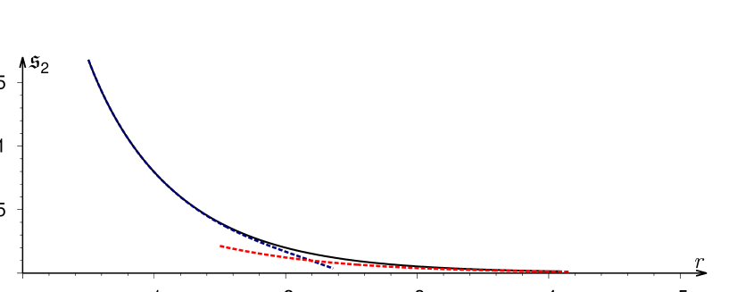
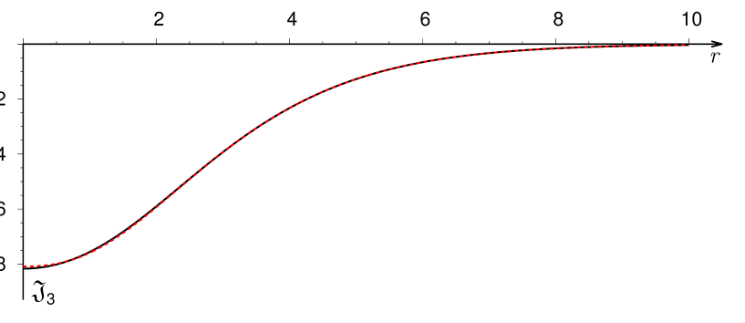
In Fig. 7, the numerical data for vacuum eigenvalues of the first local IM are compared against the large- approximation (E.4), (E.5).
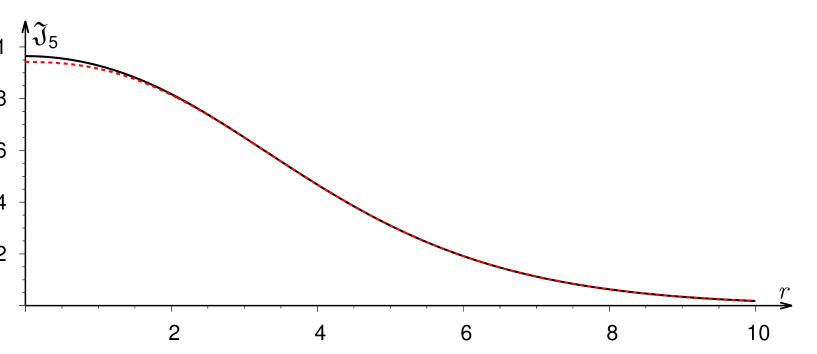
Similarly to the formula (E.4), the vacuum eigenvalues of nonlocal IM (5.18) are expressed in terms of the -function (E.5):
| (E.6) |
This gives the corresponding large- asymptotics (see Fig. 8). In the small- limit one has
| (E.7) |
An integral representation for these limiting values where discussed in Ref.[17]. Using the results of this work, it is possible to show that
| (E.8) |
References
- [1] A. P. Bukhvostov and L. N. Lipatov, “Instanton – anti-instanton interaction in the nonlinear -model and an exactly soluble fermion theory”, Nucl. Phys. B180 (1981) 116.
- [2] V. V. Bazhanov, S. L. Lukyanov and B. A. Runov, “Vacuum energy of the Bukhvostov-Lipatov model”, Nucl. Phys. B911 (2016) 863–889, arXiv:1607.04839 [hep-th].
- [3] A. A. Belavin and A. M. Polyakov, “Metastable states of two-dimensional isotropic ferromagnets”, JETP Lett. 22 (1975) 245–248. [Pisma Zh. Eksp. Teor. Fiz. 22, 503 (1975)].
- [4] V. A. Fateev, I. V. Frolov and A. S. Schwarz, “Quantum fluctuations of instantons in the nonlinear sigma model”, Nucl. Phys. B154 (1979) 1–20.
- [5] A. Voros, “Exact quantization condition for anharmonic oscillators (in one dimension)”, J. Phys. A 27 no. 13, (1994) 4653–4661.
- [6] P. Dorey and R. Tateo, “Anharmonic oscillators, the thermodynamic Bethe ansatz and nonlinear integral equations”, J. Phys. A 32 no. 38, (1999) L419–L425. [arXiv:hep-th/9812211].
- [7] V. V. Bazhanov, S. L. Lukyanov and A. B. Zamolodchikov, “Spectral determinants for Schrodinger equation and operators of conformal field theory”, J. Statist. Phys. 102 (2001) 567–576, arXiv:hep-th/9812247.
- [8] J. Suzuki, “Functional relations in Stokes multipliers: Fun with potential”, J. Statist. Phys. 102 (2001) 1029–1047, arXiv:quant-ph/0003066.
- [9] V. V. Bazhanov, A. N. Hibberd and S. M. Khoroshkin, “Integrable structure of conformal field theory, quantum Boussinesq theory and boundary affine Toda theory”, Nucl. Phys. B622 (2002) 475–547, arXiv:hep-th/0105177.
- [10] V. V. Bazhanov, S. L. Lukyanov and A. B. Zamolodchikov, “Higher level eigenvalues of operators and Schroedinger equation”, Adv. Theor. Math. Phys. 7 no. 4, (2003) 711–725, arXiv:hep-th/0307108.
- [11] D. Fioravanti, “Geometrical loci and CFTs via the Virasoro symmetry of the mKdV-SG hierarchy: An Excursus”, Phys. Lett. B609 (2005) 173–179, arXiv:hep-th/0408079.
- [12] P. Dorey, C. Dunning, D. Masoero, J. Suzuki and R. Tateo, “Pseudo-differential equations, and the Bethe ansatz for the classical Lie algebras”, Nucl. Phys. B772 (2007) 249–289, arXiv:hep-th/0612298.
- [13] B. Feigin and E. Frenkel, “Quantization of soliton systems and Langlands duality”, arXiv:0705.2486 [math.QA].
- [14] S. L. Lukyanov and A. B. Zamolodchikov, “Quantum Sine(h)-Gordon Model and Classical Integrable Equations”, JHEP 07 (2010) 008, arXiv:1003.5333 [math-ph].
- [15] P. Dorey, S. Faldella, S. Negro and R. Tateo, “The Bethe Ansatz and the Tzitzeica-Bullough-Dodd equation”, Phil. Trans. Roy. Soc. Lond. A371 (2013) 20120052, arXiv:1209.5517 [math-ph].
- [16] S. L. Lukyanov, “ODE/IM correspondence for the Fateev model”, JHEP 12 (2013) 012, arXiv:1303.2566 [hep-th].
- [17] V. V. Bazhanov and S. L. Lukyanov, “Integrable structure of Quantum Field Theory: Classical flat connections versus quantum stationary states”, JHEP 09 (2014) 147, arXiv:1310.4390 [hep-th].
- [18] D. Masoero, A. Raimondo and D. Valeri, “Bethe Ansatz and the Spectral Theory of Affine Lie Algebra-Valued Connections I. The simply-laced Case”, Commun. Math. Phys. 344 no. 3, (2016) 719–750, arXiv:1501.07421 [math-ph].
- [19] K. Ito and C. Locke, “ODE/IM correspondence and Bethe ansatz for affine Toda field equations”, Nucl. Phys. B896 (2015) 763–778, arXiv:1502.00906 [hep-th].
- [20] L. D. Faddeev, E. K. Sklyanin and L. A. Takhtajan, “The quantum inverse problem method. 1”, Theor. Math. Phys. 40 (1980) 688.
- [21] L. D. Faddeev and L. A. Takhtajan, Hamiltonian Methods in the Theory of Solitons. Springer-Verlag, Berlin, 1987.
- [22] V. V. Bazhanov, G. A. Kotousov and S. L. Lukyanov, “Winding vacuum energies in a deformed sigma model”, Nucl. Phys. B889 (2014) 817–826, arXiv:1409.0449 [hep-th].
- [23] V. A. Fateev, “The sigma model (dual) representation for a two-parameter family of integrable quantum field theories”, Nucl. Phys. B473 (1996) 509–538.
- [24] V. A. Fateev, E. Onofri and A. B. Zamolodchikov, “The sausage model (integrable deformations of sigma model)”, Nucl. Phys. B406 (1993) 521–565.
- [25] H. Saleur, “The long delayed solution of the Bukhvostov-Lipatov model”, J. Phys. A32 (1999) L207, arXiv:hep-th/9811023.
- [26] R. J. Baxter, Exactly solved models in statistical mechanics. Academic, London, 1982.
- [27] E. H. Lieb, “Exact solution of the problem of the entropy of two-dimensional ice”, Phys. Rev. Lett. 18 no. 17, (Apr, 1967) 692–694.
- [28] R. J. Baxter, “Generalized ferroelectric model on a square lattice”, Stud. Appl. Math. 1 (1971) 51–69.
- [29] R. J. Baxter, Exactly Solved Models in Statistical Mechanics. Academic, London, 1982.
- [30] L. A. Takhtajan and L. D. Faddeev, “The quantum method for the inverse problem and the Heisenberg model”, Uspekhi Mat. Nauk 34(5) no. 5, (1979) 13–63. (English translation: Russian Math. Surveys 34(5) (1979) 11–68).
- [31] C. Destri and H. J. De Vega, “Unified approach to thermodynamic Bethe Ansatz and finite size corrections for lattice models and field theories”, Nucl. Phys. B438 (1995) 413–454, arXiv:hep-th/9407117.
- [32] F. H. L. Essler, V. E. Korepin and K. Schoutens, “Exact solution of an electronic model of superconductivity in (1+1)-dimensions. 1.”, Int. J. Mod. Phys. B8 (1994) 3205, arXiv:cond-mat/921100.
- [33] P. P. Kulish, “Integrable graded magnets”, J. Sov. Math. 35 (1986) 2648–2662. [Zap. Nauchn. Semin.145,140(1985)].
- [34] T. Deguchi, A. Fujii and K. Ito, “Quantum superalgebra ”, Phys. Lett. B 238 no. 2, (1990) 242 – 246.
- [35] M. D. Gould, J. R. Links, Y.-Z. Zhang and I. Tsohantjis, “Twisted quantum affine superalgebra , invariant -matrices and a new integrable electronic model”, J. Phys. A 30 (1997) 4313.
- [36] M. J. Martins and P. B. Ramos, “On the solution of a supersymmetric model of correlated electrons”, Phys. Rev. B56 (1997) 6376, arXiv:hep-th/9704152.
- [37] H. J. de Vega and F. Woynarovich, “Solution of the Bethe Ansatz Equations with Complex Roots for Finite Size: The Spin Isotropic and Anisotropic Chains”, J. Phys. A23 (1990) 1613.
- [38] S. L. Lukyanov, “Critical values of the Yang-Yang functional in the quantum sine-Gordon model”, Nucl. Phys. B853 (2011) 475–507, arXiv:1105.2836 [hep-th].
- [39] S. L. Lukyanov, “Finite temperature expectation values of local fields in the sinh-Gordon model”, Nucl. Phys. B612 (2001) 391–412, arXiv:hep-th/0005027.
- [40] A. Klümper, M. T. Batchelor and P. A. Pearce, “Central charges of the 6- and 19-vertex models with twisted boundary conditions”, J. Phys. A. 24 (1991) 3111–3133.
- [41] C. Destri and H. J. de Vega, “New thermodynamic Bethe ansatz equations without strings”, Phys. Rev. Lett. 69 (1992) 2313–2317.
- [42] V. V. Bazhanov, G. A. Kotousov and S. L. Lukyanov, “Quantum transfer-matrices for the sausage model”, arXiv:1706.09941 [hep-th].
- [43] A. Gorsky, A. Zabrodin and A. Zotov, “Spectrum of Quantum Transfer Matrices via Classical Many-Body Systems”, JHEP 01 (2014) 070, arXiv:1310.6958 [hep-th].
- [44] S. L. Lukyanov, E. S. Vitchev and A. B. Zamolodchikov, “Integrable model of boundary interaction: The Paperclip”, Nucl. Phys. B683 (2004) 423–454, arXiv:hep-th/0312168.