Survival behavior in the cyclic Lotka-Volterra model with a randomly switching reaction rate
Abstract
We study the influence of a randomly switching reproduction-predation rate on the survival behavior of the non-spatial cyclic Lotka-Volterra model, also known as the zero-sum rock-paper-scissors game, used to metaphorically describe the cyclic competition between three species. In large and finite populations, demographic fluctuations (internal noise) drive two species to extinction in a finite time, while the species with the smallest reproduction-predation rate is the most likely to be the surviving one (law of the weakest). Here, we model environmental (external) noise by assuming that the reproduction-predation rate of the strongest species (the fastest to reproduce/predate) in a given static environment randomly switches between two values corresponding to more and less favorable external conditions. We study the joint effect of environmental and demographic noise on the species survival probabilities and on the mean extinction time. In particular, we investigate whether the survival probabilities follow the law of the weakest and analyze their dependence on the external noise intensity and switching rate. Remarkably, when, on average, there is a finite number of switches prior to extinction, the survival probability of the predator of the species whose reaction rate switches typically varies non-monotonically with the external noise intensity (with optimal survival about a critical noise strength). We also outline the relationship with the case where all reaction rates switch on markedly different time scales.
pacs:
05.40.-a, 87.23.Kg, 02.50.Ey, 87.23.-nI Introduction
Ecosystems consist of a large number of interacting species and the competition for resources affects their survival and reproduction probability May73 ; Hubbell . Studying the mechanisms allowing the maintenance of species diversity and what affects their coexistence is therefore a question of great interest and a major scientific challenge Pennisi05 . In this context, the birth and death events arising in a population cause demographic fluctuations in the number of organisms VanKampen ; Gardiner . This internal noise is important because it can ultimately lead to species extinction Hubbell ; Kimura ; Ewens ; RMF06 ; Berr09 ; Frey10 . For instance, experiments on colicinogenic microbial communities have demonstrated that cyclic, rock-paper-scissors-like, competition leads to intriguing behavior Kerr02 : when the population is well mixed in flasks, the strain that is resistant to the poison (colicin) is the only one to survive after a brief transient; whereas all species coexist for a long time when the same population competes on a plate (Petri dish). It has also been found that rock-paper-scissors-type competition characterizes the dynamics of certain lizard communities and coral reef invertebrates Sinervo96 ; Jackson . These observations have motivated a large body of work, with many theoretical studies focusing on the circumstances under which cyclic competition of rock-paper-scissors type yield species coexistence, see, e.g., MayLeonard ; Maynard ; RMF06 ; Berr09 ; RMF07a ; RMF07b ; RMF08 ; He10 ; Mobilia10 ; He11 ; JPAtopical ; cycl-rev . In particular, it has been shown that species migration can both help promote and jeopardize biodiversity in these systems Kerr06 ; RMF07a ; RMF07b ; RMF08 ; JPAtopical ; cycl-rev , and can lead to the formation of fascinating spiraling patterns, see, e.g., Refs. RMF07a ; RMF07b ; RMF08 ; Matti08 ; RF08 ; JPAtopical ; cycl-rev ; BS14 ; SMR13 ; SMR14 ; MRS16 ; Rucklidge17 . The question of the species survival (or fixation) probability is also of considerable interest both from a theoretical and practical viewpoint. For example, in the flask experiments of Ref. Kerr02 , the surviving strain is always the one that is resistant to the colicin. In order to understand this and related puzzling results, the survival behavior of the cyclic Lotka-Volterra model (CLV), in which three species are in cyclic competition according to zero-sum rock-paper-scissors interactions, see, e.g., Refs. Hofbauer ; Nowak ; Broom ; Maynard ; Ifti03 ; Frean01 ; RMF06 ; RMF08b ; Berr09 ; Tainaka89 ; Tainaka94 ; Tainaka93 ; He10 ; Ni10 ; Venkat10 ; Mitarai16 ; Frachebourg96 ; Szabo02 ; Perc07 ; Dob12 , has been investigated. It has been shown that due to demographic fluctuations the CLV dynamics necessarily ends up in one of the absorbing states where only one of the species survives Ifti03 ; Frean01 ; RMF06 ; RMF08b ; Berr09 ; Dob12 . Furthermore, the authors of Ref. Berr09 showed that, in a large and well-mixed population, the species with the lowest reproduction-predation rate (“weakest species”) is the most likely to be the surviving one, with a probability that approaches one in large populations, a result dubbed as the “law of the weakest” (see also Refs. Frean01 ; Tainaka93 for other formulations of this “law”).
In addition to demographic noise, populations are subject to ever-changing environmental conditions which influence their reproduction and survival probability. For instance, variation in the abundance of nutrients, or changes in external factors (e.g., light, pH, temperature, moisture, humidity) can influence the evolution of a population Levins ; Schaffer ; Morley83 ; Fux05 . The variation of environmental factors is often modeled as external noise by assuming that the reproduction or predation rate of some species fluctuates in time Karlin74 ; Chesson81 ; Balaban04 ; Kussell05 ; Beaumont09 ; Acer08 ; Dobramysl13 ; Assaf12 ; Assaf13 ; Ashcroft14 ; Melbinger15 ; Danino16 ; Thattai01 ; Kussell05b ; Hufton16 ; Hidalgo17 ; Xue17 . The population is thus subject to demographic (internal) noise and environmental randomness (external noise). A question of great relevance is thus to understand how populations evolve under the joint effect of internal and external noise. In fact, while it is well known that internal noise can lead to species extinction it is unclear how external noise influences the species survival probabilities and the mean extinction time. For instance, in Ref. Assaf13 the fixation probability has been found to vary non-monotonically with the external noise’s correlation time whereas in Refs. KEM17 ; KEM18 the probability either increases or decreases with it.
For the sake of completeness, we mention that another source of randomness arises when the dynamics takes place on complex networks with irregular connectivity. For instance, the CLV dynamics on small-world networks is characterized by limit cycles and noisy oscillations of the species densities, see, e.g., Refs. Sato ; Szabo ; Szolnoki ; Tainaka94 .
Here, we consider the non-spatial CLV and focus on the interplay between demographic fluctuations and environmental noise. Most of the theoretical studies on the joint influence of internal and external noise, have effectively focused on two-species systems or non-interacting populations Karlin74 ; Thattai01 ; Kussell05b ; Assaf12 ; Assaf13 ; Ashcroft14 ; Melbinger15 ; Danino16 ; Hufton16 ; Hidalgo17 ; Xue17 ; KEM17 ; Spalding17 ; Danino17 , often with white external noise, see, e.g., Refs. May73 ; Karlin74 ; Melbinger15 . Here, we study how internal and external dichotomous noise, a simple colored noise with realistic finite correlation time HL06 ; Bena06 , jointly influence the mean extinction time and survival probabilities of the three species of the CLV. For this, we assume that the reproduction-predation rate of the fastest species to reproduce and predate in a static environment (strongest species) switches between two values corresponding to more and less favorable external conditions Balaban04 ; Acer08 . By combining the properties of the classical CLV with those of the underlying “piecewise-deterministic Markov process” PDMP1 ; PDMP2 , see Sec. III, we study how the intensity and switching rate of the environmental noise affects the species survival behavior.
The cyclic Lotka-Volterra model with dichotomous noise (CLVDN) is defined in the next section, where its mean-field and survival properties in the absence of external noise are reviewed. Section III is dedicated to the description of the CLVDN in terms of the piecewise deterministic Markov process. The survival probabilities and mean extinction time are discussed in Sec. IV and comprehensively summarized in Section V. Our conclusions are presented in Sections VI. In the Appendices, we give some technical details and outline how our results shed light on the scenario where the three reaction rates randomly switch on markedly different time scales.
II The Cyclic Lotka-Volterra Model with dichotomous noise (CLVDN)
We consider a well-mixed population (no spatial structure) of size containing three species. The population consists of individuals of species , of type and individuals of species . While the population size is constant, , its composition changes in time due to the cyclic competition between all species: dominates over which dominates over , which in turns out-competes . While there are different forms of cyclic dominance, here we model the cyclic competition in terms of the cyclic Lotka-Volterra (CLV) according to the reaction scheme Hofbauer ; Nowak ; Broom ; Maynard ; Ifti03 ; Frean01 ; RMF06 ; RMF08b ; Berr09 ; Tainaka89 ; Tainaka93 ; Tainaka94 ; He10 ; Ni10 ; Venkat10 ; Mitarai16 ; Frachebourg96 ; Szabo02 ; Perc07 ; Dob12 :
| (1) | |||||
Accordingly, when and interact, kills and instantly replaces it by one of its copy (offspring) with a reproduction-predation rate . Similarly, and are the reaction rates associated with the other reproduction-predation reactions. This model corresponds to the celebrated (zero-sum) rock-paper-scissors game Maynard ; Hofbauer ; Nowak ; Broom . Other popular choices to model cyclic dominance are the May-Leonard model MayLeonard and the combination of the latter and CLV, see, e.g., Refs. RMF07 ; RMF07b ; RMF08 ; RF08 ; JPAtopical ; cycl-rev ; SMR13 ; SMR14 ; MRS16 .
In this work, we are interested in the influence of environmental randomness on the dynamics of cyclic dominance. As a simple form of external noise, in all Sections (except Sec. III), we assume that species is the strongest in a static environment, where , and that its reproduction-predation rate fluctuates with the environment, i.e. (see Eq. (3) below). This can be interpreted as the situation where species , that is the most relentless to predate and reproduce, is also the most exposed to changes in exogenous factors. Here, these are assumed to be responsible for the switch with rate of between the values (in an environment more favorable to ) and (in conditions less favorable to ) , while the effect of the external factors on and is assumed to be negligible (but see also Appendix A).
As in other contexts, see, e.g., Refs. Thattai01 ; Kussell05b ; Ashcroft14 ; Hufton16 ; Hidalgo17 ; Xue17 ; KEM17 , the environmental colored noise is simply modeled as a continuous-time dichotomous Markov noise (DN) with zero mean, ( denotes the ensemble average) and autocorrelation function , where is the finite correlation time HL06 ; Bena06 . We therefore study the CLV subject to DN, a model henceforth labeled CLVDN, obtained by supplementing the scheme (II) with the symmetric dichotomous colored noise corresponding to the switching reaction
| (2) |
such that the reaction occurs with the time-fluctuating rate , with
| (3) |
where is the intensity of the environmental noise. In this setting, the environmental state is more favorable to species than the static environment (), while it is less favorable when Balaban04 ; Acer08 . Clearly, corresponds to the CLV in the absence of external noise, whereas we notice that when , or with a probability , and in this case also there is an external source of randomness when . It is worth noting that the DN (2) has the same autocorrelation function as an Ornstein-Uhlenbeck process, which is another common type of external noise, see e.g. Assaf12 ; Assaf13 , with continuous environmental states 111 The Ornstein-Uhlenbeck process is Gaussian, but this is generally not the case of the DN (except in the Gaussian white noise limit with and kept finite, see HL06 ; Bena06 ). In fact, the stochastic dynamics with DN can be seen as an approximation of the same process driven by an Ornstein-Uhlenbeck process HL06 . The DN has the advantage of being bounded, guaranteeing that is always physical, and to be simple to simulate..
The reactions (II)-(3) define a continuous-time Markov process whose evolution is given by the master equation (ME) for the probability of finding the system in the state at time , where . The master equation associated with (II)-(2) reads Gardiner
| (4) | |||||
where the three transition rates are
| (5) |
and denote the shift operators acting on functions of as . The first three lines on the right-hand-side (RHS) of Eq. (4) correspond to the gain and loss terms associated with the reactions in the same lines of the scheme (II), with depending on via (3), while the last line on the RHS of (4) accounts for the switching reaction (2).
Before investigating the dynamics of the CLVDN (II)-(3), it is useful to review the properties of the classical CLV in the absence of external noise.
II.1 The Cyclic Lotka-Volterra model in the absence of environmental noise ()
In the absence of external noise (i.e. ), the reactions (II) with constant ’s correspond to the classical CLV whose ME for the probability of finding the system in the state at time is given by (4) on the RHS of which the last line is omitted 222In this section, we make no assumptions on which species is the strongest or the weakest, and we keep all ’s as independent parameters. When the population size is infinitely large , with all forms of (internal and environmental) randomness being ignored, the CLV dynamics is deterministic and the species densities , , and , obey the rate equations (REs) obtained from a mean-field approximation of the ME Gardiner ; RMF06 :
| (6) | |||||
These REs are characterized by the three absorbing fixed points at , which are saddles and correspond to the survival of one of the species and to the extinction of the two others in turn. Furthermore, Eqs. (II.1) also admit a reactive fixed point associated with the coexistence of the three species at densities given by
| (7) |
This coexistence fixed point is a center RMF06 ; Berr09 . In fact, in addition to the conservation of the total density, , the REs (II.1) also conserve the quantity Hofbauer ; RMF06 ; Berr09
| (8) |
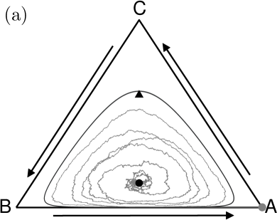
The nontrivial constant of motion governs the deterministic CLV dynamics characterized by regular oscillations associated with nested closed orbits surrounding in the phase space simplex Hofbauer and trajectories flowing according RMF06 , see Figs. 1 and 2.
The characteristics of the coexistence fixed point (center) and the neutrally stable orbits surrounding it’ mean that demographic fluctuations unavoidably perturb the dynamics predicted by (II.1) when . In fact, it has been shown that in a finite population, the CLV dynamics is characterized by stochastic trajectories that follow the deterministic orbits of (II.1) for a short transient whilst performing a random walk between them until the boundary of the phase space is reached, see Fig. 2. The internal noise thus leads to the extinction of two species after a characteristic time that depends on , while the individuals of the third species survive RMF06 . Hence, the survival probability of species is the probability that it reaches its absorbing state, with individuals of the species taking over, or fixating Kimura ; Ewens , the entire population 333In this context, the survival probability of a species coincides with its fixation probability. There has been a great interest in analyzing the influence of the population size on the species survival probabilities and mean extinction time (MET). In particular, the time-dependent extinction probability of two species was studied in Refs. RMF06 ; Dob12 , where the MET was shown to scale with the population size:
| (9) |
The survival probability, or fixation probability Kimura ; Ewens , when is not too small is independent of the initial condition Berr09 footnote1 and, with the population initially at (7), is defined by
| (10) |
When the reaction rates are equal, , all species have the same survival probability , independently of . Quite interestingly however, when the reaction rates are not all equal, the survival probability depends non-trivially on the population size Frean01 ; Berr09 . In fact, in sufficiently large but finite populations, the authors of Ref. Berr09 showed that the survival probabilities in the CLV model generally follow the so-called “law of the weakest” (LOW).
II.1.1 Survival probabilities in large populations and in the absence of external noise: the law of the weakest
The LOW says that the species that has the highest probability of being the surviving one in a sufficiently large population is the one with the lowest reproduction-predation rate, the “weakest species”:
| (11) |
The LOW becomes a “zero-one” law in the limit of very large populations (typically for ). It thus predicts that the weakest species has a probability one to survive at the expense of the others that go extinct (survival probability ). Hence, when is very large but finite the survival probability of species in the CLV is Berr09
| (12) | |||||
In Ref. Berr09 , the LOW was derived by studying the effect of demographic fluctuations on the outermost deterministic orbits set by (8). If two species have the same reaction rates that is less than the other, say , the zero-one version of the LOW predicts that and (i.e. and have probability to survive and almost certainly goes extinct).
II.1.2 Survival probabilities in small populations in the absence of external noise: the law of stay out
In addition to the LOW (11,II.1.1), a very different scenario emerges in small populations where the so-called law of stay out (LOSO) arises. This says that the most likely species to survive is the one predating on the species with the highest reproduction-predation rate (the strongest species) Berr09 :
| (13) | |||||
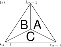
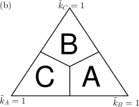
Contrary to Eq. (II.1.1), the LOSO is a non-strict law: for a given set of ’s, it says which species is the most likely to be the surviving one, but it does not assign a survival probability one to any of the species. When the population size is , the LOSO explicitly yields and Berr09 . Here, we have introduced the rescaled reaction rates in terms of which we can conveniently visualize the LOW and LOSO in , see Fig. 1.
II.1.3 Survival probabilities in the classical CLV: the law of the weakest and the law of stay out
In Ref. Berr09 a detailed analysis of the species survival probabilities has been carried out and it has been found that the survival probabilities follow the LOSO when , while they are predominantly determined by the LOW when (with asymptotic zero-one behavior typically when ). Intermediate scenarios interpolating between the LOSO and LOW have been reported when . For the model considered here in a static environment in which is the strongest species, the LOW predicts when while, according to the LOSO, species is the most likely to survive () in small populations.
The survival behavior of the CLV is known to be peculiar: In the LOW the weakest species prevails by favoring the spread of the predator of its own predator. The LOW and LOSO are thus specific to the cyclic competition of three species and no longer hold when the number of species exceeds three, see e.g. Refs. Durney11 ; Knebel13 . On the other hand, versions of the LOW have been found in other three-species systems, such as in the two-dimensional CLV (II) with mutation Tainaka93 . Below, we study the influence of environmental randomness on the survival behavior of the CLV.
III CLVDN & piecewise deterministic Markov process
In the presence of dichotomous noise, , the rate randomly switches according to (3) with (2) and . The CLVDN dynamics is thus governed by the ME (4), which is difficult to solve.
However, when , demographic fluctuations are negligible and the dynamics obeys the set of differential equations , , and , where depends on the DN, of amplitude (2). These coupled differential equations define a multivariate piecewise deterministic Markov process (PDMP), see, e.g., Refs. PDMP1 ; PDMP2 ; Ashcroft14 ; Hufton16 ; Hidalgo17 ; KEM17 . Hence, when the environmental state is , the reaction rates of species are , and for the average time that separates two environmental switches (), the CLVDN evolves according to the corresponding ODEs
| , | |||||
| (14) |
with when and when . Each environmental state is thus characterized by its own coexistence fixed point
| (15) |
with , and , and by its own conserved quantity
| (16) |
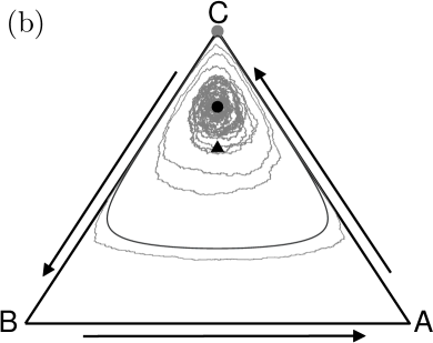
which define the two sets of closed orbits surrounding in each environmental state, see Fig. 2.
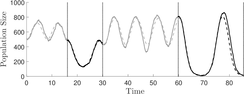
Hence, when the environment switches from to , the coexistence fixed point around which the orbits form and the CLVDN dynamics takes place moves from to , towards higher density of and lower densities of and , as shown in Figs. 2 and 3. When a switch occurs the dynamical flow settles on a new set of orbits that can be closer to the boundaries of the phase space, the amplitude and period of the oscillations change and the densities can suddenly be close to values or , as shown in Fig. 2 where we can see that .
The PDMP description (III) of the CLVDN dynamics is legitimate in an infinitely large population and provides a reasonably good approximation of the transient behavior in large but finite populations (see Fig. 3). As in the classical CLV (), whenever demographic fluctuations cause deviations from the PDMP trajectories and the CLVDN flows in thus consist of random walks between the two sets of orbits until an absorbing state is reached corresponding to the extinction of two species and the takeover by the surviving species.
IV Survival behavior in the CLVDN
Determining the survival probability of each species in the presence of random switching is an intriguing puzzle. In particular, it is not clear if/how the external noise affects the law of the weakest. We are thus particularly interested in the following question: Given , do the ’s satisfy the LOW relations (11) or (II.1.1) in a large population when ? If that is the case, we say that the LOW is followed also under external noise. Otherwise, we say that the LOW is not valid under external noise. Below, we shall see that different scenarios emerge below and above the environmental noise critical intensity defined as
| (17) |
where . Since here the LOW predicts when , the LOW is no longer valid as soon as the survival probability of species does not vanish in a large population.
To gain an understanding of the survival behavior of the CLVDN, in Figs. 4-6 we report extensive computer simulation results for the system (II)-(3) with and . In the examples of this section, the critical intensity is therefore , with when and when , while for all values of . Hence, when species and are the weakest in both environments, but when species and are the weakest in one environment and is in the other.
Our simulations have been carried out using the Gillespie algorithm Gillespie , which mirrors exactly the CLVDN dynamics prescribed by the ME (4). The survival probabilities and METs were calculated over runs for each value of , , and . Without loss of generality footnote1 , we started our simulations at the CLV coexistence fixed point (see Eq. (7)). We have considered sufficiently large systems () to be in the regime where the LOW holds in the absence of environmental noise, with , and predicts .
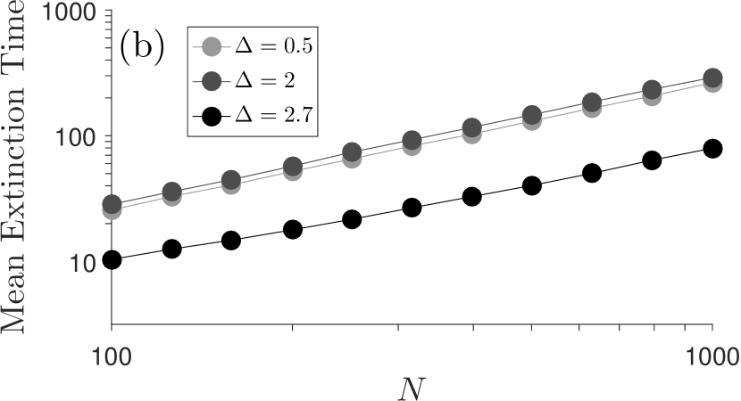
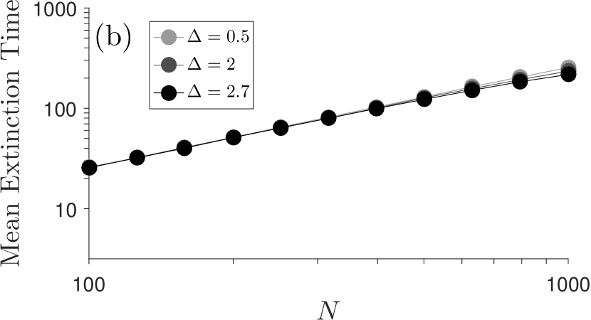
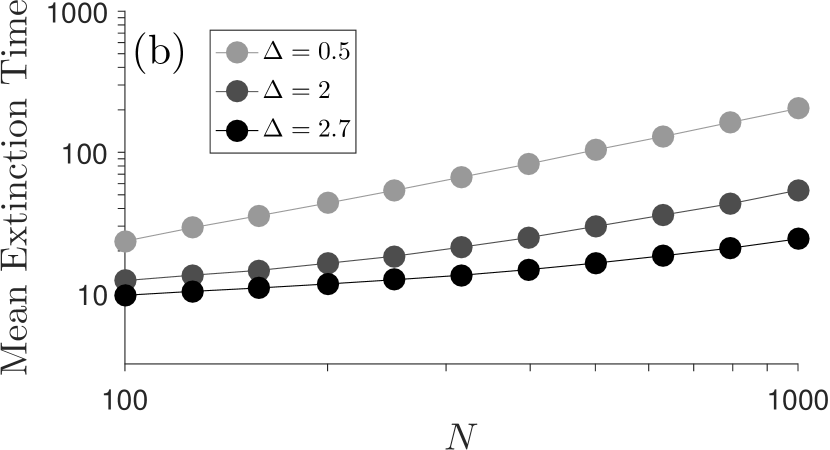
Simulation results of Figs. 4(a,b), 5(a,b), 6(a,b) confirm that the MET in the CLVDN scales with the population size in all regimes. (We verified that the MET conditioned on the extinction on a given species also scales with ). This can be explained as in the CLV RMF06 ; Berr09 ; Dob12 : extinction in the CLVDN results from a random walk between the nested orbits in the phase space driven by demographic noise (see Fig. 2). Yet in the CLVDN there are two types of orbits around : the erratic trajectories depend on the environment and change with and . However, it still generally takes a number of infinitesimal steps of order occurring at time increment to reach the edge of starting from the interior of the phase space. As a consequence, as in the classical CLV RMF06 ; Berr09 ; He10 ; Dob12 , the MET scales with , i.e. , as we have verified for in Figs 4(b), 5(b), 6(b). In practice, we have defined the MET to be the time that it takes for the one species to go extinct when the trajectory reaches the corresponding absorbing boundary.
Since the MET scales with the population size, and as the average time between two random switches is , the average number of switches of the reproduction-predation rate prior to extinction is of order . This suggests that our analysis should be carried out by discussing three different regimes: (a) the slow switching regime where (DN with long correlation time); (b) the fast switching regime where (DN with short correlation time); (c) and the intermediate switching regime where and the external noise has a finite correlation time (greater than zero).
IV.1 Slow-switching regime
In this regime, , and the external noise has a long correlation time . Hence, only very few or no switches occur prior to extinction. This means that in this regime the population is as likely to be locked into either of the environmental states (since ) until one species takes over and the others go extinct after a time of order . This can be used to determine the survival probabilities:
-
(i)
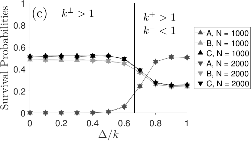
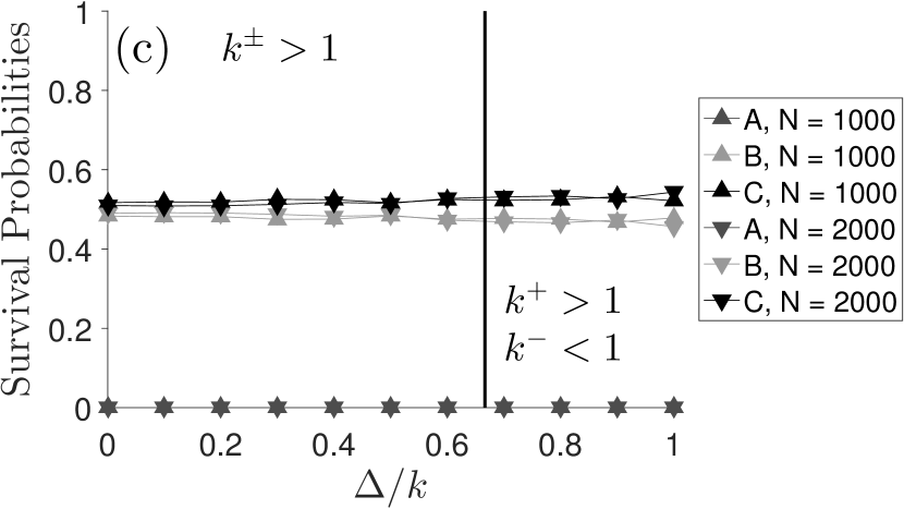
When and is sufficiently large, the LOW is followed because : and are the “weakest” species and therefore the most likely to survive in a large population, i.e. Berr09 . When , the LOW takes its zero-one form (II.1.1) and thus or is certain to be the sole species to survive whereas goes extinct: , as shown in Fig. 4(c).
-
(ii)
When , the LOW is not valid because and : When , and is the weakest species, whereas when , and is the strongest species. Since the population is as likely to be locked in either state , in half of the realizations species is the most likely to survive and in the others it is the least likely to survive. When , in the former case species is certain to be the sole surviving species, whereas in the latter situation it is guaranteed to go extinct while species and have the same probability to survive. Hence, when we find , which is in good agreement with the results of Fig. 4(c). So even though the LOW is valid in either environmental state, the fact that a realization is effectively locked in the state it starts in leads the LOW to not being valid overall.
-
(iii)
When , we have and . Hence, all species are as likely to survive when , while is the strongest species and therefore the least likely to survive when . When , this means that species is certain to go extinct in the environmental state . Taking into account that the system is equally likely to stay in either state , we find , as confirmed by Fig. 4(c).
Furthermore, in Fig. 4(c) the results for different values of are identical when is kept constant. One can proceed similarly if the rates are all different, say and finds that when , and when . These results indicate a transition occurring at , and that external noise alters the survival probabilities when : if the external noise is sufficiently strong, , no species is guaranteed to survive and the LOW is no longer valid.
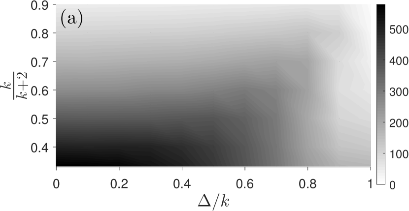
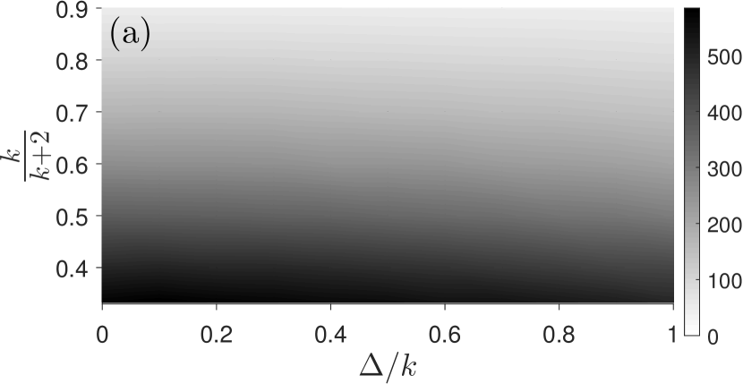
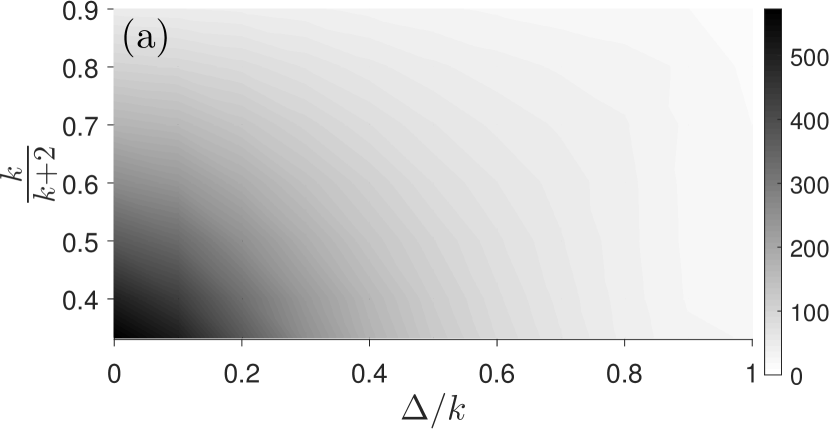
The results of the survival probabilities can qualitatively explain the MET dependence on and by noting that when and increase, moves toward the absorbing boundaries of species and while moves toward the absorbing boundary of species , see Fig. 2. When and , the system attains either the absorbing state of species or which takes longer from the orbits surrounding than from those around . Hence, when , the MET increases as increases (with fixed) because moves closer to the center of . However, when is kept fixed, decreases when increases and approaches the edges of . When and , there is a finite probability to reach any of the three absorbing states and this takes approximately the same time from any of the orbits surrounding which decreases as and increase (since approach the boundaries of ). Hence, the MET decreases when and increase and . The MET is maximal when , and it is minimal when .
IV.2 Fast-switching regime
In this regime, the environment varies rapidly with respect to the time scale of the population evolution. Hence, switches many times ( times, on average) before extinction occurs, and thus self-averages: HL06 ; Bena06 ; KEM17 . In this regime, the CLVDN is approximately identical to the CLV with reaction rates and therefore we note the following.
- (a)
-
(b)
Figs. 5(a,b) show that, in this regime, the MET is independent of due to the self-averaging, but it decays when increases and moves closer to the and absorbing boundaries, see Fig. 2(c). The MET is maximal when , and all species coexist with densities oscillating about the same values in the transient prior to extinction.
Again, we notice that in Fig. 5(c) the results for different values of are identical when is kept constant. In Fig. 5(c) we notice that is slightly greater than for all values of . This small effect stems from the influence of the LOSO (II.1.2) which says that in small population (without external noise), the species is more likely to survive than species and since here () and self averages. One can proceed similarly if the rates are all different, say , in which case, according to the zero-one LOW (II.1.1), we have .
IV.3 Intermediate-switching regime
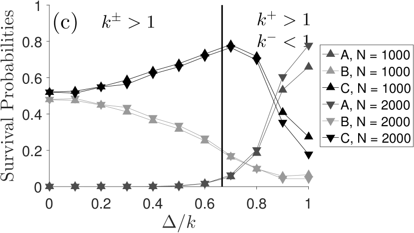
In this regime, the population composition and the environment vary on comparable time scales. On average, there are therefore a finite number of switches occurring prior to extinction and the environmental noise does not self-average. We therefore expect a markedly different survival behavior in this regime, where the external noise has a finite positive correlation time, than in the other regimes. For large but finite , in Fig. 6(c), we find the following:
-
(i)
When , is the strongest species and thus the least likely to survive according to the LOW, with , whereas when . However, increases and decreases when is raised from to .
-
(ii)
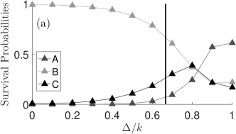
When , both and decrease when is raised, while increases with . Hence, when , species is the most likely to be the surviving one whereas species is the most likely to go extinct: . Therefore, under strong external noise, the species that is the strongest without environmental randomness (species ) is the most likely to prevail. In this case, the LOW is not valid since these results are in stark contrast with the predictions of the LOW for the CLV with reaction rates and .
-
(iii)
Surprisingly, the survival probability exhibits an intriguing non-monotonic dependence on and species is most likely to be the surviving one when , which we explain below. The results for different values of are identical when is kept constant.
-
(iv)
The MET decreases when increases because moves towards the absorbing boundaries of and . Additionally decreases as increases, as a result of the environmental switching changing the parts of the phase space that are more prone to extinction, as explained below.
To explain the intriguing behavior of reported in Fig. 6(c), we can adapt the arguments used in Ref. Berr09 to discuss the survival probabilities in the CLV. For this, the authors of Ref. Berr09 used the so-called outermost orbit obtained from (8) as the deterministic orbit that lies at a distance , i.e. one reproduction-predation reaction away, from the closest edge of . In the CLV, extinction arises once on the outermost orbit when a chance fluctuation pushes the trajectory along the edge of that drives it toward the absorbing state of the weakest species, yielding the LOW (Eq. II.1.1). Within a piecewise deterministic Markov process picture, we can adapt this argument to the CLVDN dynamics by considering two types of outermost orbits obtained from (see Eq. (16)): the orbit that surrounds (formed by the points satisfying ) and is associated with the environmental state , and that is at a distance from the and edges of when , or the edge of when , as shown in Figs. 2(a) (see also Fig. 7). The other outermost orbit (formed by the points satisfying ) surrounds and is associated with the environmental state , as shown in Fig. 2(b); it is at a distance from the and edges of . When , these two types of outermost orbits overlap greatly, see Fig. 7(a,b) where they are approximately equal except when the density of is small, whereas there is only a partial overlap when as shown in Fig. 7(c). These considerations help shed light on the -dependence of the fixation probabilities.
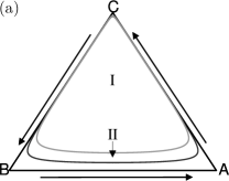
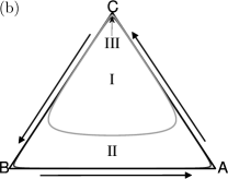
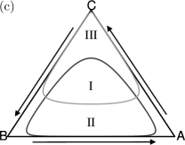
In fact, when , a typical CLVDN trajectory in performs a random walk around by approximately moving along the nested deterministic orbits and moving from one to another, see Figs. 2 and 3. When the environment switches, the orbit on which the trajectory is instantly changes, as does the coexistence fixed point. This results in a trajectory on an orbit that is either closer or further to the absorbing boundary of . As in the CLV Berr09 , if after a switch the trajectory lands outside the outermost orbit of the actual environmental state, internal fluctuations are likely to drive it to extinction into the closest absorbing state (if no other switches occur prior to extinction). This picture can be rationalized by considering the Regions I-III shown in Fig 7: Region II denotes the area within the outermost orbit that lies outside the outermost orbit. Region III is defined similarly for the part of within the outermost orbit, while Region I is the area contained within both outermost orbits. The dynamics in each of these regions is the following:
-
(a)
When there is a switch , the trajectories lying within Region II are outside the system’s outermost orbit and are very likely to flow along the edge and reach the absorbing state ().
-
(b)
Similarly, when a switch from occurs, the trajectories within Region III are outside the actual outermost orbit and therefore flow along the and edges to attain the absorbing state ().
-
(c)
All trajectories within Region I remain within the outermost orbit independently of the environmental state and their dynamics is essentially the same as in the CLV and dominated by internal noise. The LOW applies within Region I and in the case of Fig. 6(c) lead to the or absorbing state with probability ().
As a consequence, the area in Region I indicates the influence of the external noise in departing from the CLV-LOW scenario, while the areas of Regions II and III are associated with the probability of and being the sole surviving species. When is small (weak external noise), Regions I and II cover respectively a large and small part of while Region III is negligible, corresponding to , see Fig 7(a). Since Region II/I slightly increases/decreases when increases, increases with up to , see Fig 7(b). When , are well separated and all Regions I-III have a finite area corresponding to finite probabilities . When is increased further, the area of Region III grows and that within Region I and II shrink, see Fig 7(c). Hence, increases while and decrease with when , and species is the most likely to be the surviving one when the amplitude of the external noise is strong enough (for in Fig. 6(c)). This analysis explains the features of displayed in Fig. 6(c) and in particular, the non-monotonic -dependence of .
This can also explain the monotonic decrease of the MET for fixed : as increases, the fraction of the phase space contained in Regions II and III increases, so a larger amount of the phase space is more prone to extinction, reducing the expected time to extinction.
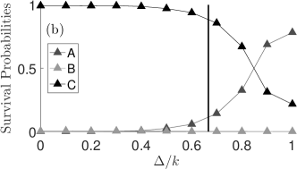
When , the results are similar: Fig. 8 shows the results for (a) and (b) . In the first case is the most likely species to survive without external noise (EN), and as the intensity of the EN is increased decreases, while increases after and increases then decreases. The only difference with Fig. 6(c) is that reaches its peak slightly after . When , species is the surviving one with probability in the absence of EN, so when and then is reduced as the EN intensity increases, with most of the variation occurring after , when increases ( for all values of ). Thus the non-monotonic dependence of on is a robust non-trivial joint effect of internal and environmental noise.
IV.4 CLVDN survival probabilities in small populations
In the CLV, the survival probabilities obey the law of stay out (LOSO), see Eqs. (II.1.2) and Fig. 1, in small systems, typically for Berr09 . It has also been found that the LOSO quantitatively influences in populations of greater size Berr09 . Here, we study the CLVDN survival probabilities in small populations in order to understand how external noise alters the LOSO. In particular, given , we ask whether the ’s satisfy the LOSO relations (II.1.2) in a small population when . When it is the case, we say that the LOSO is followed, otherwise the LOSO is not valid when .
To address this question, we first consider a population of size . Proceeding as described in Appendix B, we find
| (18) | |||||
| (19) |
where . Clearly, in the absence of external noise () one recovers the LOSO (II.1.2) according to which when, as in this section, . However, it is clear from (19) that when , it is only when , that . Hence, even when , the LOSO is followed only at sufficiently low and/or at high enough , but is generally not valid. The results (18),(19) indicate that determining which of or is the species to be the most likely to survive in small systems of size depends non trivially on and on ’s. Hence, the LOSO is generally not valid for small systems in the presence of environmental noise, and there is no simple general “law” to predict which species is most likely to survive in small populations when . An exception arises in the fast-switching regime, , when the noise self-averages and one recovers the LOSO (II.1.2) for . It has also to be noticed that for such small systems, the initial condition becomes relevant. What is more important for our purpose here, is that we have confirmed that, as for the CLV, coherent large-system scenarios emerge also in the CLVDN when . Hence, small-size effects are marginal in systems of size that we have considered in sections IV.1, IV.2 and IV.3.
V CLVDN survival behavior: Summary of the dependence on and
We now summarize the CLVDN survival behavior as a function of the population size , which controls the demographic noise, and of the external noise parameters and . We have always found that the (unconditional) mean extinction time scales linearly with the population size, i.e. , independently of the initial condition (when it is well separated from the absorbing boundaries), see Figs. 4(a,b), 5(a,b), 6(a,b). While we always find , as explained in Sec. IV, the MET is shortened when the intensity of the external noise increases.
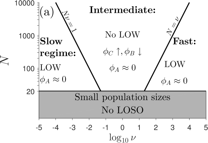
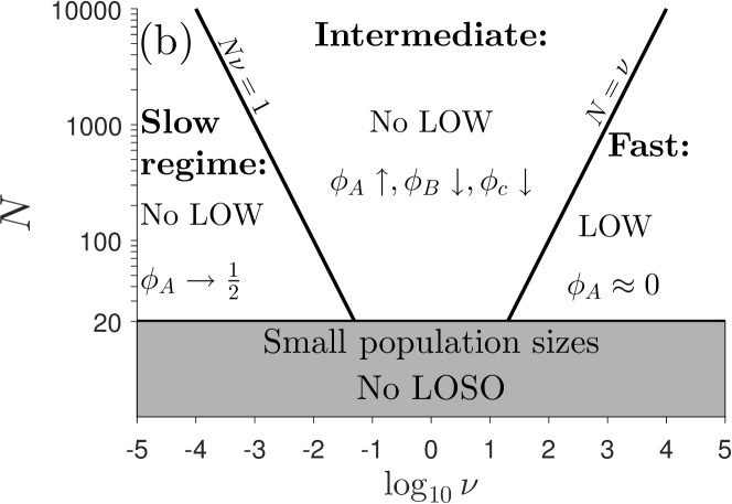
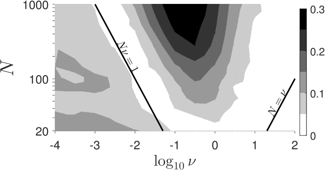
The species survival probabilities depend greatly on and on the average number of switches, of order , occurring prior to extinction. Except under fast switching, when the external noise self-averages and the law of the weakest holds, non-LOW scenarios emerge both below and above the critical EN intensity . In fact, when and , we find
-
•
When : Species is almost certain to go extinct for all values of . The LOW holds only in slow switching regime where . In the intermediate-switching regime, , decreases and grows when increases and no species is guaranteed to survive according to a non-LOW scenario, see Fig. 9(a).
-
•
When : Under slow switching, no species is guaranteed to survive and when the intensity of the EN is high (). Under intermediate-switching, increases while and decrease when increases according to a non-LOW scenario. Hence, species is the most likely to be the surviving one under external noise of high intensity () and switching rate , see Figs. 6(b), 8 and Fig. 9(b).
-
•
When : the main influence of the external noise occurs in the intermediate-switching regime, as illustrated Fig. 9(c) where is much greater than in the CLV when . This figure also shows that in the slow switching regime (left-hand light gray area), and in the fast switching regime (right-hand white area).
While we have focused on , the above results also hold for when , in which case the scenarios summarized in Fig. 9(b) for arise. In populations of small size, , the survival probabilities depend in an intricate way of and generally do not follow neither the LOSO nor the LOW.
VI Conclusion
We have investigated the joint effect of environmental randomness and demographic fluctuations on the survival (or, equivalently, fixation) behavior of the paradigmatic cyclic Lotka-Volterra model in which each of three species, and , is in turn the predator and the prey of another species. When the population is large but finite, and the environment is static (no external noise), the survival probabilities have been shown to obey the so-called “law of the weakest” Berr09 ; Frean01 ; Ifti03 ; RMF06 : the “weakest species” (with the lowest reproduction-predation rate) is the most likely to be the surviving one, with a survival probability that asymptotically approaches one. The other species go extinct in a time scaling with the population size.
While the law of the weakest generally does not hold when more than three species interact, variants of this law have been found in a number of three-species systems exhibiting cyclic competition. Here, we have assessed the robustness of the law of the weakest against a simple form of environmental randomness in the cyclic Lotka Volterra model. For this, we have modeled environmental variability by considering the random switching of the reproduction-predation of the strongest species in a static environment, , between two values corresponding to more and less favorable environmental conditions. We have analyzed how the joint effect of environmental and demographic noise affects the survival probabilities, and how the presence of external noise alters the law of the weakest that predicts the certain extinction of species in a static environment.
We have found that in a large population, under external noise of sufficient intensity and for a dichotomous noise whose switching rate is not too high, the law of the weakest is violated and no zero-one law holds, hence no species is guaranteed to survive. In fact, new survival scenarios emerge under sufficiently strong external noise and/or when the rate of switching is not too high. When the environment switches very slowly, the population is likely to stay in its initial (randomly distributed) environmental state and, above an external noise intensity threshold, species is either the weakest (where the LOW predicts that it survives with probability ) or the strongest (where the LOW predicts that it goes extinct). This results in its finite probability (about ) of being the surviving species, which is different to the LOW when the intensity of the external noise vanishes (), even though it is followed in each environment. A complex survival scenario emerges when the environment and the population evolve on similar time scales: the survival probability of the predator (species ) of species typically exhibits a non-monotonic dependence on the external noise intensity, while the survival probability of increases with the strength of the environmental noise, and is the most likely to survive under strong external noise. These surprising results have been explained by considering the possible paths to extinction from the “outermost orbits” characterizing the dynamics described by the underpinning piecewise deterministic Markov process. The survival probabilities follow the law of the weakest when the random switching occurs on a much faster time scale than the population relaxation, and when both the external noise intensity and the switching rate are low. In the former case, there are many switches prior to extinction and their effect averages out, while in the latter remains the strongest species in each environmental state and is thus almost certain to go extinct. We have also found that the mean extinction time always scales with the population size, and the general effect of the external noise is to reduce the subleading contribution to the mean extinction time.
Our findings demonstrate that even a simple form of external noise drastically alter the survival probabilities of a reference system like the cyclic Lotka-Volterra model and, together with demographic noise, leads to complex survival scenarios. Here, for the sake of simplicity, we have concentrated on the cyclic Lotka-Volterra dynamics characterized by neutrally stable deterministic orbits. However, we expect that a similar analysis would in principle also apply to the case where the coexistence of the species is deterministically stable or leads to heteroclinic cycles MayLeonard . In these cases also, the path to extinction occurs along cyclic trajectories close to the absorbing boundary. However, these paths are difficult to determine in the absence of a conserved quantity, and, when coexistence is deterministically stable, the mean extinction time typically increases exponentially with the system size.
VII Acknowledgments
The support of an EPSRC PhD studentship (Grant No. EP/N509681/1) is gratefully acknowledged.
Appendix A Survival probabilities in the CLVDN with three randomly switching reaction rates
For the sake of simplicity, we have focused on the case where only one reaction rate, , randomly switches. However, it is realistic to assume that the reaction rates of all species are subject to environmental variability. In general, each , with , would be affected by different external factors, leading to a CLVDN (II) with
| (20) |
where and are independent dichotomous noise variables, such that , each with a distinct switching rate and intensities , , . Each in (20) has the same properties as of Sec. II, e.g., . The CLVDN with (20) spans a large-dimensional parameter space that is difficult to scrutinize.
In this appendix, for the sake of concreteness, we show that the results obtained so far can be of direct relevance for the general model (II) with noisy rates (20) when these fluctuate on markedly different timescales. Here, we assume , with , and we set . This corresponds to the situation where species and are subject external factors changing with high and low frequency, respectively, while the growth rate of species changes with factors varying on the same times scale on which the population composition changes. Since switches fast () and switches slowly (), from Sec. IV, we expect to self-average and thus simply consider that , while (when ) or (when ), each with a probability .
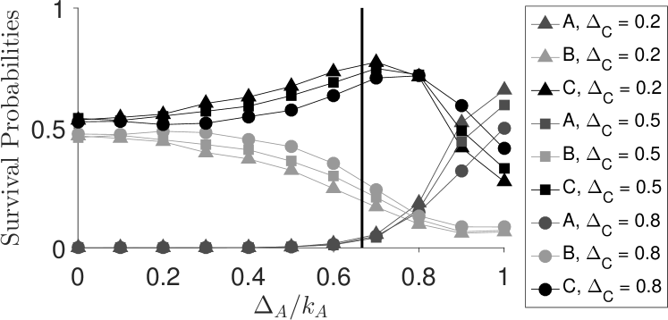
By denoting here and , we can thus make contact with the results of Sec. IV.3.
When , we have and the survival behavior is similar to that of Sec. IV.3 as shown by Fig. 10 whose similarities with Fig. 6(b) are striking: and respectively increases and decreases with while . Hence, as in Sec. IV.3, species is the most likely to be the surviving one under external noise of low intensity while is the “strongest” species and therefore the most likely to go extinct. When , and which also yields the same qualitative behavior as in Fig. 6(c): and increase and decreases with while varies non-monotonically with . For the same reason explained in Sec. IV.3, species becomes the most likely to survive under strong external noise. A noticeable, yet marginal, difference between Figs. 6(c) and 10 is the fact that the is maximum for in Fig. 10 instead of . In Fig. 10 the peak of moves towards higher values of because is the “weakest” species under strong EN in the environmental states when .
Appendix B Derivation of the CLVDN survival probabilities when
In this appendix, we consider the CLVDN in a system of size and determine the species survival probabilities. In this system, the fate of the system is completely determined by the first reaction that takes place, after which an absorbing boundary is reached and only one species survives. Starting with one individual of each species, if replaces then is the sole surviving species. Similarly, if replaces then will be the survive, and if replaces then will survive. Hence, when the species that survives is completely determined by the first reproduction-predation reaction that occurs. Here, we proceed with the derivation of ( and follow analogously): survives if the first reproduction-predation reaction is the reaction. Hence the probability that is the surviving species is
where stands for “probability of ”.
We consider first that initially and according to (B), with and , we have
The case of the initial state is treated similarly and yields . Since, the population is initially as likely to be in either of the environmental states, we have
Proceeding similarly for and , we obtain (19).
References
- (1) R. M. May, Stability and Complexity in Model Ecosystems (Princeton University Press, Princeton, New Jersey, 1974).
- (2) S. P. Hubbell, The Unified Neutral Theory of Biodiversity and Biogeography (Princeton University Press, Princeton, New Jersey, 2001).
- (3) E. Pennisi, Science, 309, 90 (2005).
- (4) N. G. Van Kampen, Stochastic Processes in Physics and Chemistry (Elsevier, Amsterdam, Netherlands, 1992).
- (5) C. Gardiner, Handbook of Stochastic Methods (Springer, New York, U.S.A., 2002).
- (6) J. F. Crow and M. Kimura, An Introduction to Population Genetics Theory (Blackburn Press, New Jersey, 2009).
- (7) W. J. Ewens, Mathematical Population Genetics (Springer, New York, 2004).
- (8) T. Reichenbach, M. Mobilia and E. Frey, Phys. Rev. E 74, 051907 (2006).
- (9) M. Berr, T. Reichenbach, M. Schottenloher and E. Frey, Phys. Rev. Lett. 102, 048102 (2009).
- (10) E. Frey, Physica A, 389, 4265 (2010).
- (11) T. Reichenbach, M. Mobilia and E. Frey, Nature (London) 448, 1046 (2007).
- (12) B. Kerr, M. A. Riley, M. W. Feldman, and B. J. M. Bohannan, Nature (London) 418, 171 (2002).
- (13) B. Sinervo and C. M. Lively, Nature (London) 380, 240 (1996).
- (14) J. B. C. Jackson and L. Buss, Proc. Nat. Acad. Sci. USA, 72, 5160 (1975).
- (15) R. M. May and W. J. Leonard, SIAM J. Appl. Math. 29, 243 (1975).
- (16) J. Maynard Smith, Evolution and the Theory of Games (Cambridge University Press, Cambridge , U.K.).
- (17) A. Szolnoki, M. Mobilia, L.-L. Jiang, B. Szczesny, A. M. Rucklidge, and M. Perc, J. R. Soc. Interface 11, 20140735 (2014).
- (18) U. Dobramysl, M. Mobilia, M. Pleimling, and U. C. Täuber, J. Phys. A: Math. Theor. 51, 063001 (2018)
- (19) T. Reichenbach, M. Mobilia, and E. Frey, Nature (London) 448, 1046 (2007).
- (20) T. Reichenbach, M. Mobilia, and E. Frey, Phys. Rev. Lett. 99, 238105 (2007).
- (21) T. Reichenbach, M. Mobilia, and E. Frey, J. Theor. Biol. 254, 368 (2008).
- (22) Q. He, M. Mobilia, and U. C. Täuber, Phys. Rev. E 82, 051909 (2010).
- (23) Q. He, M. Mobilia, and U. C. Täuber, Eur. Phys. J. B 82, 97 (2011).
- (24) M. Mobilia, J. Theor. Biol. 264, 1 (2010).
- (25) B. Kerr, C. Neuhauser, B. J. M. Bohannan, and A. M. Dean, Nature (London) 442, 75 (2006).
- (26) M. Peltomäki and M. Alava, Phys. Rev. E 78, 031906 (2008).
- (27) T. Reichenbach and E. Frey, Phys. Rev. Lett. 101, 058102 (2008).
- (28) B. Szczesny, M. Mobilia and A. M. Rucklidge, EPL (Europhysics Letters) 102, 28012 (2013).
- (29) B. Szczesny, M. Mobilia and A. M. Rucklidge, Phys. Rev. E 90, 032704 (2014).
- (30) B. Szczesny, PhD Dissertation, University of Leeds (2014).
- (31) M. Mobilia, A. M. Rucklidge, and B. Szczesny, Games 7, 24 (2016).
- (32) C. M. Postlethwaite and A. M. Rucklidge, EPL (Europhysics Letters) 117, 48006 (2017)
- (33) J. Hofbauer and K. Sigmund, K., Evolutionary games and population dynamics (Cambridge University Press, U.K., 1998).
- (34) R. M. Nowak, Evolutionary Dynamics (Belknap Press, Cambridge, USA, 2006).
- (35) M. Broom and J. Rychtář, Game-Theoretical Models in Biology (CRC Press, Boca Raton, USA, 2013).
- (36) M. Frean; E. D. Abraham, Proc. R. Soc. Lond. B 268, 1323 (2001).
- (37) M. Ifti and B. Bergensen, Eur. Phys. J. E, 10, 241 (2003).
- (38) T. Reichenbach, M. Mobilia, and E. Frey, Banach Centre Publications 80, 259 (2008).
- (39) K. I. Tainaka, Phys. Rev. Lett. 63, 2688 (1989).
- (40) K. I. Tainaka, Phys. Lett. A 176, 303 (1993).
- (41) K. I. Tainaka, Phys. Rev. E 50, 3401 (1994).
- (42) L. Frachebourg, P. L. Krapivsky, and E. Ben-Naim, Phys. Rev. Lett. 77, 2125 (1996).
- (43) G. Szabó and A. Szolnoki, Phys. Rev. E 65, 036115 (2002).
- (44) M. Perc, A. Szolnoki, and G. Szabó, Phys. Rev. E 75, 052102 (2007).
- (45) X. Ni, W. X. Wang, Y. C. Lai, and C. Grebogi, Phys. Rev. E 82, 066211 (2010).
- (46) S. Venkat and M. Pleimling, Phys. Rev. E 81, 021917 (2010).
- (47) A. Dobrinevski and E. Frey, Phys. Rev. E 85, 051903 (2012).
- (48) N. Mitarai, I. Gunnarson, B. N. Pedersen, C. A. Rosiek, and K. Sneppen, Phys. Rev. E 93, 042408 (2016).
- (49) R. Levins, Evolution in Changing environments: some Theoretical Explorations (Princeton University Press, Princeton, New Jersey, 1968).
- (50) W. M. Schaffer, Am. Nat. 108, 783 (1974).
- (51) C. R. Morley, J. A. Trofymow, D. C. Coleman, and C.Cambardella, Microbiol. Ecol. 9, 329 (1983).
- (52) C. A. Fux, J. W. Costerton, P. S. Stewart, and P. Stoodley, Trends Microbiol. 13, 34 (2005).
- (53) P. L. Chesson and R. R. Warner, Am. Nat. 117, 923 (1981).
- (54) N. Q. Balaban, J. Merrin, R. Chait, L. Kowalik, and S. Leibler, Science 305, 1622 (2004).
- (55) E. Kussell, R. Kishony, N. Q. Balaban, and S. Leibler, Genetics 169, 1807 (2005).
- (56) M. Acer, J. Mettetal, and A. van Oudenaarden, Nature Genetics 40, 471 (2008);
- (57) H. Beaumont, J. Gallie, C. Kost, G. Ferguson, and P. Rainey, Nature 462, 90 (2009).
- (58) U. Dobramysl, and U. C. Täuber, Phys. Rev. Lett. 110, 048105 (2013).
- (59) S. Karlin and B. Levikson, T. Pop. Biol. 6, 383 (1974).
- (60) M. Assaf, E. Roberts, Z. Luthey-Schulten, and N. Goldenfeld, Phys. Rev. Lett. 111, 058102 (2013).
- (61) M. Assaf, M. Mobilia, and E. Roberts, Phys. Rev. Lett. 111, 238101 (2013).
- (62) P. Ashcroft, P. M. Altrock, and T. Galla, J. R. Soc. Interface 11, 20140663 (2014).
- (63) A. Melbinger and M. Vergassola, Scientific Reports 5, 15211 (2015).
- (64) M. Danino, N. M. Shnerb, S. Azaele, W. E. Kunin, and D. A. Kessler, J. Theor. Biol. 409, 155 (2016).
- (65) M. Thattai and A. Van Oudenaarden, Proc. Natl. Acad. Sci. USA 98, 8614 (2001).
- (66) E. Kussell and S. Leibler, Science 309, 2075 (2005).
- (67) P. G. Hufton, Y. T. Lin, T. Galla, and A. J. McKane, Phys. Rev. E 93, 052119 (2016).
- (68) J. Hidalgo, S. Suweis, and A. Maritan, J. Theor. Biol. 413, 1 (2017).
- (69) B. K. Xue and S. Leibler, Phys. Rev. Lett. 119, 108103 (2017).
- (70) K. Wienand, E. Frey, and M. Mobilia, Phys. Rev. Lett. 119, 158301 (2017).
- (71) K. Wienand, E. Frey, and M. Mobilia, e-print: https://arxiv.org/abs/1712.07939.
- (72) K. Sato, N. Konno and T. Yamaguchi, Mem. Muroram Inst. Tech. 47, 109-114 (1997).
- (73) A. Szolnoki and G. Szabó, Phys. Rev. E, 70 037102 (2004).
- (74) G. Szabó, A. Szolnoki, and R. Izsák , J. Phys. A: Math. Gen. 37 2599 (2004).
- (75) C. Spalding, C. R. Doering, and G. R. Flierl, e-print: https://arxiv.org/abs/1710.06274.
- (76) M. Danino and N. M. Shnerb, e-print: https://arxiv.org/abs/1710.08807.
- (77) W. Horsthemke and R. Lefever, Noise-Induced Transitions (Springer, Berlin, 2006).
- (78) I. Bena, Int. J. Mod. Phys. B 20, 2825 (2006).
- (79) C. H. Durney, S. O. Case, M. Pleimling, and R. K. P. Zia, Phys. Rev. E 83, 051108 (2011).
- (80) J. Knebel, T. Krüger, M. F. Weber, and E. Frey Phys. Rev. Lett. 110 168106 (2013).
- (81) K. Kitahara, W. Horsthemke, and R. Lefever, Phys. Lett. 70A, 377 (1979).
- (82) M. H. A. Davis, J. R. Stat. Soc. B 46, 353 (1984).
- (83) D. T. Gillespie, J. Comput. Phys. 22, 403 (1976).
- (84) If initially, the number of individuals of species is , the survival probability is . However, except for special initial states (e.g, close to the boundaries), is independent of the initial condition, and the same holds for the mean extinction time . Here, as in Ref. RMF06 ; Berr09 , we obtain results that are independent of the initial condition and thus define by (10).