Central limit theorems for entropy-regularized optimal transport on finite spaces and statistical applications 111This work has been carried out with financial support from the French State, managed by the French National Research Agency (ANR) in the frame of the GOTMI project (ANR-16-CE33-0010-01).
Abstract
The notion of entropy-regularized optimal transport, also known as Sinkhorn divergence, has recently gained popularity in machine learning and statistics, as it makes feasible the use of smoothed optimal transportation distances for data analysis. The Sinkhorn divergence allows the fast computation of an entropically regularized Wasserstein distance between two probability distributions supported on a finite metric space of (possibly) high-dimension. For data sampled from one or two unknown probability distributions, we derive the distributional limits of the empirical Sinkhorn divergence and its centered version (Sinkhorn loss). We also propose a bootstrap procedure which allows to obtain new test statistics for measuring the discrepancies between multivariate probability distributions. Our work is inspired by the results of Sommerfeld and Munk in [32] on the asymptotic distribution of empirical Wasserstein distance on finite space using unregularized transportation costs. Incidentally we also analyze the asymptotic distribution of entropy-regularized Wasserstein distances when the regularization parameter tends to zero. Simulated and real datasets are used to illustrate our approach.
1 Introduction
1.1 Motivations
In this paper, we study the convergence (to their population counterparts) of empirical probability measures supported on a finite metric space with respect to entropy-regularized transportation costs. Transport distances are widely employed for comparing probability measures since they capture in a instinctive manner the geometry of distributions (see e.g [36] for a general presentation on the subject). In particular, the Wasserstein distance is well adapted to deal with discrete probability measures (supported on a finite set), as its computation reduces to solve a linear program. Moreover, since data in the form of histograms may be represented as discrete measures, the Wasserstein distance has been shown to be a relevant statistical measure in various fields such as clustering of discrete distributions [39], nonparametric Bayesian modelling [23], fingerprints comparison [32], unsupervised learning [1] and principal component analysis [3, 30, 5].
However, the computational cost to evaluate a transport distance is generally of order for discrete probability distributions with a support of size . To overcome the computational cost to evaluate a transport distance, Cuturi [7] has proposed to add an entropic regularization term to the linear program corresponding to a standard optimal transport problem, leading to the notion of Sinkhorn divergence between probability distributions. Initially, the purpose of transport plan regularization was to efficiently compute a divergence term close to the Wasserstein distance between two probability measures, through an iterative scaling algorithm where each iteration costs . This proposal has recently gained popularity in machine learning and statistics, as it makes feasible the use of smoothed optimal transportation distance for data analysis. It has found various applications such as generative models [19] and more generally for high dimensional data analysis in multi-label learning [16], dictionary learning [28], image processing [9, 25], text mining via bag-of-words comparison [18], averaging of neuroimaging data [20].
The goal of this paper is to analyze the potential benefits of the Sinkhorn divergence and its centered version [14, 19] for statistical inference from empirical probability measures. We derive novel results on the asymptotic distribution of such divergences for data sampled from (unknown) distributions supported on a finite metric space. The main application is to obtain new test statistics (for one or two samples problems) for the comparison of multivariate probability distributions.
1.2 Previous work and main contributions
The derivation of distributional limits of an empirical measure towards its population counterpart in -Wasserstein distance is well understood for probability measures and supported on [15, 10, 11]. These results have then been extended for specific parametric distributions supported on belonging to an elliptic class, see [27] and references therein. Recently, a central limit theorem has been established in [12] for empirical transportation cost, and data sampled from absolutely continuous measures on , for any . The case of discrete measures supported on a finite metric space has also been considered in [32] with the proof of the convergence (in the spirit of the central limit theorem) of empirical Wasserstein distances toward the optimal value of a linear program. Additionally, Klatt et al. [21] analyzed, in parallel with our results, the distributional limit of regularized optimal transport divergences between empirical distributions. In particular, the work in [21] extends the study of distributional limits of regularized empirical transportation cost to general penalty functions (beyond entropy regularization). The authors of [26] also studied the link between nonparametric tests and the Wasserstein distance, with an emphasis on distributions with support in .
However, apart from the one-dimensional case (), and the work of [21], these results lead to test statistics whose numerical implementation become prohibitive for empirical measures supported on with . The computational cost required to evaluate a transport distance is indeed only easily tractable in . It is therefore of interest to propose test statistics based on fast Sinkhorn divergences [7]. In this context, this paper focuses on the study of inference from discrete distributions in terms of entropically regularized transport costs, the link with the inference through unregularized transport, and the construction of tests statistics that are well suited to investigate the equality of two distributions. The results are inspired by the work in [32] on the asymptotic distribution of empirical Wasserstein distance on finite space using unregularized transportation costs.
Our main contributions may be summarized as follows. First, for data sampled from one or two unknown measures and supported on a finite space, we derive central limit theorems for the Sinkhorn divergence between their empirical counterpart. These results allow to build new test statistics for measuring the discrepancies between multivariate probability distributions. Notice however that the Sinkhorn divergence denoted (where is a regularization parameter) is not a distance since . This is a serious drawback for testing the hypothesis of equality between distributions. Thus, as introduced in [14, 19], we further consider the centered version of the Sinkhorn divergence , referred to as Sinkhorn loss, which satisfies . This study thus constitutes an important novel contribution with respect to the work of [21]. We present new results on the asymptotic distributions of the Sinkhorn loss between empirical measures. Interestingly, under the hypothesis that , such statistics do not converge to a Gaussian random variable but to a mixture of chi-squared distributed random variables. To illustrate the applicability of the method to the analysis of real data, we propose a bootstrap procedure to estimate unknown quantities of interest on the distribution of these statistics such as their non-asymptotic variance and quantiles. Simulated and real datasets are used to illustrate our approach. Finally, one may stress that an advantage of the use of test statistics based regularized Wasserstein distance (rather than other losses or divergences) is to allow further statistical inference from the resulting optimal transport plan as demonstrated in [21] for the analysis of protein interaction networks.
1.3 Overview of the paper
In Section 2, we briefly recall the optimal transport problem between probability measures, and we introduce the notions of Sinkhorn divergence and Sinkhorn loss. Then, we derive the asymptotic distributions for the empirical Sinkhorn divergence and the empirical Sinkhorn loss. We also give the behavior of such statistics when the regularization parameter tends to zero at a rate depending on the number of available observations. A bootstrap procedure is discussed in Section 3. Numerical experiments are reported in Section 4 for synthetic data and in Section 5 for real data.
2 Distributional limits for entropy-regularized optimal transport
In this section, we give results on the asymptotic distributions of the empirical Sinkhorn divergence and the empirical Sinkhorn loss. The proofs rely on the use of the delta-method and on the property that is a differentiable function with respect to and .
2.1 Notation and definitions
We first introduce various notation and definitions that will be used throughout the paper.
2.1.1 Optimal transport, Sinkhorn divergence and Sinkhorn loss
Let be a complete metric space with . We denote by the set of Borel probability measures supported on with finite moment of order , in the sense that is finite for some (and thus for all) . The -Wasserstein distance between two measures and in is defined by
| (1) |
where the infimum is taken over the set of probability measures on the product space with respective marginals and .
In this work, we consider the specific case where is a finite metric space of size . In this setting, a measure is discrete, and we write where is a vector of positive weights belonging to the simplex and is a Dirac measure at location . Therefore, computing the -Wasserstein distance between discrete probability measures supported on amounts to solve a linear program whose solution is constraint to belong to the convex set . However, the cost of this convex minimization becomes prohibitive for moderate to large values of . Regularizing a complex problem with an entropy term is a classical approach in optimization to reduce its complexity [38]. This is the approach followed in [7] by adding an entropy regularization to the transport matrix, which yields the strictly convex (primal) problem (2) presented below.
As the space is fixed, a probability measure supported on is entirely characterized by a vector of weights in the simplex. By a slight abuse of notation, we thus identify a measure by its vector of weights (and we sometimes write ).
Definition 2.1 (Sinkhorn divergence).
Let be a regularization parameter. The Sinkhorn divergence [7] between two probability measures and in is defined by
| (2) |
where denotes the usual inner product between matrices, denotes the tensor product and
- -
-
is the set of transport matrices with marginals and (with denoting the vector of with all entries equal to one) ,
- -
-
is the pairwise cost matrix associated to the metric space whose -th entry is ,
- -
-
the regularization function is the relative entropy for a transport matrix .
Remark 1.
This entire section is also valid for symmetric positive cost matrices for which .
The dual version of problem (2) is introduced in the following definition.
Definition 2.2 (Dual problem).
It is now well known that there exists an explicit relationship between the optimal solutions of primal (2) and dual (3) problems. These solutions can be computed through an iterative method called Sinkhorn’s algorithm [8] that is described below and which explicitly gives this relationship.
Proposition 2.1 (Sinkhorn’s algorithm).
Let be the elementwise exponential of the matrix cost divided by minus the matrix with all entries equal to . Then, there exists a pair of vectors such that the optimal solutions and of problems (2) and (3) are respectively given by
where is the pointwise multiplication. Moreover, such a pair is unique up to scalar multiplication (or equivalently is unique up to translation), and it can be recovered as a fixed point of the Sinkhorn map
| (4) |
where is the transpose of and stands for the component-wise division.
Remark 2.
When the cost matrix is defined as and the grid points are uniformly spread, the matrix vector products involving within the Sinkhorn algorithm can be efficiently performed via separated one dimensional convolutions [31] without storing .
As discussed in the introduction, an important issue regarding the use of Sinkhorn divergence for testing the equality of two distributions is that it leads to a biased statistics in the sense that is not equal to zero under the null hypothesis . A possible alternative to avoid this issue is to consider the so-called notion of Sinkhorn loss [14, 19] as defined below.
Definition 2.3 (Sinkhorn loss).
Let be a regularization parameter. The Sinkhorn loss between two probability measures and in is defined by
| (5) |
The Sinkhorn loss is not a distance between probability distributions, but it satisfies various interesting properties for the purpose of this paper, that are summarized below.
Proposition 2.2.
The Sinkhorn loss satisfies the following three key properties (see Theorem 1 in [14]):
-
(i)
,
-
(ii)
,
-
(iii)
.
From Proposition 2.2, we have that is equivalent to , therefore the function reaches its global minimum at , implying that the gradient of the Sinkhorn loss is zero when which is summarized in the following corollary.
Corollary 2.4.
For any , the gradient of the Sinkhorn loss satisfies .
2.1.2 Statistical notations
We denote by the convergence in distribution of a random variable and the convergence in probability. The notation means that is a random variable taking its values in with law (namely that for each ). Likewise stands for the equality in distribution of the random variables and .
Let and and be the empirical measures respectively generated by iid samples and , that is
| (6) |
We also define the multinomial covariance matrix
and the independent Gaussian random vectors and . As classically done in statistics, we say that
2.1.3 Notations for differentiation
For a sufficiently smooth function , we denote by and the gradient and the hessian of the function . In particular, the gradient of at the point in the direction is denoted by (this notation also holds for the hessian). Moreover, the first-order partial derivative with respect to the first variable (resp. ) is given by (resp. ). Equivalently, the second-order partial derivative is denoted , with .
2.2 Differentiability of
As stated at the beginning of the section, the differentiability of (in the usual Fréchet sense) is needed in order to apply the delta-method. This is proved in the following proposition.
Proposition 2.3.
Proof.
From Proposition 2 in [14], is Gâteaux differentiable and its derivative reads
for . In order to prove its differentiability (or Fréchet differentiability, since is a finite dimensional space) at the point , we only need to prove that the operator is continuous (see e.g. Prop. 3.2.3. in [40]) in . Suppose that tends to when tends to infinity. Therefore, this convergence also holds in the weak∗ topology for the probability measures and . We denote by the unique couple in such that for an arbitrary . Then, we can apply Cauchy-Schwarz inequality and then use Proposition 13 in [14] on the convergence of the pair of dual variables towards (such that ), to obtain that
which concludes the proof. ∎
2.3 Distributional limits for the empirical Sinkhorn divergence
2.3.1 Convergence in distribution
The following theorem is our main result on distributional limits of empirical Sinkhorn divergences.
Theorem 2.5.
Proof.
Following the proof of Theorem 1 in [32], we have that (see e.g. Theorem 14.6 in [37])
since is a sample of a multinomial probability measure with probability . For the two samples case, we use that
where and are the quantities defined in the statement of Theorem 2.5. From Proposition 2.3, we can directly apply the delta-method:
| (9) |
while, for and tending to infinity such that and , we obtain that
| (10) |
This completes the proof of Theorem 2.5. ∎
2.3.2 Convergence in probability
Distributional limits of empirical Sinkhorn divergences may also be characterized by a convergence in probability by the following result which directly follows from the delta-method (see e.g. Theorem 3.9.4 in [35]).
Theorem 2.6.
The following asymptotic results hold for empirical Sinkhorn divergences, for any .
-
1.
One sample. As , one has that
-
2.
Two samples - For and as , one has that
Proof.
As the map is defined, linear and continuous on , Theorem 3.9.4 in [35] allows us to conclude. ∎
2.4 Distributional limits for the empirical Sinkhorn loss
2.4.1 Convergence in distribution
The following theorems are our main results on distributional limits of the empirical Sinkhorn loss, for which we now distinguish the cases (alternative hypothesis) and (null hypothesis).
Theorem 2.7.
Let be two probability distributions in . Let us denote by their empirical counterparts and by the dual variables which are the optimal solutions of the dual problem . Then, the following asymptotic results hold.
-
1.
One sample. As , one has that
(11) -
2.
Two samples. For and as , one has that
Proof.
Under the null hypothesis , the derivation of the distributional limit of either or requires further attention. Indeed, thanks to Proposition 2.2, one has that the function reaches its global minimum at , and therefore the gradient of the Sinkhorn loss satisfies . Hence, to obtain the distributional limit of the empirical Sinkhorn loss it is necessary to apply a second-order delta-method yielding an asymptotic distribution which is not Gaussian anymore.
Theorem 2.8.
Let be a probability distribution on , and denote by an empirical measures obtained by independent sampling data from . Then, as tends to infinity, the following asymptotic result holds
| (13) |
where are the non-negative eigenvalues of the matrix
and are independent random variables with chi-squared distribution of degree .
Proof.
From Corollary 2.4, we have that . In order to apply a second order delta-method, the Hessian matrix of the Sinkhorn loss needs to be non-singular in the neighborhood of . Note that the Sinkhorn loss is at least (admitting a third continuous differential) on the interior of its domain, as proved in Theorem 2 by [22]. Moreover, since the function is -strongly convex (Theorem 3.4, [2]) and is (strictly) convex (Proposition 4, [14]), we have that the Hessian matrix of is non-singular. We can thus apply Theorem 17 in [33] which states that from second order delta-method, the distributional limits of is given by
that can be rewritten as
where are the eigenvalues of the matrix . This concludes the distributional limit presented in relation (13). ∎
In the two samples case, the Hessian matrix is not guaranteed to be non-singular, in which case the asymptotic distribution is degenerated. Nevertheless, we have the following theorem.
Theorem 2.9.
Let be a probability distribution on , and denote by two empirical measures obtained by independent sampling data from . Then, let us write the Hessian matrix
with and . If its Schur complement is non-singular in a neighborhood of , then one has for as
| (14) |
where are the eigenvalues of the matrix of size given by
and are independent random variables with chi-squared distribution of degree .
Proof.
As in the proof of Theorem 2.8, we have that both and are -strongly convex and therefore non-singular. The determinant is therefore non-zero in a neighborhood of if and only if the Schur complement is invertible in a neighborhood of . Therefore, applying Theorem 17 in [33] as in the one sample case, we obtain the distributional limit (14). This completes the proof of Theorem 2.9. ∎
Remark 4.
A sufficient condition to ensure the non-singularity of the Schur matrix comes from the -strong convexity of and , implying that for any
A sufficient condition for the non-singularity of is therefore at the points . Remark that since the global minimum is attained in the critical points , we have that the Hessian is symmetric semi-definite positive at these points. Therefore its Schur complement is also semi-definite positive (see e.g. Section A.5.5. in [4]).
2.4.2 Convergence in probability
Limits for empirical Sinkhorn loss can again be established from a corollary of the Delta-method as done in Theorem 2.6.
Theorem 2.10.
Using the same notations as introduced in the statement of Theorem 2.7, the following asymptotic results hold for all .
-
1.
One sample. As , one has that
-
2.
Two samples - For and as , one has that
Note that in the case , this simplifies into
2.5 Link with unregularized optimal transport
A natural question that arises is the behavior of distributional limits when we let tends to at an appropriate rate depending on the sample size. Under such conditions, we recover the distributional limit given by Theorem 1 in Sommerfeld and Munk [32] in the setting of unregularized optimal transport.
Theorem 2.11.
Suppose that , and consider the cost matrix such that where stands for the Euclidean norm. We recall that is the set of optimal solutions of the dual problem (3) for .
-
1.
One sample. Suppose that is a sequence of positive reals tending to zero such that
(15) Then, we have that
(16) -
2.
Two samples. Suppose that is a sequence of positive reals tending to zero as such that
(17) for and . Then, one has that
(18)
Proof.
We will only prove the one sample case as both proofs work similarly. For that purpose, let us consider the decomposition
| (19) | ||||
From Theorem 1 in [32], we have that
| (20) |
Since is a finite set, it follows that the cost is a -Lipschitz function separately in and with respect to the Euclidean distance. Therefore, it satisfies the assumptions of Theorem 1 in [17] that gives a bound on the error between the Sinkorn divergence and the unregularized transport for a given pair of distributions. It follows that for any (possibly random),
where is the dimension of the support space, and is the diameter of (i.e. ) which is always finite in the discrete case. Then, as soon as the sequence satisfies (15), we obtain that
| (21) |
By definition of the Sinkhorn loss, one has that . Therefore, using the upper bound (21), we get
| (22) |
Combining (19) with (20) and (22), and using Slutsky’s theorem allow to complete the proof of Theorem 2.11.
∎
3 Use of the bootstrap for statistical inference
The results obtained in Section 2 on the distribution of the empirical Sinkhorn divergence and Sinkhorn loss are only asymptotic. It is thus of interest to estimate their non-asymptotic distribution using a bootstrap procedure. The bootstrap consists in drawing new samples from an empirical distribution that has been obtained from an unknown distribution . Therefore, conditionally on , it allows to obtain new observations (considered as approximately sampled from ) that can be used to approximate the distribution of a test statistics using Monte-Carlo experiments. We refer to [13] for a general introduction to the bootstrap procedure.
We can apply the delta-method to prove the consistency of the bootstrap in our setting using the bounded Lipschitz metric as defined below.
Definition 3.1.
The Bounded Lipschitz (BL) metric between two probability measures supported on is defined by
where is the set of real functions such that .
Our main result on the consistency of bootstrap samples can then be stated. Notice that similar results for the Sinkhorn divergence are obtained straightforward using the same arguments.
Theorem 3.2.
Let be in the simplex . For and , let (resp. ) be a bootstrap empirical distribution sampled from (resp. ) of size (resp. ).
-
1.
One sample case: converges in distribution (conditionally on ) to for the BL metric, in the sense that
-
2.
Two samples case: converges in distribution (conditionally on ) to
for the BL metric, in the sense that
Proof.
We only prove the one sample case since the convergence for the two samples case can be shown with similar arguments. We know that tends in distribution to . Moreover converges (conditionally on ) in distribution to by Theorem 3.6.1 in [35]. Then, applying Theorem 3.9.11 in [35] on the consistency of the delta-method combined with the bootstrap allows us to obtain the statement of the present Theorem 3.2 in the case . ∎
As explained in [6], the standard bootstrap fails under first order degeneracy, meaning for the null hypothesis case . However, the authors propose a corrected version -called the Babu correction- of the bootstrap in their Theorem 3.2 given for the one sample case by
and for the two samples case by
Note that most of the requirements to apply Theorem 3.2 in [6] are trivial since the distributions are defined on a subset of and the function is twice differentiable on all . However, the (Assumption 3.3 in [6]) on the second derivative requires a finer study that is left for future work. Hence, we stress that the Babu-bootstrap approach that we use in our numerical experiments is missing theoretical guarantees. Nevertheless, the results reported from our experiments on simulated and real data illustrate its correctness.
As
we can reformulate the Babu bootstrap as follows.
-
1.
One sample case. For , we have that
(23) converges in distribution (conditionally on ) to for the BL metric.
-
2.
Two samples case. For and , the quantity
(24) converges in distribution (conditionally on ) to
for the BL metric.
4 Numerical experiments with synthetic data
We propose to illustrate Theorem 2.7, Theorem 2.8, Theorem 2.9 and Theorem 3.2 with simulated data consisting of random measures supported on a square lattice (of regularly spaced points) in (with ) for ranging from 5 to 20. We use the squared Euclidean distance as the cost function which therefore scales with the size of the grid. The range of interesting values for is thus closely linked to the size of the grid, as it can be seen in the expression of . Hence, for a grid corresponds to more regularization than for a grid.
We ran our experiments on Matlab using the accelerated version [34]333http://www.math.u-bordeaux.fr/~npapadak/GOTMI/codes.html of the Sinkhorn transport algorithm [7]. Furthermore, we considered the numerical logarithmic stabilization described in [29] which allows to handle relatively small values of . Indeed, in small regularization regimes, the Sinkhorn algorithm quickly becomes unstable, even more for large grids with a small number of observations.
4.1 Convergence in distribution
We first illustrate the convergence in distribution of the empirical Sinkhorn loss (as stated in Theorem 2.7) for the hypothesis with either one sample or two samples.
4.1.1 Alternative - One sample.
We consider the case where is the uniform distribution on a square grid and
is a distribution with linear trend depending on a slope parameter that is fixed to , see Figure 1.
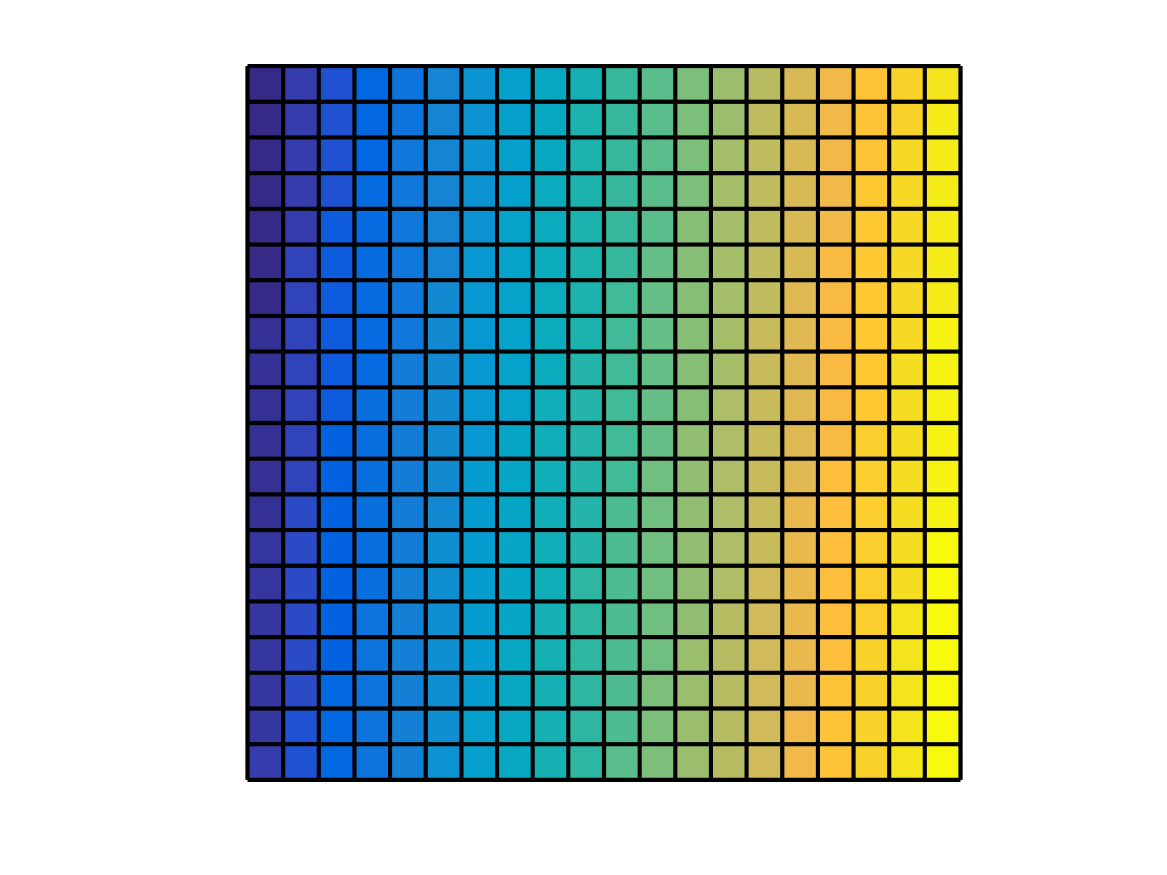
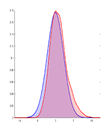
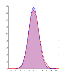
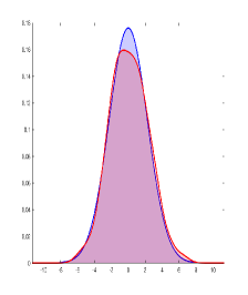
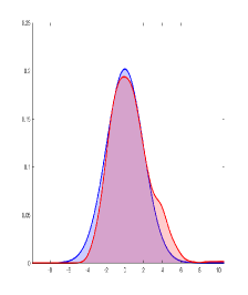
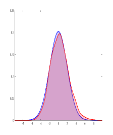
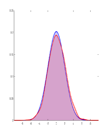
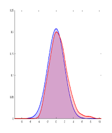
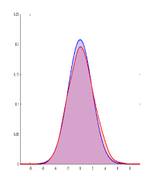
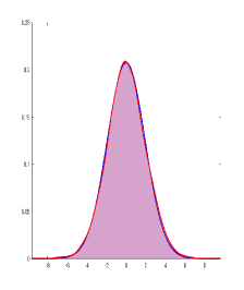
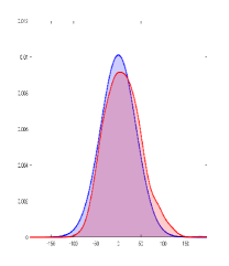
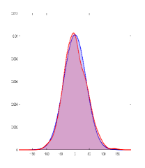
We generate empirical distributions (such that follows a multinomial distribution with parameter ) for different values of and grid size. In this way, we obtain realizations of , and we use a kernel density estimate (with a data-driven bandwidth) to compare the distribution of these realizations to the density of the Gaussian distribution . The results are reported in Figure 2 (grid ) and Figure 3 (grid ). It can be seen that the convergence of the empirical Sinkhorn loss to its asymptotic distribution () is relatively fast.
|
|
 |
 |
 |
|---|---|---|---|
|
|
 |
 |
 |
|
|
 |
 |
 |
|
|
 |
 |
 |
|---|---|---|---|
|
|
 |
 |
 |
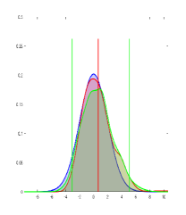
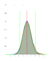
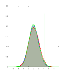
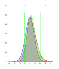
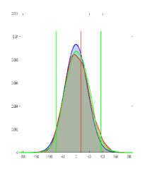
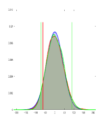
Let us now shed some light on the bootstrap procedure. The results on bootstrap experiments are reported in Figure 4. From the uniform distribution , we generate only one random distribution . The value of the realization is represented by the red vertical lines in Figure 4. Besides, we generate from , a sequence of bootstrap samples of random measures denoted by (such that follows a multinomial distribution with parameter ). We use again a kernel density estimate (with a data-driven bandwidth) to compare the distribution of to the distribution of displayed in Figure 2 and Figure 3. The green vertical lines in Figure 4 represent a confidence interval of level . The observation represented by the red vertical line is mostly located within this confidence interval, and the density estimated by bootstrap decently captures the shape of the non-asymptotic distribution of Sinkhorn losses.
|
Grid |
 |
 |
 |
|---|---|---|---|
|
Grid |
 |
 |
 |
4.1.2 Alternative - Two samples
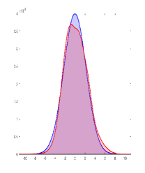
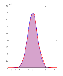
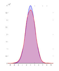
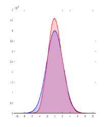
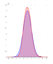
We consider the same setting as before, excepting that data are now both sampled from distributions and . Hence, we run experiments to obtain a kernel density estimation of the distribution of
that is compared to the density of the Gaussian variable
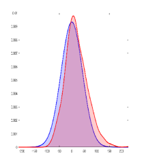
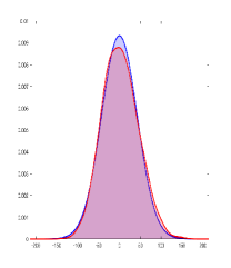
for different values of and . The results are reported in Figure 5. The convergence does not seem as good as in the one sample case, this must be due to the randomness coming from both and .
|
|
|
 |
 |
|---|---|---|---|
|
|
|
 |
 |
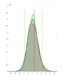
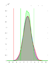
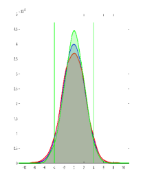
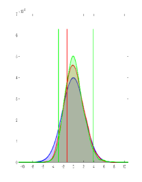
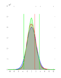
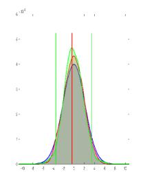
We also report in Figure 6 results on the consistency of the bootstrap procedure under the hypothesis with two samples. From the distributions and , we generate two random distributions and . The value of the realization is represented by the red vertical lines in Figure 6. Then, we generate from and , two sequences of bootstrap samples of random measures denoted by and . We use again a kernel density estimate (with a data-driven bandwith) to compare the green distribution of to the red distribution of displayed in Figure 6. The green vertical lines in Figure 6 represent a confidence interval of level . We can draw the same conclusion as in the one sample case. All these experiments thus perfectly illustrate the Theorem 2.7.
|
|
 |
 |
 |
|---|---|---|---|
|
|
 |
 |
 |
4.1.3 Hypothesis - One sample.
As in the previous cases, we consider to be the uniform distribution on a square grid. We recall that the distributional limit in the right hand side of (13) is the following mixture of random variables with chi-squared distribution of degree
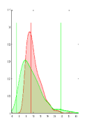
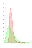
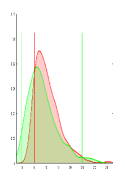
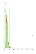
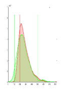
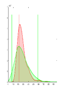
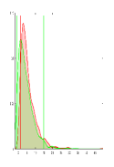
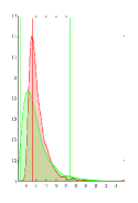
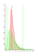
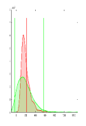
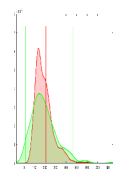
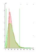
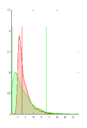
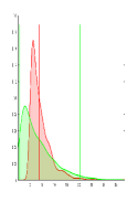
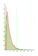
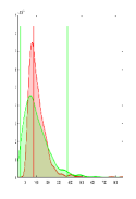
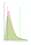
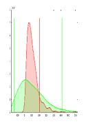
It appears to be difficult to compute the density of this distributional limit or to draw samples from it, since computing the Hessian matrix is a delicate task. We thus leave this problem open for future work, and only rely on the non-asymptotic distribution of . This justifies the use of the bootstrap procedure described in Section 3. We display the bootstrap statistic in Figure 7. The shape of the non-asymptotic density of (red curves in Figure 7) looks chi-squared distributed. In particular, it only takes positive values. The bootstrap distribution in green also recovers the most significant mass location of the red density.
|
|
 |
 |
 |
|
 |
 |
|
|
 |
 |
 |
|
 |
 |
|
|
 |
 |
 |
 |
 |
 |
| Grid | Grid | |||||
4.1.4 Hypothesis - Two samples.
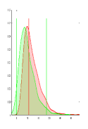
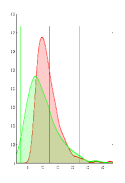
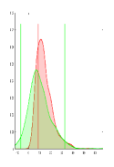
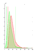
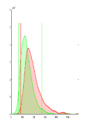
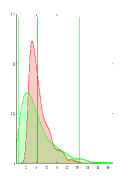
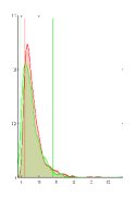
We still consider to be the uniform distribution on a square grid and we sample two measures from denoted . We compute the non-asymptotic distribution of which, from Theorem 2.9, must converge to with the eigenvalues of
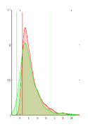
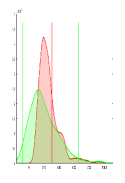
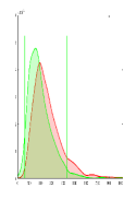
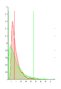
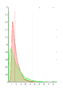
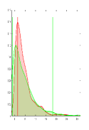
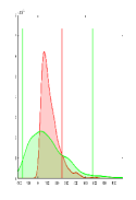
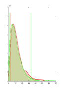
The results are displayed in red in Figure 8, together with the bootstrap distribution (in green) . We obtain similar results to the one sample case.
|
|
 |
 |
 |
|
 |
|
|
 |
 |
 |
|
 |
|
|
 |
 |
 |
 |
 |
| Grid | Grid | ||||
4.2 Estimation of test power using the bootstrap
One sample - distribution with linear trend and varying slope parameter.
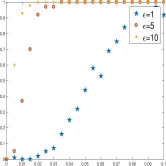
The consistency and usefulness of the bootstrap procedure is illustrated by studying the statistical power (that is ) of statistical tests (at level ) based on the empirical Sinkhorn loss. For this purpose, we choose to be uniform and to be a distribution with linear trend whose slope parameter is ranging from to on a grid. We assume that we observe a single realization of an empirical measure sampled from with . Then, we generate bootstrap samples of random measures from (with ), which allows the computation of the -value
This experiments is repeated 100 times, in order to estimate the power (at level ) of a test based on by comparing the resulting sequence of -values to the value . The results are reported in Figure 9 (left).
| = Relative entropy | = Entropy | ||
|
Test power |
 |
Test power |
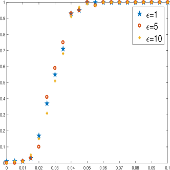 |
It can be seen that the resulting testing procedures are good discriminants for the three values of the regularization parameters that we considered. As soon as the slope increases then sufficiently differs from , and the probability of rejecting thus increases. We have also chosen to report results obtained with the Sinkhorn loss corresponding to optimal transport regularized by the entropy instead of the relative entropy (see Figure 9 (right)). Indeed, we remark that in the case of the relative entropy, the power of the test seems to highly depend on the value of . More precisely, for a fixed value of the slope parameter (or distribution ), the test power is larger as increases. On the other hand, when using the Sinkhorn loss computed with the entropy, the power of the test seems to be the same for any value of .
Remark 5.
The truly interesting property of the Sinkhorn loss over the Sinkhorn divergence is that in theory, for any , we will obtain a steady -dependent asymptotic distribution, and that any regularization allows us to perform test statistics. In practice, more regularization leads to a blending of information. More precisely, the entropy will spread the mass of the distributions, and in some points of the grid, the differences of masses between the two distributions can be the result of regularization. On the other hand, when very few observations are available, and that measures are sparsely distributed on the grid, a large will still allow to perform a statistical study.
5 Analysis of real data
We consider a dataset of colored images representing landscapes and foliage taken during Autumn (20 images) and Winter (17 images), see Figure 10 for examples. These images, provided by [24], are available at http://tabby.vision.mcgill.ca/html/welcome.html.
 |
 |
 |
 |
 |
 |
 |
 |
Each image is transformed into a color histogram on a three-dimensional grid (RGB colors) of size of equi-spaced points. We will denote by the autumn histograms and the winter histograms. To compute the cost matrix , we again use the squared Euclidean distance between the spatial integer locations .
5.1 Testing the hypothesis of equal color distribution between seasons
We first test the null hypothesis that the color distribution of the images in Autumn is the same as the color distribution of the images in Winter. To this end, we consider the mean histogram of the dataset for each season, that we denote
Notice that both and are discrete empirical measures admitting a zero mass for many locations .
We use the two samples testing procedure described previously, and a bootstrap approach to estimate the distribution of the test statistics
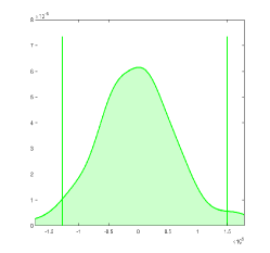
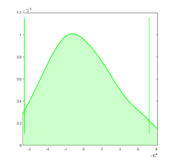
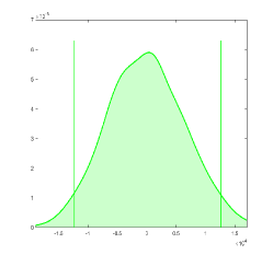
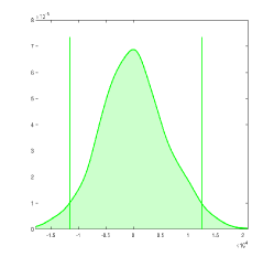
Notice also that and respectively correspond to the number of observations for the empirical Autumn distribution and the empirical Winter distribution , which is the total number of pixels times the number of images. Therefore, and . We report the results of the testing procedure for by displaying in Figure 11 an estimation of observations of the bootstrap statistic’s density
where and are respectively bootstrap samples of and , and are the optimal dual variables associated to in problem (3).
For , the value of is outside the support of this density, and the null hypothesis that the color distributions of images taken during Autumn and Winter are the same is thus rejected. In particular, the test statistic is equal to for and to for .
 |
 |
| (a) | (b) |
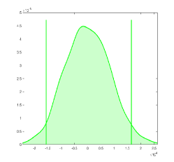
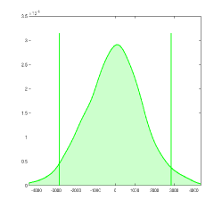
We also run the exact same experiments for a smaller grid (size ) and a higher number of observations (). The results are displayed in Figure 12. The distributions are much more centered around (we gain a factor ). However, we obtain the same conclusion as before, with a test statistic equal to for and for .
 |
 |
| (a) | (b) |
5.2 Testing the hypothesis of equal distribution when splitting the Autumn dataset
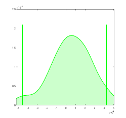
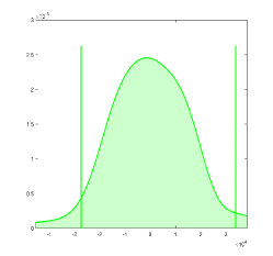
We propose now to investigate the equality of distributions within the same dataset of Autumn histograms. To this end, we arbitrarily split the Autumn dataset into two subsets of 10 images and we compute their mean distribution
for which . The procedure is then similar to the Autumn versus Winter case in Subsection 5.1, meaning that we sample bootstrap distributions and from respectively and . The results are displayed in Figure 13. We obtain similar results than in the two seasons case, the null hypothesis that both Autumn distributions follow the same law is thus rejected. On the other hand, the test statistics are smaller in this case as the histogram of color seems to be closer. Indeed, the quantity is equal to for and for .
 |
 |
| (a) | (b) |
.
Similarly to the Winter VS Autumn case, we also run the same Autumn VS Autumn experiments for a grid of size and observations. The results are displayed in Figure 14 for test statistics equal to for and for .
 |
 |
| (a) | (b) |
Remark 6.
For comparison purpose, we ran a test of homogeneity for testing the hypothesis of equal distributions of colors. The obtained test statistic in the Autumn vs Winter case is equal to , and in the Autumn splitting case to . Even if is indeed smaller than , the contrast between these two is weaker than with the Sinkhorn loss test.
6 Future works
As remarked in [32], there exists a vast literature for two-sample testing using univariate data. However, in a multivariate setting, it is difficult to consider that there exist standard methods to test the equality of two distributions. We thus intend to further investigate the benefits of the use of the empirical Sinkhorn loss to propose novel testing procedures able to compare multivariate distributions for real data analysis. A first perspective is to apply the methodology developed in this paper to more than two samples using the notion of smoothed Wasserstein barycenters (see e.g. [9] and references therein) for the analysis of variance of multiple and multivariate random measures (MANOVA). However, as pointed out in [9], a critical issue in this setting will be the choice of the regularization parameter , as it has a large influence on the shape of the estimated Wasserstein barycenter. Another interesting extension of the results presented in this paper would be to obtain the eigenvalues of the Hessian matrix of the Sinkhorn loss, in order to compute the distributional limit under the null hypothesis of equality of distributions.
References
- [1] M. Arjovsky, S. Chintala, and L. Bottou. Wasserstein GAN. arXiv preprint arXiv:1701.07875, 2017.
- [2] J. Bigot, E. Cazelles, and N. Papadakis. Data-driven regularization of wasserstein barycenters with an application to multivariate density registration. ArXiv e-prints, 1804.08962, 2018.
- [3] J. Bigot, R. Gouet, T. Klein, A. López, et al. Geodesic pca in the Wasserstein space by convex pca. Annales de l’Institut Henri Poincaré, Probabilités et Statistiques, 53(1):1–26, 2017.
- [4] S. Boyd and L. Vandenberghe. Convex optimization. Cambridge university press, 2004.
- [5] E. Cazelles, V. Seguy, J. Bigot, M. Cuturi, and N. Papadakis. Geodesic pca versus log-pca of histograms in the wasserstein space. SIAM Journal on Scientific Computing, 40(2):B429–B456, 2018.
- [6] Q. Chen and Z. Fang. Inference on functionals under first order degeneracy. SSRN, 2018.
- [7] M. Cuturi. Sinkhorn distances: Lightspeed computation of optimal transport. In Advances in Neural Information Processing Systems 26, pages 2292–2300. 2013.
- [8] M. Cuturi and A. Doucet. Fast computation of Wasserstein barycenters. In International Conference on Machine Learning 2014, JMLR W&CP, volume 32, pages 685–693, 2014.
- [9] M. Cuturi and G. Peyré. A smoothed dual approach for variational Wasserstein problems. SIAM Journal on Imaging Sciences, 9(1):320–343, 2016.
- [10] E. del Barrio, J. A. Cuesta-Albertos, C. Matrán, and J. M. Rodriguez-Rodriguez. Tests of goodness of fit based on the -Wasserstein distance. Ann. Statist., 27(4):1230–1239, 1999.
- [11] E. del Barrio, E. Giné, and F. Utzet. Asymptotics for functionals of the empirical quantile process, with applications to tests of fit based on weighted Wasserstein distances. Bernoulli, 11(1):131–189, 2005.
- [12] E. del Barrio and J.-M. Loubes. Central limit theorems for empirical transportation cost in general dimension. arXiv:1705.01299v1, 2017.
- [13] B. Efron and R. J. Tibshirani. An Introduction to the Bootstrap. Chapman & Hall, New York, 1993.
- [14] J. Feydy, T. Séjourné, F.-X. Vialard, S.-I. Amari, A. Trouvé, and G. Peyré. Interpolating between optimal transport and MMD using sinkhorn divergences. arXiv preprint arXiv:1810.08278, 2018.
- [15] G. Freitag and A. Munk. On Hadamard differentiability in -sample semiparametric models—with applications to the assessment of structural relationships. J. Multivariate Anal., 94(1):123–158, 2005.
- [16] C. Frogner, C. Zhang, H. Mobahi, M. Araya, and T. A. Poggio. Learning with a Wasserstein loss. In Advances in Neural Information Processing Systems, pages 2053–2061, 2015.
- [17] A. Genevay, L. Chizat, F. Bach, M. Cuturi, and G. Peyré. Sample complexity of sinkhorn divergences. arXiv preprint arXiv:1810.02733, 2018.
- [18] A. Genevay, M. Cuturi, G. Peyré, and F. Bach. Stochastic optimization for large-scale optimal transport. In D. D. Lee, U. V. Luxburg, I. Guyon, and R. Garnett, editors, Proc. NIPS’16, pages 3432–3440. Curran Associates, Inc., 2016.
- [19] A. Genevay, G. Peyré, and M. Cuturi. Sinkhorn-autodiff: Tractable Wasserstein learning of generative models. Preprint 1706.00292, Arxiv, 2017.
- [20] A. Gramfort, G. Peyré, and M. Cuturi. Fast optimal transport averaging of neuroimaging data. In International Conference on Information Processing in Medical Imaging, pages 261–272. Springer, 2015.
- [21] M. Klatt, C. Tameling, and A. Munk. Empirical regularized optimal transport: Statistical theory and applications. arXiv preprint arXiv:1810.09880, 2018.
- [22] G. Luise, A. Rudi, M. Pontil, and C. Ciliberto. Differential properties of Sinkhorn approximation for learning with Wasserstein distance. In Advances in Neural Information Processing Systems, pages 5859–5870, 2018.
- [23] X. Nguyen. Convergence of latent mixing measures in finite and infinite mixture models. Ann. Statist., 41(1):370–400, 02 2013.
- [24] A. Olmos and F. A. Kingdom. A biologically inspired algorithm for the recovery of shading and reflectance images. Perception, 33(12):1463–1473, 2004.
- [25] J. Rabin and N. Papadakis. Convex color image segmentation with optimal transport distances. In International Conference on Scale Space and Variational Methods in Computer Vision, pages 256–269. Springer, 2015.
- [26] A. Ramdas, N. G. Trillos, and M. Cuturi. On wasserstein two-sample testing and related families of nonparametric tests. Entropy, 19(2):47, 2017.
- [27] T. Rippl, A. Munk, and A. Sturm. Limit laws of the empirical Wasserstein distance: Gaussian distributions. J. Multivariate Anal., 151:90–109, 2016.
- [28] A. Rolet, M. Cuturi, and G. Peyré. Fast dictionary learning with a smoothed Wasserstein loss. In Proc. International Conference on Artificial Intelligence and Statistics (AISTATS), 2016.
- [29] M. A. Schmitz, M. Heitz, N. Bonneel, F. M. N. Mboula, D. Coeurjolly, M. Cuturi, G. Peyré, and J.-L. Starck. Wasserstein dictionary learning: Optimal transport-based unsupervised non-linear dictionary learning. arXiv preprint arXiv:1708.01955, 2017.
- [30] V. Seguy and M. Cuturi. Principal geodesic analysis for probability measures under the optimal transport metric. In C. Cortes, N. Lawrence, D. Lee, M. Sugiyama, and R. Garnett, editors, Advances in Neural Information Processing Systems 28, pages 3294–3302. Curran Associates, Inc., 2015.
- [31] J. Solomon, F. de Goes, G. Peyré, M. Cuturi, A. Butscher, A. Nguyen, T. Du, and L. Guibas. Convolutional wasserstein distances: Efficient optimal transportation on geometric domains. In ACM Transactions on Graphics (SIGGRAPH’15), 2015.
- [32] M. Sommerfeld and A. Munk. Inference for empirical wasserstein distances on finite spaces. Journal of the Royal Statistical Society: Series B (Statistical Methodology), 2016.
- [33] J. Sourati, M. Akcakaya, T. K. Leen, D. Erdogmus, and J. G. Dy. Asymptotic analysis of objectives based on fisher information in active learning. Journal of Machine Learning Research, 18(34):1–41, 2017.
- [34] A. Thibault, L. Chizat, C. Dossal, and N. Papadakis. Overrelaxed sinkhorn-knopp algorithm for regularized optimal transport. arXiv preprint arXiv:1711.01851, 2017.
- [35] A. W. Van Der Vaart and J. A. Wellner. Weak convergence and empirical processes. Springer, 1996.
- [36] C. Villani. Topics in optimal transportation, volume 58 of Graduate Studies in Mathematics. American Mathematical Society, 2003.
- [37] L. Wasserman. All of statistics: a concise course in statistical inference. Springer Science & Business Media, 2011.
- [38] A. G. Wilson. The use of entropy maximising models, in the theory of trip distribution, mode split and route split. Journal of Transport Economics and Policy, pages 108–126, 1969.
- [39] J. Ye, P. Wu, J. Z. Wang, and J. Li. Fast discrete distribution clustering using Wasserstein barycenter with sparse support. IEEE Trans. Signal Processing, 65(9):2317–2332, 2017.
- [40] C. Zalinescu. Convex analysis in general vector spaces. World Scientific, 2002.