A Gamut Mapping Framework
for Color-Accurate Reproduction of HDR Images

Abstract

Few tone mapping operators (TMOs) take color management into consideration, limiting compression to luminance values only. This may lead to changes in image chroma and hues which are typically managed with a post-processing step. However, current post-processing techniques for tone reproduction do not explicitly consider the target display gamut. Gamut mapping on the other hand, deals with mapping images from one color gamut to another, usually smaller, gamut but has traditionally focused on smaller scale, chromatic changes. In this context, we present a novel gamut and tone management framework for color-accurate reproduction of high dynamic range (HDR) images, which is conceptually and computationally simple, parameter-free, and compatible with existing TMOs. In the CIE $LCh$ color space, we compress chroma to fit the gamut of the output color space. This prevents hue and luminance shifts while taking gamut boundaries into consideration. We also propose a compatible lightness compression scheme that minimizes the number of color space conversions. Our results show that our gamut management method effectively compresses the chroma of tone mapped images, respecting the target gamut and without reducing image quality.

I Introduction

High dynamic range (HDR) imaging consists of tools and techniques to capture, store, transmit and display images with significantly higher fidelity than can be achieved with conventional imaging techniques. An important aspect of HDR imaging involves the reproduction of images on conventional displays. As in this case the dynamic range of the image can be much higher than the display device can accommodate, dynamic range reduction techniques need to be employed [1, 2].

In many cases, tone reproduction techniques focus on range compression along the luminance dimension, either leaving chromaticities unaltered, or treating color management as a separate problem [3, 4, 5]. In the latter case, algorithms focus on correcting or improving the appearance of the tonemapped image. Some HDR color appearance models do integrate color and luminance management, for the purpose of predicting the human visual response to a stimulus [6, 7]. Such algorithms can be used successfully as display algorithms, albeit still without appropriate gamut management.

To our knowledge, none of the existing algorithms take the target color gamut into consideration and as a result often produce pixel values that cannot be correctly represented or displayed. Our method aims to combine the color correction step often necessary after tone mapping with gamut management into an integrated HDR gamut management framework that handles both lightness and chroma compression, while limiting as much as possible hue shifts and luminance distortion.

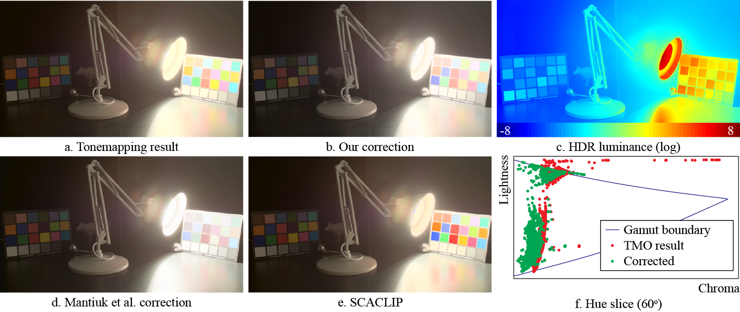
Figure 1: An HDR image, shown in (c) in false-color, was tone mapped using the Photographic operator [8] (a) and processed with our framework (b), a color correction solution [4] (d) and a gamut mapping solution [9] (e). Although the tone mapping process has successfully compressed the luminance of the image, it has led to an over-saturated appearance and out-of-gamut pixels (f). Our method corrects both issues, while alternative solutions only handle one of the two.

There are good reasons why these two dimensions should be treated in conjunction. First, human vision does not treat colorfulness separately from luminance values, as evidenced by the Hunt effect. In essence, lighter objects are seen as more colorful, and vice-versa. In the context of dynamic range management, this means that compression of luminances should be accompanied by a corresponding adjustment of chroma. Additionally, current consumer display trends are pushing towards a combined increase in gamut and dynamic range, necessitating algorithms that can manage both of these aspects in conjunction.

Second, color spaces are three dimensional, bounded by their gamut [10]. The gamut spanned by the pixels in an image may not be matched to that of the target display. In such cases, gamut mapping involves compensating for differences in size, shape and location between the image and display gamuts. This constitutes a mapping from one three-dimensional shape to another. As the overlap between gamuts is typically large in conventional gamut mapping scenarios, such algorithms aim to find a trade-off between moving out-of-gamut pixels inside the target gamut, while pixels that are already inside the target gamut are left alone as much as possible.

On the other hand, one-dimensional luminance adjustment, as achieved by many tone reproduction operators, may create pixels that lie outside the target display’s gamut (see Figure 1f) along the chroma channel. These pixels are either typically not managed or treated with naïve approaches [3] that tend to over-saturate as shown in Figure 1a.

Our novel gamut mapping framework integrates tone mapping with gamut mapping, correcting the colors after dynamic range compression, while ensuring that images fit within the target gamut. It does not require calibrated input and is parameter-free. We accomplish this by transforming the original HDR image into the CIE $L^{*}C^{*}h^{*}$ color space, and then compressing both the lightness and chroma channels as customary in gamut mapping algorithms. The lightness channel can be compressed with any existing tone mapping operator, or a scheme similar to our chroma compression can be applied to lightness as well.

Side-bar: Gamut Mapping

Given a color space, a gamut for a device or medium can be thought of as a subspace within the color space, containing the colors that can be reproduced by that device. A new color that is outside the gamut, cannot be accurately reproduced by the device. To define how colors outside this gamut should be treated or mapped to the displayable color subset, gamut mapping techniques may be employed. Gamut mapping techniques can be categorized as global and spatial. Global techniques can be further classified as clipping and compression based approaches. Clipping only changes the colors that are located outside of the destination gamut by clamping them to the boundaries of the destination gamut [10]. Although it has the advantage of preserving within-gamut colors, it is only a viable solution if the difference between the two gamuts is small. Compression, on the other hand, changes all the colors of the input gamut to be adjusted into the destination gamut [10]. Different types of compression functions have been proposed such as linear, piecewise linear, and sigmoidal. Compression is typically performed on both lightness and chroma components. In contrast to the global approaches, spatial gamut mapping attempts to preserve local information. These methods will map similar out-of-gamut colors to the same color if they are spatially distant in the image, but to distinct colors if they share an edge. Our work aims to extend existing work on gamut mapping for low dynamic range, proposing a gamut mapping management framework to work directly with HDR input data. This can be either integrated into existing TMOs or be a fully stand alone solution with its own lightness compression technique for (HDR) luminance values.

II Related Work

Reproduction of visual content on devices of different gamuts is typically divided into two categories, namely gamut mapping and tone mapping. Traditionally the first class of techniques deals with mapping the color gamut between devices, attempting to produce the most accurate reproduction of colors possible given the restrictions of a given device or medium [10]. Tone mapping, on the other hand, is primarily concerned with compressing the luminance range of an HDR image or video such that the media can be visualized on a low dynamic range (LDR) display device [1, 2].

In contrast to tone or gamut mapping, color appearance models (CAMs) predict human visual perception of patches of color and images. They consider parameters relating to the scene and viewing environment and as such require accurate measurements as input. These methods can accurately reproduce the appearance of an image in different devices and viewing conditions, but do not take gamut boundary issues into consideration.

Although both tone mapping and gamut mapping research aim to reproduce images on devices of more limited capabilities, they have remained largely disconnected areas. In this work, we bring together these two fields (see side-bars) in a novel gamut management technique that can successfully compress the chromaticities of high dynamic range (HDR) images so that they correctly match the compression applied by any given tone mapping operator.

Side-bar: Tone Mapping

Tone mapping is typically used to prepare HDR images for display on LDR display devices. While tone mapping can be considered a form of gamut mapping, there are important differences. First, tone mapping is generally employed when the dynamic range of the input image is vastly higher than the dynamic range of the display device. Second, tone mapping is generally concerned with compressing luminances, while gamut mapping is concerned with compressing perceptual attributes of lightness and chroma. As such, it is possible that a tone mapped image will contain out-of-gamut colors, which are clipped to gamut boundaries in an uncontrolled manner. An additional concern when tone mapping the luminance channel only is that images tend to acquire an over-saturated appearance either globally or locally, as shown in Figure 1a. Appearance aspects such as saturation and colorfulness of an image or image patch depend both on the chromatic information and the image luminance. Thus, to fix these color distortions, most TMOs are augmented with a post processing step that desaturates the image by means of a manually controlled parameter [3], while psychophysical studies have linked this saturation parameter to the amount of contrast correction computed from the global tone mapping curve [4]. Alternatively, the amount of (de-)saturation can be computed by comparing the original HDR input to the tone mapped result [5]. Although these methods can improve the appearance of the tone mapped image, they are not able to consider the gamut boundaries of the target medium.

III HDR Gamut Management Framework

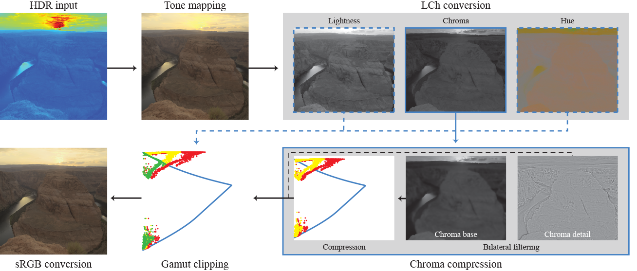
Figure 2: Overview of our framework. The input HDR image (here illustrated with a heat-map of luminance values) is first tone mapped and then converted to the $LCh$ color space. Chroma values are then filtered using the bilateral filter and the base layer is compressed. Finally, a gamut clipping step ensures that the compressed chroma and lightness values fit within the target gamut while minimizing appearance changes. (Red: input, Yellow: Chroma compressed, Green: Final result)

Our framework incorporates tone mapping, chroma correction, and gamut management to process an HDR image for a given output gamut. In this section, we will discuss the components of our solution in the context of existing dynamic range compression algorithms. The workflow is shown in Figure 2.

The input to our pipeline is an HDR image $I$ given in linear XYZ coordinates. First, the luminance channel of the image, denoted $I(L)$, is compressed using any existing tone mapping operator (TMO). The chroma channel $I(C)$ of the resulting image is then corrected with our chroma compression algorithm to correct for unwanted saturation due to the tone mapping process. Finally, image chroma and luminance values $I(C,L)$ are processed with a gamut management step to ensure that all pixels fit within the target gamut boundaries, denoted $G(C,L)$, while minimizing appearance changes in the image.

III-A Luminance Compression

As we want to ensure that our chroma compression and subsequent gamut management steps correct any issues that the tone mapping process may have caused, the first component of our framework is the luminance compression. Our framework has been designed to easily integrate with existing TMOs and in the following we describe the steps for integrating the commonly used Photographic operator [8]:

1. The input HDR is first converted to the color space expected by the TMO (in this case $Yxy$).

2. The tone mapping curve is applied on the luminance Y, obtaining the compressed value $Y_{c}$. Both local and global algorithms can be applied at this point as our framework poses no restrictions on the type of processing.

3. The compressed luminance is inserted into the image and the result is converted back to the $XYZ$ color space.

4. Finally, the tone mapped image $I$ is normalized, such that the maximum $Y$ value is 100, to allow for further processing. In the case of the Photographic operator, output luminance values are between 0 and 1, and as such require scaling to the range expected by the color space used in further processing. This is discussed further in the following section.

Although this process allows for flexibility in the choice of luminance compression, it comes at the cost of increased computational complexity due to additional color space transforms, as existing TMOs are not necessarily designed to operate in a color space that enables gamut manipulations. As an alternative solution, we have designed a compression solution that follows a similar scheme to our chroma compression method, which is described in the side-bar “Lightness Compression using Cusp Alignment”.

III-B Gamut Boundary Computation

Our algorithm relies on the idea that to avoid undesired shifts in chroma and hue, as well as to avoid uncontrolled clipping for out-of-gamut colors, one should work in a perceptually decorrelated color space where these components are separated. A natural choice for this is the CIE $L^{*}C^{*}h^{*}$ color space, which is the cylindrical representation of CIE $L^{*}a^{*}b^{*}$ . These two color spaces are commonly used in traditional gamut mapping algorithms [10].

To determine the correct compression amount and to assess whether a given pixel can fit within the output gamut, we need to know the boundaries of that gamut. In this paper, we assume that the target gamut is sRGB and as such use a D65 white point when converting to LAB. Our algorithm, however, can accommodate any alternative gamut and corresponding white point. The source or input gamut is the set of colors of the input HDR image. Computing the boundaries of both gamuts we have followed the methodology described in [10] to obtain the boundaries of the sRGB gamut in LCh coordinates, which take the form of a triangular cusp along the chroma-lightness plane for each hue value. Figure 3 shows the extreme differences between the source (red) and the target (white) gamuts that may occur in HDR imaging. Between source and target, the differences in both lightness and chroma channels exceed a factor of 10.

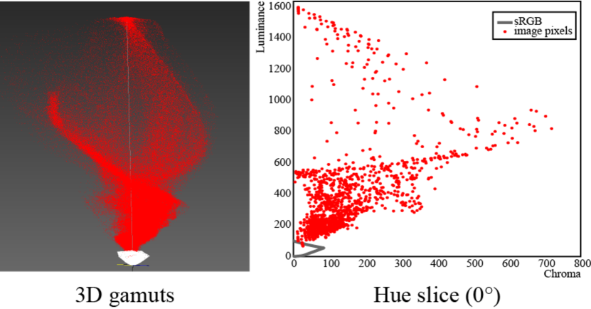
Figure 3: Boundaries of the source gamut (input HDR image - red) and the target gamut (sRGB color space - white).

III-C Chroma Compression

When considering HDR imagery, a large number of pixel values may be outside the destination gamut in terms of chroma, generating unwanted hue shifts if clipped in an uncontrolled manner.

Additionally, it has been shown that tone compression along the luminance dimension tends to create an over-saturated appearance in images. This is illustrated in Figure 1. To correct these issues, we are proposing two methods that compress the chroma values $I(C)$ in the image in a content-dependent manner.

III-C1 Hue-Specific Method

This method compresses the chroma values $I(C)$ in the image using a two step process. The first step for our algorithm is to determine a scaling factor $R_{h}$ for each hue value $h=\left[1^{\circ}\ldots 360^{\circ}\right]$, leading to a vector R. To achieve that, we scale the gamut boundaries $G_{h}(C,L)$ until they enclose all pixels within that hue slice. Formally, we initialize the scaling factor for a hue slice $R_{h,0}=1$. If there are pixels that are out of gamut for that hue slice, at each iteration step $i$, we increment the scale factor $R_{h,i}$ and scale the gamut boundaries as follows:

$$R_{h,i} =R_{h,i-1}+d$$ (1)

$$G_{h,i}(C,L) =\left[\begin{array}[]{cc}R_{h,i}&0\\ 0&R_{h,i}\end{array}\right]G_{h}(C,L),$$ (4)

where the increment $d$ is set to a small value (in all the results in the paper $d=0.1$). This process is illustrated in Figure 4a.

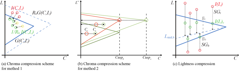
Figure 4: Compression scheme presented in this paper for the (a) Chroma compression (Hue-Specific), (b) Chroma compression (Global) and (c) Lightness compression.

While this scaling factor could be applied to the image values directly to obtain a within-gamut result, in practice, using the full chroma range of the source gamut would likely result in extreme compression due to a few outlying pixels with extremely high chroma. This is a common problem in luminance compression, where some extremely bright highlights may lead to an over-compressed result and is usually countered by compressing according to a percentile of the range of values. In the case of chroma, if the compression takes into account such pixels, the resulting image may be too desaturated.

To avoid this undesirable effect, we use a percentile of the chroma range when computing R. We have found that the percentile value required is content dependent—if the pixels that require clipping are spread over the image, then a more aggressive percentile value may be selected. If, however, the out-of-gamut pixels are concentrated in a small number of regions, a more gentle approach is necessary to ensure that no artifacts are created. In practice, we determine the spread of out-of-gamut pixels by computing the number of connected regions that they belong to and comparing them to the number of pixels contained within them. We have found that a ratio less than 0.01 suggests that the out-of-gamut pixels are within a few connected regions and therefore further clipping may lead to artifacts.

To be able to keep fine details without smoothing edges, the chroma channel of the image $I(C)$ is first processed with the bilateral filter ($\sigma_{s}=0.2\max(I_{width},I_{height}),\sigma_{r}=0.05\max(I(C))$) obtaining a base layer $I(C)_{\textrm{base}}$, which is used in the above computation. Either division or subtraction can be used to separate the base and detail layers. We have verified that both methods are leading to similar results so as we have decided to use the division method for producing the detail layer $I(C)_{\textrm{detail}}=I(C)/I(C)_{\textrm{base}}$. Figure 6 (left) shows how fine details are preserved, i.e. doors of the drawer and borders of the sink, when bilateral filtering is applied to the chroma channel.

Even with these measures, small variations in content between adjacent hue slices may lead occasionally to discontinuities in the final image if $R_{h}$ is applied directly to each slice. Smoothing the scaling vector R, to R’, will eliminate these discontinuities. To achieve this, one can use different type of smoothing functions. We have used four different smoothing functions: lbox (averaging box), loess (locally weighted regression), rloess (robust locally weighted regression) and sgolay (Savitzky– Golay). We find that the four smoothing functions produce results of similar quality, so the simpler and more computationally efficient function can be used in our framework (lbox). During the smoothing step, the circular nature of hues is taken into account. This avoids the creation of boundaries between the hue angles of 359 and 0.

Finally, image chroma within each hue slice $I(C)_{\textrm{base},h}$ is scaled as:

$$I(C)^{\prime}_{\textrm{base},h}=\frac{1}{R^{\prime}_{h}}I(C)_{\textrm{base},h}$$ (5)

and the detail is re-injected to obtain the chroma-compressed image $I(C)^{\prime}=I(C)^{\prime}_{\textrm{base}}\times I(C)_{\textrm{detail}}$, where $\times$ indicates an element-wise multiplication. Note that the reciprocal R’ needs to be used for the final compression as R was initially computed to expand the gamut boundaries until they enclosed all pixels

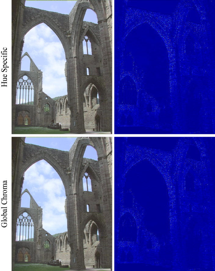
Figure 5: Results using the two chroma compression methods proposed in this paper and their hue differences maps.

III-C2 Global Method

The hue-specific method described in the previous section can successfully compress chroma, therefore maximizing the use of the available gamut. This however comes at the cost of increased computational complexity. At the same time, we may observe that the dynamic range of the chroma channel is not extremely high, when compared with the dynamic range of the display gamut. This suggests that a linear compression scheme may produce good results as shown in the hue difference maps of Figure 5. As such, we propose an alternative but simpler method based on similar premises. We envisage that the hue-specific method would be suitable for a post-production pipeline where accuracy is the primary goal, while the linear method described in this section would be better suited on the display-side of an imaging pipeline, where computational resources are limited.

The global method is illustrated in Figure 4(b). In this figure, the light and dark green triangles represent the source and destination gamuts respectively for a fixed hue angle. Our goal is to align the two chroma cusps while maintaining lightness and hue. In the figure, this would produce the red triangle which represents the compressed gamut.

Chroma compression is still applied on each hue angle from $0^{\circ}$ to $359^{\circ}$. Instead of using different amounts of chroma compression for each hue however, which requires additional computations, we compute the minimum of the cusps ratios across all hues. This value corresponds to the maximum necessary compression.

Similar to the hue-specific method, chroma compression is applied to the base layer of the chroma channel. We compress the source chroma $I(C)_{\textrm{base},h}$ to yield the compressed chroma $I(C)^{\prime}_{\textrm{base},h}$ as follows:

$$I(C)^{\prime}_{\textrm{base},h}=I(C)_{\textrm{base},h}\min_{h\in[0^{\circ},359^{\circ}]}\left[\frac{\textrm{Cusp}_{d,h}}{\textrm{Cusp}_{s,h}}\right].$$ (6)

where it is noted that this is only a compression when $\min\left[\textrm{Cusp}_{d,h}/\textrm{Cusp}_{s,h}\right]<1$.

We may face similar issues as in the hue-specific method when using the full chroma range of the source gamut. This will produce extremely compressed chroma results in some cases due to the use of a few outlying pixels with extremely high chroma values. To avoid this problem, we have adopted the same percentile approach used for the first method. This solution avoids over-compression but requires an additional step for managing the few pixels that may remain outside the gamut boundary, which is discussed in the next section.

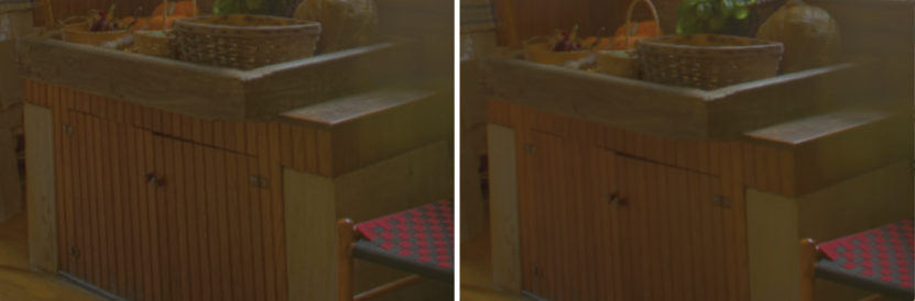
Figure 6: Results (left) with and (right) without bilateral filtering decomposition.

III-D Gamut Clipping

Since chroma and lightness values are so far processed independently, we cannot guarantee that all pixels will be within the target gamut boundaries. This is shown in Figure 7, during tone mapping pixels are compressed through the lightness direction. However, pixels are guarantee to have maximum lightness values equal to 100 nits, but may still be outside of the target gamut boundaries (red pixels). Applying chroma compression does not solve this problem (yellow pixels). To have all pixels within the target gamut boundaries, without further modifying pixels already in-gamut, a clipping step is employed. As image pixels may be out of gamut both in terms of chroma and lightness, as shown in Figure 7, pixel values need to be clipped along both dimensions creating a trade-off between changes in lightness or in chroma for each pixel.

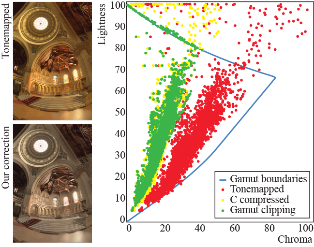
Figure 7: Here we plot the chroma values (x-axis) of pixels within a hue slice ($h=60^{\circ}$) against their lightness values (y-axis). After tone mapping the lightness channel of the image, many pixels (shown in red) are still outside the gamut boundaries. Scaling the chroma channel moves pixels closer to the gamut boundaries (yellow), while the last step in our framework ensures that pixels are mapped to values within the target gamut (green). The resulting image after tone mapping is shown at the top left and after our correction and clipping step at the bottom left.

Although many proposals exist for defining the clipping line along which pixels should move, they are designed for scenarios where the input and target gamuts differ in terms of chromatic primaries used rather than luminance range. In our specific case however, we have found that most out-of-gamut pixels tend to be bright, highly chromatic pixels (red pixels outside the gamut boundaries in Figure 7).

Because of the narrowing of the cusp near high-L values, a delicate balance between chroma and lightness adjustments is necessary to ensure that the resulting image appearance does not change. This is demonstrated in Figure 8: the area around the sun either desaturates completely as the lightness values are near the peak of the cusp (Figure 8a) or it looks too saturated because its lightness is decreased with no corresponding chroma changes (Figure 8b).

Instead, we propose a middle-ground between these two extremes. In a given hue slice, for a pixel $p\in I^{\prime}$ we determine a point along the gamut boundaries $p_{\textrm{clipC}}$ such that $p_{\textrm{clipC}}(C)\in G(C)$ and $p_{\textrm{clipC}}(L)=p(L)$. Similarly, a value $p_{\textrm{clipL}}$ is determined, where $p_{\textrm{clipL}}(C)$ remains unchanged and $p(L)_{\textrm{clipL}}$ moves to the gamut boundary. Once these two points have been computed, linear interpolation is performed to map the out of gamut pixel to the corresponding gamut boundary of the destination gamut.

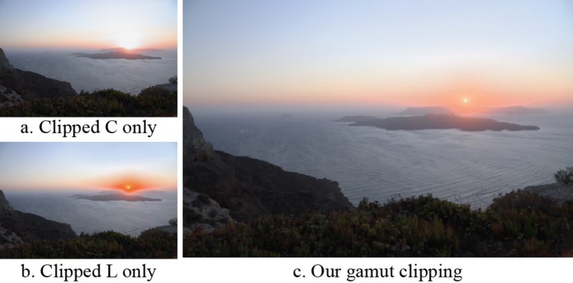
Figure 8: Three different clipping solutions were used to process the same image. Since most of the out-of-gamut pixels reside in the top right corner of the cusp, clipping along only the chroma direction (a) severely desaturates these pixels. In contrast, clipping only along the lightness direction (b) leads to an unnatural, oversaturated appearance. The result of our interpolated solution is shown in (c), where the image has maintained a natural appearance while all pixels fit within the gamut boundaries.

Side-bar: Lightness Compression using Cusp Alignment

Although the main goal of this paper is to present our framework for managing the gamut mismatches that tone mapping causes in terms of the resulting image chroma, we have found that our approach can be directly extended to compress the lightness channel, leading to an integrated luminance and color gamut management framework and minimizing the number of color space conversions necessary. To compress the lightness channel $I(L)$, we process each hue slice separately similar to the process described in Section III-C. The compression scheme is depicted in Figure 4(c). Specifically, we follow these steps for each hue slice: (1) We first find the global parameters that express the maximum vertical (lightness) distance from the destination gamut. The distance at the top is named $SG_{t}$ and at the bottom $SG_{b}$ (see Figure 4 (c)). Both values are set to $0$ when all pixels of the source gamut are already inside the destination gamut. (2) The “middle” line $L_{\textrm{mid}}$ is computed for the cusp of each hue slice by: $$L_{\textrm{mid}}=g_{b}+(g_{t}-g_{b})\frac{SG_{b}}{(SG_{t}+SG_{b})},$$ (7) where $g_{b}$ and $g_{t}$ are the bottom and the top values of the destination gamut. Note that this equation shifts the middle line toward $g_{b}$ for large $SG_{t}$, effectively compressing more of the image and toward $g_{t}$ for large $SG_{b}$, in which case more pixels are scaled linearly. That is, it adaptively determines a threshold that separates the source gamut into two regions that can be thought of as “light” and “dark”, with a magnitude for each determined by the ratio $SG_{t}$:$SG_{b}$. We treat each of these regions separately. (3) In the “light” region, i.e. for points above the $L_{\textrm{mid}}$, the lightness is compressed as follows: $\displaystyle I(L)_{c}$ $\displaystyle=a_{t}+b_{t}*F(I(L)-L_{\textrm{mid}}).$ (8) The compression factors $a_{t}$ and $b_{t}$ are computed by $a_{t}=L_{\textrm{mid}}$ and $b_{t}=\frac{(1-w)(g_{t}-L_{\textrm{mid}})+w(100-L_{\textrm{mid}})}{N}$, respectively, where the normalization factor is $N=F(g_{t}+SG_{t}-L_{\textrm{mid}})$ and the weight $w$ is computed as $w=\frac{I(C)}{I(C)+\max(G(C))}$. Here $F(x)$ represents a non-linear compression function, which is applied to pixels above $L_{\textrm{mid}}$. This could be any desired tone curve, including for instance sigmoidal compression or basic compressive functions such as roots and logarithms. Note that Equation 8 compresses the range $[L_{\textrm{mid}},g_{t}+SG_{t}]$ to $[L_{\textrm{mid}},b_{t}N+L_{\textrm{mid}}]$. Consequently, pixels with really high chroma and lightness may be mapped above the gamut boundary, and therefore clipped in the following stage of our framework. Since the clipping process takes into account both $C$ and $L$ values, this ensures that such pixels will still remain bright in the final image. (4) For points below $L_{\textrm{mid}}$, linear compression is used: $$I(L)_{c}=a_{b}+b_{b}*(I(L)-L_{\textrm{mid}}).$$ (9) In this case, the parameters are computed as $a_{b}=g_{b}$ and $b_{b}=\frac{L_{\textrm{mid}}-g_{b}}{L_{\textrm{mid}}}$. Note that here we compress the range $[g_{b}-SG_{b},L_{\textrm{mid}}]$ to $[g_{b},L_{\textrm{mid}}]$. Our method effectively corresponds to a non-linear compression with a linear ramp in dark areas. Such a behavior is commonly used in film. In our case however, the gamut of the image is explicitly considered to guide this compression scheme. To improve visibility in dark regions, we adopt a similar technique used for the chroma compression by making use of a percentile and processing $I(L)$ with the bilateral filter before compression. An example of our tone curve for the base layer compared with other global TMOs is shown in Figure 9 [11, 12, 8]. Figure 9: Tone curves making use of (blue) our method (HDR Gamut) and three global TMOs - (red) Ashikmin [12] - (green) Drago et al [11] - (black) Reinhard et al. [8].

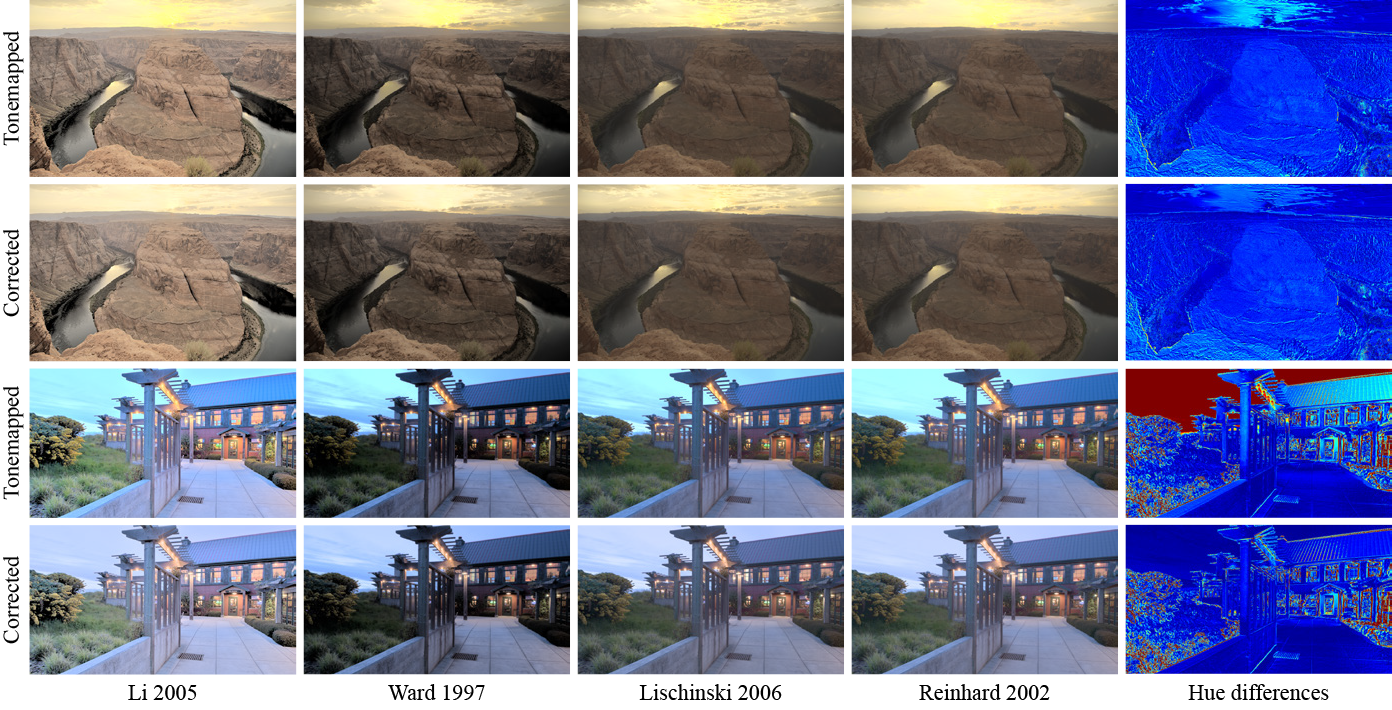
Figure 10: Shown here are HDR images that were processed with the TMOs by Li et al., Ward et al., Lischinski et al., and Reinhard et al. The output of the TMOs with no further processing is shown at the top, while the bottom row shows the output of the TMOs integrated with our chroma compression technique. The rightmost column shows hue differences between the TMO output and the HDR original (top) and between our corrected result and the HDR original (bottom) for the TMO by Reinhard et al. Hue differences are reduced for other TMOs as well.

IV Results

We have validated our technique using several challenging HDR images, demonstrating its benefits over existing techniques, including gamut mapping solutions, color correction methods, and color appearance models (CAMs). Additionally, we show the flexibility of our approach to be used with existing TMOs, without degradation of the details or introducing unwanted artifacts. We evaluate the quality of our reproduction by measuring hue changes as well as through a psychophysical study comparing our chroma compression method with alternative techniques. All the results shown in this section assume sRGB primaries for both input and output. They have been gamma corrected using the sRGB gamma correction equation, and use the chroma compression method specified in Section III-C1.

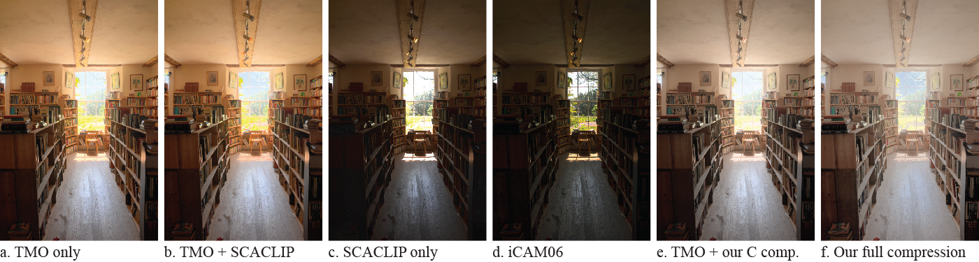
Figure 11: An HDR image is shown after being processed with different compression solutions. (a) Tone mapped with the Photographic operator [8] (b) Tone mapped and then processed with the SCACLIP gamut mapping method [9] (c) Processed only with SCACLIP (d) Processed with iCAM06 [6] (e) Tone mapped and processed with our chroma correction step (f) Processed with our integrated lightness and chroma compression.

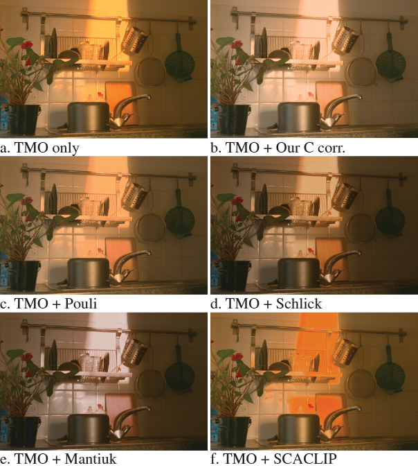
Figure 12: The tone mapped image (a) was corrected using our method (b) as well as existing color correction solutions (c,d and e) [5, 3, 4].These methods aim to correct the over-saturated appearance resulting from many tone mapping solutions and operate as a post-process on the image, without any gamut considerations. The result of combining the SCACLIP gamut mapping method with a TMO is shown in (f).

Our approach can handle challenging images, producing natural results that preserve details in the image while fitting within the target output gamut. Figure 1 shows the result of processing such an image with our framework as well as with other techniques (see supplemental material for more images). Existing tone mapping techniques (in this case the Photographic operator [8]) can effectively compress the luminance in the image but lead to an oversaturated appearance, with many pixels still out-of-gamut (e.g., colors of the macbeth color checker).

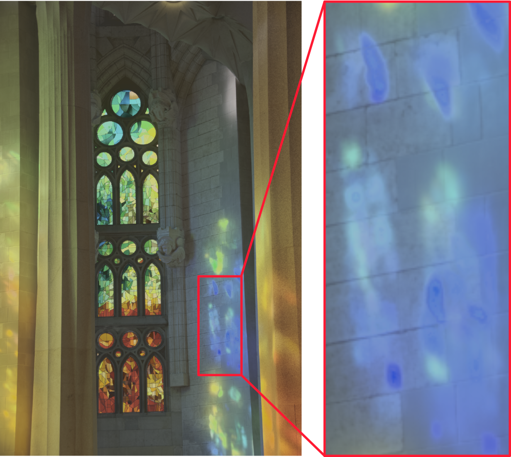
Figure 13: An example showing that the SCACLIP gamut mapping method [9], integrated with an existing TMO [8] may introduce artifacts.

Although a gamut mapping solution such as SCACLIP [9] can control this issue by moving pixels within the gamut boundaries, it may amplify the appearance of over-saturation (Figure 1e) or it introduces artifacts as shown in §Figure 13. At the same time, although such a gamut mapping approach modifies lightness values, it cannot sufficiently compress the extreme dynamic range of this image if used alone as seen in Figure 11c.

In contrast, our framework combines the advantages of tone mapping and gamut mapping (Figure 1b and Figure 11e). Our solution also allows for flexibility in the choice of compressive function: different functions can lead to different image appearances as shown in Figure 10. Despite the very different tone mapping styles, our chroma correction leads to a consistent treatment of colors in the images.

Finally, Figure 12 shows a comparison between our chroma correction and other color correction solutions that are typically applied as a post-process to tone compression as well as the result of SCACLIP after tonemapping. Note that the three color correction methods shown do not consider the gamut boundaries and therefore may lead to out-of-gamut pixels (in our experiments, we found that this often includes more than $10\%$ of the image pixels).

IV-A Hue differences

Ideally, compressing separately lightness and chroma at fixed hue should not affect hues. To assess whether our algorithm achieves that, we have evaluated our results using color difference metrics. Typically, color differences are computed using $\Delta E$ color difference metrics, which take into account both luminance and chromatic differences. In our case, a metric capable of separating luminance, chroma, and hue is necessary as we are only interested in preserving the hue while luminance and chroma are being compressed.

Although color difference measurements are commonly performed in the LAB color space, it is known that LAB is not hue-linear across all hues. Instead, we use an optimized $I^{\prime}P^{\prime}T^{\prime}$ space for color difference comparisons [13]. This space is scaled and rotated with respect to $IPT$ such that color differences in this new space are directly comparable with other color difference metrics, while preserving hue linearity.

In $I^{\prime}P^{\prime}T^{\prime}$, a cylindrical space is then computed, where lightness $\Delta I^{\prime}$ and hue $\Delta h$ differences can be calculated. We use $\Delta h$ instead of the perceptually scaled CIE $\Delta H$ metric, as the latter scales hue differences by colorfulness to account for perceptual effects, and is therefore not suitable for our particular application.

As hue is defined on a circle, we compute $\Delta h$ for a given pair of hues $h_{t}$ and $h_{c}$ as follows:

$$\Delta h=\min(|h_{t}-h_{c}|,|\min(h_{t},h_{c})+2\pi-\max(h_{t},h_{c})|)$$ (10)

Figure 14 shows the graph of $\Delta h$ computed over 20 images for the following methods [5, 4, 3]  [6]. The methods have been used to adjust saturation after the luminance dynamic range has been adjusted to the display capability using the photographic operator [8]. When using the iCAM06 method [6], the luminance dynamic range is compressed with its own compression technique. While iCAM06 was developed to reproduce the correct appearance of colors under different illumination conditions and in the context of HDR imaging, it is introducing a large hue shift when compared with the proposed technique. We note that our method does not introduce such hue shifts.

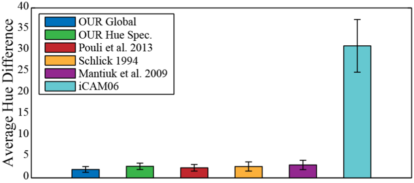
Figure 14: Hue differences and standard error over 20 images for the two proposed methods as well as alternative techniques.

IV-B Phsychopysical Evaluation

Typically, when compressing the gamut of an image for a particular display, the goal is to preserve the color appearance and general quality of the image as much as possible, while conforming to a more limited gamut. To assess the ability of our method to preserve image quality despite gamut restrictions, we have performed a psychophysical study. We used a two-alternative forced choice design, with the linearly scaled HDR reference shown at the same time, allowing us to assess the fidelity of the color reproduction of the processed images compared to the HDR input.

There were 13 participants (8 males and 5 females) in this experiment, who were between 22 and 25 years old, and all had normal or corrected-to-normal vision as well as normal color vision. Based on a pilot study comparing our chroma compression method against the iCAM06 model [6], the SCACLIP gamut compression method [9], and the correction methods of Mantiuk et al. [4] and Pouli et al. [5], we opted for comparing our method against the method of Mantiuk et al. [4] and the method of Pouli et al. [5] in a complete experiment, as the remaining methods were significantly less preferred. We also included the uncorrected tone mapped image in our evaluation which serves as our baseline result.

In our evaluation, the 13 participants viewed the differently processed results for 6 different scenes in pairwise comparisons between the alternative methods and were asked to select in each case the image that has the reproduction of color closest to the HDR image, which was shown as linearly scaled on the same screen. A colorimetric calibrated NEC MultiSync P241W sRGB monitor was used for this experiment. As it is not possible to accurately reproduce the HDR ground truth on this monitor, users could control the exposure for the HDR image manually, allowing them to more accurately compare the processed results with the ground truth image.

Detailed results are shown in Figure 15. We performed significance analysis on the experiment results computing the $\chi^{2}$ value and agreement coefficient. Overall, the $\chi^{2}$ value was 21.23 with an agreement coefficient of 0.033. At a 0.05% significance level, the critical $\chi^{2}$ value is 12.59, indicating that our results are significant. We note however that the agreement between participants was not very high. By further analyzing our results for individual images, we observed that participants agreed in their choices for some images, while agreement was lower for other images. We also observed that images with higher agreement were generally more saturated and colorful. Based on that, we repeated our analysis, but splitting the images into two groups depending on overall saturation: for the saturated group, $\chi^{2}=53.38$ (agreement coeff. 0.315) while for the less saturated group, $\chi^{2}=6.69$ (agreement coeff. 0.002). These results suggest that the benefit of our method is more visible in more colorful images with higher saturation, which is to be expected since these images are more likely to have out-of-gamut pixels.

Overall, we found that although the method of Mantiuk et al. [4] was chosen significantly fewer times, all other alternatives (our method, method of Pouli et al. [5] and uncorrected tone mapped only) were not found to be significantly different, suggesting that our method was found similarly visually pleasing by our participants as the uncorrected tonemapped results, while allowing for a controlled management of the gamut. As mapping out-of-gamut pixels inside the available gamut always presents a trade-off in visual quality, our method could be expected to offer a somewhat lower visual quality compared with the method of Pouli et al. [5]. However, our results show this not to be the case. The advantage of the present method relative to [5] is therefore the inclusion of unobtrusive gamut management.

Given that both the image and the display color space in this case was sRGB, gamut management was only necessary due to potential out-of-gamut issues introduced by the tone mapping process. The necessity for accurate gamut management, however, is likely to increase in the near future given the current consumer display trends towards higher dynamic range and wider gamut. The recent standard behind Ultra HD in particular (ITU-R Rec. BT.2020 [14]), specifies a considerably larger gamut than the previous widely adopted ITU-R Rec. BT.709 [15] color gamut, while concurrent proposals are pushing towards defining content at 4000 or even 10000 nits of peak luminance. At the same time, no displays exist that can achieve a full ITU-R Rec. BT.2020 gamut or these luminance levels. Consequently, both tone mapping and gamut management will be necessary to ensure that content is displayed as intended.

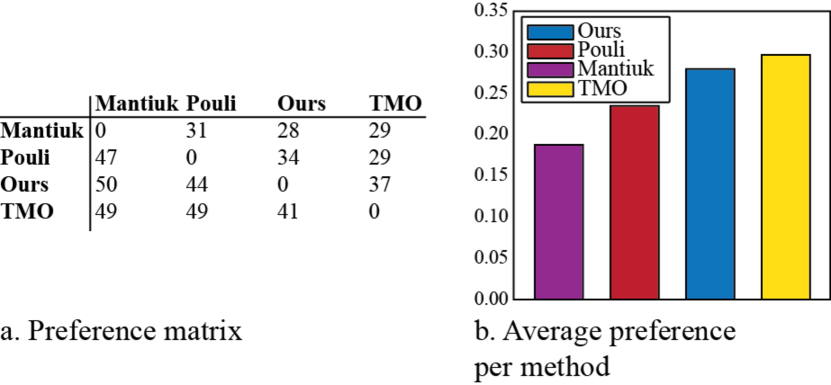
Figure 15: (a) Aggregated preference results from our experiment for the different tested methods. Each matrix cell represents the number of times the method in each row was chosen over the method in each column. (b) Average total preference per method.

V Conclusions

Typically tone mapping compresses the luminance range of images, while chromatic information is left untouched or is manually corrected as a post process. On the other hand, gamut mapping algorithms deal with both luminance and chromatic information and aim to map images from one gamut to another, but typically deal with small changes, mostly along the chromatic dimensions. In this paper, we show how gamut mapping techniques can be extended to the HDR domain, when the transitions between the input and output gamuts are often very large. We integrate tone mapping, chroma compression, and gamut management into a single framework that preserves the appearance of the HDR input, while preventing unwanted shifts and ensuring that the output image fits within the target gamut boundaries.

Within our proposed framework, we describe two chroma compression methods, each best suited for a different part of the imaging pipeline. We have evaluated our framework using several tone mapping operators and compared its results with traditional tone and gamut mapping techniques as well as a color correction formula to show the ability of our approach to overcome their drawbacks. We also showed that existing tone mapping operators can be naturally integrated into our framework, which enables the users to choose different operators for different applications.

VI Acknowledgments

This work was partially supported by Ministry of Science and Innovation Subprogramme Ramon y Cajal RYC-2011-09372, TIN2013-47276-C6-1-R from Spanish government, 2014 SGR 1232 from Catalan government and EC ”PARTHENOS” (GA no. 654119) from the Italian government.

References

- [1] E. Reinhard, G. Ward, S. Pattanaik, and P. Debevec, High Dynamic Range Imaging: Acquisition, Display and Image-Based Lighting, 2nd ed. San Francisco: Morgan Kaufmann, 2010.
- [2] F. Banterle, A. Artusi, K. Debattista, and A. Chalmers, Advanced High Dynamic Range Imaging: Theory and Practice. CRC Press, (AK Peters Ltd), 2011.
- [3] C. Schlick, “Quantization techniques for visualization of high dynamic range pictures,” Proceeding of the Fifth Eurographics Workshop on Rendering, pp. 7–18, 1994.
- [4] R. Mantiuk, R. Mantiuk, A. Tomaszweska, and W. Heidrich, “Color correction for tone mapping,” Computer Graphics Forum Journal, vol. 28, no. 2, 2009.
- [5] T. Pouli, A. Artusi, F. Banterle, A. O. Akyüz, H.-P. Seidel, and E. Reinhard, “Automatic saturation correction for dynamic range management algorithms,” in Color Imaging Conference, 2013.
- [6] J. Kuang, G. M. Johnson, and M. D. Fairchild, “iCAM06: A refined image appearance model for hdr image rendering,” Journal of Visual Communication and Image Representation, vol. 18, no. 5, pp. 406 – 414, 2007. [Online]. Available: http://www.sciencedirect.com/science/article/pii/S1047320307000533
- [7] E. Reinhard, T. Pouli, T. Kunkel, B. Long, A. Ballestad, and G. Damberg, “Calibrated image appearance reproduction,” ACM Transactions on Graphics, vol. 31, no. 6, p. 201, 2012.
- [8] E. Reinhard, M. Stark, P. Shirley, and J. Ferwerda, “Photographic tone reproduction for digital images,” ACM Transactions on Graphics, vol. 21, no. 3, pp. 267–276, 2002.
- [9] N. Bonnier, F. Schmitt, M. Hull, and C. Leynadier, “Spatial and color adaptive gamut mapping: A mathematical framework and two new algorithms,” Proc. of the 15th Color Imaging Conference, pp. 267–272, 2007.
- [10] J. Morovic, Color Gamut Mapping, 1st ed. The Wiley-IS&T Series in Imaging Science and Technology, 2008.
- [11] F. Drago, K. Myszkowski, T. Annen, and N. Chiba, “Adaptive logarithmic mapping for displaying high contrast scenes,” Computer Graphics Forum, vol. 22, no. 3, 2003.
- [12] M. Ashikhmin, “A tone mapping algorithm for high contrast images,” in Proceedings of the 13th Eurographics workshop on Rendering, ser. EGRW ’02. Aire-la-Ville, Switzerland, Switzerland: Eurographics Association, 2002, pp. 145–156. [Online]. Available: http://dl.acm.org/citation.cfm?id=581896.581916
- [13] S. Shen, “Color difference formula and uniform color space modeling and evaluation,” Ph.D. dissertation, Rochester Institute of Technology, 2009.
- [14] ITU, “Recommendation ITU-R BT.2020: Parameter values for ultra-high definition television systems for production and international programme exchange,” International Telecommunications Union, 2012.
- [15] ——, “Recommendation ITU-R BT.709-3: Parameter values for the HDTV standards for production and international programme exchange,” International Telecommunications Union, 1998.