Quantum mechanical treatment of large spin baths

Abstract

The electronic spin in quantum dots can be described by central spin models (CSMs) with a very large number $N_{\text{eff}}\approx 10^{4}$ to $10^{6}$ of bath spins posing a tremendous challenge to theoretical simulations. Here, a fully quantum mechanical theory is developed for the limit $N_{\text{eff}}\to\infty$ by means of iterated equations of motion (iEoM). We find that the CSM can be mapped to a four-dimensional impurity coupled to a non-interacting bosonic bath in this limit. Remarkably, even for infinite bath the CSM does not become completely classical. The data obtained by the proposed iEoM approach is tested successfully against data from other, established approaches. Thus, the iEoM mapping extends the set of theoretical tools which can be used to understand the spin dynamics in large CSMs.

I Introduction

Since the proposal to use the electronic spin of excess electrons or holes in quantum dots Loss and DiVincenzo (1998) for the realization of quantum bits Nielsen and Chuang (2000) an enormous research activity has started, both experimentally Hanson et al. (2007); Urbaszek et al. (2013); Warburton (2013); Chekhovich et al. (2013) and theoretically Merkulov et al. (2002); Schliemann et al. (2003); Coish and Baugh (2009); Fischer and Loss (2009); Ribeiro and Burkard (2013). From the theoretical side, the isotropic central spin model (CSM), first introduced by Gaudin for its integrability Gaudin (1976, 1983), has become the canonical starting point although various additional couplings matter as well such as the dipole-dipole interaction between the nuclear spins forming the spin bath Merkulov et al. (2002); Schliemann et al. (2003), spin anisotropies Fischer et al. (2008); Testelin et al. (2009); Hackmann and Anders (2014) including spin-orbit couplings Nowack et al. (2007); Rančić and Burkard (2014), and the quadrupolar couplings of the bath spins Chekhovich et al. (2012); Sinitsyn et al. (2012); Hackmann et al. (2015). In the present work, we restrict ourselves to the isotropic CSM without further couplings.

In self-assembled quantum dots, $N_{\text{eff}}\approx 10^{5}$ bath spins are relevant Merkulov et al. (2002); Schliemann et al. (2003); Lee et al. (2005); Petrov et al. (2008) or even $N_{\text{eff}}\approx 10^{6}$ in electrostatically confined quantum dots Petta et al. (2005). This enormous number makes the reliable computation of the central spin dynamics extremely challenging despite the integrability of the model Faribault and Schuricht (2013a, b). Only a few tens of spins can be treated exactly and this remains true for most numerical approaches as well such as exact diagonalization Schliemann et al. (2003); Cywiński et al. (2010), Chebyshev expansion (CE) Dobrovitski et al. (2003); Dobrovitski and De Raedt (2003); Hackmann and Anders (2014), or a direct evolution of the density matrices via the Liouvillean Beugeling et al. (2016). Density-matrix renormalization group (DMRG) can cope with up to about 1000 spins, but it is restricted to short times Stanek et al. (2013, 2014); Gravert et al. (2016). Persisting correlations at infinite times can be dealt with by mathematically rigorous bounds Uhrig et al. (2014); Seifert et al. (2016). Techniques based on rate equations or on non-Markovian master equations give access to large bath sizes, but they are well justified only for sufficiently strong external fields Khaetskii et al. (2002, 2003); Coish and Loss (2004); Breuer et al. (2004); Fischer and Breuer (2007); Ferraro et al. (2008); Coish et al. (2010); Barnes et al. (2012); Rudner and Levitov (2007). So far, the same holds true for an approach based on equations of motion Deng and Hu (2006, 2008). Finally, cluster expansion techniques are powerful, but restricted by the maximum treatable cluster size. This restriction implies a time threshold up to which the results are reliable Witzel et al. (2005); Witzel and Das Sarma (2006); Maze et al. (2008); Yang and Liu (2008, 2009); Witzel et al. (2012).

The classical counterpart of the CSM approximates the quantum mechanical spin dynamics well Chen et al. (2007); Stanek et al. (2014), see also the related approach based on time-dependent mean-fields Al-Hassanieh et al. (2006); Zhang et al. (2006). This behavior can be justified either by the saddle point approximation for a large spin bath Chen et al. (2007) or even simpler by the quantum fluctuations of the Overhauser field which are suppressed by the limit of infinite spin bath Stanek et al. (2013). Until recently, however, even the classical CSM could not be treated for bath sizes comparable to the experimental ones. The Lanczos approach or the exponential discretization of the spectral density has provided a breakthrough to simulate infinitely large systems up to very large times Fauseweh et al. (2017). Classical or semiclassical simulations capture many experimental observations nicely Hackmann et al. (2014); Jäschke et al. (2017).

Yet, the quantum mechanical dynamics is not fully captured by the classical simulation. While the argument for classical properties of the Overhauser field is strong, there is no such argument for the central spin $S=1/2$. Thus, there still remains the open issue to identify specific quantum mechanical effects and to describe them quantitatively. The measurement of four-point correlations provides experimental access to quantities which depend strongly on the sequence of operators acting on the central spin and hence on its quantumness Press et al. (2010); Bechtold et al. (2016); Fröhling and Anders (2017).

For these reasons, the present paper proposes an approach to the quantum mechanical CSM valid for large spin baths. It is based on the equations of motion for spin operators Uhrig (2009); Kalthoff et al. (2017) and an expansion in the inverse effective number of bath spins $1/N_{\text{eff}}$.

The key finding of our approach is that the isotropic CSM can be mapped to a four-dimensional impurity coupled to a non-interacting bosonic bath. This mapping provides an alternative view on the CSM in the limit of a large bath. In order to establish this mapping, we exploit the simplifying limit of large spin baths to compute quantum mechanical traces of sums of large numbers of spins Seifert et al. (2016). In this way, we evaluate the central spin autocorrelation function with and without a magnetic field. In the limit $N_{\text{eff}}\to\infty$, the traces reduce to Gaussian integrals. The approach is benchmarked against data from exact methods, available only for small number of bath spins. Even though this is not the optimum regime for the application of the developped approach, the agreement found is promising.

The setup of the paper is the following. After this introduction we introduce the model in Sect. II and derive the advocated approach in Sect. III. Then, we show in Sect. IV how its results compare with data obtained by established techniques in order to underline the validity of its derivation. Finally, the results are summarized and an outlook is given in Sect. V.

II Model

In the present article, we focus on the paradigmatic isotropic central spin model comprising a central spin $\vec{S}_{0}$ with $S=1/2$ and bath spins $\vec{S}_{i}$ with $S=1/2$

$$\mathcal{H}=\vec{S}_{0}\cdot\sum\limits_{i=1}^{N}J_{i}\vec{S}_{i},$$ (1)

where the $J_{i}$ are the hyperfine couplings. The field $\vec{B}$ composed of all bath spins

$$\vec{B}=\sum\limits_{i=1}^{N}J_{i}\vec{S}_{i}$$ (2)

is called the Overhauser field. For concreteness, we will consider the following generic set of hyperfine couplings

$$J_{i}=C\exp(-i\gamma),\quad i\in\mathbb{N},$$ (3)

which decrease exponentially as function of the parameter $\gamma$. This is the typical scenario encountered in electronic quantum dots where the coupling is proportional to the probability of the electronic wave function at the location of the nuclear spin Merkulov et al. (2002); Schliemann et al. (2003). In two dimensions, the above parametrization results from Gaussian wave functions Fauseweh et al. (2017) and has been used in many previous studies as well Coish and Loss (2004); Faribault and Schuricht (2013a, b); Seifert et al. (2016). Note that (3) describes the couplings for a single CSM. If we want to describe an ensemble of quantum dots, the results have to be averaged over the distribution of the different couplings for different quantum dots.

In real quantum dots, further interactions such as dipole-dipole and quadrupolar couplings of the nuclear spins play a role on very long time scales. Here we restrict ourselves to the isotropic CSM (1) for simplicity to establish our new approach which solves this model in the physically relevant limit of an infinite spin bath.

We emphasize that we can treat an infinitely large spin bath because $i$ is not limited, i.e., the total number of bath spins $N$ may be set to infinity. But the physically relevant number is the finite effective number of bath spins $N_{\text{eff}}$, i.e., the number of bath spins which are substantially coupled. This number can be defined via the ratio of the squared sum of all couplings and the sum of all squared couplings Merkulov et al. (2002); Schliemann et al. (2003); Stanek et al. (2013, 2014); Fauseweh et al. (2017). The latter is given by

$$J_{\text{Q}}^{2}=\sum\limits_{i=1}^{N}J_{i}^{2}.$$ (4)

Note that $J_{\text{Q}}$ sets the energy scale of the dynamics on short time scales, i.e., it is set to unity in the numerical evaluations below. The effective number $N_{\text{eff}}$ of bath spins reads Fauseweh et al. (2017)

$$N_{\text{eff}}=2/\gamma+O(\gamma).$$ (5)

Thus, $\gamma\approx 10^{-5}$ to $10^{-6}$ is an excellent small parameter suitable to control a perturbative approach systematically. We stress that the normalization $J_{\text{Q}}=1$ also implies that the overall prefactor $C$ in (3) is given by $\sqrt{2\gamma}$ in the limit of small $\gamma$, i.e., it scales like $1/\sqrt{N_{\text{eff}}}$. This means that the contribution of each individual bath spin alone is negligible. Only suitable sums over all of them will have an impact which is relevant in the limit $N_{\text{eff}}\to\infty$.

III Derivation of the approach

III.1 General equation of motion of operators

We are interested in the dynamical spin-spin correlation function of the CSM. Thus we start from the Heisenberg equation of motion for an arbitrary operator $A$

$$\partial_{t}A=i[\mathcal{H},A]=i\mathcal{L}A,$$ (6)

where we introduced the Liouville operator $\mathcal{L}$ which acts as linear mapping on the vector space of operators. To make the vector space of operators a Hilbert space we introduce the scalar product of Frobenius type

$$\left\langle\left\langle A|B\right\rangle\right\rangle:=\frac{1}{d}\text{Tr}(A^{\dagger}B),$$ (7)

where $d$ is the dimension of the Hilbert space of states. Clearly, this definition requires that the local Hilbert space is finite so that this definition only works for spins or fermions on discrete sites Kalthoff et al. (2017). Then it corresponds to the expectation values of the two operators in the limit of infinite temperature where the system is completely disordered so that any state is equally probable.

Bosonic degrees of freedom can only be treated at the price of a truncation of their local Hilbert spaces. Note, however, that the above definition works also for models with an infinite number of sites as long as the operators $A$ and $B$ affect only a finite number of sites, i.e., they act on finite subclusters. This is the situation we are dealing with here.

The key advantage of the definition (7) in comparison to other choices is that the Liouville operator $\mathcal{L}$ is self-adjoint with respect to this scalar product Kalthoff et al. (2017)

$$\left\langle\left\langle A|\mathcal{L}B\right\rangle\right\rangle=\left\langle\left\langle\mathcal{L}A|B\right\rangle\right\rangle.$$ (8)

Hence, the operator dynamics induced by $\mathcal{L}$ shows oscillatory behavior or, possibly complicated, superpositions of oscillations. But no power law or exponential divergences occur, even if truncated orthonormal operator bases are used. We emphasize that superpositions of oscillations are precisely what one expects for quantum mechanical models.

The application of the equation of motion to the CSM suggests to consider an operator basis made from products of components of spin operators at different sites Kalthoff et al. (2017). In principle, this does work and we implemented it (not shown). But we quickly realized that one has to track essentially all possible combinations of operators on all sites in order to obtain reliable results. Hence, the direct application of the equations of motion quickly becomes impractical.

This conclusion is corroborated by an analytical argument. Suppose for simplicity that the bath spins do not move. Then the Overhauser field $\vec{B}=B\vec{n}$ is a static magnetic field of size $B$ pointing in the direction given by the unit vector $\vec{n}$ about which the central spin $\vec{S}_{0}$ precesses according to Merkulov et al. (2002)

$$\vec{S}_{0}(t) =\vec{n}(\vec{n}\cdot\vec{S}_{0}(0))+[\vec{S}_{0}(0)-(\vec{n}\cdot\vec{S}_{0}(0))\vec{n}]\cos(Bt)$$

$$-\{\vec{S}_{0}(0)\times\vec{n}\}\sin(Bt).$$ (9)

Note that the sign in the last term has been corrected. This equation has been used by Merkulov et al. in order to describe the spin dynamics in quantum dots by averaging it over a Gaussian distribution of the Overhauser field Merkulov et al. (2002).

Expression (III.1) reveals that arbitrary high powers of the modulus $B$ of the Overhauser field $\vec{B}$ are required in order to capture the dynamics for long times. Since the Overhauser field is the weighted sum over all bath spin operators it is implied that products with arbitrarily many factors of spin operators are important. We will come back to this point later. The second message of the result (III.1) is that it is not the individual bath spin which influences the central spin, but sums of them.

III.2 Generalized Overhauser fields

The time evolution of the central spin is governed by the couplings to the spin bath. However, as we see from Eq. (3) and the subsequent normalization implying that the prefactor $C\propto\sqrt{\gamma}$ the individual coupling $J_{i}$ scales like $\mathcal{O}(1/\sqrt{N_{\text{eff}}})$, making it almost negligibly small for a realistic number of bath spins. Hence, the dynamics of the individual bath spin is not a promising starting point in the limit $N_{\text{eff}}\rightarrow\infty$. We conclude that it is not the single coupling which is important, but rather weighted sums of all couplings.

The first and most important sum is the Overhauser field $\vec{B}$ itself, including all couplings in linear order. This was first realized in Ref. Merkulov et al., 2002. However, if we want to describe the time evolution exactly, higher orders of the individual couplings need to be taken into account. Using the same argument as before, the non-linear contributions of the individual couplings $J_{i}$ vanish in the limit $N_{\text{eff}}\rightarrow\infty$. But extensive sums of the non-linear contributions remain finite. This observation was first used in the efficient description of the dynamics of the classical CSM Fauseweh et al. (2017), but also carries over to the quantum mechanical case as we show in the following.

We adopt the idea of introducing generalized Overhauser fields where the weight of each spin is given by polynomials $p_{j}$ of the couplings $J_{i}$

$$\vec{P}_{j}:=2\sum_{i=1}^{N}p_{j}(J_{i})\vec{S}_{i},\quad j\in\mathbb{N}.$$ (10)

Note that $p_{j}(x)$ are polynomials of degree $j$. This definition deviates from the classical one by a factor of 2 in order to ensure orthonormalization, see below. First, we require that the polynomials are orthonormal with respect to the following scalar product for real functions

$$\left(p_{j}|p_{k}\right) :=\sum_{i=1}^{N}p_{j}(J_{i})p_{k}(J_{i})$$ (11a)

$$=\delta_{jk}.$$ (11b)

Thus, the theory of orthogonal polynomials tells us that they can be reconstructed iteratively following the standard Lanczos procedure

$$xp_{j}(x)=\beta_{j}p_{j+1}(x)+\alpha_{j}p_{j}(x)+\beta_{j-1}p_{j-1}(x)$$ (12)

where $p_{0}(x)=0$, $p_{1}(x)=x$ so that $\vec{P}_{1}:=2\vec{B}$ is the usual Overhauser field up to a factor of 2. The recursion coefficients $\alpha_{j}$ and $\beta_{j}$ result from

$$\beta_{j-1} =\left(x{p}_{j}|p_{j-1}\right)$$ (13a)

$$\alpha_{j} :=\left(x{p}_{j}|p_{j}\right)$$ (13b)

$$\beta_{j} :=\sqrt{\left|x{p}_{j}-\alpha_{j}p_{j}-\beta_{j-1}p_{j-1}\right|^{2}}.$$ (13c)

For the exponential couplings in Eq. (3), these coefficients are explicitly derived in Ref. Fauseweh et al., 2017 for $\gamma\ll 1$. They read

$$\alpha_{j} =\frac{4j^{2}}{4j^{2}-1}\sqrt{\frac{\gamma}{2}}$$ (14a)

$$\beta_{j} =\frac{\sqrt{j(j+1)}}{2j+1}\sqrt{\frac{\gamma}{2}}.$$ (14b)

We use these recursion coefficients to illustrate the first three generalized Overhauser fields

$$\vec{P}_{1} =2\sqrt{\gamma}\sum_{i=1}^{N}\overline{J}_{i}\vec{S}_{i}$$ (15a)

$$\vec{P}_{2} =2\sqrt{\gamma}\sum_{i=1}^{N}(3\overline{J}_{i}-\sqrt{8})\overline{J}_{i}\vec{S}_{i}$$ (15b)

$$\vec{P}_{3} =2\sqrt{\gamma}\sum_{i=1}^{N}\sqrt{3}(5\overline{J}^{2}_{i}-6\sqrt{2}\overline{J}_{i}+3)\overline{J}_{i}\vec{S}_{i},$$ (15c)

where $\overline{J}_{i}:=J_{i}/\sqrt{\gamma}$.

Using the notation of the generalized Overhauser fields the Hamiltonian can be denoted

$$\mathcal{H}=\frac{1}{2}\vec{S}_{0}\cdot\vec{P}_{1}.$$ (16)

For later use we draw the reader’s attention to the fact that the coefficients $\alpha_{j}$ and $\beta_{j}$ are of order $\sqrt{\gamma}$, see (14) and the comprehensive discussion in Ref. Fauseweh et al., 2017.

It is known Pettifor and Weaire (1985); Viswanath and Müller (1994) that the recursion coefficients can be understood as the matrix elements of the real symmetric tridiagonal matrix

$$\mathbold{T}=\begin{pmatrix}\alpha_{1}&\beta_{1}&0&0&\dots\\ \beta_{1}&\alpha_{2}&\beta_{2}&0&\dots\\ 0&\beta_{2}&\alpha_{3}&\beta_{3}&\dots\\ \vdots&\vdots&\ddots&\ddots&\ddots\end{pmatrix}$$ (17)

which acts on the vector of orthonormal polynomials

$$\mathbold{p}(x)=\left(p_{1}(x),\,p_{2}(x),\,...\,p_{n}(x)\right)^{T}$$ (18)

according to

$$x\mathbold{p}(x)=\mathbold{T}\mathbold{p}(x).$$ (19)

This representation is useful because it tells us how to truncate. Truncating the matrix dimension of $\mathbold{T}$ to the positive integer $N_{\text{tr}}$ we introduce an effective truncation scheme for the recursion coefficients. We keep those which lie within the $N_{\text{tr}}\times N_{\text{tr}}$ dimensional upper left submatrix of $\mathbold{T}$. This has proven to be a powerful approach in the classical calculations Fauseweh et al. (2017).

We point out that due to the construction from orthogonal polynomials, the generalized Overhauser fields are orthonormal with respect to the Frobenius norm

$$\left\langle\left\langle P^{\alpha}_{j}|P^{\beta}_{k}\right\rangle\right\rangle=\delta_{\alpha\beta}\delta_{jk}.$$ (20)

This is explicitly derived in Appendix A.

III.3 Higher powers of the generalized Overhauser fields

In the definition of the generalized Overhauser fields $\vec{P}_{j}$ we introduced higher powers of the couplings $J_{i}$ by means of certain orthogonal polynomials. The generalized Overhauser fields are the above mentioned suitably weighted sums over the spin operators. The weights are given by the orthogonal polynomials. The precise form of these polynomials depends on the set of couplings. However, each generalized Overhauser field is still linear in the spin operators, see Eq. (10). In case of commuting classical vectors this was sufficient Fauseweh et al. (2017).

For the quantum mechanical dynamics we are studying here we need more, namely higher powers of the generalized Overhauser fields $P^{\alpha}_{j}$. We show here that the appropriate way to consider higher powers of the Overhauser fields is to consider Hermite polynomials $H_{n}$ of them. We emphasize that Hermite polynomials are again orthogonal polynomials, but they used here for something different than the $p_{j}$: the $p_{j}$ are polynomials in the couplings while the Hermite polynomials to be introduced are polynomials in the generalized Overhauser fields.

In order to motivate that we need higher powers of the Overhauser fields let us consider $A=S_{0}^{z}$ and insert it into the right hand side of the equation of motion (6) yielding $i[H,S_{0}^{z}]=(S_{0}^{y}P_{1}^{x}-S_{0}^{x}P_{1}^{y})/2$. This expression is linear in the Overhauser field. But if we iterate it as we have to do to capture the quadratic time dependence, we consider $A=S_{0}^{y}P_{1}^{x}-S_{0}^{x}P_{1}^{y}$. A simple calculation reveals that $[H,A]$ comprises terms such as $(P_{1}^{x})^{2}$, $P_{1}^{x}P_{1}^{z}$, $(P_{1}^{y})^{2}$, or $P_{1}^{y}P_{1}^{z}$, i.e., quadratic powers of the Overhauser fields occur. This is just meant as simple motivating example. In computing the long-time dynamics arbitrarily high powers will arise.

Therefore, we include such higher powers in the operator basis and thus have to consider their norm and scalar products with other terms in the operator basis. Hence, we are facing the evaluation of traces of the general type

$$I=\text{Tr}\left(P_{j_{1}}^{\alpha_{1}}P_{j_{2}}^{\alpha_{2}}P_{j_{3}}^{\alpha_{3}}\ldots P_{j_{n-1}}^{\alpha_{n-1}}P_{j_{n}}^{\alpha_{n}}\right)$$ (21)

where the trace refers to the Hilbert space of the bath spins. The fundamental observation starts from the normalization $\left\langle\left\langle P^{\alpha}_{j}|P^{\alpha}_{j}\right\rangle\right\rangle=1$ which results from a weighted sum over the trace of $(S_{i}^{\alpha})^{2}=1/4$. Since $N_{\text{eff}}$ spins are substantially coupled each single spin of them contributes only $O(1/N_{\text{eff}})$. Hence, the prefactor $p_{j}(J_{i})$ of $S_{i}^{\alpha}$ in $P^{\alpha}_{j}$ is of order $1/\sqrt{N_{\text{eff}}}$, see also Eq. (14).

For $I$ to take a non-zero value even in the limit $N_{\text{eff}}\to\infty$ one has to combine the operators $P_{j_{m}}^{\alpha_{m}}$ to pairs. Let us call one choice of combining all $P_{j_{m}}^{\alpha_{m}}$ to pairs a ‘pairing’. In each pair, the sum over the individual bath spins runs over $N_{\text{eff}}$ sites and each summand contributes in order $4/N_{\text{eff}}$ so that the pair yields a non-vanishing contribution. So, the product of all pairs in each pairing yields a finite contribution in the limit $N_{\text{eff}}\to\infty$. The total value of $I$ results from all possible pairings.

Let us consider triples (generally $n$-tuples with $n>2$) of the $P_{j_{m}}^{\alpha_{m}}$ instead of pairs. By this we mean, that the summation over the bath spins $S_{i}^{\alpha}$ is done over trilinear terms such as $S_{i}^{x}S_{i}^{y}S_{i}^{z}$ where each factor is taken from one generalized Overhauser field in the triple. Then the summation is more restricted so that in total less summations can be done. This reduces the contribution by at least a factor $1/N_{\text{eff}}$. For instance, the trace

$$X:=\frac{1}{d}\text{Tr}\left(P_{1}^{x}P_{2}^{y}P_{2}^{z}P_{1}^{x}P_{2}^{y}P_{2}^{z}\right)$$ (22)

splits into a product of three pairs

$$X_{\text{pair}} =\left(\sum_{i=1}^{N}p_{1}^{2}(J_{i})\text{Tr}(S^{x}_{i})^{2}\right)\left(\sum_{i=1}^{N}p_{2}^{2}(J_{i})\text{Tr}(S^{y}_{i})^{2}\right)$$

$$\qquad\cdot\left(\sum_{i=1}^{N}p_{2}^{2}(J_{i})\text{Tr}(S^{z}_{i})^{2}\right)$$ (23)

and into a product of two triples

$$X_{\text{triple}}=K\left(\sum_{i=1}^{N}p_{1}(J_{i})p_{2}^{2}(J_{i})\text{Tr}(S^{x}_{i}S^{y}_{i}S^{z}_{i})\right)^{2}$$ (24)

with some combinatorial factor $K$ and similar products of a quadruple and a pair and a single 6-tuple. Note that the trace in (22) refers to the Hilbert space of the total system while the traces in (III.3) and (24) refer to the local Hilbert space of a single bath spin $\vec{S}_{i}$. The crucial observation is that $X_{\text{pair}}$ is precisely unity due to the orthonomalization of the polynomials $p_{j}$ while $X_{\text{triple}}$ is of order $1/N_{\text{eff}}$, i.e., subleading, because there is one summation less. The same holds for any combinations of $n$-tuples with $n>2$ so that only pairings need to be considered in leading order. In particular, we learn that $n$ has to be even. Due to the orthonormalization each pair $P^{\alpha}_{j},P^{\beta}_{k}$ yields the factor $\left\langle\left\langle P^{\alpha}_{j}|P^{\beta}_{k}\right\rangle\right\rangle=\delta_{\alpha\beta}\delta_{jk}$, cf. Eq. (20).

We conclude that the computation of the leading term of $I$ in an expansion in $1/N_{\text{eff}}$ is straightforward. It can be simplified even further by observing that the computation of all pairings is exactly what is done in the evaluation of expectation values of random variables fulfilling Gaussian distributions. This is the content of Wick’s theorem for classical fields Wegner (2000).

We arrive at the stunning conclusion that the computation of the leading order of the quantum mechanical traces $I$ amounts to the calculation of classical expectation values of the Gaussian random variables $P^{\alpha}_{j}$ with the correlations given by the scalar product (60). This was first observed in Ref. Seifert et al., 2016. Corrections are of order $1/N_{\text{eff}}$.

We emphasize the important implication that the sequence of the operators in the trace in (21) does not matter. This is obviously true for the classical calculations. It does not represent a contradiction to the quantum mechanical nature of the spins in the bath because it only holds for the leading contribution in an expansion in $1/N_{\text{eff}}$. In Appendix B, we verify explicitly that the non-vanishing commutators are less relevant with respect to an expansion in $1/N_{\text{eff}}$.

We summarize that the computation of the Frobenius scalar product for functions of the generalized Overhauser field is tantamount to computing these functions with respect to Gaussian weights. But we emphasize that we are developing a fully quantum mechanical treatment although the traces are computed via classical integrals. These classical Gaussian integrals are identical to the quantum mechanical traces up to corrections of the order of $1/N_{\text{eff}}\approx 10^{-5}$ or even smaller.

In view of the Gaussian weights it suggests itself to consider Hermite polynomials to describe general functions of the Overhauser fields because they are the orthogonal polynomials for a Gaussian weight function Abramowitz and Stegun (1964); Bronstein et al. (2008). We define the normalized Hermite polynomials

$$H_{n}(x)=\frac{1}{\sqrt{n!}}(-1)^{n}e^{\frac{x^{2}}{2}}\frac{d^{n}}{dx^{n}}e^{-\frac{x^{2}}{2}}$$ (25)

where the factor $1/\sqrt{n!}$ is added for notational convenience, see below, beyond the standard definition in mathematical text books. As pointed out above, these Hermite polynomials are orthonormalized with respect to a Gaussian weight function $w(x)=(\sqrt{2\pi})^{-1}\exp(-x^{2}/2)$, i.e., they fulfil

$$\frac{1}{\sqrt{2\pi}}\int_{-\infty}^{\infty}H_{n}(x)H_{m}(x)e^{-\frac{x^{2}}{2}}dx=\delta_{nm}.$$ (26)

Furthermore, the relations

$$xH_{n}(x) =\sqrt{n}H_{n-1}(x)+\sqrt{n+1}H_{n+1}(x)\quad,$$ (27a)

$$\frac{d}{dx}H_{n}(x) =\sqrt{n}H_{n-1}(x)$$ (27b)

hold and are very well known to physicists because they are the eigen functions of the harmonic oscillators. We will exploit the analogy to harmonic oscillators further below.

The Hermite polynomials provide a transparent way to include higher powers of the generalized Overhauser fields because in leading order in $1/N_{\text{eff}}$ we have

$$\left\langle\left\langle H_{n}({P}_{j}^{\alpha})\left|H_{m}({P}_{j}^{\alpha})\right.\right\rangle\right\rangle=$$

$$\quad=\frac{1}{d}\text{Tr}\left(\left(H_{n}({P}_{j}^{\alpha})\right)^{\dagger}H_{m}({P}_{j}^{\alpha})\right)$$ (28a)

$$\quad=\frac{1}{\sqrt{2\pi}}\int_{-\infty}^{\infty}H_{n}(P_{j}^{\alpha})H_{m}(P_{j}^{\alpha})e^{-\frac{1}{2}\left(P_{j}^{\alpha}\right)^{2}}dP_{j}^{\alpha}$$ (28b)

$$\quad=\delta_{mn}$$ (28c)

where $d$ stands for the dimension of the underlying Hilbert space of bath spins.

Next, we define operators which will form the basis in the Hilbert space of operators. As usual, the operators acting on the central spin are described by Pauli matrices ${\sigma}_{m}$ with $m\in\{0,1,2,3\}$ where $\sigma_{0}$ is the identity matrix. Furthermore, we have to describe powers of the generalized Overhauser fields to describe the dynamics of the spin bath. As explained above, Hermite polynomials with the generalized Overhauser fields as arguments are the appropriate choice because they imply orthonormality of the operator basis. Concretely, we use the shorthand

$${H_{n_{j,\alpha}}:=H_{n_{j,\alpha}}({P}_{j}^{\alpha})},$$ (29)

where $n_{j,\alpha}$ carries its two subscripts because the degree of the Hermite polynomial depends on the index of the Overhauser field and its component $\alpha\in\{x,y,z\}$. Then, a general basis operator reads

$$\hat{b}^{m}_{\mathbold{n}} :={\sigma}_{m}A_{\mathbold{n}}$$ (30a)

$$A_{\mathbold{n}} :=H_{n_{1,x}}H_{n_{1,y}}H_{n_{1,z}}H_{n_{2,x}}...$$ (30b)

$$\mathbold{n} :=(n_{1,x},\,n_{1,y},\,\ldots,\,n_{N_{\text{tr}},z}),$$ (30c)

where the $3N_{\text{tr}}$-tuple $\mathbold{n}$ as defined above stores the degrees of the respective Hermite polynomials. For the notation to be unique, the sequence of non-negative integers $n_{j,\alpha}$ is defined as shown in (30c). But for the evaluation of traces and hence of the Frobenius scalar products it does not matter in leading order in $1/N_{\text{eff}}$.

The orthonormality of the $\hat{b}_{m}^{\mathbold{n}}$ results from

$$\left\langle\left\langle\hat{b}^{k}_{\mathbold{n}}\left|\hat{b}^{l}_{\mathbold{m}}\right.\right\rangle\right\rangle=$$

$$\quad=\frac{1}{d}\text{Tr}\left(\prod_{j=1}^{N_{\text{tr}}}\prod_{\alpha}\left(\sigma_{k}H_{n_{j,\alpha}}\right)^{\dagger}\sigma_{l}H_{m_{j,\alpha}}\right)$$ (31a)

$$\quad=\frac{1}{2}\text{Tr}\left(\sigma_{k}\sigma_{l}\right)\frac{1}{{2^{N}}}\text{Tr}\left(\prod_{j=1}^{N_{\text{tr}}}\prod_{\alpha}H_{n_{j,\alpha}}H_{m_{j,\alpha}}\right)$$ (31b)

$$\quad=\delta_{kl}\delta_{\mathbold{n}\mathbold{m}},$$ (31c)

where we used again that the traces can be computed by Gaussian integrals and that the Hermite polynomials are orthonormal with respect to these integrals. The Kronecker symbol $\delta_{\mathbold{n}\mathbold{m}}$ is unity if both sequences of non-negative integers $\mathbold{n}$ and $\mathbold{m}$ are equal; otherwise it vanishes. Thus, the basis spanned by the operators $\hat{b}_{m}^{\mathbold{n}}$ provides an excellent starting point to treat the equations of motion of the CSM quantitatively.

III.4 Specific equation of motion

In this next step, we establish the equations of motion for the developed basis of operator. Hence, we have to know from where we start and how the Liouville operator acts on $\hat{b}^{m}_{\mathbold{n}}$.

We aim at the isotropic CSM without magnetic field in the first place. We intend to compute the $\langle S^{z}(t)S^{z}(0)\rangle$ correlation as function of time. Thus, the initial basis operator is the $z$-component of the central spin while all bath spins are supposed to be in a completely disordered state, i.e., there is no operator acting on any bath spin. This choice is indicated by the extremely small couplings $J_{i}$ which are exceeded by the thermal energy even at 10K so that the spin bath can be considered to be at infinite temperature Coish and Baugh (2009); Urbaszek et al. (2013). Thus, initially the spin bath is described by the Hermite polynomials $H_{0}$ equal to the identity for all $j$ and all $\alpha$, i.e., $H_{0}({P}_{j}^{\alpha})=\mathds{1}$. The starting operator is

$$\hat{b}^{3}_{\mathbold{o}}={\sigma}_{3}H_{0}H_{0}H_{0}....$$ (32)

In order to obtain the time evolution we have to compute the action of $\mathcal{L}$ on the basis operators which amounts to computing the commutator between the Hamiltonian $\mathcal{H}$ in (16) and $\hat{b}^{m}_{\mathbold{n}}$, which is a product of an operator $\sigma_{m}$ acting on the central spin and of the operator $A_{\mathbold}{n}$ acting on the spin bath. Similarly, the Hamiltonian consists of a sum of products of an operator acting on the central spin and an operator acting on the spin bath. If we use $C$ and $C^{\prime}$ for operators of the central spin and $A$ and $A^{\prime}$ for operators acting on the bath, the structure of the commutator is

$$[CA,C^{\prime}A^{\prime}] =[C,C^{\prime}]AA^{\prime}+C^{\prime}C[A,A^{\prime}]$$ (33a)

$$=[C,C^{\prime}]A^{\prime}A+CC^{\prime}[A,A^{\prime}]$$ (33b)

where both right hand sides are equivalent. This appears to pose a problem because it introduces an ambiguity. In leading order in $1/N_{\text{eff}}$ the first terms in Eqs. (33a) and (33b) are indistinguishable because the sequence of $A$ and $A^{\prime}$ does not matter. In return, only the average of the second term can matter. Hence, we use the symmetrized relation

$$[CA,C^{\prime}A^{\prime}] =T_{1}+T_{2}$$ (34a)

$$T_{1} =\frac{1}{2}[C,C^{\prime}]\{A,A^{\prime}\}$$ (34b)

$$T_{2} =\frac{1}{2}\{C^{\prime},C\}[A,A^{\prime}]$$ (34c)

which avoids the ambiguity.

We consider $\mathcal{L}(\sigma_{m}A_{\mathbold{n}})$ and attribute the resulting terms to $T_{1}$ or to $T_{2}$ depending on whether they result from the commutation of two operators of the central spin or from the commutation of two operators of the spin bath. The explicit calculation of $T_{1}$ and $T_{2}$ is performed in Appendix C. The resulting expression for $T_{1}$ is

$$T_{1}[\mathcal{L}(\sigma_{m}A_{\mathbold{n}})]=$$

$$\quad\frac{i}{4}\left(\sigma_{m+1}\{{P}_{1}^{m-1},A_{\mathbold}{n}\}-\sigma_{m-1}\{{P}_{1}^{m+1},A_{\mathbold}{n}\}\right).$$ (35)

To denote $T_{2}$ concisely, we need two definitions

$$R_{j}^{\alpha} :=\beta_{j}{P}_{j+1}^{\alpha}+\alpha_{j}{P}_{j}^{\alpha}+\beta_{j-1}{P}_{j-1}^{\alpha}$$ (36)

and the mapping $\mathbold{\pi}$ with

$$\mathbold{\pi}(\mathbold{n},j,\alpha):=(n_{1,x},\,n_{1,y},\,\ldots,\,n_{j,\alpha}-1,\,\ldots,\,n_{N_{\text{tr}},z}),$$ (37)

which means that $\mathbold{\pi}(\mathbold{n},j,\alpha)$ maps the sequence $\mathbold{n}$ to the same sequence except that the degree $n_{j,\alpha}$ is decremented by one. Then $T_{2}$ reads

$$T_{2}[\mathcal{L}(\sigma_{m}A_{\mathbold{n}})]=\frac{-i\sigma_{0}}{2}\sum_{j=1}^{N_{\text{tr}}}\sum_{\alpha,\delta=1}^{3}\epsilon_{\alpha m\delta}\sqrt{n_{j,\alpha}}R^{\delta}_{j}A_{\mathbold{\pi}(\mathbold{n},j,\alpha)}$$ (38a)

for $$m\in\{1,2,3\} m=0$$. For , we obtain

$$T_{2}[\mathcal{L}(\sigma_{0}A_{\mathbold{n}})]=\frac{-i}{2}\sum_{j=1}^{N_{\text{tr}}}\sum_{\alpha,\beta,\delta=1}^{3}\epsilon_{\alpha\beta\delta}\sqrt{n_{j,\alpha}}\sigma_{\beta}R^{\delta}_{j}A_{\mathbold{\pi}(\mathbold{n},j,\alpha)}.$$ (38b)

The sum of Eqs. (35) and (38) yields the action of $\mathcal{L}$ on a general basis operator $\hat{b}^{m}_{\mathbold{n}}=\sigma_{m}A_{\mathbold}{n}$ concluding the present subsection. However, we will not use these equations in their present form in explicit calculations because they are a bit cumbersome. Instead, we will use creation and annihilation operators to denote the action on the Hermite polynomials as is done for the harmonic oscillator in any text book on quantum mechanics. This is introduced in the next subsection.

III.5 Effective Hamilton operator without external magnetic fields

We view the Hilbert space of operators as conventional Hilbert space of states and denote the basis operators by kets

$$|\hat{b}^{m}_{\mathbold{n}}\rangle\rangle =|m;\mathbold{n}\rangle\rangle$$ (39a)

$$=|m;n_{1,x}n_{1,y}n_{1,z},n_{2,x}\,...\rangle\rangle.$$ (39b)

We remind the readers that the scalar product of these operator kets is given by the trace $\left\langle\left\langle A|B\right\rangle\right\rangle:=\text{Tr}(A^{\dagger}B)/d$. In order to express the Liouville dynamics in terms of operators by a Hamiltonian dynamics on operator kets we are looking for an effective Hamiltonian which fulfills

$$\frac{d}{dt}|m;\mathbold{n}\rangle\rangle=-i\mathcal{H}_{\text{eff}}|m;\mathbold{n}\rangle\rangle.$$ (40)

Once we have found this effective Hamiltonian $\mathcal{H}_{\text{eff}}$ we can use any analytic or numerical tool developed to deal with Hamiltonian dynamics.

Inspecting Eq. (38) one realizes that a single $H_{n}$ is transformed to $\sqrt{n}H_{n-1}$ which is precisely the action of a bosonic annihilation operator $a$, known from the analytic solution of the harmonic oscillator. The other occurring action on Hermite polynomials is the multiplication with their argument, see Eq. (27a). This is represented by the sum $a+a^{\dagger}$ of the bosonic annihilation and creation operator.

Since the Hermite polynomials denoted by $H_{n_{j,\alpha}}$ depend on different arguments ${P}_{j}^{\alpha}$, we have to introduce different bosonic operators depending on the labels $j,\alpha$. Thus, we use $a_{j,\alpha}^{\phantom{{\dagger}}}$ and $a^{\dagger}_{j,\alpha}$. These operators are sufficient to describe the action of $\mathcal{L}$ on the spin bath.

In addition, we have to describe the action of $\mathcal{L}$ on the central spin, i.e., on the Pauli matrices describing the operators acting on the central spin. There are two kinds of processes, namely anticommutation and commutation, see Eqs. (34b) and(34c).

The anticommutation with $\sigma_{k}$ is described by a matrix $M_{k}$ with $k\in\{1,2,3\}$, i.e., its matrix elements are computed by means of the scalar product

$$\left\langle\left\langle n|M_{k}|m\right\rangle\right\rangle :=\frac{1}{2}\left\langle\left\langle\sigma_{n}|\{\sigma_{k},\sigma_{m}\}\right\rangle\right\rangle$$ (41a)

$$=\begin{cases}\delta_{mk}+\delta_{nk}&\text{if }nm=0\\ 0&\text{otherwise}\end{cases}$$ (41b)

for $n,m\in\{0,1,2,3\}$. Note there is no need to introduce $M_{0}$ because it equals the $4\times 4$ identity matrix. These matrices are given explicitly in Appendix D.

The commutation with $\sigma_{k}$ is described by a matrix $K_{k}$ with $k\in\{1,2,3\}$, i.e., its matrix elements are computed by means of the scalar product

$$\left\langle\left\langle n|K_{k}|m\right\rangle\right\rangle =\frac{1}{2}\left\langle\left\langle\sigma_{n}|[\sigma_{k},\sigma_{m}]\right\rangle\right\rangle$$ (42a)

$$=\begin{cases}0&\text{if }nm=0\\ i\epsilon_{nkm}&\text{otherwise}\end{cases}$$ (42b)

for $n,m\in\{0,1,2,3\}$. There is no need to introduce $K_{0}$ because it vanishes completely. These matrices are given explicitly in Appendix D.

It is suitable to split the effective Hamiltonian in its parts resulting from the terms of type $T_{1}$ and from the terms of type $T_{2}$, respectively. Thus, we consider

$$\mathcal{H}_{\text{eff}}=\mathcal{H}_{\text{eff}}^{\text{CS}}+\mathcal{H}_{\text{eff}}^{\text{ch}},$$ (43)

where the first term $\mathcal{H}_{\text{eff}}^{\text{CS}}$ constitutes the head, i.e., site 0, of a semi-infinite chain of sites $j\in\mathds{N}$, see Fig. 1. The second term $\mathcal{H}_{\text{eff}}^{\text{ch}}$ describes the action on the chain. These two terms read

$$\mathcal{H}_{\text{eff}}^{\text{CS}} =\frac{1}{2}\sum_{\alpha=1}^{3}{K}_{\alpha}\left(a_{1,\alpha}^{\phantom{\dagger}}+a_{1,\alpha}^{\dagger}\right)$$ (44a)

$$\mathcal{H}_{\text{eff}}^{\text{ch}} =\frac{i}{2}\sum_{j=1}^{N_{\text{tr}}}\sum_{\alpha,\beta,\delta=1}^{3}\epsilon_{\alpha\beta\delta}{M}_{\beta}a_{j,\alpha}^{\phantom{\dagger}}\left\{\alpha_{j}(a_{j,\delta}^{\phantom{\dagger}}+a_{j,\delta}^{\dagger})\right.$$

$$+\beta_{j-1}(a_{j-1,\delta}^{\phantom{\dagger}}+a_{j-1,\delta}^{\dagger})+\left.\beta_{j}(a_{j+1,\delta}^{\phantom{\dagger}}+a_{j+1,\delta}^{\dagger})\right\}.$$ (44b)

If we expand the above expression for $\mathcal{H}_{\text{eff}}^{\text{ch}}$, bilinear terms in the annihilation operators appear which seem to violate the hermiticity of the Hamiltonian. But the antisymmetry of the Levi-Civita tensor $\epsilon_{\alpha\beta\delta}$ ensures that all non-hermitian terms cancel out and that $\mathcal{H}_{\text{eff}}^{\text{ch}}=\mathcal{H}_{\text{eff}}^{\text{ch},{\dagger}}$ holds

$$\mathcal{H}_{\text{eff}}^{\text{ch}} =\frac{i}{2}\sum_{j=1}^{N_{\text{tr}}}\sum_{\alpha,\beta,\delta=1}^{3}\epsilon_{\alpha\beta\delta}{M}_{\beta}\left\{\alpha_{j}a_{j,\delta}^{\dagger}a_{j,\alpha}^{\phantom{\dagger}}\right.$$

$$\qquad+\left.\beta_{j}(a_{j+1,\delta}^{\dagger}a_{j,\alpha}^{\phantom{\dagger}}-a_{j,\alpha}^{\dagger}a_{j+1,\delta}^{\phantom{\dagger}})\right\}.$$ (45)

There is even another step towards diagonalization possible which is presented in Appendix E. We do not use it in the present article, but it will be useful in future extensions of the iEoM approach introduced here.

Figure 1: Sketch of the flow of bosons denoted ‘b’ in the system described by $\mathcal{H}_{\text{eff}}$ comprising the two terms given in (44). The components $x,y,z$ in the figure are denoted by $1,2,3$ in the equations for notational simplicity. In addition to what is sketched, each local process proportional to $\alpha_{j}$ or hopping process proportional to $\beta_{j}$ also has an effect on the head of the chain, i.e., on CS, as expressed in (44b) by the matrices $M_{\beta}$.

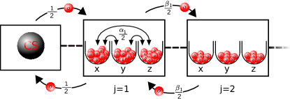
This completes the mapping of the equations of motion for operators of the CSM with large spin bath onto an effective Hamiltonian. This effective Hamiltonian acts on a four-dimensional impurity described by the matrices $M_{k}$ and $K_{k}$ and to a semi-infinite chain of bosons, see Fig. 1. The bosons act on the polynomials of the generalized Overhauser fields while the operator space of the central spin is represented by the impurity. Thus, it is now possible to represent every observable as a ket of this impurity model. For instance an operator acting solely on the central spin is a product state of the impurity state and the boson vacuum. In the course of the time evolution of the operator, contributions from the generalized Overhauser fields will appear, which correspond to the creation, annihilation, or the hopping of the bosons.

The first term of $\mathcal{H}_{\text{eff}}$, namely $\mathcal{H}_{\text{eff}}^{\text{CS}}$, creates and annihilates bosons at the head of the chain. Its coupling constant is $J_{\text{Q}}=1$, i.e., relatively large. The second term of $\mathcal{H}_{\text{eff}}$, namely $\mathcal{H}_{\text{eff}}^{\text{ch}}$, does not change the number of bosons, but lets them change flavor ($x,y,z$ or $1,2,3$, respectively, depending on the notation) on-site or combined with hops along the chain. Each change of flavor also changes the state of the impurity at the head of the chain. The scale of $\mathcal{H}_{\text{eff}}^{\text{ch}}$ is given by $\sqrt{\gamma}J_{\text{Q}}$. Hence, the corresponding rate is two to three orders of magnitude lower for $\gamma\approx 10^{-5}$ to $10^{-6}$ than the one induced by $\mathcal{H}_{\text{eff}}^{\text{CS}}$. This implies that $\mathcal{H}_{\text{eff}}^{\text{ch}}$ is a perturbation to $\mathcal{H}_{\text{eff}}^{\text{CS}}$, i.e., $\mathcal{H}_{\text{eff}}^{\text{ch}}$ is responsible for the slow, long-term dynamics.

III.6 Effective Hamilton operators for external magnetic fields

In this subsection, we point out how magnetic fields can be incorporated as well. First, we study the case where $h$ is acting on the central spin along the $\alpha$ direction. If the spin Hamiltonian is amended by the Zeeman term

$$\mathcal{H}^{\text{Z}}=-hS_{0}^{\alpha}$$ (46)

this translates straightforwardly to the amendment

$$\mathcal{H}_{\text{eff}}^{\text{Z}}=-hK_{\alpha}$$ (47)

of the effective Hamiltonian because only the operators of the central spins are relevant and the commutation of Pauli matrices is represented by the matrices $K_{\alpha}$. The Zeeman term for the central spin will be employed in the numerical evaluation below.

Second, we consider the action of a magnetic field in $\alpha$ direction on the spins of the bath. Motivated by the much lower nuclear magnetic moments, we denote the magnetic field by $zh$ where $z\approx 1/800$ takes the much lower effect of a magnetic field on the nuclear spins into account Beugeling et al. (2017). This means that we deal with the additional term $\mathcal{H}^{\text{nZ}}$ for the nuclear Zeeman effect

$$\mathcal{H}^{\text{nZ}}=-zh\sum_{i=1}^{N}S_{i}^{\alpha}.$$ (48)

Computing the corresponding Liouville operator yields

$$\mathcal{L}^{\text{nZ}}\vec{P}_{j}=iz\vec{h}\times\vec{P}_{j},$$ (49)

which translates to

$$\mathcal{L}^{\text{nZ}}{P}_{j}^{\alpha}=iz\sum_{\beta,\delta}\epsilon_{\alpha\beta\delta}h^{\beta}{P}_{j}^{\delta}.$$ (50)

Using again (as in the previous subsections) that the sequence of bath operators does not matter in leading order in $1/N_{\text{eff}}$, we obtain

$$[\mathcal{H}^{\text{nZ}},H_{n_{j,\alpha}}]=iz\sqrt{n_{j,\alpha}}H_{n_{j,\alpha}-1}\sum_{\beta,\delta}\epsilon_{\alpha\beta\delta}h^{\beta}{P}_{j}^{\delta}$$ (51)

and finally

$$\mathcal{L}^{\text{nZ}}(\sigma_{m}A^{\mathbold{n}})=iz\sigma_{m}\sum_{j=1}^{N_{\text{tr}}}\sum_{\alpha,\beta,\delta}\epsilon_{\alpha\beta\delta}\sqrt{n_{j,\alpha}}h^{\beta}{P}_{j}^{\delta}A_{\mathbold{\pi}(\mathbold{n},j,\alpha)}.$$ (52)

This allows us to express the Liouvillean of the nuclear Zeeman effect by annihilation and creation operators

$$\mathcal{H}_{\text{eff}}^{\text{nZ}} =-iz\sum_{j=1}^{N_{\text{tr}}}\sum_{\alpha,\beta,\delta=1}^{3}\epsilon_{\alpha\beta\delta}h^{\beta}a_{j,\alpha}^{\phantom{\dagger}}(a_{j,\delta}^{\phantom{\dagger}}+a_{j,\delta}^{\dagger})$$ (53a)

$$={-iz}\sum_{j=1}^{N_{\text{tr}}}\sum_{\alpha,\beta,\delta=1}^{3}\epsilon_{\alpha\beta\delta}h^{\beta}a_{j,\delta}^{\dagger}a_{j,\alpha}^{\phantom{\dagger}}.$$ (53b)

In passing to the second line, we used the antisymmetry of the Levi-Civita symbol. Note that the Hamiltonian $\mathcal{H}_{\text{eff}}^{\text{nZ}}$ has no effect on the central impurity so that no matrices $M_{\beta}$ or $K_{\beta}$ occur. We will not use this term in the numerical implementation below. For short times, it is not relevant due to the small value of $z$, but for longer times it does have an effect on higher correlations Fröhling and Anders (2017) and on quantum dots subject to pulses Beugeling et al. (2017); Jäschke et al. (2017).

Thus, magnetic fields acting on the central spin or on the bath spins can also be accounted for easily.

IV Comparison to other data

To establish the validity of the derived effective model in the limit $N_{\text{eff}}\to\infty$, we compare its results to quantitative results obtained by various established approaches which capture the temporal dependence up to a certain time and which can cope only with relatively small baths. Still, this is sufficient to see that the effective model reproduces the correct physics in the limit $N_{\text{eff}}\to\infty$.

The effective model of a semi-infinite bosonic chain coupled to a four-dimensional impurity can be simulated numerically. The spin-spin correlation in the original model

$$S(t):=\langle S^{z}_{0}(0)S_{0}^{z}(t)\rangle$$ (54)

is obtained in the effective model from the time evolution of the state $|3;\mathbold{0}\rangle\rangle$ where $\mathbold{0}=(0,0,0,\ldots)$ stands for the bosonic vacuum and $3$ stands for the third Pauli matrix, i.e., a particular state of the four-dimensional central impurity. Hence, we compute

$$S(t)=\frac{1}{4}\left\langle\left\langle 3;\mathbold{0}|\exp(-i\mathcal{H}_{\text{eff}}t)|3;\mathbold{0}\right\rangle\right\rangle.$$ (55)

Note that $S(t=0)=1/4$ as it has to be for the spin-spin autocorrelation in (54).

IV.1 Numerical implementation

For the present proof-of-principle, we do not implement a highly sophisticated code to compute the time dependence induced by $\mathcal{H}_{\text{eff}}$. We use a finite, truncated basis comprising the four states of the central impurity and a finite number of bosonic states given by the occupation numbers in the $3N_{\text{tr}}$-tuple $\mathbold{n}$. The resulting finite dimensional Schrödinger equation for the kets is an ordinary linear differential equation which is solved by a Runge-Kutta algorithm of fourth order. The starting vector is $|3;\mathbold{0}\rangle\rangle$. Finally, the scalar product is computed with respect to the bra $\left\langle\left\langle 3;\mathbold{0}\right|\right.$.

The key approximation in the implementation is the truncation of the maximum bosonic occupation for each site $j\leq N_{\text{tr}}$. We restrict the Hilbert space by means of the condition

$$\sum^{3}_{\alpha=1}n_{j,\alpha}<n_{\text{j;max}}.$$ (56)

Note that this restricts the total number of bosons at each site $j$ of the chain irrespective of their flavor $\alpha\in\{1,2,3\}$. This has turned out to be the most efficient way of local truncation.

The most important number is the threshold for the bosons at $j=1$ because it restricts how well the dominant $\mathcal{H}_{\text{eff}}^{\text{CS}}$ is represented. The other thresholds can be chosen significantly lower, see below. In practice, we build the basis iteratively by applying $\mathcal{H}_{\text{eff}}$ again and again. States which do not fulfil (56) for $j>1$ are truncated and the repeated application of $\mathcal{H}_{\text{eff}}$ is continued. For $j=1$, the recursive application of $\mathcal{H}_{\text{eff}}$ is stopped once (56) is violated. This procedure enhances the performance without changing the results noticeably up to the times for which the implementation provides reliable data.

Figure 2: Comparison of the analytical solution $S_{\text{fOver}}(t)$ for frozen Overhauser field in Eq. (57) to the numerical result obtained from $\mathcal{H}_{\text{eff}}^{\text{CS}}$ alone for various cutoffs $n_{\text{1;max}}$ of the occupation number.

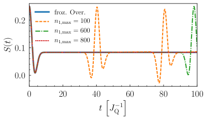
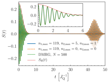
First, we consider $\mathcal{H}_{\text{eff}}^{\text{CS}}$ alone so that only $n_{\text{1;max}}$ matters. Physically, this means that the Overhauser field $\vec{B}$ is frozen, i.e., static. Then, the result can be obtained analytically either in a fully classical way Merkulov et al. (2002) or based on correlated fluctuations Stanek et al. (2013) as well. It reads

$$S_{\text{fOver}}(t)=\frac{1}{12}\left\{1+2\left[1-\frac{J_{\text{Q}}^{2}}{4}t^{2}\right]\exp\left[-\frac{J_{\text{Q}}^{2}}{8}t^{2}\right]\right\}$$ (57)

and it is suitable to check our numerical approach on the simplest level. In Fig. 2, the analytical result is compared to $S(t)$ obtained from $\mathcal{H}_{\text{eff}}^{\text{CS}}$ alone for various cutoffs $n_{\text{1;max}}$ in the occupation number. Clearly, the short-term behavior is perfectly reproduced and the constant plateau as well up to some threshold time $t_{\text{thresh}}$ at which a spurious revival of the initial correlation appears. This spurious revival occurs the later the larger the cutoff $n_{\text{1;max}}$ is chosen which underlines that it is a numerical effect due to the truncation of the Hilbert space.

We analyzed the scaling of the threshold time $t_{\text{thresh}}$ as function of $n_{\text{1;max}}$ and found that $t_{\text{thresh}}\propto\sqrt{n_{\text{1;max}}}$ with a prefactor between $3$ and $4$ for $J_{\text{Q}}=1$. This is actually expected for the approximation of time dependences on the basis of Hermite polynomials. Hence, we realize that the implementation using the occupation number representation is not very powerful for long times. But for the purposes of our present goal of a proof-of-principle comparison to other data this implementation is sufficient.

Next, we have to include the dynamics of the Overhauser field by increasing $N_{\text{tr}}$. We aim at comparisons up to $t=50/J_{\text{Q}}$ so that it turns out that $N_{\text{tr}}=3$ is sufficient. The corresponding limits for the occupation numbers $n_{\text{j;max}}$ for $j>1$ do not need to be chosen large because the dynamics of the Overhauser field is governed by the rate $\sqrt{\gamma}J_{\text{Q}}$ which is significantly smaller. These numbers can be determined self-consistently by increasing $n_{\text{j;max}}$ step by step till the result no longer depends on $n_{\text{j;max}}$. In this way, we arrive at $n_{\text{1;max}}=181,n_{\text{2;max}}=8$, and $n_{\text{3;max}}=1$. This triple will be used henceforth, if not denoted otherwise.

In contrast to the solution for a frozen Overhauser field, including the dynamics of the bath, i.e., of the Overhauser field, leads to a further decay of the autocorrelation function $S(t)$ such that $S(t\to\infty)<S(t=0)/3$ holds. Describing this dynamics of the bath quantum mechanically in the limit of very large $N_{\text{eff}}$ is a central goal of the present approach.

IV.2 Other approaches

We compare the data obtained from the effective Hamiltonian $\mathcal{H}_{\text{eff}}$ in (43) derived from the iterated equations of motion (iEoM) to data from three other techniques.

The first one is a fully classical simulation (classical) averaged over random Gaussian initial configurations. Previously, it was argued Chen et al. (2007) and shown that this approach approximates the quantum mechanical dynamics fairly well Stanek et al. (2013, 2014) and it can be efficiently used for large spin baths and large times Fauseweh et al. (2017). The spin baths studied below can easily be treated without further approximations. The data is averaged over $10^{8}$ initial configurations so that no statistical error is discernible.

The second one is the Bethe ansatz (BA). Although it is known since the early days of Gaudin Gaudin (1976, 1983) that the CSM is integrable and exactly solvable by Bethe ansatz, it has taken a long time till the tedious evaluation of the Bethe equations for larger systems has become possible Faribault and Schuricht (2013a). The treatment of the fully disordered initial state poses an additional challenge which has been solved by importance sampling Faribault and Schuricht (2013b). Here we use data already computed for Ref. Seifert et al., 2016 to test rigorous bounds for persisting correlations. The BA evaluated in the above cited fashion is very powerful in determining the dynamics for long times, but the bath sizes may not exceed 48 spins. Due to the stochastic evaluation the data has a relative error of about 5% Seifert et al. (2016).

The third technique is the time-dependent density-matrix renormalization group (DMRG). This approach is mostly used for one-dimensional problems, but it is also perfectly suited to treat star-like clusters as in the CSM Stanek et al. (2013). On the one hand, DMRG is powerful enough to deal with up to about 1000 spins in the bath. On the other hand, its caveat is that the growth in entanglement is so fast that only times up to about 30 to 50$J_{\text{Q}}^{-1}$ can be reached reliably. The parameters for the data shown below are the following. We keep $4096$ states in the DMRG sweeps and use the second order Trotter-Suzuki decomposition for the time propagation with a time step of $0.01J_{\text{Q}}^{-1}$. The dominant cause for the loss of accuracy is the discarded weight in the course of the time propagation. We stop the calculations if the accumulated discarded weight exceeds $0.001$.

We emphasize that the iEoM approach is tailored to capture quantum mechanical fluctuations of the central spin for a large number of effectively coupled spins $N_{\text{eff}}$. This is the relevant case to describe experiments on semiconductor quantum dots. But to gauge the introduced approach we use a rather small numbers of bath spins (18 to 48), which are still tractable with BA and DMRG in order to have exact results as reference.

IV.3 Results without external magnetic field

First, we focus on the CSM without external field. The motivation is twofold. Experimentally, spin noise has become a focus of experimental studies Crooker et al. (2010); Kuhlmann et al. (2013); Zapasskii et al. (2013); Dahbashi et al. (2014); Yang et al. (2014); Glasenapp et al. (2016) so that reliable theoretical investigations are called for. Theoretically, it turns out that the zero-field case represents a particular challenge because for finite fields expansions around isolated precessing spins work quite successfully Khaetskii et al. (2002, 2003); Coish and Loss (2004); Breuer et al. (2004); Fischer and Breuer (2007); Ferraro et al. (2008); Deng and Hu (2006, 2008); Coish et al. (2010); Barnes et al. (2012); Beugeling et al. (2016, 2017).

Figure 3: Comparison of results for the spin-spin correlation for given values of $\gamma=1/18$, cf. Eq. (3), in the zero-field CSM obtained by various approaches explained in the main text, see Sect. IV.2. The dashed line is the analytical result for frozen Overhauser field (57) depicted for reference. The behavior for very short times is indistinguishable in all approaches including the frozen Overhauser field. The upper panel shows the curves for a smaller total number $N$ of spins while the lower panel refers to a larger number $N$.

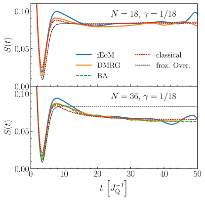
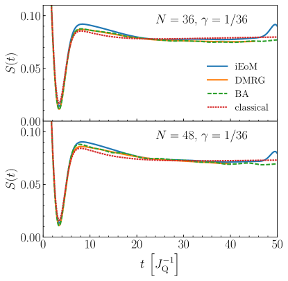
In Fig. 3 we included the static, frozen Overhauser formula (57) for comparison with the classical, the fully quantum mechanical, and the iEoM approach. In the upper panel, it appears that all approaches display the same long time behavior close to $S(t\to\infty)=S(0)/3$. But in the lower panel, it is obvious that the dynamics of the bath yields a lower autocorrelation $S(t\to\infty)<S(0)/3$. For a comprehensive rigorous discussion of this aspect we refer the reader to Refs. Uhrig et al., 2014; Seifert et al., 2016, which deal with persisting autocorrelations in the infinite time limit in the quantum CSM.

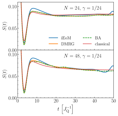
Figures 3, 4, and 5 depict a series of three decreasing values of $\gamma$ because the derived approach (iEoM) resides on an expansion in $1/N_{\text{eff}}\propto\gamma$. In each figure the upper panel shows the case of a lower value of the total number $N$ of bath spins. The lower panel shows data for a significantly larger $N$. At first glance, it can be stated that all the curves agree quite well and show the same qualitative behavior. The iEoM data shows some wiggles starting around $t=45J_{\text{Q}}^{-1}$ which can be attributed to the truncation of the basis. They could be suppressed by choosing larger $n_{\text{j;max}}$, but this enhances the required memory exponentially and the present calculation already used about 256 Gbytes of RAM. In addition, the wiggles tell us where the truncation effects show up so that it is instructive to see them.

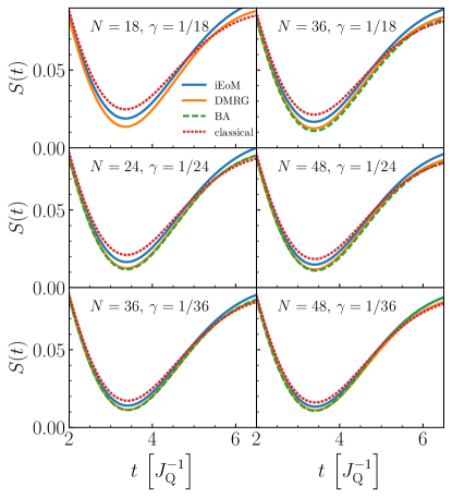
Since the initial dynamics leading to the dips around $t\approx 3.5J_{\text{Q}}^{-1}$ is very difficult to see in Figs. 3, 4, and 5, we include Fig. 6 where zooms of the dips are shown. From top to bottom, the parameter $\gamma$ decreases while from left to right the total number $N$ of spins increases.

Figure 4: Comparison of results for the spin-spin correlation for given values of $\gamma=1/24$, cf. Eq. (3), in the zero-field CSM obtained by various approaches. The upper panel shows the results for smaller $N$, the lower panel for larger $N$.

Comparing the data of the other approaches among them we see that the BA and the DMRG data almost coincide as it has to be because both approaches are numerically exact. By this we mean that in principle, using large enough resources, the results can be made arbitrarily accurate. The persisting deviations can be attributed to statistical errors in the BA evaluation which is based on importance sampling. They occur at shorter times but do not accumulate for longer times. The accuracy of the DMRG data is very high for short times, but deteriorates for longer times for three reasons. The first is the exponential growth of entanglement which cannot be captured anymore by the number of states kept beyond a certain time threshold. The second is the accumulated discarded weight in the temporal propagation of the state. The third is the accumulated errors due to the Trotter-Suzuki discretization. The main issue in the presented numerical data is discarded weight.

Figure 5: Comparison of results for the spin-spin correlation for given values of $\gamma=1/36$, cf. Eq. (3), in the zero-field CSM obtained by various approaches. The upper panel shows the results for smaller $N$, the lower panel for larger $N$.

The classical simulation represents an approximate treatment residing on very good arguments for the Overhauser field for large spin baths Chen et al. (2007); Stanek et al. (2013, 2014), but not for the central spin. Against this background, the proximity of the averaged classical result to the fully quantum mechanical calculations is remarkable.

Figure 6: Comparison of results for the spin-spin correlation for various values of $\gamma$ in the zero-field CSM obtained by various approaches. Here we focus on the initial dip. The left panels show the results for smaller $N$, the right panels for larger $N$. From top to bottom, the sequence of panels depicts data for decreasing values of $\gamma$.

Turning to the comparison of the iEoM results with the other data, one becomes aware that the effects are relatively small because all data are already close to one another. Yet, two trends catch the eye. First, the agreement of the iEoM curves with the DMRG and BA data becomes slowly better if at fixed $\gamma$ the total number $N$ of spins is increased. This effect can be assessed by comparing the upper panel with lower $N$ to the lower panel with larger $N$ in each of the three figures. This is a nice observation bearing in mind that experimentally $N$ is of the order or the number of atoms in the sample ($N\approx 10^{21}$ for a platelet with linear dimensions in the range of millimeters and a weight of $0.1$g), i.e., infinity for any practical purpose.

Figure 7: Comparison of results for the spin-spin correlation for given values of $\gamma=1/12$, cf. Eq. (3), in the zero-field CSM obtained by various approaches.

The second effect concerns the dependence on $\gamma$ and it is more pronounced. By inspecting the series of decreasing $\gamma$ from Fig.  3 via Fig. 4 to Fig.  5 or in Fig. 6 from top to bottom, one notes that the agreement becomes better and better. This was to be expected because the approach as derived above resides on the leading behavior in an expansion in $\gamma$. Hence, the numerical data strongly corroborates the validity of the introduced approach.

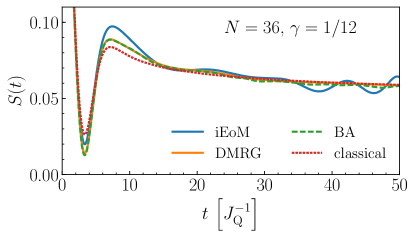
In order to underline this aspect further, Fig. 7 depicts the result for a large value of $N$, but also a large value of $\gamma$. This figure is to be compared to the upper panel of Fig. 5 which shows data for the same $N$, but for a three times smaller $\gamma$. Clearly, the results for smaller $\gamma=1/36$ agree significantly better than the results for $\gamma=1/12$. We emphasize again that the experimentally relevant values in quantum dots are of the order of $\gamma\approx 10^{-5}$ or even smaller. Hence, one can expect that the mapping of the CSM to an impurity in a bosonic bath is extremely accurate and captures all essential physics in the CSM relevant for semiconductor quantum dots.

It is interesting that in the range around $t\approx 10J_{\text{Q}}^{-1}$ the deviations of the iEoM curves to the fully quantum mechanical results are larger than for longer times where the agreement is much better. We attribute this observation to the fact that the neglected terms in the limit $\gamma\to 0$ are of order $\gamma$ relative to the leading order. For $\gamma=0$, only the frozen Overhauser dynamics (57) remains which is sizeable up to $t\approx 10J_{\text{Q}}^{-1}$, but completely flat and featureless beyond this time. Hence, in the time regime up to $t\approx 10J_{\text{Q}}^{-1}$ the corrections are of order $\gamma$. However, beyond this temporal regime, the dynamics is governed by $\mathcal{H}_{\text{eff}}^{\text{ch}}$ which is of order $\sqrt{\gamma}J_{\text{Q}}$. Hence, for longer times the neglected corrections are of order $\gamma^{3/2}$ and thus even smaller.

Still, further support for the above promising conclusions would be desirable, for instance for higher order correlations Press et al. (2010); Bechtold et al. (2016); Fröhling and Anders (2017) and for CSMs subject to pulses Greilich et al. (2006, 2007); Beugeling et al. (2016, 2017); Jäschke et al. (2017). In the present paper, we focused on the autocorrelation of the central spin in order to establish the mapping. But calculating other quantities such as higher order correlations is possible and cannot be done by classical means since the sequence of operators of the central spin matters.

IV.4 Results with external magnetic field

In the previous subsection we focused on the CSM without external field for experimental and theoretical reasons. Yet it is, of course, important to illustrate that the advocated iEoM approach also works with finite fields. So we extend the effective Hamiltonian $\mathcal{H}_{\text{eff}}$ in (43) by the dominant Zeeman term for the central spin in $x$-direction given in (47) and solve the ensuing differential equations in time.

Figure 8: Spin-spin correlation from iEoM for finite magnetic fields along $S^{x}$. The spin bath is infinite ($N=\infty$) with parameter $\gamma=0.01$ corresponding to $N_{\text{eff}}=200$ effectively coupled spins. The truncation of the bosonic Hilbert space is characterized by $n_{\text{1;max}}=51,n_{\text{2;max}}=2$, and zero otherwise.

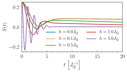
From numerical results Hackmann and Anders (2014), we expect that the Larmor precessions are governed by a frequency which is altered from the case of isolated spins where it is given by the magnetic field $h$. Due to the coupling to the bath the energy scale $J_{\text{Q}}$ enters yielding a shifted Larmor frequency

$$\omega_{\text{L}}=\sqrt{h^{2}+J_{\text{Q}}^{2}/2}.$$ (58)

This implies that small fields $h\ll J_{\text{Q}}$ hardly show any effect. Clearly, this is reproduced in Fig. 8 for $h=0.1J_{\text{Q}}$. Only above $h\approx 0.5J_{\text{Q}}$ a sizable effect sets in. True oscillations set in only above $h\approx 5J_{\text{Q}}$ in accordance with what was observed previously Stanek et al. (2014). For such large magnetic fields one discerns an oscillation bounded by an envelope function. This envelope function results from the Gaussian fluctuations of the Overhauser field $\vec{B}$ along the direction of the external magnetic field. Since the Fourier transform of a Gaussian distribution of Larmor frequencies is again a Gaussian in time, the envelope function is given by Merkulov et al. (2002); Stanek et al. (2014); Hackmann and Anders (2014)

$$S_{\text{H}}(t)=\frac{1}{4}\exp\left(-\frac{J_{\text{Q}}^{2}}{8}t^{2}\right).$$ (59)

If the distribution of the Overhauser field is squeezed it is indeed possible to extend the coherence Gravert et al. (2016). Alternatively, projective measurements help to maintain the central spin polarization Klauser et al. (2008).

Figure 9: Spin-spin correlation from iEoM for a magnetic field $h=10J_{\text{Q}}$ along $S^{x}$. The spin bath is infinite ($N=\infty$) with parameter $\gamma=0.01$ corresponding to $N_{\text{eff}}=200$ effectively coupled spins. The truncation of the bosonic Hilbert space is characterized by the numbers given in the legend. The DMRG data shown for reference are obtained for the same $\gamma$ and $N=500$. The envelope $S_{\text{H}}(t)$ is given by (59). The inset zooms into the region of the Larmor oscillations for clarity.

The excellent description of the decay of the Larmor precession by the envelope (59) is illustrated in Fig. 9. In addition, this figure illustrates effects of the finite truncation of the bosonic Hilbert space. The spurious revival can be pushed to larger times for larger $n_{\text{1;max}}$. Note that $n_{\text{2;max}}$ appears to be rather unimportant. This is so because the signal has vanished already on short time scales so that the dynamics of the Overhauser bath barely plays a role.

We stress that prior to the spurious revival the data obtained by the derived iEoM agrees perfectly well with the DMRG data included for comparison. This underlines that the iEoM approach not only works nicely in the zero-field case, but also at finite magnetic fields. In contrast to DMRG, the iEoM approach allows one to tackle much larger values of $N_{\text{eff}}\propto 1/\gamma$ in the limit $N=\infty$.

V Conclusions and Outlook

Motivated by the importance of systems of a single spin coupled to large baths of spins in quantum dots Merkulov et al. (2002); Schliemann et al. (2003); Hanson et al. (2007); Coish and Baugh (2009); Fischer and Loss (2009); Urbaszek et al. (2013); Ribeiro and Burkard (2013); Warburton (2013); Chekhovich et al. (2013), but also in NV-centers in diamond Jelezko and Wrachtrup (2006) or in generic NMR studies Álvarez et al. (2010), we investigated the quantum mechanical central spin model in the limit of large numbers $N_{\text{eff}}$ of bath spins. In quantum dots, $N_{\text{eff}}$ can be as large as $10^{5}$ to $10^{6}$ and around NV-centers and in large organic molecules the number of effectively coupled spins still ranges from 10 to 100.

Theoretically, we posed ourselves the question whether there is a well-defined limit $N_{\text{eff}}\to\infty$ and if so, whether the system becomes classical in this limit Chen et al. (2007); Stanek et al. (2013, 2014).

We started from the equations of motion for the spin operators, employed a suitable scalar product for operators Kalthoff et al. (2017), and used the observation that traces over infinite sums of spin operators can be computed from classical Gaussian correlations Seifert et al. (2016). In this way, we mapped the operator dynamics in the central spin model in the limit $N_{\text{eff}}\to\infty$ to the dynamics of states in an effective quantum model with a four-dimensional central impurity coupled to a bosonic bath without further interaction. The four-dimensional impurity represents the possible operators for the central spin. The bosons in the bosonic bath represent the collective spin degress of freedom in the large spin bath. Hence, a well-defined limit $N_{\text{eff}}\to\infty$ has been established.

We find it very remarkable that the analytic treatment of the limit $N_{\text{eff}}\to\infty$ does not make the system completely classical, but keeps its quantumness in the effective Hamiltonian $\mathcal{H}_{\text{eff}}$. Yet, the numerical data obtained from the averaged classical calculation, from the numerically exact approaches, and from the iEoM approach are very close to one another. The treatment of external magnetic fields is also possible. This holds for the central spin, but also for the relevant nuclear Zeeman terms Beugeling et al. (2017); Jäschke et al. (2017).

The derived mapping has two fundamental advantages: (i) It paves the way to the quantum mechanical treatment of very large spin baths which cannot be tackled otherwise at all. (ii) It enables the treatment of the central spin model by techniques which could so far not be used, for instance any approach conceived to deal with impurities coupled to interaction-free bosonic baths.

We tested the results obtained by the iEoM approach for smaller spin baths with 18 to 48 spins where reliable results obtained by established techniques are available. In this way, we verified the validity of the analytic arguments used in the derivation. The results are remarkably close to the numerically exact reference data, although the relatively low numbers of bath spins are disadvantageous for the introduced approach to work perfectly. The agreement improved for larger spin baths corroborating the derivation based on an expansion in $1/N_{\text{eff}}$.

Moreover, the good agreement for baths of moderate size suggests that the application of the iEoM approach is already fruitful for smaller spin baths as they arise for NV centers or in large molecules.

In cases of larger spin baths, the approach is expected to yield highly accurate results where other methods can not be applied at all. Thus the iEoM allows for investigations of quantum effects beyond classical descriptions in the regime of large spin baths. It has been the main goal of the present paper to derive such a theoretical technique.

Furthermore, the present treatment can be extended in a straightforward manner to larger bath spins, for instance $S=3/2$, which is the relevant case in GaAs Beugeling et al. (2017). To this end, only the variance of the Gaussian distributions has to be adapted.

We point out that the numerical implementation of the mapped model is not yet pushed to its limits. Further improvements are called for in order to reach longer times. This is crucial to describe many experiments, for example for measurements of higher order correlations Press et al. (2010); Bechtold et al. (2016); Fröhling and Anders (2017) or for quantum dots prepared in non-equilibrium states by intricate pulsing Greilich et al. (2006, 2007); Beugeling et al. (2016, 2017); Jäschke et al. (2017).

The route to follow to reach the necessary improvement is to exploit the significant difference in dynamics induced by the Hamiltonian part $\mathcal{H}_{\text{eff}}^{\text{CS}}$ and by the Hamiltonian part $\mathcal{H}_{\text{eff}}^{\text{ch}}$ where the rate of changes induced by the latter is smaller by a factor $1/\sqrt{N_{\text{eff}}}$. Hence, one should treat $\mathcal{H}_{\text{eff}}^{\text{CS}}$ exactly by choosing a representation in which it is diagonal. Such implementations are left for future research.

Appendix A Orthonormality of the generalized Overhauser fields

The fact that we orthonormalized the polynomials according to (11a) allows us to conclude that the components of the generalized Overhauser fields $\vec{P}_{j}$ are pairwise orthonormal with respect to the Frobenius scalar product (7) as well. For $j,k\in\{1,2,\ldots,N_{\text{tr}}\}$ and $\alpha,\beta\in\{x,y,z\}$ we obtain

$$\left\langle\left\langle{P}_{j}^{\alpha}\left|{P}_{k}^{\beta}\right.\right\rangle\right\rangle=$$

$$\quad=\frac{1}{2^{N-1}}\text{Tr}\left(\sum_{n,m=1}^{N}p_{j}(J_{n})p_{k}(J_{m})S_{n}^{\alpha}S_{m}^{\beta}\right)$$ (60a)

$$\quad=\frac{1}{2^{N-1}}\sum_{n,m=1}^{N}p_{j}(J_{n})p_{k}(J_{m})\underbrace{\text{Tr}\left(S_{n}^{\alpha}S_{m}^{\beta}\right)}_{2^{N-1}\delta_{nm}\delta_{\alpha\beta}}$$ (60b)

$$\quad=\sum_{n=1}^{N}p_{j}(J_{n})p_{k}(J_{n})\delta_{\alpha\beta}$$ (60c)

$$\quad=\delta_{jk}\delta_{\alpha\beta}$$ (60d)

which was to be proven.

Appendix B Irrelevance of commutators in the limit $N_{\text{eff}}\to\infty$

Here we provide an example that commutators represent subleading corrections to the scalar products of the products of generalized Overhauser fields. In order to keep the example transparent we consider the simplest commutator of two linear fields

$$[P^{\alpha}_{m},P^{\beta}_{l}] =\sum_{k,j=1}^{N}p_{m}(J_{k})p_{l}(J_{j})4[S^{\alpha}_{k},S^{\beta}_{j}]$$ (61a)

$$=\sum_{i=1}^{N}4p_{m}(J_{k})p_{l}(J_{k})i\sum_{\delta}\epsilon_{\alpha\beta\delta}S^{\delta}_{k}$$ (61b)

$$=:I^{\delta}.$$ (61c)

Next, we consider the norms of the involved operators. The generalized Overhauser fields $P^{\alpha}_{k}$, $P^{\beta}_{l}$ are normalized to unity by construction. But the scalar product of $I^{\delta}$ is of order $1/N_{\text{eff}}$ because each factor $p_{m}(J_{k})$ and $p_{l}(J_{i})$ is of order $1/\sqrt{N_{\text{eff}}}$. Hence, the summation over all bath spins in $\left\langle\left\langle I^{\delta}|I^{\delta}\right\rangle\right\rangle$ sums $N_{\text{eff}}$ terms, each of which proportional to $p_{m}(J_{k})^{2}p_{l}(J_{k})^{2}$ and hence of order $1/N_{\text{eff}}^{2}$. So, the scalar product of $I_{\delta}$ is of order $1/N_{\text{eff}}$ and hence subleading relative to the contributions resulting from products of the generalized Overhauser fields.

The above example illustrates the statement from the main text that the sequence of the generalized Overhauser fields in the terms of the operator basis does not matter for $N_{\text{eff}}\to\infty$.

Appendix C Calculation of $T_{1}$ and $T_{2}$

In order to obtain $T_{1}$ in Eq. (35), we compute

$$\mathcal{L}\sigma_{m}=$$ (62)

$$\left\{\begin{array}[]{ll}0&\text{if}\;m=0\\ \frac{i}{2}{\sigma}_{m+1}{P}_{1}^{m-1}-\frac{i}{2}{\sigma}_{m-1}{P}_{1}^{m+1}&\text{if}\;m\in\{1,\,2,\,3\},\end{array}\right.$$ (65)

where the indices for finite $m$ must be understood in a cyclic sense, i.e., for $m=1$ the decremented $m-1$ means $m-1=3$ and for $m=3$ the incremented $m+1$ means $m+1=1$. If we use the result (62) to compute the term $T_{1}$ for $\mathcal{L}(\sigma_{m}A^{\mathbold{n}})$ we obtain

$$T_{1}[\mathcal{L}(\sigma_{m}A^{\mathbold{n}})]=$$

$$\quad\frac{i}{4}\left(\sigma_{m+1}\{{P}_{1}^{m-1},A^{\mathbold}{n}\}-\sigma_{m-1}\{{P}_{1}^{m+1},A^{\mathbold}{n}\}\right).$$ (66)

The multiplication with ${P}_{1}^{m\pm 1}$ modifies the index of the Hermite polynomials $H_{n}({P}_{1}^{m\pm 1})$ according to (27a). This can be concisely expressed by creation and annihilation operators as is common in the analytic treatment of the eigen wave functions of the harmonic oscillator.

In order to address $T_{2}$ in Eq. (38), we consider terms of the type

$$\mathcal{L}H_{n_{j,\alpha}}({P}_{j}^{\alpha})=[\mathcal{H},H_{n_{j,\alpha}}({P}_{j}^{\alpha})].$$ (67)

First, we compute the application of the Liouville operator to the component of a generalized Overhauser field ${P}_{j}^{\alpha}$. A straightforward calculations shows that (12) implies

$$\mathcal{L}\vec{P}_{j}=-i\vec{S}_{0}\times\left(\beta_{j}\vec{P}_{j+1}+\alpha_{j}\vec{P}_{j}+\beta_{j-1}\vec{P}_{j-1}\right)$$ (68)

with the coefficients $\alpha_{j}$ and $\beta_{j}$. The coefficients $\beta_{0}:=0$ and $\beta_{N_{\text{tr}}}:=0$ are defined to vanish. If we use the definition of $R_{j}^{\delta}$ in (36) we can express the outer product in (68) using the Levi-Civita symbol $\epsilon_{\alpha\beta\delta}$

$$\mathcal{L}{P}_{j}^{\alpha}=-i\sum_{\beta,\delta=1}^{3}\epsilon_{\alpha\beta\delta}S_{0}^{\beta}R_{j}^{\delta}.$$ (69)

In order to treat the general case in (67) we combine (69) with the operator relation

$$[A,f(B)] =\frac{\partial f(B)}{\partial B}[A,B].$$ (70)

The latter requires that $[B,[A,B]]=0$ which does not hold generally. But here we can safely assume commutativity because the sequence of bath operators does not matter in leading order in $1/N_{\text{eff}}$. In this way, we arrive at

$$[\mathcal{H},H_{n_{j,\alpha}}] =-iH_{n_{j,\alpha}}^{\prime}\sum_{\beta,\delta=1}^{3}\epsilon_{\alpha\beta\delta}S_{0}^{\beta}R_{j}^{\delta}$$ (71a)

$$=-i\sqrt{n_{j,\alpha}}H_{n_{j,\alpha}-1}\sum_{\beta,\delta=1}^{3}\epsilon_{\alpha\beta\delta}S_{0}^{\beta}R_{j}^{\delta}.$$ (71b)

Hence, we have to decrement the degree of the Hermite polynomial $H_{n_{j,\alpha}}$.

All other Hermite polynomials are not affected in this step and remain unaltered. This is precisely what the decrementing mapping $\mathbold{\pi}(\mathbold{n},j,\alpha)$ defined in Eq. (37) expresses. In this way, we arrive at the final result for the product of Hermite polynomials as it appears in $A_{\mathbold}{n}$

$$[\mathcal{H},A_{\mathbold}{n}] =-i\sum_{j=1}^{N_{\text{tr}}}\sum_{\alpha=1}^{3}\sqrt{n_{j,\alpha}}A_{\mathbold{\pi}(\mathbold{n},j,\alpha)}\sum_{\beta,\delta=1}^{3}\epsilon_{\alpha\beta\delta}S_{0}^{\beta}R_{j}^{\delta}.$$ (72)

Finally, we combine this finding with the Pauli matrices for the central spin and obtain

$$T_{2}[\mathcal{L}(\sigma_{m}A_{\mathbold{n}})]=\frac{-i\sigma_{0}}{2}\sum_{j=1}^{N_{\text{tr}}}\sum_{\alpha,\delta=1}^{3}\epsilon_{\alpha m\delta}\sqrt{n_{j,\alpha}}R^{\delta}_{j}A_{\mathbold{\pi}(\mathbold{n},j,\alpha)}$$ (73a)

for $$m\in\{1,2,3\} \{\sigma_{m},\sigma_{\beta}\}=2\delta_{m\beta} m,\beta\in\{1,2,3\} m=0$$ where we used that if . For , we obtain

$$T_{2}[\mathcal{L}(\sigma_{0}A^{\mathbold{n}})]=\frac{-i}{2}\sum_{j=1}^{N_{\text{tr}}}\sum_{\alpha,\beta,\delta=1}^{3}\epsilon_{\alpha\beta\delta}\sqrt{n_{j,\alpha}}\sigma_{\beta}R^{\delta}_{j}A_{\mathbold{\pi}(\mathbold{n},j,\alpha)},$$ (73b)

where we used $\{\sigma_{0},\sigma_{\beta}\}=2\sigma_{\beta}$.

Appendix D Commutation and Anticommutation Matrices

The anticommutation of the operators of the central spin with $\sigma_{k}$ is described by the matrices $M_{k}$. Their matrix elements are defined in Eq. (41). The matrices read

$${M}_{1} =\begin{pmatrix}0&1&0&0\\ 1&0&0&0\\ 0&0&0&0\\ 0&0&0&0\end{pmatrix},$$ (74a)

$${M}_{2} =\begin{pmatrix}0&0&1&0\\ 0&0&0&0\\ 1&0&0&0\\ 0&0&0&0\end{pmatrix},$$ (74b)

$${M}_{3} =\begin{pmatrix}0&0&0&1\\ 0&0&0&0\\ 0&0&0&0\\ 1&0&0&0\end{pmatrix}.$$ (74c)

The commutation of the operators of the central spin with $\sigma_{k}$ is described by the matrices $K_{k}$. Their matrix elements are defined in Eq. (42). The matrices read

$${K}_{1} =\begin{pmatrix}0&0&0&0\\ 0&0&0&0\\ 0&0&0&i\\ 0&0&-i&0\end{pmatrix},$$ (75a)

$${K}_{2} =\begin{pmatrix}0&0&0&0\\ 0&0&0&-i\\ 0&0&0&0\\ 0&i&0&0\end{pmatrix},$$ (75b)

$${K}_{3} =\begin{pmatrix}0&0&0&0\\ 0&0&i&0\\ 0&-i&0&0\\ 0&0&0&0\end{pmatrix}.$$ (75c)

Appendix E Diagonalization of $\mathcal{H}_{\text{eff}}^{\text{ch}}$

Instead of considering a semi-infinite chain with hopping bosons as described by $\mathcal{H}_{\text{eff}}^{\text{ch}}$ in Eq. (45), it can be advantageous to restrict it to local processes only. Then the system resembles a bath of bosons with flavor $x,y,z$ connected to the central four-dimensional impurity. This mapping is obtained by defining vectors of the bosonic operators

$$\mathbold{a}_{\alpha}^{\phantom{\dagger}} :=\begin{pmatrix}{a}_{1,\alpha}^{\phantom{\dagger}},&{a}_{2,\alpha}^{\phantom{\dagger}},&\dots,&{a}_{L,\alpha}^{\phantom{\dagger}}\\ \end{pmatrix}^{\text{T}},$$ (76a)

$$\mathbold{a}_{\alpha}^{\dagger} :=\begin{pmatrix}{a}_{1,\alpha}^{\dagger},&{a}_{2,\alpha}^{\dagger},&\dots,&{a}_{L,\alpha}^{\dagger}\end{pmatrix},$$ (76b)

where $\mathbold{a}_{\alpha}^{\phantom{\dagger}}$ is a column vector while $\mathbold{a}_{\alpha}^{\dagger}$ is a row vector. With these definitions and the tridiagonal matrix $\mathbold{T}$ from (17) the chain Hamilton can be denoted concisely

$$\mathcal{H}_{\text{eff}}^{\text{ch}}=\frac{i}{2}\sum_{\alpha,\beta,\delta}\epsilon_{\alpha\beta\delta}{M}_{\beta}\ \mathbold{a}_{\delta}^{\dagger}\mathbold{T}\mathbold{a}_{\alpha}^{\phantom{\dagger}}.$$ (77)

The tridiagonal matrix $\mathbold{T}$ is real and symmetric so that it can be diagonalized by a real orthogonal matrix $\mathbold{Q}$

$$\mathbold{D}=\mathbold{Q}^{\dagger}\mathbold{T}\mathbold{Q}$$ (78)

yielding the diagonal matrix $\mathbold{D}$ which has the eigen values $\varepsilon_{j}$ on its diagonal. Then the transformed vectors of annihilation and creation operators $d_{j,\alpha}^{\phantom{{\dagger}}}$ and $d_{j,\alpha}^{\dagger}$ are given by

$$\mathbold{d}_{\alpha} :=\mathbold{Q}^{\dagger}\mathbold{a}_{\alpha}^{\phantom{\dagger}},$$ (79a)

$$\mathbold{d}_{\alpha}^{\dagger} :=\mathbold{a}_{\alpha}^{\dagger}\mathbold{Q}.$$ (79b)

They allow us to express the Hamiltonian $\mathcal{H}_{\text{eff}}^{\text{ch}}$ in an (almost) diagonal form

$$\mathcal{H}_{\text{eff}}^{\text{ch}}=\frac{i}{2}\sum_{\alpha,\beta,\delta}\epsilon_{\alpha\beta\delta}{M}_{\beta}\sum_{j=1}^{N_{\text{tr}}}\varepsilon_{j}\ {d}_{j,\delta}^{\dagger}{d}_{j,\alpha}^{\phantom{\dagger}}.$$ (80)

The missing piece is the transformed Hamiltonian $\mathcal{H}_{\text{eff}}^{\text{CS}}$ which is obtained by inserting the inverses of Eqs. (79) into (44a)

$$\mathcal{H}_{\text{eff}}^{\text{CS}}=\frac{1}{2}\sum_{\alpha}K_{\alpha}\sum_{j=1}^{N_{\text{tr}}}Q_{1,j}\left(d_{j,\alpha}^{\phantom{\dagger}}+d_{j,\alpha}^{\dagger}\right),$$ (81)

where we used the fact that $\mathbold{Q}$ is real so that no complex conjugation needs to be taken into account. For simplicity, one may make all $Q_{1,j}\geq 0$ by choosing the signs of the $d_{j,\alpha}$ appropriately. We highlight this fact because it allows us to point out the relation to the spectral density approach introduced in Ref. Fauseweh et al., 2017. The exponential discretization of the spectral densities relevant for the set of couplings $J_{i}$ directly provides energies $\varepsilon_{j}$ and weights $W_{j}$. The square roots of the weights determine the coefficients $Q_{1,j}=\sqrt{W_{j}}$.

Eventually, Eqs. (80) and (81) together define the complete effective Hamiltonian for the central spin model with large spin baths. This effective model comprises a central four-dimensional impurity coupled to a surrounding bath of bosonic sites $j$, where bosons of three flavors are exchanged with one another.