Fermionic reaction coordinates and their application to an autonomous Maxwell demon in the strong coupling regime

Abstract

We establish a theoretical method which goes beyond the weak coupling and Markovian approximations while remaining intuitive, using a quantum master equation in a larger Hilbert space. The method is applicable to all impurity Hamiltonians tunnel-coupled to one (or multiple) baths of free fermions. The accuracy of the method is in principle not limited by the system-bath coupling strength, but rather by the shape of the spectral density and it is especially suited to study situations far away from the wide-band limit. In analogy to the bosonic case, we call it the fermionic reaction coordinate mapping. As an application we consider a thermoelectric device made of two Coulomb-coupled quantum dots. We pay particular attention to the regime where this device operates as an autonomous Maxwell demon shoveling electrons against the voltage bias thanks to information. Contrary to previous studies we do not rely on a Markovian weak coupling description. Our numerical findings reveal that in the regime of strong coupling and non-Markovianity, the Maxwell demon is often doomed to disappear except in a narrow parameter regime of small power output.

I Introduction

Many problems in quantum transport are modeled by an impurity Hamiltonian $H_{\text{imp}}$ linearly coupled to a bath of free fermions described via

$$H=H_{\text{imp}}+\sum_{k}(t_{k}dc_{k}^{\dagger}+h.c.)+\sum_{k}\epsilon_{k}c_{k}^{\dagger}c_{k}.$$ (1)

Here, $c_{k}^{(\dagger)}$ annihilates (creates) a fermion of energy $\epsilon_{k}$ in the bath, which is tunnel-coupled with complex amplitude $t_{k}$ to the system via a fermionic annihilation (creation) operator $d^{(\dagger)}$ of the system. The actual physical system under study is described by $H_{\text{imp}}$, which could be one (or multiple) quantum dots, molecules in mechanically controllable break junctions or nano-electro-mechanical systems, among other possible impurity systems.

To treat such systems theoretically, various approximate or formally exact techniques have been developed, such as quantum master equations (MEs) Breuer and Petruccione (2002); Schaller (2014); de Vega and Alonso (2017), the formalism of nonequilibrium Green’s functions Stefanucci and van Leeuwen (2013) or renormalization group techniques Bulla et al. (2008). Whereas MEs easily allow to treat interactions in the impurity even under nonequilibrium situations, their use is limited to the weak coupling, Markovian and high temperature (“sequential tunneling”) regime. Green’s functions can overcome the latter problem, but have difficulties to treat interacting impurities (for instance, due to Coulomb forces). Whereas this problem can be tackled by using numerical renormalization group approaches, they in turn are hard to apply far away from equilibrium.

In the first half of this article (Sec. II), we will introduce a technique which lies “in between” these approaches. It allows to some extent to overcome the limitations of the standard perturbative approach commonly applied to obtain a ME while still retaining a description in terms of a ME such that interactions and nonequilibrium situations can be conveniently treated. The price to pay is an enlarged Hilbert space, in which a suitable redefined impurity Hamiltonian $\tilde{H}_{\text{imp}}$ includes particularly choosen dominant degrees of freedom from the bath, which we will call fermionic reaction coordinates (RCs). In the context of linear bosonic reservoirs (Caldeira-Leggett or Brownian motion models), this technique has a longer tradition Garg et al. (1985). It has found various applications in the theory of open quantum systems Jean et al. (1992); May et al. (1993); Pollard and Friesner (1994); Wolfseder and Domcke (1996); Wolfseder et al. (1998); Hartmann et al. (2000); Thoss et al. (2001); Cederbaum et al. (2005); Hughes et al. (2009a, b); Martinazzo et al. (2011a, b); Iles-Smith et al. (2014); Huh et al. (2014); Bonfanti et al. (2015); Iles-Smith et al. (2016) and it is also closely related to the “time evolving density matrix using orthogonal polynomials algorithm” (TEDOPA) Prior et al. (2010); Chin et al. (2010); Woods et al. (2014, 2015); Woods and Plenio (2016); Rosenbach et al. (2016). We remark that, although it shares many similarities with the bosonic case, the RC mapping was not studied for fermionic reservoirs before. In addition, our article adds additional insights to the recent attempts to find a meaningful thermodynamic description beyond the weak coupling and Markovian regime Esposito et al. (2010, 2015a, 2015b); Bruch et al. (2016); Seifert (2016); Strasberg et al. (2016); Talkner and Hänggi (2016); Kato and Tanimura (2016); Cerrillo et al. (2016); Whitney (2016); Newman et al. (2017); Jarzynski (2017); Miller and Anders (2017); Strasberg and Esposito (2017); Perarnau-Llobet et al. (2017); Mu et al. (2017); Haughian et al. (2018); Restrepo et al. (2017). In particular, our work shows that techniques based on a redefined system-bath partition using RC mappings Strasberg et al. (2016); Newman et al. (2017); Strasberg and Esposito (2017); Restrepo et al. (2017) turn out to be useful for fermionic reservoirs, too.

In the second half of the article (Secs. III and IV) we make use of our new method to study two (spinless) Coulomb-coupled quantum dots in contact with three heat reservoirs. This setup is raising increasing attention within the context of quantum thermodynamics, as it provides a prototypical example of a thermoelectric device transporting electrons against a potential bias due to an energetic flow from a hot to a cold bath Sánchez and Jordan (2015); Benenti et al. (2017). It is well-studied in the weak-coupling and Markovian regime, theoretically Sánchez and Büttiker (2011); Strasberg et al. (2013) as well as experimentally Hartmann et al. (2015); Thierschmann et al. (2015). Moreover, Ref. Strasberg et al. (2013) identified necessary conditions which guarantee that this device can be interpreted as an autonomous Maxwell demon (MD), i.e., a device which is capable of extracting work (in this case by charging a battery) due to a clever way of processing information. From this perspective the device was further studied theoretically Horowitz and Esposito (2014); Kutvonen et al. (2015) and experimentally Koski et al. (2015).

Unfortunately, the study in Ref. Strasberg et al. (2013) has revealed that a proper operation of the device as a MD requires a strong coupling to a cold reservoir and structured (i.e., non-Markovian) spectral densities for the hot reservoirs. These three requirements challenge the usual range of validity of a ME description, but the question whether the transparent interpretation of a MD also holds under these conditions has not been answered yet. By using the method of fermionic RCs, we will indeed show that the device can still be interpreted as a MD, albeit in a very narrow parameter regime restricted to low power output. Our results are also in qualitative agreement with a recent study Walldorf et al. (2017) where cotunneling effects were taken into account. Another complementary paper studies the impact of strong coupling effects for non-autonomous, i.e., measurement-based, feedback loops on the thermodynamic performance of a MD Schaller et al. (2017).

II Fermionic reaction coordinates

In this section we develop the theory of fermionic reaction coordinates (RCs), which is useful to explore the physics of open systems beyond the weak coupling, Markovian and high temperature assumption. Technically speaking, this mapping is a unitary transformation applied to the bath Hamiltonian, which allows to separate out a particular degree of freedom in the bath, called the RC. The details of this transformation are reported in Sec. II.1.

The hope is then that the original impurity together with the RC is only weakly coupled to a Markovian residual bath such that it is possible to apply standard master equation (ME) procedures to this redefined system-bath partition. Whether this is possible is case-dependent and will be discussed in Sec. II.2.

To make the paper self-contained, we also give a short review in Appendix A of the ME approach including the definition of energy and particle currents, which we will use in the second part of this paper. Furthermore, in Appendix B we benchmark the fermionic RC method against the exact solution of the Fano-Anderson model (also known as single electron transistor).

II.1 The mapping

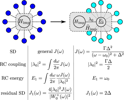
The mapping will work whenever it is allowed to describe the interaction between an arbitrary impurity Hamiltonian $H_{\text{imp}}$ and the fermionic reservoir as in Eq. (1). An important quantity in the study of such open systems is the spectral density (SD) (also called hybridization function) of the bath, which is defined as

$$J(\omega)\equiv 2\pi\sum_{k}|t_{k}|^{2}\delta(\omega-\epsilon_{k}).$$ (2)

It contains the complete information about the way in which the bath is coupled to the system and will be of central importance in the following.

For mathematical rigour one often demands that $J(\omega)$ is strictly greater than zero for $\omega\in[\omega_{L},\omega_{R}]$ and zero outside this interval where $\omega_{L}<\omega_{R}\in\mathbb{R}$ are referred to as cutoff frequencies Martinazzo et al. (2011a). However, as long as all quantities converge, our equations also remain valid if the SD decays only exponentially or polynomially. Convergence problems for infinite cutoff frequencies arise only when the mapping is applied iteratively (see below). Furthermore, gapped SDs (having support only at disconnected intervals) can be treated by applying this mapping to each sub-SD separately.

For later reference, we start by considering the Heisenberg equation of motion for $d$ and $c_{k}$ (suppressing the time-dependence on all operators and setting $\hbar\equiv 1$ throughout):

$$\dot{d} =i[H_{\text{imp}},d]+i\sum_{k}t_{k}^{*}c_{k},$$ (3)

$$\dot{c}_{k} =-i\epsilon_{k}c_{k}+it_{k}d.$$ (4)

We Fourier transform them according to the definition $\hat{f}(z)\equiv\int_{-\infty}^{\infty}dte^{izt}f(t)$ [with $\Im(z)>0$]. This yields (again dropping the explicit $z$-dependence) to

$$-iz\hat{d} =i\widehat{[H_{\text{imp}},d]}+i\sum_{k}t_{k}^{*}\hat{c}_{k},$$ (5)

$$-iz\hat{c}_{k} =-i\epsilon_{k}\hat{c}_{k}+it_{k}\hat{d}.$$ (6)

After some algebra we obtain a formally exact expression for $\hat{d}$, which reads

$$-iz\hat{d}=i\widehat{[H_{\text{imp}},d]}+\frac{i}{2}W_{0}(z)\hat{d}.$$ (7)

Here, we introduced the Cauchy transform

$$W_{0}(z)\equiv\frac{1}{\pi}\int_{\omega_{L}}^{\omega_{R}}d\omega\frac{J(\omega)}{\omega-z}.$$ (8)

By the Sokhotski-Plemelj theorem this fulfills for $\omega\in\mathbb{R}$

$$\begin{split}W_{0}^{+}(\omega)&\equiv\lim_{\epsilon\searrow 0}W_{0}(\omega+i\epsilon)\\ &=iJ(\omega)+{\cal{P}}\int_{\omega_{L}}^{\omega_{R}}\frac{d\omega^{\prime}}{\pi}\frac{J(\omega^{\prime})}{\omega^{\prime}-\omega},\end{split}$$ (9)

where ${\cal{P}}$ denotes the Cauchy principal value.

We now perform the mapping by introducing a new set of fermionic creation and annihilation operators $\{C_{k}^{(\dagger)}\}$ via $C_{k}=\sum_{l}\Lambda_{kl}c_{l}$ where $\Lambda$ is a unitary matrix fulfilling $\Lambda\Lambda^{\dagger}=1$ such that the fermionic anti-commutation relations are preserved. In particular, we fix the first row of $\Lambda$ by the requirement

$$\lambda_{0}^{*}C_{1}=\sum_{k}t_{k}^{*}c_{k},$$ (10)

where the parameter $\lambda_{0}$ is fixed by the requirement $\{C_{1},C_{1}^{\dagger}\}=1$, which implies

$$|\lambda_{0}|^{2}=\sum_{k}|t_{k}|^{2}=\int_{\omega_{L}}^{\omega_{R}}\frac{d\omega}{2\pi}J(\omega).$$ (11)

In analogy with the bosonic case we will call $C_{1}$ a fermionic RC or collective coordinate. Furthermore, we demand for $l\neq 1$ and $m\neq 1$ that $\sum_{k}\epsilon_{k}\Lambda_{lk}\Lambda_{mk}^{*}=\delta_{lm}E_{l}$. Hence, in terms of the new fermions, the Hamiltonian (1) becomes

$$\tilde{H}= ~{}H_{\text{imp}}+\lambda_{0}dC_{1}^{\dagger}+\lambda_{0}^{*}C_{1}d^{\dagger}+E_{1}C_{1}^{\dagger}C_{1}$$ (12)

$$+\sum_{k}\left(T_{k}^{*}C_{1}^{\dagger}C_{k}+T_{k}C_{k}^{\dagger}C_{1}\right)+\sum_{k}E_{k}C_{k}^{\dagger}C_{k}\,,$$

with $T_{k}=\sum_{m}\epsilon_{m}t_{m}\Lambda_{km}/\lambda_{0}$ and

$$E_{1}=\sum_{k}\frac{\epsilon_{k}|t_{k}|^{2}}{|\lambda_{0}|^{2}}=\int_{\omega_{L}}^{\omega_{R}}\frac{d\omega}{2\pi}\frac{\omega J(\omega)}{|\lambda_{0}|^{2}}.$$ (13)

The complex phase of the constant $\lambda_{0}$ is not fixed by this procedure, but it can be fully absorbed by redefining the operator $C_{1}$, adding only an additional phase to the renormalized couplings $T_{k}$. We will therefore consider $\lambda_{0}$ positive in our numerical investigations. The effect of the residual modes $\{C_{k}\}_{k\neq 1}$ is specified by the residual SD $J_{1}(\omega)=2\pi\sum_{k}|T_{k}|^{2}\delta(\omega-E_{k})$, which we now finally determine as a functional of the original SD $J(\omega)$.

For this purpose we look again at the Heisenberg equations, but now within the transformed coordinates. After Fourier transformation we obtain analogously to Eqs. (5) and (6)

$$-iz\hat{d} =i\widehat{[H_{\text{imp}},d]}+i\lambda_{0}^{*}\hat{C}_{1},$$ (14)

$$-iz\hat{C}_{1} =-iE_{1}\hat{C}_{1}+i\lambda_{0}\hat{d}-i\sum_{k=2}^{N}T_{k}^{*}\hat{C}_{k},$$ (15)

$$-iz\hat{C}_{k} =-iE_{k}\hat{C}_{k}-iT_{k}\hat{C}_{1}~{}~{}~{}(k\neq 1).$$ (16)

Again, we can formally solve for $C_{k}$ and $C_{1}$ to obtain an exact expression for $\hat{d}$:

$$-iz\hat{d}=i\widehat{[H_{\text{imp}},d]}+i\frac{|\lambda_{0}|^{2}}{E_{1}-z-\frac{1}{2}W_{1}(z)}\hat{d}.$$ (17)

Since both Eqs. (7) and (17) are exact, they must coincide. Thus, by comparison we obtain

$$W_{1}(z)=2(E_{1}-z)-\frac{4|\lambda_{0}|^{2}}{W_{0}(z)},$$ (18)

and due to relation (9), we get

$$J_{1}(\omega)=\Im[W_{1}^{+}(\omega)]=\frac{4|\lambda_{0}|^{2}J(\omega)}{|W_{0}^{+}(\omega)|^{2}}.$$ (19)

This finally completes the mapping: performing a specific normal-mode transformation on the Hamiltonian (1) yields a new Hamiltonian (12). The new parameters $\lambda_{0}$, $E_{1}$ and the new SD $J_{1}(\omega)$ are given by Eqs. (11), (13) and (19), respectively. They are all completely specified in terms of the initial SD $J(\omega)$. We remark that this mapping is formally exact, no approximation has been made. The mapping is summarized in Fig. 1.

Before proceeding, we remark that the impurity Hamiltonian $H_{\text{imp}}$ is allowed to be explicitly time-dependent without invalidating any point in the derivation above as the explicit form of $H_{\text{imp}}$ never entered the derivation. In fact, even a global time-dependence of the tunnel Hamiltonian $H_{I}$ of the form $\alpha(t)H_{I}$ does not invalidate any point of our derivation above as we can include the time-dependence $\alpha(t)$ in the definition of the operator $d^{\prime}(t)\equiv\alpha(t)d$. The reason for this generality comes from the fact that the mapping is a unitary transformation in the bath Hilbert space alone and does not touch the system Hilbert space.

Finally, we investigate what happens if we apply the mapping iteratively. In fact, if we define a new impurity Hamiltonian

$$\tilde{H}_{\text{imp}}\equiv H_{\text{imp}}+\lambda_{0}dC_{1}^{\dagger}+\lambda_{0}^{*}C_{1}d^{\dagger}+E_{1}C_{1}^{\dagger}C_{1}\,,$$ (20)

a new tunnel coupling $\tilde{H}_{\text{I}}=\sum_{k}\left(T_{k}^{*}C_{1}^{\dagger}C_{k}+T_{k}C_{k}^{\dagger}C_{1}\right)$ and a new residual reservoir $\tilde{H}_{\text{R}}=\sum_{k}E_{k}C_{k}^{\dagger}C_{k}$, we see that the Hamiltonian (12) has the same structure as (1). Thus, applying the mapping iteratively we obtain a chain of RCs with coupling constants $\lambda_{0},\lambda_{1},\dots$, energies $E_{1},E_{2},\dots$ and residual SDs $J_{1}(\omega),J_{2}(\omega),\dots$. These can be determined recursively in full analogy

$${\left|\lambda_{n}\right|}^{2} =\int_{\omega_{L}}^{\omega_{R}}\frac{d\omega}{2\pi}J_{n}(\omega),$$ (21)

$$E_{n+1} =\int_{\omega_{L}}^{\omega_{R}}\frac{d\omega}{2\pi{\left|\lambda_{n}\right|}^{2}}J_{n}(\omega),$$ (22)

$$J_{n+1}(\omega) =\frac{4{\left|\lambda_{n}\right|}^{2}J_{n}(\omega)}{\left[{\cal P}\int_{\omega_{L}}^{\omega_{R}}\frac{J_{n}(\omega^{\prime})}{\omega^{\prime}-\omega}\frac{d\omega^{\prime}}{\pi}\right]^{2}+\left[J_{n}(\omega)\right]^{2}},$$ (23)

where we have additionally inserted Eq. (9). In analogy to the bosonic case Martinazzo et al. (2011a), it is therefore natural to ask what is the limiting SD $\bar{J}(\omega)$ obtained after $n\rightarrow\infty$ iterations.

Assuming that the limit exists and denoting

$$[\bar{\lambda},\bar{E},\bar{W}(z)]=\lim_{n\rightarrow\infty}[\lambda_{n},E_{n},W_{n}(z)],$$ (24)

we obtain from Eq. (18) the condition

$$\bar{W}(z)=2(\bar{E}-z)-\frac{4|\bar{\lambda}|^{2}}{\bar{W}(z)}$$ (25)

with the two possible solutions $\bar{W}_{\pm}(z)=\bar{E}-z\pm\sqrt{(\bar{E}-z)^{2}-4|\bar{\lambda}|^{2}}$. The SD for $(\bar{E}-\omega)^{2}\leq 4|\bar{\lambda}|^{2}$ therefore becomes

$$\bar{J}(\omega)=\sqrt{4|\bar{\lambda}|^{2}-(\bar{E}-\omega)^{2}}$$ (26)

where the requirement of positivity fixes a unique solution of the square root. Thus, the limiting SD describes a semi-circle with radius $2|\bar{\lambda}|$ centered around $\omega=E$. In fact, $\bar{E}$ and $|\bar{\lambda}|$ are fixed by the initial cutoff frequencies via $\bar{E}=(\omega_{L}+\omega_{R})/2$ and $2|\bar{\lambda}|=\omega_{R}-\omega_{L}$. Indeed, if this were not the case, one would obtain a contradiction. This follows from Eq. (19) together with our initial assumption that the SD is strictly greater for $\omega\in(\omega_{L},\omega_{R})$ and zero outside this interval. We remark that our reasoning here does not allow to draw any conclusion about the behaviour of convergence. In particular, it could happen that the sequence of SDs does not converge (e.g., for infinite cutoff frequencies). The necessary conditions for convergence were studied by Woods et al. Woods et al. (2014).

Figure 1: Pictorial representation of the RC mapping (top) and the equations determining the transformation for the general case (middle column) and the example of a Lorentzian SD as used throughout the text (right column). The shaded grey area in the sketch indicates which part is treated as the impurity whereas the remaining part is treated as the bath in spirit of the ME approach outlined in Sec. A. We used different colors for the free fermions in the original/residual bath to emphasize that they are not the same before and after the mapping.

II.2 Advantages of the RC mapping

The previous section described how to apply a unitary transformation to the bath such that it can be mapped to a new, redefined impurity coupled to a residual bath. It is different from the conventional bosonic mapping Martinazzo et al. (2011a). There, the final Hamiltonian is described in terms of position and momentum operators and has a different quadratic form, which – rewritten with creation and annihilation operators – displays counter-rotating terms which are absent in the fermionic case. See also Ref. Woods et al. (2014) for further details on this point.

We emphasize that this mapping is formally exact, it does not touch the system Hilbert space and thus, it can be applied to arbitrary (even time-dependent) impurity Hamiltonians and also to tunnel Hamiltonians $H_{I}$ with a global time-dependence. Furthermore, if the impurity is coupled to multiple reservoirs, the mapping can be applied to each reservoir separately such that it can be easily applied to the study of nonequilibrium scenarios (see Sec. IV).

In principle, the hope is that after the mapping, the problem is easier to tackle by using any preferred theoretical method. We here follow the idea to use a Markovian quantum ME for the extended system with redefined impurity Hamiltonian $\tilde{H}_{\text{imp}}$ (as shaded in grey in Fig. 1) Iles-Smith et al. (2014, 2016); Strasberg et al. (2016); Newman et al. (2017); Strasberg and Esposito (2017). To get a feeling for this approach, let us consider an initial Lorentzian SD of the form

$$J(\omega)=\frac{\Gamma\Delta^{2}}{(\omega-\omega_{0})^{2}+\Delta^{2}},$$ (27)

where $\Gamma$ describes the overall coupling strength and $\Delta$ the width of the Lorentzian centered around the resonance frequency $\omega_{0}$. We will indeed use this SD for our applications below. By applying Eqs. (11), (13) and (19), we obtain that the system couples to the RC with coupling strength $\lambda_{0}=\sqrt{\Gamma\Delta/2}$ and energy $E_{1}=\omega_{0}$, which is in turn coupled to a residual bath described by a SD of the form $J_{1}(\omega)=2\Delta$. Thus, we see that the residual SD is completely flat, which is commonly believed to describe Markovian behaviour. In order to justify a ME approach, the redefined impurity should be additionally weakly coupled to the residual bath, which is exactly the case if the initial width $\Delta$ of the Lorentzian is small. Therefore, our method should be especially suited for the study of very structured SDs (e.g., described by sharp peaks) opposite to the wide-band limit. The equivalence for the particular example of a single quantum dot coupled to a bath with Lorentzian SD and a double quantum dot with flat SD was already noticed before Elattari and Gurvitz (2000), but we emphasize that our mapping is in general valid for any impurity system and SD.

Even if the residual bath is not strictly Markovian or weakly coupled to the redefined system, one might hope that the ME including the RC provides nevertheless a convenient way to improve the accuracy of the results (compared to a conventional ME approach) as it takes a larger part of the model exactly into account. This is also supported by our benchmark in Appendix B where the coupling strength to the residual bath is rather moderate than weak. Moreover, if one is more interested in weak coupling than Markovianity, it is also possible to split the support of the SD into multiple intervals and to apply the RC mapping to each interval separately. This gives rise to more RCs, but also to a weaker coupling to the residual baths. Furthermore, it should be emphasized that the validity of any ME approach is likely to break down at very low temperatures. This, however, does not indicate a failure of the RC method itself.

A benefit of the present approach is that it straightforwardly allows for a consistent thermodynamic interpretation Strasberg et al. (2016); Newman et al. (2017); Strasberg and Esposito (2017); Restrepo et al. (2017). In fact, due to the ME approach, we have direct access to the internal energy and entropy of the redefined impurity as well as to the energy and matter currents $I_{E}$ and $I_{M}$ from the residual reservoir, which are defined in Eqs. (65) and (66). If the system is coupled to multiple reservoirs $\nu$ at inverse temperature $\beta_{\nu}$ and with chemical potential $\mu_{\nu}$, it is straightforward to establish the validity of the nonequilibrium first law (energy balance) and second law (positivity of entropy production rate $\dot{\Sigma}$) of thermodynamics,

$$d_{t}\tilde{E}_{\text{imp}}(t) =\sum_{\nu}\dot{Q}_{\nu}(t)+\dot{W}_{\text{mech}}(t)+\dot{W}_{\text{chem}}(t),$$ (28)

$$\dot{\Sigma}(t) \equiv d_{t}\tilde{S}_{\text{imp}}(t)-\sum_{\nu}\beta_{\nu}\dot{Q}_{\nu}(t)\geq 0.$$ (29)

Here, $\tilde{E}_{\text{imp}}(t)=\mbox{tr}\{\tilde{H}_{\text{imp}}\tilde{\rho}_{\text{imp}}(t)\}$ is the internal energy and $\tilde{S}_{\text{imp}}(t)=-\mbox{tr}\{\tilde{\rho}_{\text{imp}}(t)\ln\tilde{\rho}_{\text{imp}}(t)\}$ is the entropy of the redefined impurity and the heat flows are given by $\dot{Q}_{\nu}(t)=I_{E}^{(\nu)}-\mu_{\nu}I_{M}^{(\nu)}$. In case of an explicit time-dependence, $\dot{W}_{\text{mech}}(t)=\mbox{tr}\{[d_{t}\tilde{H}_{\text{imp}}(t)]\tilde{\rho}_{\text{imp}}(t)\}$ denotes the mechanical work done on the system. Note that a clean derivation of the positivity of the entropy production, Eq. (29), requires a ME in Lindblad form although we have numerically observed no violation of positivity for our ME derived in Appendix A.

The strategy to reformulate the laws of thermodynamics for an extended system incorporating a part of the previous bath has been suggested in Refs. Strasberg et al. (2016); Newman et al. (2017); Strasberg and Esposito (2017); Restrepo et al. (2017). It has the advantage that it avoids the difficulties faced with other methods such as Green’s functions Esposito et al. (2015a, b); Bruch et al. (2016); Whitney (2016); Haughian et al. (2018) or hierarchy of equations of motions Kato and Tanimura (2016); Cerrillo et al. (2016), where the interaction energy cannot be unambiguously assigned to the system or the bath when the system is not at steady state.

We remark that the RC method allows to treat a larger class of initial conditions for the redefined impurity. To compare it with the conventional ME method Breuer and Petruccione (2002); Schaller (2014); de Vega and Alonso (2017) one has to choose the initial state of the RC to be equilibrated and decorrelated from the impurity state. In comparison with Green’s function techniques Esposito et al. (2015a, b); Bruch et al. (2016); Whitney (2016); Haughian et al. (2018) one usually assumes initially a global equilibrium state instead. Finally, we remark that by applying counting field techniques to the residual baths, nonequilibrium fluctuation relations such as those derived in Ref. Esposito et al. (2009) also hold for our approach.

To close this section, let us compare our method with the TEDOPA algorithm Prior et al. (2010); Chin et al. (2010); Woods et al. (2014, 2015); Woods and Plenio (2016); Rosenbach et al. (2016), which can be straightforwardly extended to fermionic reservoirs Chin et al. (2010); Woods et al. (2014). The goal of this method is to provide an exact mapping of the whole reservoir onto a semi-infinite chain of coupled fermions by using the theory of orthogonal polynomials. Then, one usually solves the whole system exactly by using DMRG methods Schollwöck (2005). In principle, our method also allows by iterative application to obtain a semi-infinite chain of coupled fermions, but we believe that the strength of our method lies in the possibility to apply it step by step and to treat the transformed system by an approximate, yet simple and intuitive ME approach.

III The autonomous electronic Maxwell demon: A review

We here collect some recent results about autonomous Maxwell demons (MDs), especially within the context of electronic transport. We start by giving a simplified argument in Sec. III.1 to underline why it is important to extend the study of autonomous MDs beyond the weak coupling regime. Sec. III.2 gives an overview over recent activities in the field with special attention paid to the electronic context. In Sec. III.3 we then consider a particular important model, which we will numerically study using the theory of fermionic RCs in Sec. IV. For comparison, Sec. III.4 finally reviews the thermodynamics of this model in the weak coupling regime and shows under which conditions the device can be viewed as an autonomous MD. The last two subsections also fix most of the notation and parameters eventually used in Sec. IV to explore the non-Markovian regime.

III.1 A general argument

For readers unfamiliar with the working mechanism of an autonomous Maxwell demon, we here give a simplified description of it, which is in direct analogy with the device studied later on in this section.

Let us start by specifying what we mean by an autonomous MD. We consider bipartite systems where one part can be understood as the controlled system and the other part assumes the role of the detector and controller by the physical interaction with the controlled system. The complete device should be autonomous in the sense that there is no time-dependence in the global Hamiltonian. Also external interventions by means of measurement and feedback control are forbidden, very similar to the idea to use “coherent quantum control” to simulate measurement based quantum control Wiseman and Milburn (1994); Lloyd (2000). Thus, all physically relevant parts of the device are explicitly modeled. The device should also be a useful thermodynamic machine allowing, for instance, the extraction of work. These desiderata are also fulfilled by many other engines, but beyond that we especially require that:

(i) The way information is processed in the device should be particularly transparent and these “informational degrees of freedom” are called the demon part of the device (whereas the rest is simply called the system); and

(ii) The energetics associated to the demon part should be negligible (though not necessarily strictly zero) compared to the energetics of the system itself, i.e., the device should be information dominated.

For the moment, let us denote by $\Delta E_{S}$ ($\Delta E_{D}$) and $\tau_{S}$ ($\tau_{D}$) some characteristic energy scale and some typical relaxation time scale of the system (demon). Furthermore, we assume that the system (demon) has access to some heat reservoir at temperature $T_{S}$ ($T_{D}$). Whenever convenient, we will also use the notation of rates $\gamma_{S,D}=\tau_{S,D}^{-1}$ and inverse temperature $\beta_{S,D}=(k_{B}T_{S,D})^{-1}$ in our description. We emphasize that the relaxation rates $\gamma_{S,D}$ are within the conventional weak coupling approach proportional to the coupling strength between the system/demon and their respective reservoir; compare also with Appendix A.

We start our analysis with the observation that an important feature of any MD is to extract work from fluctuations. Thus, in order to have non-negligible fluctuations in the system, we demand that

$$\Delta E_{S}\approx k_{B}T_{S}.$$ (30)

Let us assume that the device delivers useful work and let us approximate the output power via

$$\dot{W}_{\text{out}}\approx\gamma_{S}\Delta E_{S}.$$ (31)

In the non-autonomous version of MD, the second law for feedback control predicts that the maximum amount of work in the case of an ideal classical feedback controler is bounded by Parrondo et al. (2015); Strasberg et al. (2017)

$$\beta_{S}W_{\text{out}}=\beta_{S}\Delta E_{S}\lesssim{\cal{I}}_{S:D},$$ (32)

where ${\cal{I}}_{S:D}$ denotes the mutual information between the system and the demon,

$${\cal{I}}_{S:D}\equiv S(\rho_{S})+S(\rho_{D})-S(\rho_{SD}).$$ (33)

Here, $\rho_{SD}$ denotes the density operator of the system and demon, $\rho_{S,D}=\mbox{tr}_{D,S}\{\rho_{SD}\}$ the marginal state and $S(\rho)\equiv-\mbox{tr}\{\rho\ln\rho\}$ the von Neumann entropy. Roughly speaking, ${\cal{I}}_{S:D}$ quantifies the amount of correlations shared between the system and the demon and it plays an essential role in the field of information thermodynamics Parrondo et al. (2015). Based on this insight, the goal of an autonomous MD will also be to establish a strong correlation between the system and the demon part in order to harness it via some intrinsic feedback loop; thus, the demon part has to act like a detector. This implies that the demon must be able to react quickly enough to changes in the system, which naturally leads to the requirement

$$\gamma_{D}\gg\gamma_{S}~{}~{}~{}\text{(requirement Ia)},$$ (34)

i.e., the demons typical time-scale $\tau_{D}$ is much smaller than $\tau_{S}$. This requirement inevitably tells us that in order to enhance the power output of the device by increasing $\gamma_{S}$, this necessarily implies a corresponding increase in $\gamma_{D}$, which in turn implies that the demon must be more strongly coupled to its own bath at temperature $T_{D}$.

However, requirement Ia is not enough to guarantee that the demon adapts with high probability to the correct state: given a certain state of the system, there should be a unique and stable state of the demon. Expressed differently, whereas we required the system to fluctuate relatively strongly, the demon should not fluctuate more than necessary. Therefore, for any system state the requirement of a reliable or precise demon translates into

$$\frac{\Delta E_{D}}{k_{B}T_{D}}\gg 1~{}~{}~{}\text{(requirement Ib)}.$$ (35)

Requirement Ia and Ib are linked to our desideratum (i) mentioned initially. Point (ii) is fulfilled by the requirement

$$\Delta E_{S}\gg\Delta E_{D}~{}~{}~{}\text{(requirement II)}.$$ (36)

From requirement Ib and II and condition (30) it also follows immediately that

$$k_{B}T_{S}\approx\Delta E_{S}\gg\Delta E_{D}\gg k_{B}T_{D}.$$ (37)

Hence, the heat reservoir of the demon must necessarily be much colder than the heat reservoir of the system.

To conclude, the above argumentation shows us that an autonomous MD needs to be carefully tuned. The fact that the demon acts like a detector requires it to be fast and precise and thus, to be much more strongly coupled to its own bath than the system. On top of that, a small energy consumption requires the demon to have access to a low entropy (or low temperature) reservoir. Both requirements, strong coupling and low temperature, challenge the usual range of validity of commonly employed perturbative approaches. The rough estimates given here should be also compared with the analysis in Sec. III.4.

III.2 Maxwell’s demon in the electronic context

The central idea of an electronic MD is to find some feedback mechanism, which shovels particles against a chemical gradient instead of a thermal gradient as in the traditional thought-experiment of Maxwell. The big advantage of this setup comes from recent technological advances, which allow to measure and manipulate single electrons in quantum dots, see, e.g., Fujisawa et al. (2006); Flindt et al. (2009); Koski et al. (2014); Hartmann et al. (2015); Thierschmann et al. (2015); Koski et al. (2015); Wagner et al. (2017); Chida et al. (2017). Direct measurement and manipulation of individual phonons, which are predominantly responsible for thermal transport, is much harder instead. Thus, there have been many theoretical studies how to use charge fluctuation in mesoscopic conductors to extract work via some feedback loop, either in an autonomous way Datta (2008); Strasberg et al. (2013); Mosshammer and Brandes (2014); Kutvonen et al. (2015); Lebedev et al. (2016); Rosselló et al. (2017); Bozkurt et al. (2017) or not Schaller et al. (2011); Averin et al. (2011); Kish and Granqvist (2012); Esposito and Schaller (2012); Bergli et al. (2013); Strasberg et al. (2014, 2017); Engelhardt and Schaller (2018); Schaller et al. (2017).

In the following, we will focus on the autonomous MD introduced in Ref. Strasberg et al. (2013). Globally, it resembles a thermoelectric device based on two Coulomb coupled quantum dots Sánchez and Büttiker (2011); Sánchez and Jordan (2015). However, by a careful fine-tuning of the parameters it is possible to show that it resembles the phenomenological electronic MD introduced in Ref. Schaller et al. (2011) and thus, it has a particularly transparent interpretation in terms of information flows Esposito and Schaller (2012); Strasberg et al. (2013); Horowitz and Esposito (2014); Kutvonen et al. (2015). Moreover, very similar experimental realizations were reported Hartmann et al. (2015); Thierschmann et al. (2015); Koski et al. (2015); Chida et al. (2017) though it remains unclear whether it is possible to reach the ideal information-dominated regime.

Figure 2: Sketch of the autonomous MD device. Two quantum dots (black circles) with on-site energies $\epsilon_{s}$ and $\epsilon_{d}$ interact capacitatively with strength $U$. The demon dot is tunnel-coupled to an electronic reservoir kept at temperature $T_{D}$ and chemical potential $\mu_{D}$. The system dot is tunnel-coupled to two reservoirs kept at the same temperature $T$, but with different chemical potentials $\mu_{L}-\mu_{R}=V\geq 0$. Grey arrows indicate the two independent currents $I_{E}$ and $I_{M}$ pointing in the direction where they are defined to be positive. The goal of the demon is to reverse the electric current (i.e., $I_{M}<0$) with the smallest possible imbalance in the energy flow through the system.

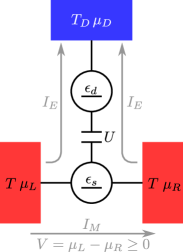
III.3 Model

The model is schematically depicted in Fig. 2. The Hamiltonian of the impurity (system and demon) reads

$$H_{\text{imp}}=\epsilon_{s}d_{s}^{\dagger}d_{s}+\epsilon_{d}d_{d}^{\dagger}d_{d}+Ud_{s}^{\dagger}d_{s}d_{d}^{\dagger}d_{d}$$ (38)

where $d_{s/d}^{\dagger}$ ($d_{s/d}$) is a fermionic creation (annihilation) operator for the system/demon dot. The Hamiltonian describes two dots with on-site energies $\epsilon_{s}$ and $\epsilon_{d}$ and Coulomb interaction $U$, which we will treat exactly with our method. Note that there are no electrons tunneling between the dots.

The non-interacting reservoirs $\nu\in\{L,R,D\}$ are modeled as free fermions as in Eq. (1) with Hamiltonian $H_{R}^{(\nu)}=\sum_{k}\epsilon_{k\nu}c^{\dagger}_{k\nu}c_{k\nu}$. The reservoirs $L$ and $R$ are tunnel-coupled to the system quantum dot via the Hamiltonian

$$H_{I}^{(\nu)}=\sum_{k}\left(t_{k\nu}d_{s}c_{k\nu}^{\dagger}+t_{k\nu}^{*}c_{k\nu}d_{s}^{\dagger}\right)~{}~{}~{}(\nu\in\{L,R\}),$$ (39)

whereas the reservoir $D$ is tunnel-coupled to the demon dot via

$$H_{I}^{(D)}=\sum_{k}\left(t_{kD}d_{d}c_{kD}^{\dagger}+t_{kD}^{*}c_{kD}d_{d}^{\dagger}\right).$$ (40)

The total Hamiltonian then reads $H_{\text{tot}}=H_{\text{imp}}+\sum_{\nu\in\{L,R,D\}}(H_{I}^{(\nu)}+H_{R}^{(\nu)})$. Within the weak coupling approach each reservoir is assumed to be well described by an equilibrium distribution according to a temperature $T_{\nu}$ and chemical potential $\mu_{\nu}$. Below, we will set for simplicity $T_{L}=T_{R}\equiv T$ and $\mu_{L}=\epsilon_{s}+V/2$ and $\mu_{R}=\epsilon_{s}-V/2$ where $V=\mu_{L}-\mu_{R}\geq 0$ denotes the bias voltage across the system.

The SD $J^{(\nu)}(\omega)$ of each reservoir $\nu$ is modeled by a Lorentzian as in Eq. (27) with coupling strength $\Gamma_{\nu}$, peak width $\Delta_{\nu}$ and resonance frequency $\omega_{0\nu}$. In the following, we will set $\Gamma_{L}=\Gamma_{R}\equiv\Gamma_{S}$ and $\Delta_{L}=\Delta_{R}\equiv\Delta_{S}$, i.e., the system is coupled with equal strength to the left and to the right reservoir and only the position of the peaks will be different.

Figure 3: A possible stochastic trajectory which becomes likely in the MD regime as explained at the end of this caption. In contrast to Fig. 2, we here sketched the transition frequencies $\epsilon_{s},\epsilon_{d},\epsilon_{s}+U$ and $\epsilon_{d}+U$ in the dots. The Fermi distribution in the baths are shown as density profiles where the darkness of the color is proportional to the occupancy of that energy. To complete the picture we also sketched the Lorentzian SDs of each reservoir whose product with the Fermi function determines the transition rates (see Appendix A). The trajectory starts with a filled dot of the demon but an empty dot of the system (1). If an electron wants to enter the system, it needs an energy $\epsilon_{s}+U$ and, although the Fermi factor is smaller for the right reservoir, this is overcompensated by the imbalance of the Lorentzian tunneling rates (2). After an electron has entered the system, it pushes the electron in the demon dot to a higher energy above the chemical potential such that it instantaneously jumps out of the dot due to requirement (44) (3). Finally, and again due to the imbalance of the Lorentizian tunneling rates, the electron in the system dot leaves to the left bath and the demon dot gets refilled (4). Overall, one electron was transfered against the bias by harnessing the correlation between the system and the demon dot and by transfering an energy amount $U$ from the hot to the cold reservoir.

III.4 Thermodynamics in the idealized limit

In the idealized picture the device is weakly coupled to three Markovian thermal reservoirs as depicted in Fig. 2. Within this approach the dynamics of the system is governed by a master equation (ME) with rates obtained from Fermi’s golden rule, see Ref. Strasberg et al. (2013) for the full rate ME. Alltogether the system works as a thermoelectric device Sánchez and Büttiker (2011); Strasberg et al. (2013). If we set $T_{D}<T$, the device is able to convert an energy current $I_{E}\equiv-I_{E}^{(D)}>0$ flowing into the reservoir $D$ into an electric current $I_{M}\equiv I_{M}^{(L)}<0$ flowing against the bias $V$ provided that the SDs $J^{(\nu)}(\omega)$ and other parameters are choosen appropriately [for a definition of energy and matter currents see Eqs. (65) and (66)]. Because the device is out of equilibrium, it produces entropy at a rate

$$\dot{\Sigma}=\beta VI_{M}+(\beta_{D}-\beta)I_{E}\geq 0.$$ (41)

It is also possible to give compact analytical expressions for $I_{M}$ and $I_{E}$ in terms of the steady state Sánchez and Büttiker (2011); Strasberg et al. (2013), but for our purposes it suffices to note the following proportionality relation:

$$I_{M}\sim\Gamma_{S}.$$ (42)

This means that the power output of the device is directly proportional to the coupling strength $\Gamma_{S}$ in the weak coupling regime and hence, it is desirable to choose $\Gamma_{S}$ as large as possible. Furthermore, we add that one can associate a second law to the local dynamics of the system only, which reads Horowitz and Esposito (2014)

$$\dot{\Sigma}_{S}=\beta VI_{M}-\beta I_{E}-\dot{{\cal{I}}}_{S}\geq 0.$$ (43)

Here, $\dot{{\cal{I}}}_{S}$ is the flow of mutual information between the system and the demon (for a precise definition see Ref. Horowitz and Esposito (2014)). Eq. (43) shows that the ability to shovel electrons against the bias, $\beta VI_{M}<0$, can be influenced by energetic ($\beta I_{E}$) as well as entropic ($\dot{{\cal{I}}}_{S}$) contributions.

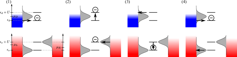
More importantly for our discussion, there is a clean limit in which the system can be viewed as an autonomous MD and in which the reduced dynamics of the system quantum dot coincides with the ideal, non-autonomous MD studied in Ref. Schaller et al. (2011). In this regime the stochastic trajectory shown in Fig. 3 becomes likely and transport against the bias possible. We will shortly review here this limit for completeness, more details can be found elsewhere Strasberg et al. (2013); Horowitz and Esposito (2014). The three different limits we need to take are the following (compare also with Sec. III.1):

1. Fast demon: First, the demon needs to be relatively fast in order to adapt quickly enough to the system state such that it is guaranteed that the correct feedback loop is applied. This is ensured by demanding that

   $$\Gamma_{D}\gg\Gamma_{S},$$ (44)

   implying that the demon is much more strongly coupled to its reservoir than the system, cf. Eq. (34). Within the formal limit $\Gamma_{D}/\Gamma_{S}\rightarrow\infty$, the demon dot can be adiabatically eliminated and a closed effective description for the system dot alone emerges. In the strict limit the flow of mutual information becomes exactly identical to $\dot{{\cal{I}}}_{S}=-\beta_{U}I_{E}$ so that the effective second law coincides with the true second law, $\dot{\Sigma}_{S}=\dot{\Sigma}$.

2. Precise demon: In order to use the demon as a detector, it should also be precise in the sense that it is as correlated as possible with the system since this increases the mutual information [compare with Eq. (32)]. Optimal results can be achieved by choosing the chemical potential of the demon such that $\epsilon_{d}=\mu_{D}-U/2$ and by requiring [cf. Eq. (35)]

   $$\beta_{D}U\gg 1.$$ (45)

   Then, in the strict limit of $\Gamma_{D}/\Gamma_{S}\rightarrow\infty$ and $\beta_{D}U\rightarrow\infty$ the demon dot is occupied if and only if the system dot is empty and vice versa implying a perfect (anti-) correlation between the system and the demon. It should be noted, however, that this strict limit also implies a diverging entropy production rate (41). Additional details concerning the use of such setups as detection devices can be found in Refs. Schaller et al. (2010); Schulenborg et al. (2014).

3. Maxwell demon: Within the fast and precise demon limit, the demon can be reliably interpreted as a detector, yet it still disturbs the energetic balances of the system at the order of $U$. Not very surpisingly, the MD limit consists of demanding that

   $$\beta V\approx 1,~{}~{}~{}\beta(V+U)\approx 1,~{}~{}~{}\frac{U}{\epsilon_{s}}\ll 1,$$ (46)

   which is in agreement with Eqs. (30) and (36) if we note that the energy current through the system is roughly proportional to $\epsilon_{S}I_{M}$ in the limit of negligible $U$. Thus, in this limit the difference in energy transfered from the right to the left reservoir (which is given by the flow of energy in the detector bath $I_{E}$) becomes immeasurably small compared to the energetic current $\epsilon_{S}I_{M}$. In this regime the term $\beta I_{E}$ becomes negligible and the second law reads

   $$\dot{\Sigma}=\dot{\Sigma}_{S}=\beta VI_{M}-\dot{{\cal{I}}}_{S}\geq 0,$$ (47)

   i.e., the ability to shovel electrons against the bias is purely entropy (or information) dominated.

The above three limits are, however, not sufficient to shovel electrons against the bias. In order to achieve this, we also need to break the left-right symmetry of the device even in the absence of any bias ($V=0$). This is most easily done by choosing different SDs $J^{(L)}(\omega)$ and $J^{(R)}(\omega)$ fulfilling $J^{(L)}(\epsilon_{s})>J^{(L)}(\epsilon_{s}+U)$ and $J^{(R)}(\epsilon_{s})<J^{(R)}(\epsilon_{s}+U)$ as depicted in Fig. 3. More specifically, we choose for our Lorentzian SDs

$$\omega_{0L}=\epsilon_{s},~{}~{}~{}\omega_{0R}=\epsilon_{s}+U.$$ (48)

The imbalance in the SDs is then quantified by

$$\frac{J^{(L)}(\epsilon_{s})}{J^{(L)}(\epsilon_{s}+U)}=\frac{J^{(R)}(\epsilon_{s}+U)}{J^{(R)}(\epsilon_{s})}=1+\frac{U^{2}}{\Delta_{S}^{2}},$$ (49)

which was previously Strasberg et al. (2013) described by the parameter $e^{\delta}$.

Furthermore, we choose to fix the following parameters for all upcoming numerical calculations: We set the on-site energies equal $\epsilon_{s}=\epsilon_{d}=\epsilon$, the inverse temperature to $\beta\epsilon=1$, and we choose a small, but finite positive bias $V=0.01\epsilon$. In addition, we set $U=0.015\epsilon$ such that it is small compared to the system energy, see Eq. (46). The SD of the demon is peaked around $\omega_{0D}=\mu_{D}=\epsilon_{d}+U/2$ and we choose $\Delta_{D}=0.01\epsilon$. The coupling strength of the demon is set to $\Gamma_{D}=100\Gamma_{S}$ ensuring that the demon is fast enough.

Thus, there are three free parameters left: (1) the variance $\Delta_{S}$ of the Lorentzian SD of the left and right reservoir controls the imbalance of the SDs [see Eq. (49)] thereby having influence on the power output and the validity of the Markov approximation; (2) the tunneling rate $\Gamma_{S}$ which controls the work output [see Eq. (42)] and (via $\Gamma_{D}=100\Gamma_{S}$) the strength of the coupling between the demon dot and its reservoir; and (3) the temperature ratio $\beta_{D}/\beta$ influencing the precision of the demon [see Eq. (45)] and thus, the correlation with the system.

Figure 4: Sketch of the geometry of the extended models studied in the text. Each circle represents a single fermionic site (“quantum dot”). The tunnel coupling is indicated by straight lines and the Coulomb interaction by a capacitor. The three reservoirs as well as the energy and electric current are also indicated as in Fig. 2.

IV Electronic Maxwell demon beyond weak coupling

In this section we report our main findings which are based on numerical comparison of the ideal (i.e., weakly coupled, Markovian and high temperature) model, see Sec. III.4, with the extended RC approach able to go beyond these limitations. We will focus on the steady state behaviour only and compare three important quantities.

First, the electric current $I_{M}$ flowing through the system dot from the left to the right reservoir. It is directly proportional to (minus) the work output of the device and is therefore an important quantifier for the overall thermodynamic performance.

Second, we look at the relative energetic imbalance $|I_{E}/I_{E}^{(L)}|$ where $I_{E}=-I_{E}^{(D)}$ denotes the energy flow into the demon reservoir and $I_{E}^{(L)}$ the energy flow from reservoir $L$ [for a definition of energy and particle currents, see Eqs. (65) and (66)]. If this quantity is large, the device works in an energy dominated regime, whereas it goes to zero in the Maxwell demon limit (46).

Third, we will evaluate the mutual information ${\cal{I}}_{S:D}$ between the system and the demon dot. It reveals key insights about the question whether the working mechanism of the device can be seen as some implicit measurement and feedback loop, which needs large correlations. Note that for our setup $0\leq{\cal{I}}_{S:D}\leq 2\ln 2$, but the maximum value is attained only for a pure and maximally entangled state. The classical limit is instead ${\cal{I}}_{S:D}^{\text{cl}}\leq\ln 2$ such that values relatively close to this limit signify already strong correlations in our noisy setup. In our numerical studies we have found that it suffices to restrict the plots of the mutual information to the interval $[0,\ln 2]$, although this does not a priori imply that there are no quantum correlations present.

IV.1 Extended models

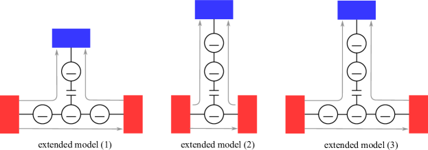
The validity of the standard ME approach as sketched in Appendix A is limited by the coupling strength to the reservoirs, the degree of non-Markovianity and the temperature of the reservoirs. In principle, all three limitations are challenged by the electronic MD model from Sec. III. We therefore compare it with three different extended models:

(1) The working mechanism of our device requires a breaking of the left-right symmetry, which was achieved by choosing different SDs $J^{(L)}(\omega)$ and $J^{(R)}(\omega)$ peaked around $\epsilon_{s}$ and $\epsilon_{s}+U$ respectively. In the ideal case, where the peaks are very narrow, the SDs act like perfect electron filters increasing the thermoelectric performance. Quite problematically, however, a strongly peaked SD is usually associated with strong non-Markovianity Zedler et al. (2009); de Vega and Alonso (2017). In order to capture the non-Markovian behaviour of the left and right reservoir, we introduce fermionic RCs $C_{l}^{(\dagger)}$ and $C_{r}^{(\dagger)}$ for the left and the right reservoir in what we call “model 1”. For the spectral densities centered at $\omega_{0,L}=\epsilon_{s}$ and $\omega_{0,R}=\epsilon_{s}+U$, the resulting redefined impurity Hamiltonian reads

$$\begin{split}\tilde{H}_{\text{imp}}^{(1)}=&~{}H_{\text{imp}}+\epsilon_{s}C_{l}^{\dagger}C_{l}+(\epsilon_{s}+U)C_{r}^{\dagger}C_{r}\\ &+\sqrt{\frac{\Gamma_{S}\Delta_{S}}{2}}\left(C_{l}^{\dagger}d_{s}+d_{s}^{\dagger}C_{l}+C_{r}^{\dagger}d_{s}+d_{s}^{\dagger}C_{r}\right)\end{split}\,,$$ (50)

and the coupling to the residual left and right reservoir is described by a flat SD $J_{1}^{(\nu)}(\omega)=2\Delta_{S}$, $\nu\in\{L,R\}$. A sketch of the setup is shown in Fig. 4. We remark that the inclusion of additonal quantum dots to model peaked SDs acting as energy filtes has been used elsewhere, too Sánchez and Büttiker (2011); Sánchez et al. (2008, 2017).

(2) Putting the problem of non-Markovianity aside, the most pressing problem is that the demon dot must be relatively strongly coupled to a low temperature heat reservoir. This problem becomes more pronounced if we want to enhance the power output by increasing $\Gamma_{S}$. Model (2) therefore introduces a fermionic RC $C_{d}^{(\dagger)}$ for the demon bath in order to study those effects. When we use $\omega_{0,D}=\epsilon_{d}+U/2$, the resulting redefined impurity Hamiltonian reads

$$\begin{split}\tilde{H}_{\text{imp}}^{(2)}=&~{}H_{\text{imp}}+\left(\epsilon_{d}+\frac{U}{2}\right)C_{d}^{\dagger}C_{d}\\ &+\sqrt{\frac{\Gamma_{D}\Delta_{D}}{2}}(C_{d}^{\dagger}d_{d}+d_{d}^{\dagger}C_{d})\end{split}$$ (51)

and the coupling to the residual demon reservoir is described by a flat SD $J_{1}^{(D)}(\omega)=2\Delta_{D}$. A sketch of the setup is again shown in Fig. 4.

(3) In order to capture both problems, model 3 finally uses a fermionic RC for all reservoirs, see Fig. 4. Within our framework this will provide the ultimate test for the simplied model from Sec. III.4. The redefined Hamiltonian is given by the sum of Eq. (50) and (51) without counting $H_{\text{imp}}$ twice,

$$\tilde{H}_{\text{imp}}^{(3)}=\tilde{H}_{\text{imp}}^{(1)}+\tilde{H}_{\text{imp}}^{(2)}-H_{\text{imp}}.$$ (52)

The SDs of the residual reservoirs $L,R$ and $D$ are given by $2\Delta_{S},2\Delta_{S}$ and $2\Delta_{D}$, respectively.

Figure 5: Plot of the dimensionless quantities $I_{M}/\Gamma_{S}$ (top), $I_{E}/I_{E}^{(L)}$ (bottom) and ${\cal{I}}_{S:D}$ (inset) versus the dimensionless sharpness of the peak of the left and right SDs $\Delta_{S}/\epsilon_{s}$ (note the logarithmic scale). Results using the extended model (1) are shown with a solid line, the dotted red line refers to the DQDMD description from Sec. III.4. The shaded grey area indicates the region where the DQDMD treatment and the MD interpretation is valid. To remain in the strict weak coupling regime, we chose $\Gamma_{S}=10^{-5}\epsilon_{s}$. Furthermore, $\beta_{D}/\beta=300$.

IV.2 Numerical results

In what follows, we will compare the results of our extended models with the original MD treatment exposed in Sec. III.4. We will refer to the latter as double quantum dot Maxwell demon (DQDMD) treatment and use red, dashed lines in the plots. The regime where the simple double quantum dot treatment and the MD interpretation are valid are shaded in grey in the plots.

IV.2.1 RCs for the system reservoirs

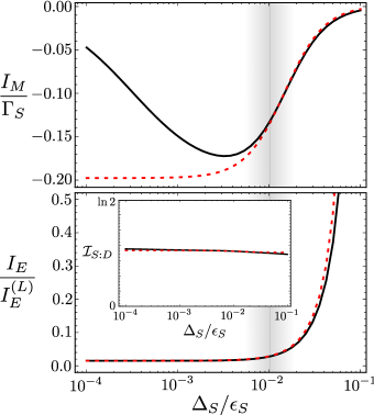
We start with the extended model (1) to answer the question how narrowly peaked can we choose the SDs $J^{(\nu)}(\omega)$ before the Markovian description from Sec. III.4 breaks down? The answer is shown in Fig. 5. It clearly shows that there is an optimum value for the sharpness of the peak, which can be found by maximizing the power output $-VI_{M}$ while still retaining a valid Markovian description.

For $\Delta_{S}\rightarrow 0$ the RC description indeed predicts $I_{M}\rightarrow 0$ because the coupling to the residual baths is directly proportional to $\Delta_{S}$. It is worth to emphasize that the naive ME treatment of Sec. III.4 predicts a monotonically increasing power output in the limit $\Delta_{S}\rightarrow 0$ in strong contrast to the actual behaviour. We conclude that one has to be very careful if one chooses strongly preaked SDs (sometimes called “spectral filters”) to increase the power output of a thermodynamic device.

In the opposite limit, $\Delta_{S}\rightarrow\infty$, the engine also breaks down because the SDs become essentially flat and the left-right symmetry remains unbroken. Note that the amount of mutual information between the system and the demon is almost unaffected by the shape of the SD as expected.

Although the simple DQDMD description becomes inaccurate below a certain critical threshold $\Delta_{S}^{*}/\epsilon_{s}\approx 0.01$, the plot also shows (shaded grey region) that a Markovian description is valid even if the SD is not completely flat but slightly structured [at the critical value, the imbalance (49) is for the choosen numerical parameters roughly $1.18$]. Finally, we note that the regime, where the Markovian description is valid while at the same time the energetic imbalance is very small (less than $5\%$), is restricted to a very narrow window around $\Delta^{*}_{S}/\epsilon_{s}$ demonstrating the careful finetuning needed to ensure a working autonomous MD.

Figure 6: Plot of our three relevant quantities versus the dimensionless coupling strength $\Gamma_{S}$ of the system (note the logarithmic scale again) for the extended model (2) (solid line) and the DQDMD treatment (dotted red line). The shaded grey area indicates the region where the DQDMD treatment and the MD interpretation is valid. Parameters as in Fig. 5 with $\Delta_{S}/\epsilon_{s}=0.01$.

Figure 7: Plot of our three relevant quantities versus the dimensionless inverse temperature $\beta_{D}/\beta$ of the demon reservoir (in logarithmic scale) for $\Gamma_{S}=10^{-4}\epsilon_{s}$ (main plots) and $\Gamma_{S}=10^{-5}\epsilon_{s}$ (insets). The rest is as in Fig. 6.

IV.2.2 RC for the demon reservoir

Numerical results associated to model (2) concerning the question what happens to the demon in the strong coupling and low temperature regime are shown in Figs. 6 and 7.

Figure 8: Repetition of the plots shown before for the extended model (3). In all plots we chose $\Gamma_{S}=10^{-5}\epsilon_{s}$, $\Delta_{S}=0.01\epsilon_{s}$ and $\beta_{D}/\beta=300$ unless that parameter is varied in the respective plot. The grey shaded area indicates the region, in which the ideal MD interpretation holds.

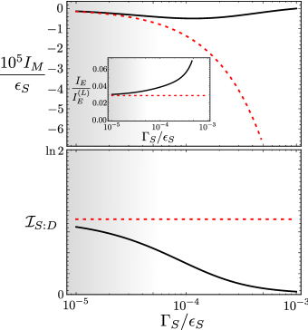
First, Fig. 6 shows our three relevant quantities as a function of $\Gamma_{S}$, which (in the weak coupling regime) is directly proportional to the power output of the device [Eq. (42)] and influences the demon coupling strength via our choice $\Gamma_{D}=100\Gamma_{S}$. Numerical parameters are the same as in Fig. 5 with the choice $\Delta_{S}=\Delta_{S}^{*}=0.01\epsilon_{s}$. As expected, the plot of the electric current $I_{M}$ demonstrates that the DQDMD treatment is only valid for very small coupling strength $\Gamma_{S}<10^{-4}\epsilon_{s}$ (shaded grey region), beyond that the demon fails to work. Also the plot of the relative energy imbalance $I_{E}/I_{E}^{(L)}$ shows that we are leaving the MD regime of negligible energy consumption for larger $\Gamma_{S}$ because more transport channels are opening up. More interestingly, however, is the plot of the mutual information ${\cal{I}}_{S:D}$, which reveals the physical reason why the demon fails. As explained in Sec. III, the working mechanism is based on a strong correlation between the demon and the system due to the Coulomb interaction and a careful tuning of the demon’s reservoir. But for stronger coupling the electron in the demon dot gets more and more correlated with its reservoir than with the system, i.e., it becomes more and more delocalized. The only way to counter balance this behaviour is by increasing the Coulomb interaction $U$, but this increases the energy imbalance pushing us away from the MD regime. This is the ultimate reason why the MD is limited to the weak coupling situation and thus, due to the required time-scale separation $\Gamma_{D}\gg\Gamma_{S}$, to very low power output.

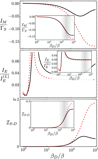
To complement the analysis, Fig. 7 shows the same quantities for varying inverse temperature $\beta_{D}$ for relatively strong coupling strength $\Gamma_{S}=10^{-4}\epsilon_{s}$ and, shown as insets, for $\Gamma_{S}=10^{-5}\epsilon_{s}$, which was used in Fig. 5. As expected, for larger $\Gamma_{S}$ we see stronger deviations from the ideal values confirming our previous observation. In addition, Fig. 7 demonstrates two more important features. First, the device works better for lower temperatures because the formation of correlations is hindered if the demon is subjected to more thermal noise. Second, this figure also shows that a DQDMD description is usually only valid at high temperatures, whereas more sophisticated methods are needed for lower temperatures. We stress once more that, though the RC method allows to treat lower temperatures, its validity also does not extend down to zero temperature $T_{D}\rightarrow 0$.

IV.2.3 RCs for all reservoirs

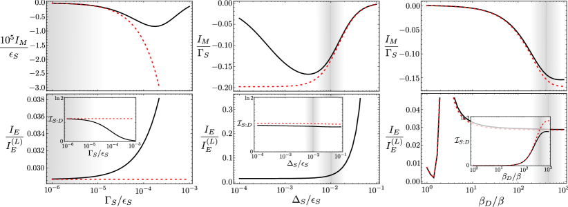
Finally, numerical results using model (3) are shown in Fig. 8. It is our most accurate analysis and combines model (1) and (2) and the plots demonstrate that the results, which we have drawn above in a separate analysis, hold true also in the complete picture. Furthermore, although the simple DQDMD picture from Sec. III.4 fails for most parameters as expected, it also agrees well if we pay careful attention to its range of validity. Thus, the analysis of the ideal MD Strasberg et al. (2013), despite the various limits involved, remains qualitatively and quantitatively true for a narrow parameter window.

V Summary

In this article we have developed the theory of fermionic RCs, which provides a tool to extend the range of validity of the usual ME, especially for very structured, i.e., strongly non-Markovian, SDs. The benefit of our approach is that the ME approach still allows to treat interactions in the system exactly, it can be straightforwardly applied to nonequilibrium situations and has a transparent thermodynamic interpretation. One drawback of the method is that not every initial SD can be mapped to an effectively weakly coupled and Markovian situation such that the application of the ME has to be justified on a case-by-case study. Another drawback comes from the use of a ME itself, which becomes invalid at very low temperatures. Nevertheless, we believe that the fermionic RC mapping has the potential to find widespread application in quantum transport as a simple and transparent tool to treat structured SDs.

As a particular application we then considered a thermoelectric device, which can be interpreted as an autonomous MD for a specific range of parameters. Previous analyses in the field of information thermodynamics were done in the idealized weak coupling and Markovian regime, an exception being Ref. Walldorf et al. (2017). As we have argued in Sec. III.1 and as Ref. Strasberg et al. (2013) explicitly shows, MD lives in a parameter regime where the use of these idealized assumptions becomes increasingly questionable. We here addressed for the first time systematically the question of what happens to the performance of an autonomous MD if we relax the weak coupling and Markovian assumption (also see Ref. Schaller et al. (2017) for the study of a non-autonomous MD in the strong coupling regime).

Our numerical results clearly convey two messages: First, we have proven that it is indeed possible to reach the idealized MD regime, even if one uses a more sophisticated method, which is able to take into account strong coupling and non-Markovian effects. Thus, MD is not a mere hypothetical being, but can be found in actual physical systems. On the other hand, our article also indicates that the possible parameter regime of an ideal MD is very narrow and necessarily limited to low power output. It therefore still remains a challenge to find out to what extend MD will play a role in actual, practically useful devices, where already the use of a model Hamiltonian of the form (38) amounts to a strong assumption as it neglects, e.g., spin and vibrational degrees of freedom as well as multiple charges on a single quantum dot.

Acknowledgements. Important initial discussions with Tobias Brandes on the fate of Maxwell’s demon in the strong-coupling and low temperature regime have led to these investigations. GS acknowledges financial support by the DFG (SCHA 1646/3-1, SFB 910, and GRK 1558), TLS acknowledges support from the National Research Fund Luxembourg (ATTRACT 7556175), and PS and ME by the European Research Council project NanoThermo (ERC-2015-CoG Agreement No. 681456). GS and PS furthermore acknowledge support of the WE-Heraeus foundation for supporting the 640 WE-Heraeus seminar.

Appendix A Derivation of the master equation

In this appendix we briefly state the essential steps to derive the quantum ME used in the main text. We start by focusing on an impurity (also often called the “system”) coupled to a single reservoir with Hamiltonian $H_{\text{tot}}=H_{\text{imp}}+H_{I}+H_{R}$. Because within the weak coupling approach there is no direct influence between the different reservoirs, we can simply add the contributions of them at the end. More detailed derivations of MEs can be found elsewhere Breuer and Petruccione (2002); Schaller (2014); de Vega and Alonso (2017); Esposito et al. (2009). Note that $H_{\text{imp}}$, $H_{I}$ and $H_{R}$ are arbitrary and left unspecified here. For the MEs used in Sec. IV one would indeed need to replace $H_{\text{imp}}$ by $\tilde{H}_{\text{imp}}$.

Our starting point is the second order Liouville-von Neumann equation in the interaction picture after performing the Markovian approximation

$$\begin{split}d_{t}\tilde{\rho}(t)=-\int_{0}^{\infty}d\tau&\mbox{tr}_{B}\left\{\tilde{H}_{I}(t)\tilde{H}_{I}(t-\tau)\tilde{\rho}(t)R_{0}\right.\\ &\left.-\tilde{H}_{I}(t)\tilde{\rho}(t)R_{0}\tilde{H}_{I}(t-\tau)+h.c.\right\}\end{split}$$ (53)

where $\tilde{A}(t)\equiv e^{i(H_{\text{imp}}+H_{R})t}Ae^{-i(H_{\text{imp}}+H_{R})t}$ denotes operators in the interaction picture and $R_{0}=e^{-\beta(H_{R}-\mu N_{R})}/Z$ describes the equilibrium density operator of the reservoir with $N_{R}$ being the particle number operator of the reservoir.

For our purposes it suffices to consider an interaction Hamiltonian of the form

$$H_{I}=d\sum_{k}t_{k}c_{k}^{\dagger}+\sum_{k}t_{k}^{*}c_{k}d^{\dagger}$$ (54)

where $d$ is an arbitrary fermionic system operator. We denote the eigensystem and transition frequencies of $H_{\text{imp}}$ as

$$H_{\text{imp}}=\sum_{k}E_{k}|k{\rangle\langle}k|,~{}~{}~{}\omega_{kl}\equiv E_{k}-E_{l}$$ (55)

such that we can write the system coupling operator in the interaction picture as

$$\tilde{d}(t)=\sum_{k,l}e^{i\omega_{kl}t}d_{kl}|k{\rangle\langle}l|,~{}~{}~{}d_{kl}\equiv\langle k|d|l\rangle.$$ (56)

Then, after introducing the SD $J(\omega)=2\pi\sum_{k}|t_{k}|^{2}\delta(\omega-\epsilon_{k})$ of the bath and after moving out of the interaction picture, we obtain terms like

$$e^{-iH_{\text{imp}}t}\mbox{tr}_{B}\{\tilde{H}_{I}(t)\tilde{H}_{I}(t-\tau)\tilde{\rho}(t)R_{0}\}e^{iH_{\text{imp}}t}$$

$$~{}~{}~{}=\int_{-\infty}^{\infty}d\omega\frac{J(\omega)}{2\pi}\sum_{k,l}\left\{e^{i(\omega+\omega_{kl})\tau}f(\omega)dd^{*}_{kl}|l{\rangle\langle}k|\rho(t)+e^{-i(\omega+\omega_{kl})\tau}[1-f(\omega)]d^{\dagger}d_{kl}|k{\rangle\langle}l|\rho(t)\right\},$$ (57)

$$e^{-iH_{\text{imp}}t}\mbox{tr}_{B}\{\tilde{H}_{I}(t)\tilde{\rho}(t)R_{0}\tilde{H}_{I}(t-\tau)\}e^{iH_{\text{imp}}t}$$

$$~{}~{}~{}=\int_{-\infty}^{\infty}d\omega\frac{J(\omega)}{2\pi}\sum_{k,l}\left\{e^{i(\omega+\omega_{kl})\tau}[1-f(\omega)]d\rho(t)d^{*}_{kl}|l{\rangle\langle}k|+e^{-i(\omega+\omega_{kl})\tau}f(\omega)d^{\dagger}\rho(t)d_{kl}|k{\rangle\langle}l|\right\}$$ (58)

and their Hermitian conjugate. Here, $f(\epsilon_{k})=\mbox{tr}_{B}\{c_{k}^{\dagger}c_{k}R_{0}\}=[e^{\beta(\epsilon_{k}-\mu)}+1]^{-1}$ denotes the Fermi distribution.

To evaluate the integral over $\tau$, we then use

$$\int_{0}^{\infty}d\tau e^{\pm i\omega\tau}=\pi\delta(\omega)\pm i{\cal{P}}\frac{1}{\omega}$$ (59)

and neglect the imaginary principal value part in the following (cf. Appendix B). After this step the full ME can be written as

$$\begin{split}d_{t}\rho(t)=&-i[H_{\text{imp}},\rho(t)]+[\chi^{\dagger}\rho(t),d]+[d^{\dagger},\rho(t)\chi]\\ &+[\theta\rho(t),d^{\dagger}]+[d,\rho(t)\theta^{\dagger}].\end{split}$$ (60)

where we introduced the operators

$$\chi \equiv\sum_{k,l}\frac{J(\omega_{lk})}{2}f(\omega_{lk})d_{kl}|k{\rangle\langle}l|,$$ (61)

$$\theta \equiv\sum_{k,l}\frac{J(\omega_{lk})}{2}[1-f(\omega_{lk})]d_{kl}|k{\rangle\langle}l|.$$ (62)

The ME (60) is ready for numerical implementation. Note that we did not perform the commonly employed secular approximation, which guarantees a Lindblad form of the generator Breuer and Petruccione (2002); Schaller (2014); de Vega and Alonso (2017); Esposito et al. (2009), but often predicts unphysical results especially for more complex systems, see also Appendix B.

If we include coupling to multiple baths characterized by a distinct chemical potential or temperature, we can simply add up the contribution of each bath separately to the ME. The result is then

$$d_{t}\rho(t)=-i[H_{\text{imp}},\rho(t)]+\sum_{\nu}{\cal{L}}_{\nu}\rho(t)$$ (63)

with the dissipator

$${\cal{L}}_{\nu}\rho\equiv[\chi_{\nu}^{\dagger}\rho,d_{\nu}]+[d_{\nu}^{\dagger},\rho\chi_{\nu}]+[\theta_{\nu}\rho,d_{\nu}^{\dagger}]+[d_{\nu},\rho\theta_{\nu}^{\dagger}].$$ (64)

The energy and particle currents into bath $\nu$ are then given by

$$I_{E}^{(\nu)} =\mbox{tr}\{H_{\text{imp}}{\cal{L}}_{\nu}\rho(t)\},$$ (65)

$$I_{M}^{(\nu)} =\mbox{tr}\{N_{\text{imp}}{\cal{L}}_{\nu}\rho(t)\},$$ (66)

where $N_{\text{imp}}$ is the particle number operator of the impurity.

Appendix B Example and benchmark: Single electron transistor

Figure 9: Plot of the matter current over the dimensionless coupling strength $\beta\Gamma$ in logarithmic scale computed using different methods: the naive rate equation approach (thin dotted green), the exact solution (thick red), and the RC approach based on different levels of approximation for the ME: The Born-Markov treatment of Eq. (60) including the Lamb shift terms from Eq. (59) (RC+BM, thin solid dark blue curve), Eq. (60) neglecting the Lamb shift (RC+BM-LS, dashed bold light blue curve), and Eq. (60) with an additional secular approximation (BMS, thin dash-dotted solid black). Parameters are $\Delta=0.1\epsilon,\omega_{0}=\epsilon,\beta\epsilon=1$ and $\mu_{L}=\epsilon=-\mu_{R}$.

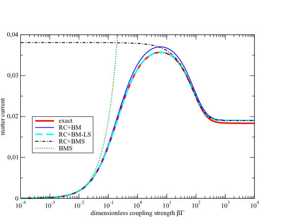
To benchmark our approach we consider the possibly simplest fermionic transport setup usually called a single electron transistor (SET): a spinless quantum dot with on-site energy $\epsilon$ coupled to two fermionic baths $\nu\in\{L,R\}$. In this case we have $H_{\text{imp}}=\epsilon d^{\dagger}d$ and we model the contact to the baths again by a Lorentzian of the form (27), which we assume to be the same for the left and right reservoir.

Figure 10: Plot of the energy current instead of the matter current with the same parameters as in Fig. 10.

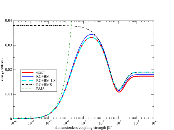
Figs. 9 and 10 now compare the energy and particle current through the SET using three different methods. The first (dotted green) is based on a standard rate equation for the probability to find the quantum dot empty or filled (i.e., the ME from Appendix A applied to $H_{\text{imp}}=\epsilon d^{\dagger}d$). The second method makes use of a single RC mapping individually applied to each reservoir and yields the Hamiltonian

$$\tilde{H}_{\text{imp}}=H_{\text{imp}}+\sum_{\nu}\left(\lambda_{0}dC_{1\nu}^{\dagger}+\lambda_{0}^{*}C_{1\nu}d^{\dagger}+E_{1}C_{1\nu}^{\dagger}C_{1\nu}\right),$$ (67)

which now consists of three serially coupled quantum dots. The second method then treats the residual baths as weakly coupled and Markovian by using the ME treatment from Appendix A. In addition, it allows for different perturbative treatments by either including (solid dark-blue line) or neglecting (dashed light-blue line) Lamb shift terms or by performing an additional secular approximation on top (dash-dotted black line). Finally, the model also admits an exact solution for the matter and energy current which reads (solid red line; compare with, e.g., Ref. Topp et al. (2015))

$$I_{M} =\int_{-\infty}^{\infty}\frac{2d\omega}{\pi}\frac{J_{L}(\omega)J_{R}(\omega)[f_{L}(\omega)-f_{R}(\omega)]}{[J_{L}(\omega)+J_{R}(\omega)]^{2}+4[\omega-\epsilon-\Sigma(\omega)]^{2}},$$

$$I_{E} =\int_{-\infty}^{\infty}\frac{2d\omega}{\pi}\frac{\omega J_{L}(\omega)J_{R}(\omega)[f_{L}(\omega)-f_{R}(\omega)]}{[J_{L}(\omega)+J_{R}(\omega)]^{2}+4[\omega-\epsilon-\Sigma(\omega)]^{2}}.$$

Here, $\Sigma=\Sigma_{L}+\Sigma_{R}$ denotes the Lamb shift

$$\begin{split}\Sigma_{\nu}(\omega)&\equiv{\cal{P}}\int\frac{d\omega^{\prime}}{2\pi}\frac{J_{\nu}(\omega^{\prime})}{\omega-\omega^{\prime}}\\ &=\frac{\Gamma\Delta(\omega-\omega_{0})}{2[(\omega-\omega_{0})^{2}+\Delta^{2}]}=\frac{\omega-\omega_{0}}{2\Delta}J_{\nu}(\omega).\end{split}$$ (68)

As we can see, the RC method based on the ME (60) (i.e., without secular approximation) gives an excellent agreement with the exact result for a wide parameter regime. Generally, we see that over all coupling strengths, including or neglecting the Lamb shift has little effect. For intermediate coupling strengths, including the Lamb shift terms is even reducing the agreement with the exact solution, whereas for the ultrastrong coupling regime it is improving the agreement, as is particularly visible in the energy current. More importantly, however, we see that the often employed secular approximation fails completely in the weak to intermediate parameter regimes. These reasons justify the use of the ME we derived in Appendix A.

It is nevertheless important to remark that the RC method is also limited. First of all, in order to justify using a weak coupling ME for $\tilde{H}_{\text{imp}}$, the width $\Delta$ of the Lorentzian must be small enough because it is directly proportional to the coupling strength of the RC with the residual bath. Second, even for small $\Delta$ our approach is still based on the use of a ME invalidating our results for very low temperature. For instance, the differential conductance of the SET $\lim_{V\rightarrow 0}\frac{dI_{M}}{dV}$ computed with the RC method completely fails to reproduce the exact results for $T\rightarrow 0$ (not shown here for brevity).

References

- Breuer and Petruccione (2002) H.-P. Breuer and F. Petruccione, The Theory of Open Quantum Systems (Oxford University Press, Oxford, 2002).
- Schaller (2014) G. Schaller, Open Quantum Systems Far from Equilibrium (Lect. Notes Phys., Springer, Cham, 2014).
- de Vega and Alonso (2017) I. de Vega and D. Alonso, “Dynamics of non-Markovian open quantum systems,” Rev. Mod. Phys. 89, 015001 (2017).
- Stefanucci and van Leeuwen (2013) G. Stefanucci and R. van Leeuwen, Nonequilibrium many-body theory of quantum systems: A modern Introduction (Cambridge University Press, New York, 2013).
- Bulla et al. (2008) R. Bulla, T. A. Costi, and T. Pruschke, “Numerical renormalization group method for quantum impurity systems,” Rev. Mod. Phys. 80, 395–450 (2008).
- Garg et al. (1985) A. Garg, J. N. Onuchic, and V. Ambegaokar, “Effect of friction on electron transfer in biomolecules,” J. Chem. Phys. 83, 4491 (1985).
- Jean et al. (1992) J. M. Jean, R. A. Friesner, and G. R. Fleming, “Application of a multilevel Redfield theory to electron transfer in condensed phases,” J. Chem. Phys. 96, 5827–5842 (1992).
- May et al. (1993) V. May, O Kühn, and M. Schreiber, “Density matrix description of ultrafast dissipative wave packet dynamics,” J. Phys. Chem. 97, 12591 (1993).
- Pollard and Friesner (1994) W. T. Pollard and R. A. Friesner, “Solution of the Redfield equation for the dissipative quantum dynamics of multilevel systems,” J. Chem. Phys. 100, 5054–5065 (1994).
- Wolfseder and Domcke (1996) B. Wolfseder and W. Domcke, “Intramolecular electron-transfer dynamics in the inverted regime: quantum mechanical multi-mode model including dissipation,” Chem. Phys. Lett. 259, 113 (1996).
- Wolfseder et al. (1998) B. Wolfseder, L. Seidner, G. Stock, W. Domcke, M. Seel, S. Engleitner, and W. Zinth, “Vibrational coherence in ultrafast electron-transfer dynamics of oxazine 1 in n,n-dimethylaniline: simulation of a femtosecond pump-probe experiment,” Chem. Phys. 233, 323 (1998).
- Hartmann et al. (2000) L. Hartmann, I. Goychuk, and P. Hänggi, “Controlling electron transfer in strong time-dependent fields: Theory beyond the golden rule approximation,” J. Chem. Phys. 113, 11159–11175 (2000).
- Thoss et al. (2001) M. Thoss, H. Wand, and W. H. Miller, “Self-consistent hybrid approach for complex systems: Application to the spin-boson model with debye spectral density,” J. Chem. Phys. 115, 2991–3005 (2001).
- Cederbaum et al. (2005) L. S. Cederbaum, Etienne E. Gindensperger, and I. Burghardt, “Short-time dynamics through conical intersections in macrosystems,” Phys. Rev. Lett. 94, 113003 (2005).
- Hughes et al. (2009a) K. H. Hughes, C. D. Christ, and I. Burghardt, “Effective-mode representation of non-Markovian dynamics: A hierarchical approximation of the spectral density. I. Application to single surface dynamics,” The Journal of Chemical Physics 131, 024109 (2009a).
- Hughes et al. (2009b) K. H. Hughes, C. D. Christ, and I. Burghardt, “Effective-mode representation of non-Markovian dynamics: A hierarchical approximation of the spectral density. II. Application to environment-induced nonadiabatic dynamics,” The Journal of Chemical Physics 131, 124108 (2009b).
- Martinazzo et al. (2011a) R. Martinazzo, B. Vacchini, K. H. Hughes, and I. Burghardt, “Communication: Universal Markovian reduction of Brownian particle dynamics,” J. Chem. Phys. 134, 011101 (2011a).
- Martinazzo et al. (2011b) R. Martinazzo, K. H. Hughes, and I. Burghardt, “Unraveling a Brownian particle’s memory with effective mode chains,” Phys. Rev. E 84, 030102 (2011b).
- Iles-Smith et al. (2014) J. Iles-Smith, N. Lambert, and A. Nazir, “Environmental dynamics, correlations and the emergence of noncanonical equilibrium states in open quantum systems,” Phys. Rev. A 90, 032114 (2014).
- Huh et al. (2014) J. Huh, S. Mostame, T. Fujita, M.-H. Yung, and A. Aspuru-Guzik, “Linear-algabraic bath transformation for simulating complex open quantum systems,” New J. Phys. 16, 123008 (2014).
- Bonfanti et al. (2015) M. Bonfanti, K. H. Hughes, I. Burghardt, and R. Martinazzo, “Vibrational relaxation and decoherence in structured environments: a numerical investigation,” Ann. Phys. 00, 1–14 (2015).
- Iles-Smith et al. (2016) J. Iles-Smith, A. G. Dijkstra, N. Lambert, and A. Nazir, “Energy transfer in structured and unstructured environments: master equations beyond the Born-Markov approximations,” J. Chem. Phys. 144, 044110 (2016).
- Prior et al. (2010) J. Prior, A. W. Chin, S. F. Huelga, and M. B. Plenio, “Efficient simulation of strong system-environment interactions,” Phys. Rev. Lett. 105, 050404 (2010).
- Chin et al. (2010) A. W. Chin, Á. Rivas, S. F. Huelga, and M. B. Plenio, “Exact mapping between system-reservoir quantum models and semi-infinite discrete chains using orthogonal polynomials,” J. Math. Phys. 51, 092109 (2010).
- Woods et al. (2014) M. P. Woods, R. Groux, A. W. Chin, S. F. Huelga, and M. B. Plenio, “Mappings of open quantum systems onto chain representations and Markovian embeddings,” J. Math. Phys. 55, 032101 (2014).
- Woods et al. (2015) M. P. Woods, M. Cramer, and M. B. Plenio, “Simulating bosonic baths with error bars,” Phys. Rev. Lett. 115, 130401 (2015).
- Woods and Plenio (2016) M. P. Woods and M. B. Plenio, “Dynamical error bounds for continuum discretisation via Gauss quadrature rules – A Lieb-Robinson bound approach,” J. Math. Phys. 57, 022105 (2016).
- Rosenbach et al. (2016) R. Rosenbach, J. Cerrillo, S. F Huelga, J. Cao, and M. B Plenio, “Efficient simulation of non-Markovian system-environment interaction,” New Journal of Physics 18, 023035 (2016).
- Esposito et al. (2010) M. Esposito, K. Lindenberg, and C. Van den Broeck, “Entropy production as correlation between system and reservoir,” New J. Phys. 12, 013013 (2010).
- Esposito et al. (2015a) M. Esposito, M. A. Ochoa, and M. Galperin, “Quantum thermodynamics: A nonequilibrium Green’s function approach,” Phys. Rev. Lett. 114, 080602 (2015a).
- Esposito et al. (2015b) M. Esposito, M. A. Ochoa, and M. Galperin, “Nature of heat in strongly coupled open quantum systems,” Phys. Rev. B 92, 235440 (2015b).
- Bruch et al. (2016) A. Bruch, M. Thomas, S. V. Kusminskiy, F. von Oppen, and A. Nitzan, “Quantum thermodynamics of the driven resonant level model,” Phys. Rev. B 93, 115318 (2016).
- Seifert (2016) U. Seifert, “First and second law of thermodynamics at strong coupling,” Phys. Rev. Lett. 116, 020601 (2016).
- Strasberg et al. (2016) P. Strasberg, G. Schaller, N. Lambert, and T. Brandes, “Nonequilibrium thermodynamics in the strong coupling and non-Markovian regime based on a reaction coordinate mapping,” New. J. Phys. 18, 073007 (2016).
- Talkner and Hänggi (2016) P. Talkner and P. Hänggi, “Open system trajectories specify fluctuating work but not heat,” Phys. Rev. E 94, 022143 (2016).
- Kato and Tanimura (2016) A. Kato and Y. Tanimura, “Quantum heat current under non-perturbative and non-Markovian conditions: Applications to heat machines,” J. Chem. Phys. 145, 224105 (2016).
- Cerrillo et al. (2016) J. Cerrillo, M. Buser, and T. Brandes, “Nonequilibrium quantum transport coefficients and transient dynamics of full counting statistics in the strong-coupling and non-Markovian regimes,” Phys. Rev. B 94, 214308 (2016).
- Whitney (2016) R. S. Whitney, “Non-Markovian quantum thermodynamics: second law and fluctuation theorems,” arXiv: 1611.00670 (2016).
- Newman et al. (2017) D. Newman, F. Mintert, and A. Nazir, “Performance of a quantum heat engine at strong reservoir coupling,” Phys. Rev. E 95, 032139 (2017).
- Jarzynski (2017) C. Jarzynski, “Stochastic and macroscopic thermodynamics of strongly coupled systems,” Phys. Rev. X 7, 011008 (2017).
- Miller and Anders (2017) H. J. D. Miller and J. Anders, “Entropy production and time asymmetry in the presence of strong interactions,” Phys. Rev. E 95, 062123 (2017).
- Strasberg and Esposito (2017) P. Strasberg and M. Esposito, “Stochastic thermodynamics in the strong coupling regime: An unambiguous approach based on coarse graining,” Phys. Rev. E 95, 062101 (2017).
- Perarnau-Llobet et al. (2017) M. Perarnau-Llobet, H. Wilming, A. Riera, R. Gallego, and J. Eisert, “Fundamental corrections to work and power in the strong coupling regime,” arXiv: 1704.05864 (2017).
- Mu et al. (2017) A. Mu, B. K. Agarwalla, G. Schaller, and D. Segal, “Qubit absorption refrigerator at strong coupling,” New J. Phys. 19, 123034 (2017).
- Haughian et al. (2018) P. Haughian, M. Esposito, and T. L. Schmidt, “Quantum thermodynamics of the resonant-level model with driven system-bath coupling,” Phys. Rev. B 97, 085435 (2018).
- Restrepo et al. (2017) S. Restrepo, J. Cerrillo, P. Strasberg, and G. Schaller, “From quantum heat engines to laser cooling: Floquet theory beyond the Born-Markov approximation,” arXiv: 1712.07032 (2017).
- Sánchez and Jordan (2015) R. Sánchez and A. N. Jordan, “Thermoelectric energy harvesting with quantum dots,” Nanotechnology 26, 032001 (2015).
- Benenti et al. (2017) G. Benenti, G. Casati, K. Saito, and R. S. Whitney, “Fundamental aspects of steady-state conversion of heat to work at the nanoscale,” Phys. Rep. 694, 1–124 (2017).
- Sánchez and Büttiker (2011) Rafael Sánchez and Markus Büttiker, “Optimal energy quanta to current conversion,” Phys. Rev. B 83, 085428 (2011).
- Strasberg et al. (2013) P. Strasberg, G. Schaller, T. Brandes, and M. Esposito, “Thermodynamics of a physical model implementing a maxwell demon,” Phys. Rev. Lett. 110, 040601 (2013).
- Hartmann et al. (2015) F. Hartmann, P. Pfeffer, S. Höfling, M. Kamp, and L. Worschech, “Voltage fluctuation to current converter with Coulomb-coupled quantum dots,” Phys. Rev. Lett. 114, 146805 (2015).
- Thierschmann et al. (2015) H. Thierschmann, R. Sánchez, B. Sothmann, F. Arnold, C. Heyn, W. Hansen, H. Buhmann, and L. W. Molenkamp, “Three-terminal energy harvester with coupled quantum dots,” Nat. Nanotechnol. 10, 854–858 (2015).
- Horowitz and Esposito (2014) J. M. Horowitz and M. Esposito, “Thermodynamics with continuous information flow,” Phys. Rev. X 4, 031015 (2014).
- Kutvonen et al. (2015) A. Kutvonen, J. Koski, and T. Ala-Nissilä, “Thermodynamics and efficiency of an autonomous on-chip Maxwell’s demon,” Sci. Rep. 6, 21126 (2015).
- Koski et al. (2015) J. V. Koski, A. Kutvonen, I. M. Khaymovich, T. Ala-Nissila, and J. P. Pekola, “On-chip Maxwell’s demon as an information-powered refrigerator,” Phys. Rev. Lett. 115, 260602 (2015).
- Walldorf et al. (2017) N. Walldorf, A.-P. Jauho, and K. Kaasbjerg, “Thermoelectrics in Coulomb-coupled quantum dots: Cotunneling and energy-dependent lead couplings,” Phys. Rev. B 96, 115415 (2017).
- Schaller et al. (2017) G. Schaller, J. Cerrillo, G. Engelhardt, and P. Strasberg, “An electronic Maxwell demon in the coherent strong-coupling regime,” arXiv: 1711.00706 (2017).
- Elattari and Gurvitz (2000) B. Elattari and S.A. Gurvitz, “Influence of measurement on the lifetime and the linewidth of unstable systems,” Phys. Rev. A 62, 032102 (2000).
- Esposito et al. (2009) M. Esposito, U. Harbola, and S. Mukamel, “Nonequilibrium fluctuations, fluctuation theorems and counting statistics in quantum systems,” Rev. Mod. Phys. 81, 1665 (2009).
- Schollwöck (2005) U. Schollwöck, “The density-matrix renormalization group,” Rev. Mod. Phys. 77, 259–315 (2005).
- Wiseman and Milburn (1994) H. M. Wiseman and G. J. Milburn, “All-optical versus electro-optical feedback,” Phys. Rev. A 49, 4110 (1994).
- Lloyd (2000) S. Lloyd, “Coherent quantum feedback,” Phys. Rev. A 62, 022108 (2000).
- Parrondo et al. (2015) J. M. R. Parrondo, J. M. Horowitz, and T. Sagawa, “Thermodynamics of information,” Nat. Phys. 11, 131–139 (2015).
- Strasberg et al. (2017) P. Strasberg, G. Schaller, T. Brandes, and M. Esposito, “Quantum and information thermodynamics: A unifying framework based on repeated interactions,” Phys. Rev. X 7, 021003 (2017).
- Fujisawa et al. (2006) T. Fujisawa, T. Hayashi, R. Tomita, and Y. Hirayama, “Bidirectional counting of single electrons,” Science 312, 1634–1636 (2006).
- Flindt et al. (2009) C. Flindt, C. Fricke, F. Hohls, T. Novotný, K. Netočný, T. Brandes, and R. J. Haug, “Universal oscillations in counting statistics,” Proc. Natl. Acad. Sci. 106, 10116–10119 (2009).
- Koski et al. (2014) J. V. Koski, V. F. Maisi, J. P. Pekola, and D. V. Averin, “Experimental realization of a Szilard engine with a single electron,” Proc. Natl. Acad. Sci. 111, 13786–13789 (2014).
- Wagner et al. (2017) T. Wagner, P. Strasberg, J. C. Bayer, E. P. Rugeramigabo, T. Brandes, and R. J. Haug, “Strong suppression of shot noise in a feedback-controlled single-electron transistor,” Nature Nanotech. 12, 218–222 (2017).
- Chida et al. (2017) K. Chida, S. Desai, K. Nishiguchi, and A. Fujiwara, “Power generator driven by Maxwell’s demon,” Nat. Comm. 8, 15310 (2017).
- Datta (2008) S. Datta, “Nanodevices and Maxwell’s demon,” in Nanoscale Phenomena (Springer New York, 2008) pp. 59–81.
- Mosshammer and Brandes (2014) K. Mosshammer and T. Brandes, “Semiclassical spin-spin dynamics and feedback control in transport through a quantum dot,” Phys. Rev. B 90, 134305 (2014).
- Lebedev et al. (2016) A. V. Lebedev, D. Oehri, G. B. Lesovik, and G. Blatter, “Trading coherence and entropy by a quantum Maxwell demon,” Phys. Rev. A 94, 052133 (2016).
- Rosselló et al. (2017) G. Rosselló, R. López, and G. Platero, “Chiral Maxwell demon in a quantum Hall system with a localized impurity,” Phys. Rev. B 96, 075305 (2017).
- Bozkurt et al. (2017) A. Mert Bozkurt, B. Pekerten, and I. Adagideli, “Work extraction and Landauer’s principle in a quantum spin Hall device,” arXiv: 1705.04985 (2017).
- Schaller et al. (2011) G. Schaller, C. Emary, G. Kiesslich, and T. Brandes, “Probing the power of an electronic Maxwell’s demon: Single-electron transistor monitored by a quantum point contact,” Phys. Rev. B 84, 085418 (2011).
- Averin et al. (2011) D. V. Averin, M. Möttönen, and J. P. Pekola, “Maxwell’s demon based on a single-electron pump,” Phys. Rev. B 84, 245448 (2011).
- Kish and Granqvist (2012) L. B. Kish and C.-G. Granqvist, “Electrical Maxwell demon and Szilard engine utilizing Johnson noise, measurement, logic and control,” PloS one 7, e46800 (2012).
- Esposito and Schaller (2012) M. Esposito and G. Schaller, “Stochastic thermodynamics for ”Maxwell demon” feedbacks,” Europhys. Lett. 99, 30003 (2012).
- Bergli et al. (2013) J. Bergli, Y. M. Galperin, and N. B. Kopnin, “Information flow and optimal protocol for a Maxwell-demon single-electron pump,” Phys. Rev. E 88, 062139 (2013).
- Strasberg et al. (2014) P. Strasberg, G. Schaller, T. Brandes, and C. Jarzynski, “The second laws for an information driven current through a spin valve,” Phys. Rev. E 90, 062107 (2014).
- Engelhardt and Schaller (2018) G. Engelhardt and G. Schaller, “Maxwell’s demon in the quantum-Zeno regime and beyond,” New Journal of Physics 20, 023011 (2018).
- Schaller et al. (2010) G. Schaller, G. Kießlich, and T. Brandes, “Low-dimensional detector model for full counting statistics: Trajectories, back action, and fidelity,” Phys. Rev. B 82, 041303 (2010).
- Schulenborg et al. (2014) J. Schulenborg, J. Splettstoesser, M. Governale, and L. D. Contreras-Pulido, “Detection of the relaxation rates of an interacting quantum dot by a capacitively coupled sensor dot,” Phys. Rev. B 89, 195305 (2014).
- Note (1) Numerical results were obtained using a Mathematica notebook, which is available upon request from the corresponding author. To compute marginal states, as needed for Eq. (33), we used the algorithm “Partial trace of a multiqubit system” by Mark S. Tame.
- Zedler et al. (2009) P. Zedler, G. Schaller, G. Kiesslich, C. Emary, and T. Brandes, “Weak-coupling approximations in non-Markovian transport,” Phys. Rev. B 80, 045309 (2009).
- Sánchez et al. (2008) R. Sánchez, G. Platero, and T. Brandes, “Resonance fluorescence in driven quantum dots: Electron and photon correlations,” Phys. Rev. B 78, 125308 (2008).
- Sánchez et al. (2017) R. Sánchez, H. Thierschmann, and L. W. Molenkamp, “Single-electron thermal devices coupled to a mesoscopic gate,” New Journal of Physics 19, 113040 (2017).
- Topp et al. (2015) G. E. Topp, T. Brandes, and G. Schaller, “Steady-state thermodynamics of non-interacting transport beyond weak coupling,” Europhys. Lett. 110, 67003 (2015).