Supervised Hashing with End-to-End Binary Deep Neural Network

Abstract

Image hashing is a popular technique applied to large scale content-based visual retrieval due to its compact and efficient binary codes. Our work proposes a new end-to-end deep network architecture for supervised hashing which directly learns binary codes from input images and maintains hashing properties, namely similarity preservation, independence, and balancing. Furthermore, we also propose a new learning scheme that copes with the binary constrained loss function. The proposed algorithm not only is scalable for learning over large-scale datasets but also outperforms state-of-the-art supervised hashing methods, which are illustrated throughout extensive experiments from various image retrieval benchmarks.

Index Terms—  deep neural network, learning to hash, optimization, image retrieval

1 Introduction and related works

Content-based image retrieval (CBIR) is one of the interesting problems in computer vision and has enormous applications such as being a common approach for image captioning, visual searching (Google Images, Flickr). State-of-the-art image search systems involve a major component which maps an input image into a visual representation. The output vector is searched through a database via Euclidean distance-based comparison or quantization schemes in order to retrieve relevant images [1, 2]. Due to the exponential growth of image data, it is necessary to reduce memory storage and searching time in CBIR systems. An interesting approach for achieving these requirements is binary hashing [3, 4, 5, 6, 7, 8]. Technically, instead of producing a real-valued vector as a final representation, the hashing approach maps an input into a compact binary code via data-dependent or data-independent algorithms. Consequently, the produced binary codes dramatically reduce memory storage. In addition, thanks to the advance of computer hardware, we are able to compute the Hamming distance between the binary codes within only one cycle clock via the POPCNT instruction [9].

Data-dependent approaches utilize training datasets to learn hashing models, and thus they usually outperform data-independent approaches. Along with the spectacular rise of deep learning, recent data-dependent hashing methods tried to construct end-to-end models which are able to simultaneously learn image representations and binary codes [3, 4, 5, 7]. Thanks to joint optimization, the binary codes are able to retain label information and so increasing the discrimination. However, because the hashing network has to produce binary output, the loss function involves binary constraints which are commonly represented by a non-differentiable function, e.g., $sign$ [10, 11]. One of the workarounds is to use approximated functions of $sign$. For instance, [12] used a logistic function to relax the binary constraints to range constraints. Although the proposed functions are differentiable, these functions cause the vanishing gradient problem when training via stochastic gradient descent (SGD) [13]. On the other hand, [14] resolved the binary constraints by assuming that the absolute function and $l_{1}$ regularization are differentiable everywhere. However, it could be some degradation in performance due to the assumption.

In [7], the authors proposed a supervised hashing neural network (SH-BDNN). They used the idea of penalty method [15] to deal with the binary constraints on output codes and optimized the model via L-BFGS. Nevertheless, SH-BDNN is not an end-to-end model in which the feature representation and the binary code learning and not joint optimized.

Our specific contributions are: (i) We propose an end-to-end deep neural network (SH-E2E) for supervised hashing which integrates 3 components of a visual search system, i.e., the feature extraction component, the dimension reduction component, and the binary learning component. (ii) We also introduce a learning scheme which not only is able to cope with binary constraints but also is scalable for large-scale training. (iii) Solid experiments on 3 image retrieval benchmarks show our method significantly outperforms other supervised hashing methods.

The remaining of this paper is organized as follows. Section 2 presents the proposed end-to-end hashing network and the learning scheme. Section 3 describes the experiments and analyzes the results. Section 4 concludes the paper.

2 Methodology

2.1 Binary constrained loss function

Given the set of $n$ images ${\mathbf{X}}=\{x_{i}\}_{i=1}^{n}$ and network parameters ${\mathbf{W}}$, let ${\mathbf{F}}=f({\mathbf{W}},{\mathbf{X}})\in\{-1,1\}^{L\times n}$ be the output of the network, i.e., ${\mathbf{F}}$ is $n$ binary codes of length $L$ corresponding to the input. We not only want the output to be binary but also to achieve other hashing properties. One of them is similarity preserving, i.e., samples belonging to same class should have similar codes, while samples belonging to different classes should have different codes. In other words, we want to minimize $\left\lVert{\frac{1}{L}}{\mathbf{F}}^{T}{\mathbf{F}}-{\mathbf{S}}\right\rVert^{2}$ where:

$${\mathbf{S}}_{ij}=\left\{\begin{array}[]{ll}-1&\textrm{if $x_{i}$ and $x_{j}$ are not the same class}\\ 1&\textrm{if $x_{i}$ and $x_{j}$ are the same class}\end{array}\right.$$ (1)

From the definition mentioned, we define the loss function:

$$\begin{gathered}\min_{{\mathbf{W}}}{\frac{\alpha}{2}}\left\lVert\frac{1}{L}{\mathbf{F}}^{T}{\mathbf{F}}-{\mathbf{S}}\right\rVert^{2}\text{s.t}\;{\mathbf{F}}\in\{-1,1\}^{L\times n}\end{gathered}$$ (2)

where hyper-parameter $\alpha$ controls the similarity property. Because of the binary constraints under Equation 2, the loss function becomes a mixed-integer programming problem which is NP-hard. Inspired from [7], we relax the constraints by introducing an auxiliary variable. Let ${\mathbf{B}}\in\{-1,1\}^{L\times n}$, the loss function is formulated as:

$$\begin{gathered}\min_{{\mathbf{W}},{\mathbf{B}}}\frac{\alpha}{2}\left\lVert\frac{1}{L}{\mathbf{F}}^{T}{\mathbf{F}}-{\mathbf{S}}\right\rVert^{2}+\frac{\beta}{2}\left\lVert{\mathbf{F}}-{\mathbf{B}}\right\rVert^{2}\\ \text{s.t}\;{\mathbf{B}}\in\{-1,1\}^{L\times n}\end{gathered}$$ (3)

The second term plays a role as a measure of constraint violation. If we set $\beta$ sufficiently, we can strongly force the output to be binary, which helps us easy to reach the feasible solution. Additionally, by introducing ${\mathbf{B}}$, we can optimize Equation 3 by alternating methods (Section 2.3). Finally, we integrate the independence and balance properties which were introduced in [11] by directly attaching them into the objective function:

$$\begin{gathered}\min_{{\mathbf{W}},{\mathbf{B}}}\frac{\alpha}{2}\left\lVert\frac{1}{L}{\mathbf{F}}^{T}{\mathbf{F}}-{\mathbf{S}}\right\rVert^{2}+\frac{\beta}{2}\left\lVert{\mathbf{F}}-{\mathbf{B}}\right\rVert^{2}\\ +\frac{\theta}{2}\left\lVert{\mathbf{F}}{\mathbf{F}}^{T}-{\mathbf{I}}\right\rVert^{2}+\frac{\gamma}{2}\left\lVert{\mathbf{F}}{\mathbf{1}}_{n\times 1}\right\rVert^{2}\\ \text{s.t}\;{\mathbf{B}}\in\{-1,1\}^{L\times n}\end{gathered}$$ (4)

Where $\theta$, $\gamma$ are hyper-parameters; ${\mathbf{1}}_{n\times 1}$ is a $n$-dimensional column vector of ones.

2.2 Network architecture

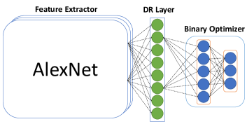
Fig. 1: Overview of the proposed end-to-end hashing framework.

Figure 1 illustrates the overall architecture of the proposed end-to-end deep hashing network. The network is composed of three major components: (i) a learning feature component which extracts visual image representations, (ii) a dimension reduction layer, and (iii) the hashing component which produces binary codes.

In CBIR systems, the feature extractor can be constructed from hand-crafted features [6] or learnable features such as convolutional neural networks [2]. In order to build an end-to-end system which can optimize all components, we choose the convolutional deep networks as the feature extractor. It is flexible that we can choose any convolutional deep networks such as VGG [16], AlexNet [17]. To make fair experiments, we utilize AlexNet as the feature extractor of the network for which is consistent with other hashing methods compared. In the proposed design, we remove the last layer (i.e. softmax layer) of AlexNet, and consider its last fully connected layer ($fc7$) as the image representation. Thus, the output of the feature extractor component is a 1024-dimensional real-valued vector.

The dimension reduction component (the DR layer) involves a fully connected layer initialized by PCA from the outputs of AlexNet’s $fc7$ layer from the training set. Specifically, let ${\mathbf{W}}_{PCA}$ and ${{\mathbf{b}}_{PCA}}$ be the weights and bias of the layer, respectively:

$${\mathbf{W}}_{PCA}=[{\mathbf{v}}_{1}^{T}\;{\mathbf{v}}_{2}^{T}\;\cdots\;{\mathbf{v}}_{p}^{T}]$$ (5)

$${\mathbf{b}}_{PCA}=-{\mathbf{W}}_{PCA}\mathbf{m}$$

where ${\mathbf{v}}_{1},{\mathbf{v}}_{2},\ldots,{\mathbf{v}}_{p}$ are eigenvectors extracted from the covariance matrix and $\mathbf{m}$ is the mean of the $fc7$ features of the training set ${\mathbf{X}}$. We use the identity function as the activation function of this layer.

The last component, namely the hashing optimizer, is constructed from several fully connected layers. The output of this component has the same length as the length of required binary output.

2.3 Training

Algorithm 1 End-to-End Supervised Hashing Deep Network Learning

1:

2:${\mathbf{X}}=\{{\mathbf{x}}_{i}\}_{i=1}^{n}$: training images; $L$: code length; $K$, $T$: maximum iteration; $m$: number of samples in a mini-batch.

3:

4:Network parameters ${\mathbf{W}}$

5:

6:Initialize the network ${\mathbf{W}}_{(0)}^{(0)}$ via the pretrained AlexNet

7:Initialize ${\mathbf{B}}^{(0)}\in\{-1,1\}^{L\times n}$ via ITQ [18]

8:for $k=1\to K$ do

9:    for $t=1\to T$ do

10:       A minibatch $X_{(t)}$ is sampled from ${\mathbf{X}}$

11:       Compute the corresponding similarity matrix ${\mathbf{S}}_{(t)}$

12:       From ${\mathbf{B}}^{(k-1)}$, sample $B_{(t)}$ corresponding to $X_{(t)}$

13:       Fix $B_{(t)}$, optimize ${\mathbf{W}}_{(t)}^{(k)}$ via SGD

14:    end for

15:    Update ${\mathbf{B}}^{(k)}=\text{sign}(f({\mathbf{W}}_{(T)}^{(k)},{\mathbf{X}}))$

16:end for

17:Return ${\mathbf{W}}_{(T)}^{(K)}$

The training procedure is demonstrated in Algorithm 1 in which ${\mathbf{B}}^{(k)}$ is the binary codes of the training set at $k$th iteration and ${\mathbf{W}}_{(t)}^{(k)}$ is SH-E2E’s parameters at the $t$th inner-loop of the $k$th outer-loop. First of all, we use a pretrained AlexNet as the initial weights of SH-E2E, namely ${\mathbf{W}}_{(0)}^{(0)}$. The DR layer is generated as discussed in Section 2.2 and the remaining layers are initialized randomly. In order to encourage the algorithm to converge faster, the binary variable ${\mathbf{B}}^{(0)}$ is initialized by ITQ [18].

We apply the alternating approach to minimize the loss function (4). In each iteration $t$, we only sample a minibatch $X_{(t)}$ including $m$ images from the training set as well as corresponding binary codes $B_{(t)}$ from ${\mathbf{B}}^{(k)}$. Additionally, we create the similarity matrix ${\mathbf{S}}_{(t)}$ (Equation 1) corresponding to $X_{(t)}$ as well as the $B_{(t)}$ matrix. Since $B_{(t)}\in\{-1,1\}^{L\times m}$ has been already computed, we can fix that variable and update the network parameter ${\mathbf{W}}_{(t)}^{(k)}$ by standard back-propagation via SGD. Through $T$ iterations, we are able to exhaustively use all training data. After learning SH-E2E from the whole training set, we update ${\mathbf{B}}^{(k)}=\text{sign}(f({\mathbf{W}}_{(T)}^{(k)},{\mathbf{X}}))$ and then start the optimization procedure again until it reaches a criterion, i.e., after $K$ iterations.

Comparing to the recent supervised hashing SH-BDNN [7], the proposed framework has two advantages. SH-E2E is an end-to-end hashing network which consists both feature extraction and binary code optimization in a unified framework. It differs from SH-BDNN which requires image features as inputs. Secondly, thanks to the SGD, SH-E2E can be trained with large scale datasets because the network builds the similarity matrix from an image batch of $m$ samples ($m\ll n$). It differs from SH-BDNN which uses the whole training set in each iteration.

3 Experiments

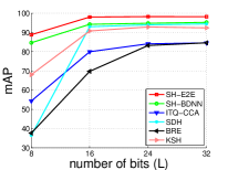
(a) MNIST

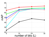
(b) Cifar10

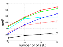
(c) SUN397

Fig. 2: mAP comparison between SH-E2E and other state-of-the-art methods on MNIST, Cifar10, SUN397.

3.1 Datasets

MNIST [19] comprises 70k grayscale images of 10 hand-written digits which are divided into 2 sets: 60k training images and 10k testing images.
Cifar10 [20] includes 60k RGB images categorized into 10 classes where images are divided into 50k training images and 10k testing images.
SUN397 [21] is a large-scale dataset which contains 108754 images categorized into 397 classes. Following the setting from [8], we select 42 categories which have more than 500 images. This results 35k images. For each class, we randomly sample 100 images as test samples and therefore we get 4200 images to form a testing set. The remaining images are considered as training samples.

3.2 Implementation details

We implement SH-E2E by MATLAB and the MatConvNet library [22]. All experiments are conducted in a workstation machine (Intel(R) Xeon(R) CPU E5-2650 2.20GHz) with one Titan X GPU. The last component includes 3 fully connected layer in which the sigmoid function is used as the activation function. The number of units in the binary optimizer are empirically selected as described in Table 1.

Table 1: The number of units in the binary optimizer.

$L$	Layer 1	Layer 2	Layer 3
8	90	20	8
16	90	30	16
24	100	40	24
32	120	50	32
48	140	80	48

Regarding the hyperparameters of the loss function, we finetune $\alpha$ in range $10^{-3}$ to $10^{-1}$, $\beta=10^{-2}$, $\gamma=10^{-2}$ and $\theta=10^{-3}$. For training the network, we select learning rate $lr=10^{-4}$ and weights decay to be $5\times 10^{-4}$. The size of a minibatch is $m=256$ for all experiments. Other settings in the algorithm are set as following: $K=5$, $T=\lceil\frac{4n}{m}\rceil$.

3.3 Comparison with other supervised hashing methods

We compare the proposed method with other supervised hashing methods, i.e., SH-BDNN [7], ITQ-CCA [18], KSH [23], BRE [24], SDH [25]. In order to make fair comparisons for other methods, follow [7], we use the pre-trained network AlexNet to extract features from fully connected layer $fc7$ then use PCA to map 4096-dimensional features to lower dimensional space, i.e., a 800 dimensional space. The reduced features are used as inputs for compared methods.

The comparative results between methods are shown in Fig. 2. On MNIST dataset, SH-E2E achieves fair improvements over compared methods. The performance of SH-E2E is saturated when the code lengths are higher than 16, i.e, its mAP are 98.03%, 98.26% and 98.21% at code length 16, 24, 32, respectively. The similar results can be observed on the Cifar10 dataset. As shown in Figure 2(b), SH-E2E outperforms other supervised hashing methods with a fair margin. SH-E2E outperforms the most competitive SH-BDNN from 4% to 7.5% at different code lengths. On the SUN397 dataset, SH-E2E and the second best SH-BDNN achieve comparable results, while these two methods significantly outperform other methods.

3.4 Comparison with other end-to-end hashing networks

We also compare the proposed deep network with other end-to-end supervised hashing architectures, i.e., Lai et al. [12], DHN [26], DQN [27], DSRH [28], and DRSCH [10]. For end-to-end networks comparisons, we follow two different settings for the MNIST and the Cifar10 datasets.

• Setting 1: according to [27, 26, 12], we randomly select 100 samples per class to form 1k testing images. The rest 59k images are database images. The training set contains 5k images which are sampled from the database (i.e., 500 images per class).

• Setting 2: following [10, 28], for test set, we sample 1k images for each class. This results 10k testing images. In the test phase, each test image is searched through the test set by the leave-one-out procedure. The rest 59k images are served as the training set.

The results of [12, 26, 10, 28, 27] are directly cited from the corresponding papers. Although those works proposed approaches which simultaneously learn image features and binary codes by combining CNN layers and a binary quantization layer, they used approximation of $sign$ function, i.e., [28] and  [12] use $logistic$ function, while [10] uses $tanh$ that may degrade the performance. Thanks to the new learning scheme for dealing with binary constraints and the effectiveness of proposed network architecture, the proposed SH-E2E outperforms other end-to-end methods with fair margins as observed in Table 2 and Table 3. Specifically, under Setting 1, the proposed SH-E2E and DHN [26] achieve comparable results while these two methods significantly outperform other methods. Under Setting 2, the proposed SH-E2E consistently outperforms the compared DRSCH [10] and DSRH [28] at all code lengths.

Table 2: mAP comparison between SH-E2E, DHN [26], DQN [27], and Lai et al.[12] on Cifar10 (Setting 1).

$L$	24	32	48
SH-E2E	60.02	61.35	63.59
DHN [26]	59.40	60.30	62.10
Lai et al.[12]	56.60	55.80	58.10
DQN [27]	55.80	56.40	58.00

Table 3: mAP comparison between SH-E2E, DRSCH[10] and DSRH [28] on Cifar10 (Setting 2).

$L$	24	32	48
SH-E2E	67.16	68.72	69.23
DRSCH [10]	62.19	62.87	63.05
DSRH [28]	61.08	61.74	61.77

4 Conclusions

We propose a new deep network architecture which efficiently learns compact binary codes of images. The proposed network comprises three components, i.e., feature extractor, dimension reduction and binary code optimizer. These components are trained in an end-to-end framework. In addition, we also propose the new learning scheme which can cope with binary constraints and also allows the network to be trained with large scale datasets. The experimental results on three benchmarks show the improvements of the proposed method over the state-of-the-art supervised hashing methods.

References

- [1] Thanh-Toan Do and Ngai-Man Cheung, “Embedding based on function approximation for large scale image search,” TPAMI, 2018.
- [2] Giorgos Tolias, Ronan Sicre, and Hervé Jégou, “Particular object retrieval with integral max-pooling of cnn activations,” 2016.
- [3] Kevin Lin, Jiwen Lu, Chu-Song Chen, and Jie Zhou, “Learning compact binary descriptors with unsupervised deep neural networks,” in CVPR, 2016, pp. 1183–1192.
- [4] Bohan Zhuang, Guosheng Lin, Chunhua Shen, and Ian Reid, “Fast training of triplet-based deep binary embedding networks,” in CVPR, 2016, pp. 5955–5964.
- [5] Jie Feng, Svebor Karaman, and Shih-Fu Chang, “Deep image set hashing,” in WACV. IEEE, 2017, pp. 1241–1250.
- [6] Thanh-Toan Do, Dang-Khoa Le Tan, Trung T. Pham, and Ngai-Man Cheung, “Simultaneous feature aggregating and hashing for large-scale image search,” in CVPR, July 2017.
- [7] Thanh-Toan Do, Anh-Dzung Doan, and Ngai-Man Cheung, “Learning to hash with binary deep neural network,” in ECCV. Springer, 2016, pp. 219–234.
- [8] Thanh-Toan Do, Anh-Dzung Doan, Duc-Thanh Nguyen, and Ngai-Man Cheung, “Binary hashing with semidefinite relaxation and augmented lagrangian,” in ECCV. Springer, 2016, pp. 802–817.
- [9] Jun Wang, Wei Liu, Sanjiv Kumar, and Shih-Fu Chang, “Learning to hash for indexing big data—a survey,” Proceedings of the IEEE, vol. 104, no. 1, pp. 34–57, 2016.
- [10] Ruimao Zhang, Liang Lin, Rui Zhang, Wangmeng Zuo, and Lei Zhang, “Bit-scalable deep hashing with regularized similarity learning for image retrieval and person re-identification,” TIP, pp. 4766–4779, 2015.
- [11] Venice Erin Liong, Jiwen Lu, Gang Wang, Pierre Moulin, and Jie Zhou, “Deep hashing for compact binary codes learning,” in CVPR, 2015.
- [12] Hanjiang Lai, Yan Pan, Ye Liu, and Shuicheng Yan, “Simultaneous feature learning and hash coding with deep neural networks,” in CVPR, 2015, pp. 3270–3278.
- [13] Geoffrey E Hinton, Simon Osindero, and Yee-Whye Teh, “A fast learning algorithm for deep belief nets,” Neural computation, vol. 18, no. 7, pp. 1527–1554, 2006.
- [14] Haomiao Liu, Ruiping Wang, Shiguang Shan, and Xilin Chen, “Deep supervised hashing for fast image retrieval,” in CVPR, 2016, pp. 2064–2072.
- [15] Jorge Nocedal and Stephen J. Wright, Numerical Optimization, Chapter 17, World Scientific, 2nd edition, 2006.
- [16] K. Simonyan and A. Zisserman, “Very deep convolutional networks for large-scale image recognition,” CoRR, vol. abs/1409.1556, 2014.
- [17] Alex Krizhevsky, Ilya Sutskever, and Geoffrey E Hinton, “Imagenet classification with deep convolutional neural networks,” in NIPS, 2012, pp. 1097–1105.
- [18] Yunchao Gong and Svetlana Lazebnik, “Iterative quantization: A procrustean approach to learning binary codes,” in CVPR, 2011.
- [19] Yann Lecun and Corinna Cortes, “The MNIST database of handwritten digits,” http://yann.lecun.com/exdb/mnist/.
- [20] Alex Krizhevsky, “Learning multiple layers of features from tiny images,” Tech. Rep., University of Toronto, 2009.
- [21] Jianxiong Xiao, James Hays, Krista A Ehinger, Aude Oliva, and Antonio Torralba, “Sun database: Large-scale scene recognition from abbey to zoo,” in CVPR. IEEE, 2010, pp. 3485–3492.
- [22] A. Vedaldi and K. Lenc, “Matconvnet – convolutional neural networks for matlab,” in ACM Multimedia, 2015.
- [23] Wei Liu, Jun Wang, Rongrong Ji, Yu-Gang Jiang, and Shih-Fu Chang, “Supervised hashing with kernels,” in CVPR. IEEE, 2012, pp. 2074–2081.
- [24] Brian Kulis and Trevor Darrell, “Learning to hash with binary reconstructive embeddings,” in NIPS, 2009, pp. 1042–1050.
- [25] Fumin Shen, Chunhua Shen, Wei Liu, and Heng Tao Shen, “Supervised discrete hashing,” in CVPR, 2015.
- [26] Han Zhu, Mingsheng Long, Jianmin Wang, and Yue Cao, “Deep hashing network for efficient similarity retrieval.,” in AAAI, 2016, pp. 2415–2421.
- [27] Yue Cao, Mingsheng Long, Jianmin Wang, Han Zhu, and Qingfu Wen, “Deep quantization network for efficient image retrieval.,” in AAAI, 2016, pp. 3457–3463.
- [28] Fang Zhao, Yongzhen Huang, Liang Wang, and Tieniu Tan, “Deep semantic ranking based hashing for multi-label image retrieval,” in CVPR, 2015.