Singlet-Triplet Fermionic Dark Matter and LHC Phenomenology

Abstract

It is well known that for the pure standard model triplet fermionic WIMP-type dark matter (DM), the relic density is satisfied around 2 TeV. For such a heavy mass particle, the production cross-section at 13 TeV run of LHC will be very small. Extending the model further with a singlet fermion and a triplet scalar, DM relic density can be satisfied for even much lower masses. The lower mass DM can be copiously produced at LHC and hence the model can be tested at collider. For the present model we have studied the multi jet ($\geq 2\,j$) + missing energy ($\cancel{E}_{T}$) signal and show that this can be detected in the near future of the LHC 13 TeV run. We also predict that the present model is testable by the earth based DM direct detection experiments like Xenon-1T and in future by Darwin.

I Introduction

The Standard Model (SM) of elementary particles is a very well established and successful theory. With the discovery of the Higgs boson at the LHC, the last missing piece of the SM has been found. So far, all observations at the collider experiments are reasonably consistent with the SM cementing its position even further. However, despite this success story it is well accepted that the SM is not the full theory of nature. Rather, SM is widely looked as a low energy effective limit of a more complete underlying theory. The reasons to believe that SM needs to be extended are both theoretical as well as observational. Amongst the most compelling observational evidences of physics Beyond the SM (BSM) is the issue of the Dark Matter (DM). The DM, if it is a particle, should be massive, chargeless and weakly interacting such that its relic abundance should be consistent with the observational data on DM. The SM fails to provide any such candidate. The only weakly interacting chargeless particle in the SM is the neutrino and it is postulated to be massless. Of course experimental data have now given conclusive evidence that neutrinos are massive - which is another compelling reason to extend the SM to accommodate neutrino mass. However neutrinos, even if massive in a BSM theory, can only be hot dark matter candidate and it is well known that hot dark matter is inconsistent with structure formation of the universe. Therefore, we need a BSM theory that can provide either cold or warm dark matter candidate.

Presence of DM is a very well established fact which is supported by many evidences. The first evidence of DM came from the observation of the flatness of the rotation curve of the Coma cluster by a Swedish scientist, Zwicky, in 1930 Sofue:2000jx . Other strong evidences that support the DM theory include gravitational lensing Bartelmann:1999yn , recent observation of bullet cluster by NASA’s Chandra satellite Clowe:2003tk ; Harvey:2015hha , and from the measurement of Cosmic Microwave Background (CMB) radiation Hinshaw:2012aka ; Ade:2015xua . Planck Hinshaw:2012aka and WMAP Ade:2015xua have precisely measured the amount of DM present in the universe and have given a $2\sigma$ bound on the DM relic density as,

$$\Omega h^{2}=0.1199\pm 0.0027$$ (1)

Many different classes of DM candidates like the Weakly Interacting Massive Particle (WIMP), Strongly Interacting Massive Particle (SIMP) and Feebly Interacting Massive Particle (FIMP), have been proposed in the literature. Each type can solve the DM puzzle in its unique way. In this work we will consider a model with a WIMP-type fermionic DM candidate by extending the SM particle spectrum and study in detail the DM phenomenology. We will also study the collider signal of the DM at the 13 TeV run of the LHC and its effect will basically manifest as the missing energy associated with hard jets. In Hisano:2002fk ; Hisano:2003ec ; Hisano:2004ds ; Cirelli:2005uq ; Hisano:2006nn ; Ma:2008cu ; Cohen:2013ama , a model has been proposed where the fermionic DM belongs to the triplet representation of the SM. An extra discrete $\mathbb{Z}_{2}$ symmetry stabilizes the DM making the neutral part of the triplet fermion as the viable candidate for the DM. If the SM is extended by only the triplet fermion Cirelli:2005uq ; Ma:2008cu , then the main co-annihilation processes take part in the DM relic density calculation are mediated by the charged gauge boson $W^{\pm}$, and for this case the correct value of DM relic density is obtained for DM mass around 2.3 TeV Cirelli:2005uq ; Ma:2008cu . This high mass makes it difficult to produce the purely triplet fermionic DM at the 13 TeV collider, and hence to test this model at the LHC. Of course with a higher energy collider one might be able to to produce these heavy fermions. Another major drawback of such high mass DM is that when the DM annihilate to gamma rays via $W^{\pm}$-mediated one loop diagrams, then for such high DM mass, the annihilation is increased by the Sommerfeld enhancement (SE) factor Hisano:2003ec ; Hisano:2004ds ; Cirelli:2005uq . This is ruled out from the indirect search of the HESS data Abramowski:2013ax . In this paper, we propose an extension of the SM that accommodates both high as well as low mass fermionic DM such that it can be produced and tested at the 13 TeV run of the LHC. The low mass DM regime do not have any significant SE enhancement (because the DM mass becomes comparable to the mediator mass inside the loops) and hence are safe from the gamma ray indirect detection bounds put by the Fermi-LAT collaboration Ackermann:2015lka . Our proposed extension of the particle content includes one SM singlet fermion and SM triplet fermion Chardonnet:1993wd ; Biggio:2011ja ; Hirsch:2013ola ; Chaudhuri:2015pna ; Bhattacharya:2017sml . The scalar sector is also extended to include a SM triplet scalar. The $\mathbb{Z}_{2}$ charge of these BSM particles is arranged in such a way that there is a mixing between the neutral component of the triplet fermion and the singlet fermion, that generates two mass eigenstates for the neutral fermions. The lower mass eigenstate becomes the viable DM candidate. The neutral and charged components of the SM doublet and triplet scalars also mix, that gives rise to two physical neutral Higgs scalars and one charged Higgs scalar. The presence of these extra scalars opens up additional annihilation and co-annihilation processes between the two DM candidates which effectively reduces the mass of the DM for which the current DM relic density bound can be easily satisfied. For low mass DM we give the prediction for the annihilation of the DM to two gamma rays by one loop process. In addition, these lower mass DM fermions ($\sim$ 100 GeV) can be observed with large production cross-section at the 13 TeV LHC. We perform a detailed collider phenomenology of the DM model. In this work we will consider multi jets + missing energy signal in the final state for searching the DM. We study in detail the dominant backgrounds for such type of signal. The SM backgrounds are reduced by applying suitable cuts that increases the statistical significance of detection for the fermionic DM with the low luminosity run of the LHC. A final comment is in order. It is possible to embed our model in a SO(10) GUT where the SU(2) triplet would belong to the 45 representation of SO(10) and would help in the gauge coupling unification, as was shown in Frigerio:2009wf ; Mambrini:2016dca .

Rest of the manuscript is organised as follows. In section II we briefly discuss the triplet fermionic DM model proposed in Cirelli:2005uq ; Ma:2008cu and its corresponding DM constraints. In section III we details of our proposed model. In section IV we list down all the constraints imposed on the DM model parameter space from the existing data. In section V we present our main results on the DM phenomenology of our model. In section VII, we show the predicted gamma ray flux from our model and compare it against the bounds from the Fermi-LAT data. In section VIII we study in detail the collider phenomenology of our model for the 13 TeV LHC. Finally, we summarise our results in section IX.

II Triplet Fermionic Dark Matter

Gauge Group $SU(3)_{c}$ $SU(2)_{L}$ $U(1)_{Y}$ $\mathbb{Z}_{2}$

Baryon Fields $Q_{L}^{i}=(u_{L}^{i},d_{L}^{i})^{T}$ $u_{R}^{i}$ $d_{R}^{i}$ $3$ $3$ $3$ $2$ $1$ $1$ $1/6$ $2/3$ $-1/3$ $+$ $+$ $+$

Lepton Fields $L_{L}^{i}=(\nu_{L}^{i},e_{L}^{i})^{T}$ $e_{R}^{i}$   $\rho$ $1$ $1$ $1$ $2$ $1$ $3$ $-1/2$ $-1$ $0$ $+$ $+$ $-$

Scalar Fields $\phi_{h}$ $1$ $2$ $1/2$ $+$

Table 1: Particle content and their corresponding charges under various symmetry groups.

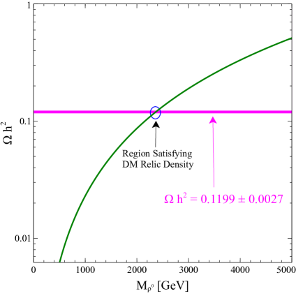
Figure 1: Variation of relic density $\Omega h^{2}$ with the mass of the triplet DM $M_{\rho^{0}_{1}}$.

In this case the SM particle content is extended with just a left handed fermionic triplet field $\rho$ Cirelli:2005uq ; Ma:2008cu . There is an additional $\mathbb{Z}_{2}$ symmetry imposed on the model such that the triplet is odd under it, while all SM particles are even under this symmetry. The particle content of the model and their charges under the symmetries of the model is given in Table 1. The $\mathbb{Z}_{2}$ symmetry forbids all the Yukawa couplings of $\rho$ with the SM fermions and the complete Lagrangian includes just the additional kinetic energy term for the triplet ($\mathcal{L}_{\rho}$) along with the SM Lagrangian ($\mathcal{L_{SM}}$),

$$\mathcal{L}=\mathcal{L_{SM}}+\mathcal{L}_{\rho}\,.$$ (2)

The Lagrangian for triplet field $\rho$ takes the following form,

$$\mathcal{L}_{\rho}=Tr[\bar{\rho}\,i\gamma^{\mu}D_{\mu}\,\rho]\,,$$ (3)

where the covariant derivative $D_{\mu}$ takes the following form,

$$D_{\mu}=\partial_{\mu}-ig\,T^{adj}_{i}\,W_{i}\,,$$ (4)

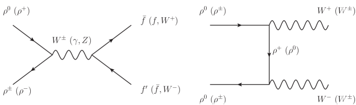
Figure 2: Pure triplet fermions DM annihilation and co-annihilation diagrams.

where $g$ and $W_{i}$ are the $SU(2)_{L}$ gauge coupling and gauge field, respectively, and $T^{adj}_{i}$’s are the $SU(2)_{L}$ generators in the adjoint representation. The $\mathbb{Z}_{2}$ symmetry makes $\rho^{0}$, the chargeless component of $\rho$ stable and it becomes the DM. The annihilation and co-annihilation of the DM $\rho_{0}$, and $\rho^{\pm}$ proceed through SM gauge bosons, as shown in Fig. 2. In Fig. 1 we show the $\rho^{0}$ relic abundance as a function of its mass $M_{\rho^{0}}$. From the figure one can notice that with the increase of the DM mass, its relic density also increases. This is because in the present case the velocity times the DM annihilation and co-annihilation cross sections vary inversely with the square of the DM mass. Hence, as the DM mass is increased, the DM annihilation cross-section decreases and as a result the DM relic density increases as it is inversely proportional to the velocity times cross section. From the figure we note that the present day observed value of the DM relic density is satisfied around $M_{\rho^{0}}\sim 2370$ GeV. This has been also pointed out before in Ma:2008cu .

Note that, while the model can be tested in direct and indirect detection experiments, due to its heavy mass it is difficult to produce this DM candidate at the 13 TeV or 14 TeV LHC search. One will need a very high energy collider to test this DM model. Minimal extension of the model by adding a gauge singlet fermion and a triplet scalar opens up the possibility to test the model at collider. Below, we discuss in detail the required extensions and the model predictions.

III Singlet Triplet Mixing

Gauge Group $SU(3)_{c}$ $SU(2)_{L}$ $U(1)_{Y}$ $\mathbb{Z}_{2}$

Baryon Fields $Q_{L}^{i}=(u_{L}^{i},d_{L}^{i})^{T}$ $u_{R}^{i}$ $d_{R}^{i}$ $3$ $3$ $3$ $2$ $1$ $1$ $1/6$ $2/3$ $-1/3$ $+$ $+$ $+$

Lepton Fields $L_{L}^{i}=(\nu_{L}^{i},e_{L}^{i})^{T}$  $e_{R}^{i}$  $N^{\prime}$  $\rho$ $1$ $1$ $1$ $1$ $2$ $1$ $1$ $3$ $-1/2$ $-1$ $0$ $0$ $+$ $+$ $-$ $-$

Scalar Fields $\phi_{h}$ $\Delta$   $1$ $1$   $2$ $3$   $1/2$ $0$   $+$ $+$

Table 2: Particle content and their corresponding charges under various symmetry groups.

In this section, we present a minimal extension of the model, such that the mass of the DM can be suitably reduced and it can be produced at the LHC. To that end, we add an extra gauge singlet fermion which is also odd under the $\mathbb{Z}_{2}$ and an additional real triplet Higgs ($Y=0$). The particle content of our model and their respective charges are displayed in the Table 2. The corresponding Lagrangian is given by,

$$\mathcal{L} = \mathcal{L}_{SM}+Tr\left[\bar{\rho}\,i\,\gamma^{\mu}D_{\mu}\rho\right]+\bar{N^{\prime}}\,i\,\gamma^{\mu}D_{\mu}N^{\prime}+Tr[(D_{\mu}\Delta)^{\dagger}(D^{\mu}\Delta)]-V(\phi_{h},\Delta)$$ (5)

$$-Y_{\rho\Delta}\,(Tr[\bar{\rho}\,\Delta]\,N^{\prime}+h.c.)-M_{\rho}\,Tr[\bar{\rho^{c}}\rho]-M_{N^{\prime}}\,\bar{N^{\prime c}}N^{\prime}$$

where the triplet fermion takes the following form,

$$\rho=\begin{pmatrix}\frac{\rho_{0}}{2}&\frac{\rho^{+}}{\sqrt{2}}\\ \frac{\rho^{-}}{\sqrt{2}}&-\frac{\rho_{0}}{2}\end{pmatrix}\,\,.$$ (6)

The complete form of the potential $V(\phi_{h},\Omega)$ takes the following form,

$$V(\phi_{h},\Delta) = -\mu_{h}^{2}\phi_{h}^{\dagger}\phi_{h}+\frac{\lambda_{h}}{4}(\phi_{h}^{\dagger}\phi_{h})^{2}+\mu_{\Delta}^{2}Tr[\Delta^{\dagger}\Delta]+\lambda_{\Delta}(\Delta^{\dagger}\Delta)^{2}+\lambda_{1}\,(\phi_{h}^{\dagger}\phi_{h})\,{\rm Tr}\,[\Delta^{\dagger}\Delta]$$ (7)

$$+\lambda_{2}\,\left(Tr[\Delta^{\dagger}\Delta]\right)^{2}+\lambda_{3}\,Tr[(\Delta^{\dagger}\Delta)^{2}]+\lambda_{4}\,\phi_{h}^{\dagger}\Delta\Delta^{\dagger}\phi_{h}+(\mu\phi_{h}^{\dagger}\Delta\phi_{h}+h.c.)\,.$$

In general, one can also insert a term like $\phi_{h}^{\dagger}\Delta^{\dagger}\Delta\phi_{h}$, but this term can be easily decomposed to two components that give contribution to the terms with $\lambda_{1}$ and $\lambda_{4}$ couplings. Hence, we do not write this term separately in the potential. We assume here that $\mu_{\Delta}^{2}$ is positive hence the neutral component of the Higgs triplet will get small induced vev, because it has coupling with the SM like Higgs, after electro weak symmetry breaking (EWSB) which takes the following form,

$$\langle\Delta_{0}\rangle=v_{\Delta}=\frac{\mu v^{2}}{2\left(\mu_{\Delta}^{2}+(\lambda_{4}+2\lambda_{1})\frac{v^{2}}{4}+(\lambda_{3}+2\lambda_{2})\frac{v_{\Delta}^{2}}{2}\right)}$$ (8)

The Higgs doublet and real triplet take the following form after taking the small fluctuation around the vevs $v$ and $v_{\Delta}$, respectively,

$$\phi_{h}=\begin{pmatrix}\phi^{+}\\ \dfrac{v+H+i\,\xi}{\sqrt{2}}\end{pmatrix}\,\,\,\,\,\,\,\,\,\,\,\,\Delta=\begin{pmatrix}\frac{\Delta_{0}+v_{\Delta}}{2}&\frac{\Delta^{+}}{\sqrt{2}}\\ \frac{\Delta^{-}}{\sqrt{2}}&-\frac{\Delta_{0}+v_{\Delta}}{2}\end{pmatrix}\,\,.$$ (9)

Since $\phi_{h}$ takes vev spontaneously which breaks the EWSB and $\Delta$ gets induced vev, we need to satisfy the following criterion for the quadratic and quartic couplings,

$$\mu_{h}^{2}>0,\,\,\,\,\mu_{\Delta}^{2}>0,\,\,\,\,\lambda_{h}>0\,\,\,\,{\rm and}\,\,\,\,\lambda_{\Delta}>0\,.$$ (10)

After symmetry breaking the $2\times 2$ mass matrix for the CP even Higgs scalars $H$ and $\Delta_{0}$ take the following form,

$$M_{s}=\frac{1}{2}\begin{pmatrix}\lambda\,v^{2}&v\,v_{\Delta}(2\lambda_{1}+\lambda_{4})-2\,\mu\,v\\ v\,v_{\Delta}(2\lambda_{1}+\lambda_{4})-2\,\mu\,v&2\,v_{\Delta}^{2}(\lambda_{3}+2\lambda_{2})+\frac{\mu\,v^{2}}{v_{\Delta}}\end{pmatrix}$$ (11)

After diagonalisation of the above matrix we will get the physical Higgses $h_{1}$ and $h_{2}$ with masses $M_{h_{1}}$ and $M_{h_{2}}$, respectively. If the mixing angle between $h_{1}$ and $h_{2}$ is $\alpha$, then the mass and flavor eigenstates can be written in the following way,

$$h_{1} = \cos\alpha\,H+\sin\alpha\,\Delta_{0}$$

$$h_{2} = -\sin\alpha\,H+\cos\alpha\,\Delta_{0}$$ (12)

The CP odd field $\xi$ becomes Goldstone boson which is “eaten” by the SM gauge boson $Z$. In addition to the mixing between $H$ and $\Delta_{0}$, the charged scalars will also be mixed and one of them will be the Goldstone boson “eaten” by $W^{\pm}$. We can write them in the physical basis in the following way,

$$G^{\pm} = \cos\delta\,\phi^{\pm}+\sin\delta\,\Delta^{\pm}$$

$$H^{\pm} = -\sin\delta\,\phi^{\pm}+\cos\delta\,\Delta^{\pm}$$ (13)

where the mixing angle depends on the strength of the vevs of doublet and triplet, i.e.,

$$\tan\delta=\frac{2\,v_{\Delta}}{v}\,.$$ (14)

The quadratic and quartic couplings have the following form in terms of the CP even Higgs masses $M_{h_{1}}$ and $M_{h_{2}}$, the mixing angle between them $\alpha$, the charge scalar mass and the mixing angle between the charged scalars $\delta$:

$$\mu = \frac{M_{H^{\pm}}^{2}\sin\delta\cos\delta}{v}\,,$$

$$\lambda_{3}+2\,\lambda_{2} = \dfrac{M_{h_{1}}^{2}+M_{h_{2}}^{2}+(M_{h_{2}}^{2}-M_{h_{1}}^{2})\cos 2\alpha-2\,M_{H^{\pm}}^{2}\cos^{2}\delta}{2\,v_{\Delta}^{2}}\,,$$

$$\lambda_{h} = \dfrac{M_{h_{1}}^{2}+M_{h_{2}}^{2}+(M_{h_{1}}^{2}-M_{h_{2}}^{2})\cos 2\alpha}{v^{2}},$$

$$\lambda_{4}+2\,\lambda_{1} = \dfrac{(M_{h_{1}}^{2}-M_{h_{2}}^{2})\sin 2\alpha+M^{2}_{H^{\pm}}\sin 2\,\delta}{v\,v_{\Delta}}\,,$$

$$\mu_{h}^{2} = \lambda_{h}\,\frac{v^{2}}{4}+(\lambda_{4}+2\lambda_{1})\,\frac{v_{\Delta}^{2}}{4}-\mu\,v_{\Delta}\,.$$ (15)

The vev of the Higgs triplet is constrained by the data on the ratio $\frac{M_{W}^{2}}{\cos^{2}\theta_{w}M_{Z}^{2}}$, which limits $v_{\Delta}<12$ GeV Erler:2004nh ; Erler:2008ek . The value of $M_{h_{2}}$ needs to satisfy the perturbativity limit on the quartic couplings which is $\lambda<4\pi$. The quartic couplings are also bounded from the below Chen:2008jg and as long as all the quartic couplings are positive, we do not need to worry about the lower bounds. From Eq. (15) we see that by choosing a suitable value for the free parameter $\mu$ which has mass dimension, we can keep all the quartic couplings in the perturbative regime.

In Eq. (5), $Y_{\rho\Delta}$ is the Yukawa term relating the fermionic triplet with the fermionic singlet. When the neutral component of $\Delta$ takes vev, the mass matrix for the fermions takes the following form,

$$M_{F}=\begin{pmatrix}M_{\rho}&\frac{Y_{\rho\Delta}v_{\Delta}}{2}\\ \frac{Y_{\rho\Delta}v_{\Delta}}{2}&M_{N^{\prime}}\end{pmatrix}\,.$$ (16)

The lightest component of the eigenvalues of this matrix will be the stable DM. Relation between the the mass eigenstates and weak eigenstates are as follows:

$$\rho_{2}^{0} = \cos\beta\,\rho_{0}+\sin\beta\,N^{\prime c}$$

$$\rho_{1}^{0} = -\sin\beta\,\rho_{0}+\cos\beta\,N^{\prime c}$$ (17)

Therefore, the tree level mass eigenstates are,

$$M_{\rho_{1}^{0}} = \frac{1}{2}\left(M_{\rho}+M_{N^{\prime}}-\sqrt{(M_{\rho}-M_{N^{\prime}})^{2}+4\left(\frac{Y_{\rho\Delta}v_{\Delta}}{2}\right)^{2}}\right)\,,$$

$$M_{\rho_{2}^{0}} = \frac{1}{2}\left(M_{\rho}+M_{N^{\prime}}+\sqrt{(M_{\rho}-M_{N^{\prime}})^{2}+4\left(\frac{Y_{\rho\Delta}v_{\Delta}}{2}\right)^{2}}\right)\,,$$

$$\tan 2\beta = \frac{Y_{\rho\Delta}v_{\Delta}}{M_{\rho}-M_{N^{\prime}}}\,.$$ (18)

In terms of $M_{\rho_{1}^{0}}$ and $M_{\rho_{2}^{0}}$ we can express the Yukawa coupling $Y_{\rho\Delta}$ in the following way:

$$Y_{\rho\Delta} = \frac{(M_{\rho_{2}^{0}}-M_{\rho_{1}^{0}})\sin 2\beta}{2\,v_{\Delta}}\,,$$ (19)

$$= \frac{\Delta M_{21}\sin 2\beta}{2v_{\Delta}}$$

where $\Delta M_{21}=(M_{\rho_{2}^{0}}-M_{\rho_{1}^{0}})$ represents the mass difference between $M_{\rho_{2}^{0}}$ and $M_{\rho_{1}^{0}}$. Therefore, one can increase the Yukawa coupling $Y_{\rho\Delta}$ by increasing the mass difference $\Delta M_{21}$ or the singlet triplet fermionic mixing angle, or decreasing the triplet vev $v_{\Delta}$. We have kept the mass of charged component ($\rho^{\pm}$) of triplet fermion equal to the mass of $\rho_{2}^{0}$ with the mass gap of pion i.e. $M_{\rho^{\pm}}=M_{\rho_{2}^{0}}+0.16$ GeV.

A further discussion is in order. For the present model we can generate the neutrino mass by Type I seesaw mechanism just by introducing SM singlet right handed neutrinos. In other variants of the triplet fermionic DM model, neutrino masses were generated by using the Type III seesaw mechanism and radiatively by the authors of Abada:2008ea and Ma:2008cu ; Chardonnet:1993wd ; Biggio:2011ja ; Hirsch:2013ola , respectively.

IV Constraints used in Dark Matter Study

Below, we discuss different constraints that we take into account. This includes the constraints from relic density, the direct detection constraints, as well as the invisible Higgs decay.

IV.1 SI direct detection cross section

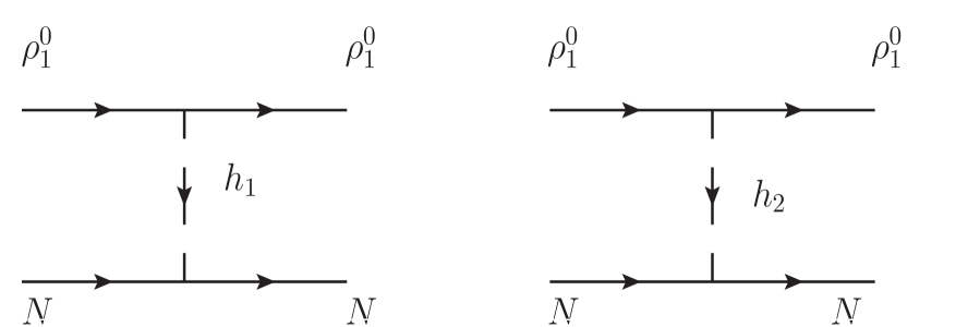
Figure 3: SI direct detection scattering processes between DM and nucleaon of the nucleus.

The Feynman diagrams in Fig. 3 show the spin independent (SI) direct detection (DD) scattering processes between the DM and the nucleon ($\rho^{0}_{1}\,N\rightarrow\rho^{0}_{1}\,N$), which are mediated by the two Higgses $h_{1}$ and $h_{2}$, respectively, through the t-channel process. Since DM interacts very weakly with the nucleon, one can safely calculate the cross-section for this process in the $t\rightarrow 0$ limit, where $t$ is the Mandelstam variable corresponding to the square of the four-momentum transfer. The expression for the above process takes the following form,

$$\sigma_{SI} = \frac{\mu_{red}^{2}}{\pi}\,\left[\frac{M_{N}f_{N}}{v}\left(\frac{g_{\rho^{0}_{1}\rho^{0}_{1}h_{2}}\sin\alpha}{M_{h_{2}}^{2}}-\frac{g_{\rho^{0}_{1}\rho^{0}_{1}h_{1}}\cos\alpha}{M_{h_{1}}^{2}}\right)\right]^{2}$$ (20)

where the quantity $f_{N}$ is the nucleon form factor and it is equal to $0.3$ Belanger:2008sj while $\mu_{red}$ is the reduced mass between the DM mass ($M_{\rho^{0}_{1}}$) and the nucleon mass ($M_{N}$) and is given by

$$\mu_{red} = \frac{M_{N}M_{\rho^{0}_{1}}}{M_{N}+M_{\rho^{0}_{1}}}\,,$$ (21)

The couplings in Eq. (20) $g_{\rho^{0}_{1}\rho^{0}_{1}h_{1}}$ and $g_{\rho^{0}_{1}\rho^{0}_{1}h_{2}}$ are given by,

$$g_{\rho^{0}_{1}\rho^{0}_{1}h_{1}} = \frac{Y_{\rho\Delta}}{2}\sin 2\beta\,\sin\alpha\,,$$

$$g_{\rho^{0}_{1}\rho^{0}_{1}h_{2}} = \frac{Y_{\rho\Delta}}{2}\sin 2\beta\,\cos\alpha\,,$$ (22)

where $Y_{\rho\Delta}$, $\alpha$ and $\beta$ have been defined in the previous section. We had seen in Eq. (19) that the Yukawa coupling $Y_{\rho\Delta}$ is linearly proportional to $\sin 2\beta$ for a given choice of mass splitting $\Delta M_{21}=(M_{\rho^{0}_{2}}-M_{\rho^{0}_{1}})$ and vev $v_{\Delta}$. Therefore, inserting Eqs. (19) and (22) into Eq. (20) we get

$$\sigma_{SI} = \frac{\mu_{red}^{2}}{\pi}\,\left[\frac{M_{N}f_{N}}{v}\frac{\Delta M_{21}\,\sin^{2}2\beta\,\sin 2\alpha}{4v_{\Delta}}\left(\frac{1}{M_{h_{2}}^{2}}-\frac{1}{M_{h_{1}}^{2}}\right)\right]^{2}$$ (23)

Since $\sigma_{SI}$ depends on the model parameters, and since the current limit from DD experiments need to be satisfied, they put a constraint on the our model parameter space. Also, the model could be tested and/or the parameter space can be constrained by the future DD experiments like LUX Akerib:2015rjg ; Akerib:2016vxi , Xenon-1T Aprile:2015uzo ; Aprile:2017iyp , Panda Cui:2017nnn and Darwin Aalbers:2016jon .

IV.2 Invisible decay width of Higgs

If the DM candidate has mass less than half the SM-like Higgs mass then the SM-like Higgs could decay to pair of DM particles. This process would contribute to the decay width of the SM-like Higgs into invisible states. The Higgs decay width has been measured very precisely by the LHC which constrains the Higgs decay in such a way that its branching ratio to invisible states must be less than 34$\%$ at 95$\%$ C.L. Khachatryan:2016vau . In the present model the Higgs decay width to invisible states $\rho_{1}^{0}$ (since in the present work $M_{\rho_{2}^{0}}>\frac{M_{h_{1}}}{2}$, hence Higgs can not decay to $\rho_{2}^{0}$) is given by,

$$\Gamma_{h_{1}\rightarrow\rho_{1}^{0}\rho_{1}^{0}}=\frac{M_{h_{1}}g_{\rho_{1}^{0}\rho_{1}^{0}h_{1}}^{2}}{16\pi}\left(1-\frac{4M_{\rho_{1}^{0}}^{2}}{M_{h_{1}}^{2}}\right)^{3/2}\,,$$ (24)

where $g_{\rho_{1}^{0}\rho_{1}^{0}h_{1}}$ is given in Eq. (22). In order to satisfy the LHC limit, the model parameters have to satisfy the following constraint

$$\frac{\Gamma_{h_{1}\rightarrow\rho_{1}^{0}\rho_{1}^{0}}}{\Gamma_{h_{1}}^{Total}}\leq 34\%{\rm\,\,at\,\,\,95\%\,\,\,C.L.}$$ (25)

For the parameter range where the kinematical condition $M_{\rho_{1}^{0}}<\frac{M_{h_{1}}}{2}$ is satisfied we impose the condition given by Eq. (25) and only model parameter values that satisfy this constraints are used in our analysis.

IV.3 Planck Limit

Relic density for the DM has been measured very precisely by the satellite borne experiments WMAP Hinshaw:2012aka and Planck Ade:2015xua . In this work we have used the following bound on the DM relic density,

$$0.1172\leq\Omega h^{2}\leq 0.1226{\rm\,\,\,at\,\,68\%\,\,C.L.}\,,$$ (26)

which is used to constrain the model parameters such that it is compatible with the Planck limit on DM abundance.

V Dark Matter Relic Abundance

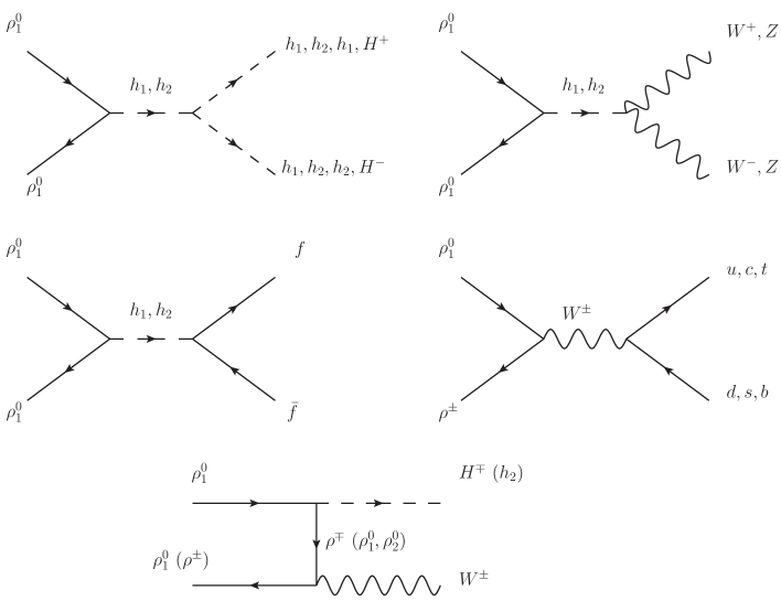
Figure 4: Feynman diagrams which dominantly participate in determining the relic density of DM.

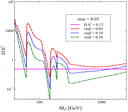
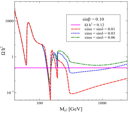
Figure 5: Left Panel: variation of DM relic density for three different values of the singlet triplet fermionic mixing angle $\sin\beta$. Right Panel: variation of DM relic density for three different values of the neutral Higgses mixing angle $\sin\alpha$. When the BSM Higgs value kept fixed at $M_{h_{2}}=300$ GeV and we took $\sin\delta$ equal neutral Higgs mixing angle for simplicity and kept the mass difference $\Delta M_{12}$ fixed at 50 GeV.

In analysing the DM phenomenology we implement the model in Feynrules Alloul:2013bka . We generate Calchep files using Feynrules and feed the output files into micrOmegas Belanger:2013oya . The relevant Feynman diagrams that determine the DM relic abundance are shown in Fig. 4. In presence of triplet as well as singlet states, additional channels mediated by the neutral and charged Higgs state opens up.

Different model parameters, such as, the mass of DM, neutral Higgs, mixing between singlet and triplet fermions, as well as different Higgs states can impact the DM relic density. We analyse the dependence of the DM relic density on the model parameters and also study the correlation between them that follows from the DM relic density constraint. Fig. 5 shows the variation w.r.t the mass of DM taking into account the variation of the different mixing angles. In other figures, such as, Fig. 6, we explore the dependency on the mass-difference and the BSM Higgs masses. Few comments are in order:

• In the left panel (LP) of Fig. 5, we show the variation of the DM relic density with DM mass for three different values of the singlet-triplet mixing angle $\sin\beta$. The thin magenta band shows the $2\sigma$ experimentally allowed range of the DM relic density reported by the Planck collaboration. From the figure, this is evident, that there are four dip regions with respect to the DM mass. The first resonance occurs at $M_{\rho_{1}^{0}}\simeq M_{h_{1}}/2\sim 62.5$ GeV. The SM-like Higgs mediated diagrams shown in Fig. 4 give the predominant contribution in this mass range. The second resonance occurs at $M_{\rho_{1}^{0}}\sim 150$ GeV, when the DM mass is approximately half the BSM Higgs mass ($M_{\rho_{1}^{0}}\simeq M_{h_{2}}/2$) assumed in this figure. The third dip is due to the t-channel diagram $\rho_{1}^{0}\,\rho_{1}^{0}\rightarrow W^{\pm}H^{\mp}$ mediated by the $\rho^{\pm}$. This dip occurs when the DM mass satisfies the relation $M_{\rho_{1}^{0}}=\frac{M_{W^{\pm}}+M_{H^{\mp}}}{2}$ and happens due to the destructive interference term of the $W^{\pm}H^{\mp}$ final state. The fourth dip happens because of the threshold effect of the $W^{\pm}H^{\mp}$ final state and clear from the fact that with the variation of the charged scalar mass ($M_{H^{\mp}}$), this dip also changes its position with respect to the DM mass. For DM masses greater than this, the DM relic abundance is mainly dominated by the s-channel annihilation diagram where the final state contains $H^{+}H^{-}$, $h_{2}h_{2}$.

• This is to emphasize, in the present scenario even relatively lighter DM is in agreement with the observed relic density. The low mass DM can be copiously produced at LHC and hence can further be tested in the ongoing run of LHC. The lowering of DM mass is possible due to the addition of the extra SM gauge singlet fermion $N^{\prime}$ and the extra SM triplet Higgs $\Delta$. This opens up additional annihilation and coannihilation diagrams shown in Fig. 4. As described before, this allows the three resonance regions and make the model compatible with the experimental constraint from Planck for DM masses accessible at LHC. This should be contrasted with the pure triplet model discussed in section II, where the DM mass compatible with the Planck data is 2.37 TeV, well outside the range testable at LHC due to small production cross-section. In the next section, we will discuss in detail the prospects of testing the DM at LHC (see Fig. 11).

• The singlet triplet mixing angle $\beta$ has significant effect on the relic density. With the increase of the mixing angle $\beta$, the DM relic density decreases. This happens because the $g_{\rho^{0}_{1}\rho^{0}_{1}h_{i}}$ ($i=1,2$) coupling increases with $\beta$ (cf. Eq. (22)), thereby increasing the cross-section of the annihilation processes. Since the relic density is inversely proportional to the velocity times cross-section $\langle\sigma v\rangle$, where $\sigma$ is the annihilation cross-section of the DM particles and $v$ is the relative velocity, increase of $\sin\beta$ causes the relic density of DM to decrease.

• Additionally, we also explore the effect of the Higgs mixing angle $\alpha$. In the right panel (RP) of Fig. 5, we show the variation of the DM relic density for three different values of the doublet-triplet Higgs mixing angle $\alpha$. The first resonance peak is seen to be nearly unaffected by any change in $\sin\alpha$. As the DM mass increases, the impact of $\sin\alpha$ increases and we see an increase in the DM relic density with increase of $\sin\alpha$. These features can be explained as follows. Inserting $Y_{\rho\Delta}$ from Eq. (19) into Eq. (22), and replacing $v_{\Delta}$ in terms of $\tan\delta$ using Eq. (14), we get

  $$g_{\rho^{0}_{1}\rho^{0}_{1}h_{1}} = \frac{\Delta M_{21}\sin 2\beta}{2v}\frac{\sin\alpha}{\tan\delta}\,,$$

  $$g_{\rho^{0}_{1}\rho^{0}_{1}h_{2}} = \frac{\Delta M_{21}\sin 2\beta}{2v}\frac{\cos\alpha}{\tan\delta}\,.$$ (27)

  In our analysis we have taken $\sin\alpha=\sin\delta$ for simplicity. Therefore, this results in partial cancellations between the the neutral scalars mixing angle and charged scalars mixing angle, hence we get the following effective couplings for the $h_{1}$ and $h_{2}$ mediated diagrams, respective,

  $$g_{\rho^{0}_{1}\rho^{0}_{1}h_{1}} = \frac{\Delta M_{21}\sin 2\beta}{2v}\cos\alpha\,,$$

  $$g_{\rho^{0}_{1}\rho^{0}_{1}h_{2}} = \frac{\Delta M_{21}\sin 2\beta}{2v}\frac{\cos^{2}\alpha}{\sin\alpha}\,.$$ (28)

  Since the $h_{1}$ mediated diagrams effectively depend on $\cos\alpha$ and since $\cos\alpha$ remains close to 1 for all the three choices of $\sin\alpha$, taken in Fig. 5, we see no effect of $\sin\alpha$ variation for the $h_{1}$ resonance region. On the other hand, once the $h_{2}$ mediated diagrams start to dominate, the effect of $\sin\alpha$ variation starts to show up. For the $h_{2}$ resonance region, the cross-section decreases as $\sin\alpha$ increases (cf. Eq. (27)) and hence the relic density increases with $\sin\alpha$. In the vicinity of third resonance region $t$-channel diagrams dominate and for DM masses $M_{\rho_{1}^{0}}>M_{h_{2}},\,M_{H^{\pm}}$, the $s$-channel mediated diagrams start contributing in the DM relic density and vary the relic density in the expected way with the variation of $\sin\alpha$ and $\sin\delta$.

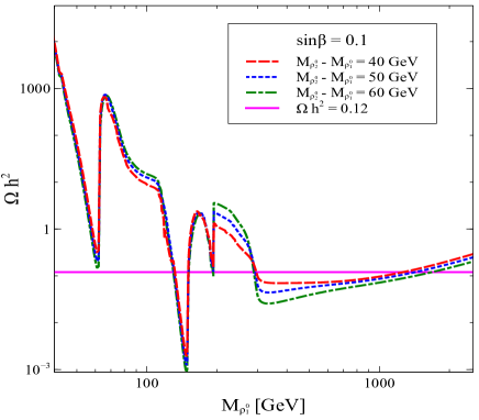
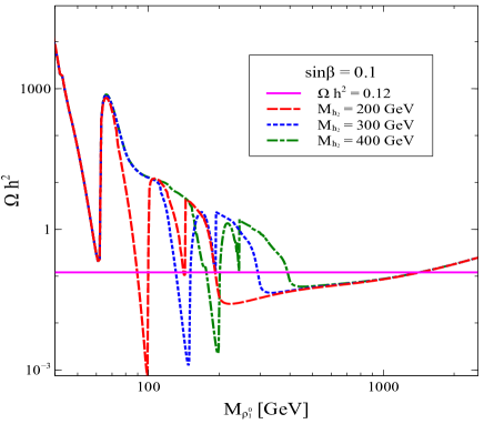
Figure 6: Left Panel: variation of DM relic density for three different value of mass difference $(M_{\rho_{2}^{0}}-M_{\rho_{1}^{0}})$ when the BSM neutral and charged Higgses values kept fixed at $M_{h_{2}}=M_{H^{\pm}}=300$ GeV. Right Panel: variation of DM relic density for three different value of the BSM Higgs mass and we kept the mass difference fixed at $M_{\rho_{2}^{0}}-M_{\rho_{1}^{0}}=$ 50 GeV. We took the other parameters value, $\sin\alpha=0.03$, $\sin\delta=0.03$.

Additionally, we also show the variation of relic density for different mass difference $\Delta M_{21}$ in the LP of Fig. 6. The first and second resonance regions show very little dependence on the mass difference $(M_{\rho_{2}^{0}}-M_{\rho_{1}^{0}})$, with the relic abundance being marginally less for higher $(M_{\rho_{2}^{0}}-M_{\rho_{1}^{0}})$. However, for the high DM mass we see that the decrease in DM relic abundance with increasing values of $(M_{\rho_{2}^{0}}-M_{\rho_{1}^{0}})$ is visible. The reason for this can be understood as follows. From Eq. (19), one can see that the singlet-triplet Yukawa coupling $Y_{\rho\Delta}$ is directly proportional to the mass difference $(M_{\rho_{2}^{0}}-M_{\rho_{1}^{0}})$. Both DM couplings $g_{\rho^{0}_{1}\rho^{0}_{1}h_{2}}$ and $g_{\rho^{0}_{1}\rho^{0}_{1}h_{1}}$ (see Eq. (22)) depend on the Yukawa coupling $Y_{\rho\Delta}$ and hence in first and second resonance regions where the s-channel processes dominate, viz., at the resonance regions mainly, controlled by resonance, hence less effect. On the other hand for higher $M_{\rho^{0}_{1}}$ regions and $t$-channel dominated regions no such resonance exists, so vary linearly with the mass differences. Close to the third resonance region, the t-channel process dominates and here, the cross-section is suppressed due to the propagator mass $M_{\rho^{\pm}}$. Therefore, for regions of the parameter space where the t-channel process dominates, the relic abundance is seen to increase as $(M_{\rho_{2}^{0}}-M_{\rho_{1}^{0}})$ (here we considered $M_{\rho^{\pm}}-M_{\rho_{2}^{0}}=160$ MeV) increases for a given $M_{\rho^{0}_{1}}$. One can see that there is clear cross over between the $t$-channel and $s$-channel diagrams for $M_{\rho_{1}^{0}}>M_{H^{\pm}},\,M_{h_{2}}$, because after this value of DM mass $\rho_{1}^{0}\rho_{1}^{0}$ mainly annihilates to $h_{2}h_{2}$ and $H^{+}H^{-}$ by the $s$-channel process mediated by the Higgses.

Finally, we also explore the dependency on the mass of the neutral Higgs $h_{2}$. In the RP of Fig. 6, we show the variation of the relic density with DM mass for three different values of the BSM Higgs mass: $M_{h_{2}}=200$ GeV, 300 GeV and 400 GeV, respectively. From the figure we see that the first resonance remains unchanged at $M_{\rho_{1}^{0}}\sim 62.5$ because the SM-like Higgs mass is fixed at $M_{h_{1}}=125.5$ GeV. However, the second resonance occurs at three different values of the DM mass depending on the values of $M_{h_{2}}$, as the resonance occurs at $M_{\rho_{1}^{0}}\sim\frac{M_{h_{2}}}{2}$. Since here we vary only the BSM Higgs mass $M_{h_{2}}$, the couplings which are related to the Higgses remain unaffected, and all three curve merge for greater values of DM mass.

To summarise, the relic density depends crucially on the mixing angles between singlet and triplet states, as well as the SM and BSM Higgs, and their masses. The BSM neutral Higgs state with mass $M_{h_{2}}$ and the charged Higgs state with suitable mass can generate multiple resonance regions, where the DM relic abundance is satisfied. The relic abundance varies inversely with the fourth power of $\sin 2\beta$ i.e., $\propto\frac{1}{\sin^{4}2\beta}$, where $\beta$ is the singlet-triplet mixing angle. The DM relic abundance is also seen to depend on the neutral Higgs mixing angle $\alpha$. Below, we discuss the correlation between different model parameters.

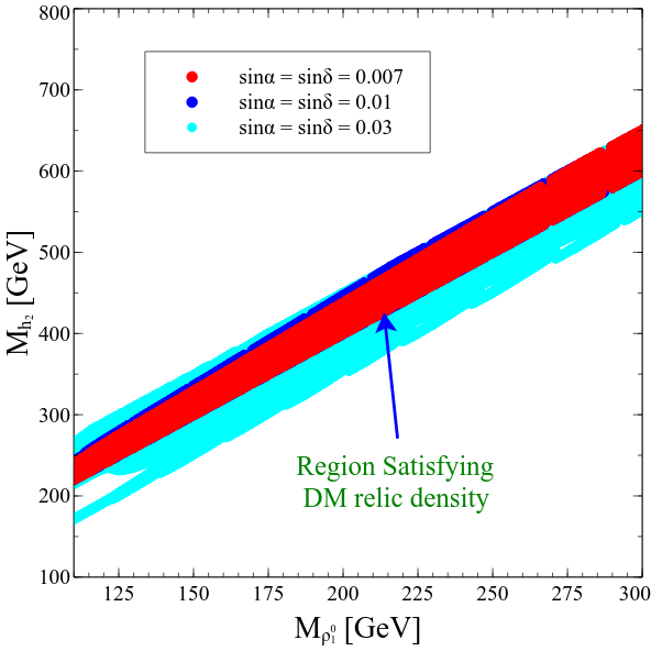
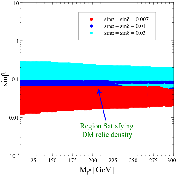
Figure 7: LP (RP): Allowed region in the $M_{\rho_{1}^{0}}-M_{h_{2}}$ ($M_{\rho_{1}^{0}}-\sin\beta$) plane after satisfying relic density bound. Other parameters values are $\Delta M_{12}=50$ GeV, $M_{H^{\pm}}=M_{h_{2}}$ and the remaining parameters have been varied as shown in Table 3.

Model Parameters	Range
$M_{\rho_{1}^{0}}$	110 - 300 [GeV]
$M_{h_{2}}$	(2 $M_{\rho_{1}^{0}}$)${}^{100}_{-50}$ [GeV]
$\sin\beta$	$10^{-3}$  -  1

Table 3: Parametsr varied in the above mentioned range at the time of generating the scatter plots.

VI Correlation between parameters

In the LP of Fig. 7 we show the allowed regions in $M_{h_{2}}$ and $M_{\rho_{1}^{0}}$, where all the dots satisfy the relic density bound as given in Eq. 1. The three colors correspond to three different benchmark choices for the Higgs mixing angle $\alpha$. From Figs. 5 and 6, one can see that the DM relic density can always be satisfied near the resonance regions. Hence, for a given BSM Higgs mass, there is only a range of DM masses that are allowed by the Planck bound. In generating the scatter plots we have varied the model parameters as shown in Table 3. We have kept the values of $M_{h_{2}}$ near the resonance region. As expected, we get a sharp correlation between the mass of DM and the BSM Higgs mass as stressed above. On the other hand, in the RP of Fig. 7 we have shown the allowed region in the sine of singlet-triplet mixing angle ($\sin\beta$) and the DM mass ($M_{\rho_{1}^{0}}$) plane. Here we keep $\Delta M_{21}=50$ GeV ($\Delta M_{21}$ as defined before), and the allowed region shows that for the given ranges as in Table 3, the DM relic density can be satisfied for $0.025<\sin\beta<0.27$. One interesting point to note here is that in the LP of Fig. 7 for $\sin\alpha$, $\sin\delta$ = 0.03, correlation in the $M_{\rho_{1}^{0}}-M_{h_{2}}$ is wider compared to the other two lower values of $\sin\alpha$, $\sin\delta$. We can understand this as follows. From the RP of Fig. 7 for $\sin\alpha$, $\sin\delta$ = 0.03, the DM relic density is satisfied for higher values of $\sin\beta$ ($\sim 0.3$). From the LP of Fig. 5 we see that near the second resonance region ($M_{\rho_{1}^{0}}\sim M_{h_{2}}/2$) the DM relic density is satisfied for a wider range of $M_{\rho^{0}_{1}}$ for higher values of $\sin\beta$. Since, for $\sin\alpha$, $\sin\delta$ = 0.03, we get higher values of $\sin\beta$ (as seen from the RP of Fig. 7), so the correlation in $M_{\rho_{1}^{0}}-M_{h_{2}}$ planes becomes wider.

The LP and RP of Fig. 8 show the allowed regions in the spin independent DD cross section and the DM mass ($\sigma_{SI}-M_{\rho_{1}^{0}}$) plane and the singlet-triplet mixing angle ($\sigma_{SI}-\sin\beta$) plane, respectively. The LP shows that the model parameter space is not constrained so-far by the results from the LUX experiment Akerib:2016vxi (and Panda experiment Cui:2017nnn ). However, a good part of the parameter space can be probed in by the Xenon 1T experiment Aprile:2017iyp and in the future by the Darwin experiment Aalbers:2016jon . The green, blue and red dots satisfy the present day relic density bound for three chosen values of $\sin\alpha$. In the RP we show the variation of the spin independent direct detection cross-section with the fermion singlet-triplet mixing angle. Since the DD cross section is directly proportional to the square of $\sin\beta$ we see this functional dependence in this figure and $\sigma_{SI}$ is seen to increase with $\sin\beta$.

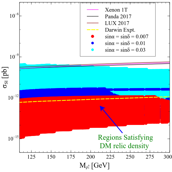
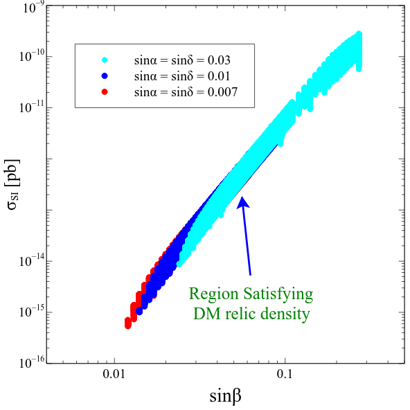
Figure 8: LP (RP): Allowed region in the $M_{\rho_{1}^{0}}-\sigma_{SI}$ ($\sin\beta-\sigma_{SI}$) plane after satisfying relic density bound. Other parameters values are $\Delta M_{12}=50$ GeV, $M_{H^{\pm}}=M_{h_{2}}$ = 300 GeV and the remaining parameters have been varied as shown in Table 3.

VII Indirect Detection of Dark Matter by $\gamma\gamma$ observation

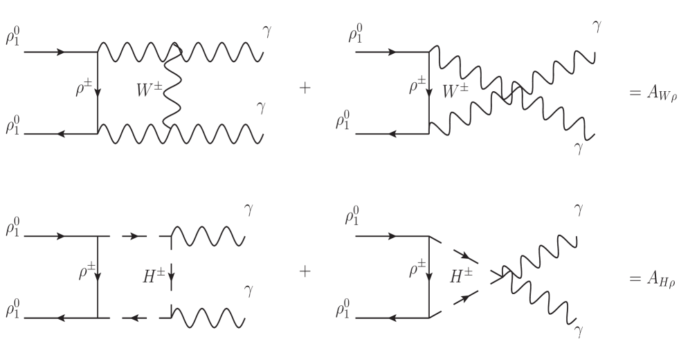
Figure 9: Feynman diagrams of the DM annihilation into the gamma rays by one loop diagrams mediated by the charge gauge boson $W^{\pm}$ and the charged scalar $H^{\pm}$.

In addition to the detection of the DM in the ongoing direct detection experiments for the present model, it can also be detected by the indirect search of DM in different satelite borne experiments like Fermi-LAT Ackermann:2013uma ; Ackermann:2015lka , HESS Abramowski:2013ax ; Profumo:2016idl by detecting the gamma-rays signal which comes from the DM annihilation. In the present situation DM cannot annihilate to gamma-rays at tree level but certainly can annihiate at the one loop level mediated by the charged gauge boson $W^{\pm}$ and the charged scalar $H^{\pm}$ which is shown in Fig. 9. The average of the amplitude for the velocity times cross section for the Feynman diagrams which are shown in Fig. 9 takes the following form Bergstrom:1997fh ; Bern:1997ng ,

$$\langle\sigma v\rangle_{\gamma\gamma}=\frac{\alpha_{EM}^{2}M^{2}_{\rho_{1}^{0}}}{16\pi^{3}}|A|^{2}$$ (29)

where $A=A_{W\rho}+A_{H\rho}$, $\alpha_{EM}=e^{2}/4\pi$ and $e=0.312$. $A_{W\rho}$ and the $A_{H\rho}$ are the separate contribution from one loop diagrams as shown in Fig. 9 which are mediated by the $W^{\pm}$ and $H^{\pm}$, respectively. The individual amplitude for the diagrams which are shown in Fig. 9 take the following form,

$$A_{W\rho} = -2C_{1}^{2}\left[2I_{3}^{a}(M_{W})+2(M_{\rho^{\pm}}^{2}+M_{W}^{2}-M_{\rho_{1}^{0}}^{2})I_{4}^{a}+2M_{\rho^{\pm}}^{2}I_{4}^{b}+3M_{\rho^{\pm}}^{2}I_{4}^{c}+I_{3}^{b}(M_{W},M_{\rho^{\pm}})\right]$$

$$+8C_{1}^{2}M_{\rho^{\pm}}M_{\rho_{1}^{0}}(I_{4}^{b}+I_{4}^{c}),$$

$$A_{H\rho} = C_{2}^{2}\left[2M_{\rho^{\pm}}^{2}I_{4}^{b}+M_{\rho^{\pm}}^{2}I_{4}^{c}+I_{3}^{b}(M_{H^{\pm}},M_{\rho_{1}^{0}})\right]$$ (30)

where the explicit form of $I_{3}^{i}$ ($i=a,b$) and $I_{4}^{j}$ ($j=a,b,c$) are given in the Appendix. The couplings $C_{1}$ and $C_{2}$ are $C_{1}=-e\sin\beta/\sin\theta_{w}$, where $\theta_{w}$ is the Weinberg angle and $C_{2}=\cos\alpha Y_{\rho\Delta}/2$, where $Y_{\rho\Delta}$ is given in Eq. (19).

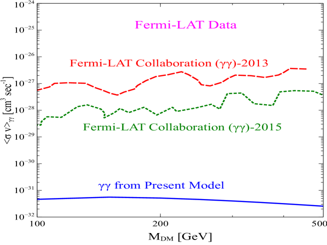
Figure 10: Fermi-LAT bounds and the prediction from the present model. In getting the prediction from the model, we have kept the parameters value fixed at $\sin\beta=0.1$, $\Delta M_{21}=50$ GeV, $M_{H^{\pm}}=M_{h_{2}}=2M_{DM}$ and $\sin\alpha=\sin\delta=0.03$.

In Fig. 10, we show the variation of $\langle\sigma v\rangle$ with the DM mass, $M_{\rho_{1}^{0}}$ by considering the relevant one loop diagrams. As the DM relic density for the pure triplet fermion is satisfied for DM mass of about $2.4$ TeV and this is already ruled out by the Fermi-LAT data when we the Sommerfeld enhancement is taken into consideration. In the current work, we have taken the triplet fermion mixing with the singlet fermion with the help of the triplet scalar and DM relic density can be satisfied around the 100 GeV order DM mass. For such low mass range of the DM where $M_{\rho_{1}^{0}}\sim M_{W}\sim M_{H^{\pm}}$, the Sommerfeld enhancement factor will have no significant role in the increment of $\langle\sigma v\rangle_{\gamma\gamma}$. We have shown the Fermi-LAT-2013 Ackermann:2013uma and Fermi-LAT-2015 Ackermann:2015lka data in the $\langle\sigma v\rangle_{\gamma\gamma}-M_{\rho_{1}^{0}}$ plane by the red and green dash line, respectively. By blue solid line we have shown the $\langle\sigma v\rangle_{\gamma\gamma}$ variation with the DM mass which is suppressed by the one loop factor for the present model.

VIII LHC Phenomenology

Although there has been no dedicated search for such a model at the LHC, one can in principle, derive limits on the masses of the exotic fermions ($\rho^{0}_{1,2}$, $\rho^{\pm}$) and the additional scalar states($h_{2}$, $H^{\pm}$) from existing LHC analyses looking for similar particles. LHC has extensively searched for heavy neutral Higgs boson similar to $h_{2}$ and the non-observation of any such states puts stringent constraints on masses and branching ratios of such particles provided their decay modes are similar to that of the SM-like Higgs Aaboud:2017gsl ; Aaboud:2017rel ; Aaboud:2017yyg . However, in our case, these bounds are significantly weakened because the decays of $h_{2}$ here are quite different compared to the conventional modes. $h_{2}$ mostly decays into $h_{1}h_{1}$, $\rho^{0}_{2}\rho^{0}_{1}$ or $\rho^{0}_{1}\rho^{0}_{1}$ pair depending on the availability of the phase space. In absence of $\rho^{0}_{2}\rho^{0}_{1}$ mode, $\rho^{0}_{1}\rho^{0}_{1}$ always has a large (30% - 40%) branching ratio, which is a completely invisible mode and thus leads to weaker event rates in the visible final states. In the presence of $\rho^{0}_{2}\rho^{0}_{1}$ and(or) $h_{1}h_{1}$ modes, a $b\bar{b}$ final state study can constrain the $h_{2}$ mass since $\rho^{0}_{2}$ always decays dominantly via $b\bar{b}$. However, the net branching ratio suppression results in weaker limits from the existing studies. Charged Higgs search at the LHC concentrates on the $\tau\bar{\nu}$, $c\bar{s}$, $c\bar{b}$ and $t\bar{b}$ decay modes depending on the mass of $H^{\pm}$ Khachatryan:2015qxa ; Khachatryan:2015uua ; CMS:2016qoa ; ATLAS:2016qiq . None of these decay modes are significant in our present scenario. Here $\rho^{\pm}$ decays via $\rho^{0}_{1}\rho^{\pm}$ and(or) $W^{\pm}Z$ depending on the particle masses. Thus the existing charged Higgs mass limits do not apply here. Instead, a dilepton or trilepton search would be more suitable for such particles although the charged leptons originating solely from the gauge boson decays will be hard to distinguish from those coming from the SM. Constraints on the masses of $\rho^{0}_{2}$ and $\rho^{\pm}$ can be drawn from searches of wino-like neutralino and chargino in the context of supersymmetry ATLAS:2017uun ; Aaboud:2017nhr . However, production cross-section of this pair at the LHC is smaller compared to the gauginos leading to weaker mass limits. Moreover, the decay pattern of $\rho^{0}_{2}$ is quite different from that of a wino-like neutralino. The most stringent gaugino mass bounds are derived from the trilepton final state analysis. Such a final state cannot be expected in our present scenario since $\rho^{0}_{2}$ dominantly decays into a $b\bar{b}$ pair along with $\rho^{0}_{1}$. However, $\rho^{\pm}$ always decays into $\rho^{0}_{1}$ associated with an on-shell or off-shell $W$-boson, similar to a wino-like chargino. Thus the bounds derived on the chargino masses in such cases ATLAS:2017uun ; Aaboud:2017nhr can be applied to $m_{\rho^{\pm}}$ as well if appropriately scaled to its production cross-section and subjected to $m_{\rho^{0}_{1}}$. We have taken this constraint into account while constructing our benchmark points.

In this section, we discuss in detail the LHC phenomenology of the dark matter. The low mass dark matter can be copiously produced at LHC, either directly or from the decay of the its triplet partner.

VIII.1 Production cross-section and choice of benchmark points

For this we consider production of $\rho^{\pm}\rho_{2}^{0}$ which further decay into $\rho_{1}^{0}$ associated with quarks resulting in a multi-jet + $\cancel{E}_{T}$ signal. Similar collider signal can also arise from other production modes, namely, $\rho_{2}^{0}\rho_{2}^{0}$ and $\rho^{+}\rho^{-}$. While the $\rho_{2}^{0}$ pair production cross-section is smaller by orders of magnitude, the other two production channels have comparable cross-sections as shown in Fig. 11.

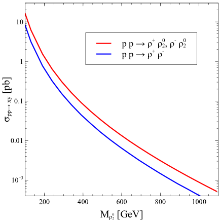
Figure 11: Variation of production cross section $\rho^{\pm}\rho_{2}^{0}$ and $\rho^{\pm}\rho^{\mp}$ with DM mass for 13 TeV run of LHC where we kept fixed $M_{\rho_{2}^{0}}-M_{\rho_{1}^{0}}=20$ GeV, $M_{h_{2}}=M_{H^{\pm}}=300$ GeV.

For Fig. 11, we have kept the mass gap between $\rho_{2}^{0}$ and $\rho_{\pm}$ fixed at the pion mass and the cross-section is computed at 13 TeV centre-of-mass energy. Clearly, $\sigma(pp\to\rho^{\pm}\rho_{2}^{0})$ is almost twice to that of $\sigma(pp\to\rho^{+}\rho^{-})$ making the former one the most favored production channel to probe for the present scenario. However, the latter one can also contribute significantly to boost the multi-jet + $\cancel{E}_{T}$ signal event rate given the fact that $\rho_{2}^{0}$ and $\rho^{\pm}$ are mass degenerate from the collider perspective. The degeneracy of $\rho_{2}^{0}$ and $\rho^{\pm}$ results in their decay products to have very similar kinematics. Therefore, in our study of the multi-jet final state we have included both the production channels $pp\to\rho_{2}^{0}\rho^{\pm}$ and $pp\to\rho^{+}\rho^{-}$. $\rho_{2}^{0}$ further decays into $\rho_{1}^{0}$ mostly via $h_{2}$ whereas $\rho^{\pm}$ also decays into $\rho_{1}^{0}$ via $W$-boson. Regardless of whether the intermediate scalar or the gauge bosons are on-shell or off-shell, we always consider their decays into pair of $b$-quarks or light quarks. In the former case, the decay of $h_{2}$ is likely to give rise to $b$-jets in the final state whereas the latter one results in light jets arising from $W$ decay. Hence in order to combine the event rates arising from these two production channels, we do not demand any $b$-tagged jets in the final states. Besides, demanding $b$-tagged jets in the final state can also hinder the signal event rates specially for cases where the mass difference between $\rho^{0}_{2}$ and $\rho^{0}_{1}$, i.e., $\Delta M_{21}$ is small.

For detail collider simulation and analysis of the above mentioned final state, we have constructed few benchmark points representative of the available parameter space after imposing all the relevant constraints. We have presented our choice of benchmark points with all the relevant particle masses and DM constraints in Table 4.

Parameters	$M_{\rho^{0}_{1}}$ [GeV]	$M_{\rho^{0}_{2}}$ [GeV]	$M_{\rho^{+}}$ [GeV]	$M_{h_{2}}$ [GeV]	$M_{H^{\pm}}$ [GeV]	$\sigma_{SI}$ [pb]	$\Omega h^{2}$
BP1	87.6	128.0	128.2	195.5	195.5	2.1 $\times 10^{-12}$	0.1207
BP2	132.0	172.0	172.2	300.0	300.0	4.1 $\times 10^{-12}$	0.1208
BP3	171.1	211.0	211.2	400.0	400.0	4.8 $\times 10^{-12}$	0.1197
BP4	86.7	200.0	200.2	194.1	194.1	1.8 $\times 10^{-11}$	0.1186
BP5	119.0	230.0	230.2	280.0	280.0	2.9 $\times 10^{-11}$	0.1195

Table 4: Benchmark points to study LHC phenomenology. We fixed other BSM parameters as $\sin\alpha=0.03$, $\sin\beta=0.1$.

Note that, the mass gap between $\rho_{2}^{0}$ (or $\rho\pm$) and $\rho_{1}^{0}$ ($\Delta M_{21}$) can not be arbitrarily large for admissible values of $\beta$. Hence in some cases, these fermionic states can lie quite close together giving rise to a compressed scenario as depicted by, for example, BP1 in Table 4. However, the mass gap can be moderate to significantly large and our choice of the benchmark points encompasses all possible kind of DM mass regions and mass hierarchies.

VIII.2 Simulation details

As mentioned previously, the mass gap $\Delta M_{21}$ can be quite small in some cases, resulting in soft jets in the final state, which may escape detection. The standard procedure is to tag the radiation jets in order to look for such scenarios. For that, one needs to take into account production of the mother particles along with additional jets and perform a proper jet-parton matching Mangano:2006rw ; Hoche:2006ph in order to avoid double counting of jets. We have considered the above mentioned production channels associated with upto two additional jets at the parton level.

$$p\,p \rightarrow XY$$

$$p\,p \rightarrow XYj$$

$$p\,p \rightarrow XYjj$$ (31)

where {X Y} indicates any of the three pairs, {$\rho_{2}^{0}$ $\rho^{+}$}, {$\rho_{2}^{0}$ $\rho^{-}$} and {$\rho^{+}$ $\rho^{-}$}. The events have been generated at the parton level using MadGraph5(v2.4.3) Alwall:2014hca ; Alwall:2011uj with CTEQ6L Pumplin:2002vw parton distribution function (PDF). Events were then passed through PYTHIA(v6.4) Sjostrand:2006za to perform showering and hadronisation effects. Matching between the shower jets and the parton level jets has been done using MLM Mangano:2006rw ; Hoche:2006ph matching scheme. We have subsequently passed the events through Delphes(v3.4.1) deFavereau:2013fsa ; Selvaggi:2014mya ; Mertens:2015kba for jet formation based on the anti-$k_{T}$ jet clustering algorithm Cacciari:2008gp via fastjet Cacciari:2011ma and for detector simulation we used the default CMS detector cuts.

Since the number of hard jets obtained in the cascade are expected to vary for the different benchmark points depending on the choice of $\Delta M_{21}$, we have chosen our final state with an optimal number of jet requirement along with missing energy: $\geq 2$-jets + ${\cancel{E}_{T}}$. The dominant SM background contributions for such a signal can arise from $QCD$, $V$+ jets, $t\bar{t}$+ jets and $VV$ + jets channels, where $V=W^{\pm}$ and $Z$. For collider analysis of this final state we have followed strategy similar to that adopted in, for example Aad:2014wea ; Dutta:2015exw .

Selection Cuts

We have used the following basic selection cuts (A0) to identify the charged leptons (e, $\mu$), photon ($\gamma$) and jets in the final state:

• Leptons are selected with $p_{T}^{l}>10$ GeV and the pseudorapidity $|\eta^{\ell}|<2.5$, where $\ell=e,\mu$.

• We used $p_{T}^{\gamma}>10$ GeV and psudorapidity $|\eta^{\gamma}|<2.5$ as the basic cuts for photon.

• We have chosen the jets which satisfy $p_{T}^{j}>40$ GeV and $|\eta^{j}|<2.5$.

• We have considered the azimuthal separation between all reconstructed jets and missing energy must be greater than 0.2 i.e. $\Delta\phi(jet,\cancel{\vec{E}}_{T})>0.2$.

In Fig. 12, we have shown the distribution function of different kinematic variable for the illustrative benchmark points after applying the basic selection cuts (A0). In addition, we also show the distribution for the SM background events. The signal event distributions shown here correspond to $\rho_{2}^{0}\rho^{\pm}$ production channel which is the dominant contributor to the final state.

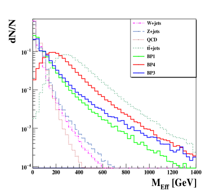
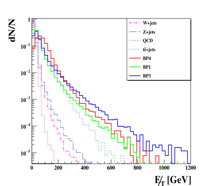
Figure 12: Normalised differential distribution with respect to the different cuts which we have used in our study. Besides the SM backgrounds we have also shown the distribution of three benchmark points BP1, BP4, BP3. All the kinematic variables have been addressed in text.

Here we have shown the distribution corresponding to the effective mass ($M_{Eff}$) and missing energy ($\cancel{E_{T}}$) where the effective mass defined in the following way,

$$M_{Eff}=\sum_{i}|\vec{p}_{T_{i}}^{j}|+\sum_{i}|\vec{p}_{T_{i}}^{\ell}|+\cancel{E_{T}}$$ (32)

These distributionis show some distinguishing features of the signal events from the SM backgrounds. Guided by these distributions we now proceed to device some appropriate kinematic cuts to optimise the signal to background events ratio in order to maximise the statistical significance of the signal.

1. Since we are studying a hadronic final state, we have imposed a lepton and photon veto in the final state. This cut coupled with a large ${\cancel{E}_{T}}$ cut helps to reduce background events particularly arising from $W$ + jets when $W$ decays leptonically.

2. $p_{T}$ requirements on the hardest and second hardest jets: $p_{T}^{j_{1}}>130$ GeV and $p_{T}^{j_{2}}>80$ GeV. This cut significantly reduce the V + jets (where V = $W^{\pm}$, Z) and QCD backgrounds.

3. The $QCD$ multi-jet events have no direct source of missing energy. Therefore, any contribution to ${\cancel{E}_{T}}$ in these events must arise from the mismeasurement of the jet $p_{T}$s. In order to minimise this effect, we have ensured that the $\cancel{\vec{E}}_{T}$ and the jets are well separated, i.e., $\Delta\phi(j_{i},\cancel{\vec{E}}_{T})>0.4$ where i = 1, 2. For all the other jets, $\Delta\phi(j,\cancel{\vec{E}}_{T})>0.2$.

4. We demand a hard cut on the effective mass variable, $M_{Eff}>800$ GeV.

5. We put the bound on the missing enrgy $\cancel{E}_{T}>160$ GeV.

   $M_{Eff}$ and $\cancel{E_{T}}$ are the two most effective cuts to reduce SM background events for multi-jet analyses. As shown in Fig. 12, these variables clearly separates the signal kinematical region from most of the dominant backgrounds quite effectively and can reduce the backgrounds in a significant amount. Most importantly, these cuts along with A1 and A2, reduces the large $QCD$ background to a neglible amount.

Results

In Table 5 and 6, we have shown numerical results of our collider analysis in production channels $\rho_{2}^{0}\rho^{\pm}$ and $\rho^{+}\rho^{-}$ respectively corresponding to the five choosen benchmark points (as shown in Table 4) which satisfy the present day accepted value of the DM relic density and are safe from the different ongoing direct detection experiment. We have studied the SM background in detail and in Table 7 we have shown the resulting cross sections after appyling the aforementioned cuts. Here, we have considered NLO cross section for all the SM background processes as provided in Alwall:2014hca .

Signal at 13 TeV BP Cross-section (pb) BP1 6.757 BP2 2.279 BP3 1.052 BP4 1.296 BP5 0.760

Effective Cross section after applying cuts (fb) A0 + A1    A2    A3    A4    A5 1005.05 175.08 138.45 22.02 19.15 385.22 69.16 56.51 11.87 10.85 189.71 34.63 29.19 7.36 6.82 1047.86 145.67 116.94 14.19 9.82 616.00 89.60 72.63 9.80 7.40

Table 5: Cut-flow table for the obtained signal cross section at 13 TeV LHC corresponding to $\rho^{0}_{2}\rho^{\pm}$ channel. The five benchmark points are referred as BP1-BP5. See the text for the details of the cuts A0-A5.

Signal at 13 TeV BP Cross-section (pb) BP1 3.419 BP2 1.156 BP3 0.532 BP4 0.652 BP5 0.380

Effective Cross section after applying cuts (fb) A0 + A1    A2    A3    A4    A5 2639.30 74.36 59.18 8.54 7.31 880.60 28.77 23.87 4.95 4.43 402.24 14.80 12.62 3.18 2.95 446.80 63.99 45.54 5.72 3.76 258.55 34.40 28.07 3.99 3.08

Table 6: Cut-flow table for the obtained signal cross section at 13 TeV LHC corresponding to $\rho^{+}\rho^{-}$ channel. The five benchmark points are referred as BP1-BP5. See the text for the details of the cuts A0-A5.

SM Backgrounds at 13 TeV Channels Cross-section (pb) Z $+\leq$ 4 jets 5.7$\times 10^{4}$ W± + $\leq$ 4 jets 1.9$\times 10^{5}$ QCD ($\leq$ 4 jets) 2.0$\times 10^{8}$ t $\bar{\rm t}+$ $\leq$ 2 jets 722.94 W±Z + $\leq$ 2 jets 51.10 Z Z +$\leq$ 2 jets 13.71 Total Backgrounds

Effective Cross section after applying cuts (pb) A0 + A1    A2    A3    A4    A5 5.5 $\times 10^{3}$ 361.90 241.60 11.40 2.20 9.1 $\times 10^{3}$ 783.20 504.00 18.90 1.50 1.5 $\times 10^{7}$ 3.5 $\times 10^{5}$ 2.4 $\times 10^{5}$ 2.5 $\times 10^{3}$ - 493.73 171.46 120.63 13.89 1.94 19.66 5.37 3.59 0.50 0.12 4.99 0.80 0.53 0.06 0.02 5.78

Table 7: Cut-flow table for the obtained cross-sections corresponding to the relevant SM background channels for the cuts A0-A5 as mentioned in the text at the LHC with 13 TeV center-of-mass energy.

In order to compute statistical significance ($\mathcal{S}$) of our signal for the different benchmark points over the SM background we have used

$$\mathcal{S}=\sqrt{2\times\left[(s+b)\,{\rm ln}\left(1+\frac{s}{b}\right)-s\right]}.$$ (33)

where $s$ is the number of signal events and $b$ that of the total SM background contribution. In Table 8, we have shown the statistical significance obtained for 100 ${\rm fb}^{-1}$ integrated luminosity ($\mathcal{L}$). In the last column we have also shown the required ${\mathcal{L}}$ to achieve $3\sigma$ statistical significance for our benchmark points at 13 TeV LHC.

Signal at 13 TeV BP DM mass [GeV] BP1 87.6 BP2 132.0 BP3 171.1 BP4 86.7 BP5 119.0

Statitical Significance ($\mathcal{S}$) $\mathcal{L}=100$ ${\rm fb^{-1}}$ 3.5 2.0 1.3 1.8 1.4

Required Luminosity $\mathcal{L}$ (${\rm fb^{-1}}$) $\mathcal{S}=3\sigma$ 74.4 223.0 545.3 282.3 473.9

Table 8: Statistical significance of the multi-jet signal corresponding to different benchmark points for ${\mathcal{L}}=100\leavevmode\nobreak\ {\rm fb}^{-1}$ integrated luminosity along with the required luminosity to achieve $3\sigma$ statistical significance at 13 TeV run of the LHC.

As evident from Table 5, 6, 7 and 8, the used kinematical cuts are efficient enough to reduce the SM background contributions to the multi-jet channel. At the same time sufficient number of signal events survive leading to discovery potential of such a scenario at the 13 TeV run of the LHC with realistic integrated luminosities. The cuts A2, A4 and A5 are particularly useful in reducing the dominant background constributions arising from $W$ + jets, $Z$ + jets and $t\bar{t}$ + jets. A combination of cuts A2-A5 has reduced the QCD contribution to a negligible amount. As the numbers indicate in Table 8, BP1 can be probed at the 13 TeV run of the LHC with 3$\sigma$ statistical significance with relatively low luminosity owing to the large production cross-section. As expected, the signal significance declines as the mass of $\rho_{2}^{0}$ ($\rho^{\pm}$) is increased while its mass gap with $\rho_{1}^{0}$ is kept same as represented by the numbers corresponding to the two subsequent benchmark points (BP2 and BP3). The last two benchmark points, BP4 and BP5 represent the scenario when the parent particles have masses significantly higher than the DM candidate. As a result, one would expect the cut efficiencies to improve for these benchmark points. This is reflected for example in the case of BP5 which has a signal significance very similar to BP3 in spite of having the smallest production cross-section. It can be inferred from our analysis that $\rho_{2}^{0}$ ($\rho^{\pm}$) masses $\sim$ 250 GeV can easily be probed at the 13 TeV LHC with a reasonable luminosity.

IX Conclusion and Summary

For the WIMP-type DM, its relic density, detection at direct detection experiments, and detection at collider experiments are intimately inter-related. In this work we have proposed a fermion DM model that can successfully explain the DM relic density, can be tested in future direct detection experiments, and can be produced and tested at the 13 TeV run of the LHC.

The model we propose extends the SM particle content by a SM triplet fermion and a SM singlet fermion, as well as by a SM triplet scalar. Both new fermions are given Majorana masses. An overall discrete $\mathbb{Z}_{2}$ symmetry is imposed and the corresponding charges of the particles under this symmetry is arranged in such as way that the only Yukawa coupling involving the new fermions is the one which includes the triplet fermion, the singlet fermion and the triplet scalar. This gives rise to the mixing between the neutral component of the SM triplet fermion mixing with the SM singlet fermion. The lighter of the two mass eigenstates becomes the DM candidate in the model, stabilised by the $\mathbb{Z}_{2}$ symmetry. There is also mixing between the neutral as well as charged scalar degrees of freedom belonging to the SM doublet and triplet representations. Finally, we get two physical neutral scalars - one SM-like Higgs $h_{1}$ of mass 125.5 GeV and another heavier BSM Higgs $h_{2}$ whose mass we keep as a free parameter in the model. From the charged scalar sector, we get physical charged scalars $H^{\pm}$ while the other degree of freedom becomes the charged Goldstone boson, which is ‘eaten up’ to give mass to the $W^{\pm}$ bosons. The presence of the triplet scalar as well as the mixing between the triplet and singlet fermions lead to additional $s$-channel diagrams mediated by $h_{1}$ and $h_{2}$ as well as $t$-channel diagrams mediated by the new fermions $\rho^{0}_{1,2}$ and $\rho^{\pm}$ with $H^{\pm}$ or $h_{2}$ in their final states. These additional diagrams allow for resonant production of DM at (1) $h_{1}$ mediated $s$-channel processes, (2) $h_{2}$ mediated $s$-channel processes, and (3) $t$-channel diagrams with $H^{\pm}$ or $h_{2}$ in their final states. This allows us to satisfy the observed DM relic density by Planck with DM masses in the 100 GeV range. We study the impact of the model parameters on the DM relic density. We also study the possibility of testing this model at the current and future direct detection experiments, Xenon 1T and Darwin.

Finally we study the LHC phenomenology for few benchmark points (BP) and show that this model is testable in the very near future run of LHC. The model proposed in Ma:2008cu had only the triplet fermion (and an inert doublet scalar) where the neutral component of the triplet becomes the DM stabilised by the $\mathbb{Z}_{2}$ symmetry. The relic density of the fermionic DM in that model was governed by the $t$-channel processes involving only the $W^{\pm}$, SM-like Higgs and SM fermions. As a result, the DM mass was seen to be 2.37 TeV for the Planck bound to be satisfied. Hence, this model cannot be tested at the LHC. Since the DM mass in our model is ${\cal O}(100$ GeV), therefore, we can produce them in the collider at the 13 TeV run of LHC with a reasonably large cross-section. In this work we analysed the multi jets + missing energy signal. We also considered the low mass difference between the DM ($\rho_{1}^{0}$) and the next-to-lightest neutral particle ($\rho_{2}^{0}$), that might lead to softer jets. However, high $p_{T}$ jets may come from the ISR. Corresponding to this signal we figured out the dominant SM backgrounds for multi jets + missing energy signal. By suitably choosing the cuts we have reduced the SM backgrounds and simultaneously increased the statistical significance of the signal. We showed that for 100 fb^-1, we could observe the DM with $3.5\sigma$ statistical significance for one of the BP. The statistical significance was seen reduce as the mass of $\rho^{0}_{2}$ and $\rho^{\pm}$ was increased. We also studied how much luminosity would be required to probe this model with a $3\sigma$ statistical significance for our BPs.

A final comment on our model is in order. While we have focussed only on explaining the DM relic density within the context of the present model, we can easily extend it to generate the neutrino masses by Type I seesaw mechanism. This can be done by introducing right-handed neutrinos.

In conclusion, the present model allows for low mass fermionic DM that satisfactorily produces the observed the relic density of the universe. It can be tested at the current and next-generation DM direct detection experiments. More importantly the 100 GeV mass range of the DM candidate in this model allows its production and detection at the LHC. The 13 TeV LHC can discover this fermionic DM candidate for with more than $3\sigma$ statistical significance with reasonable luminosity.

Appendix

The factors $I_{4}^{j}$ and $I_{3}^{i}$ take the following form Bergstrom:1997fh ; Bern:1997ng , as used in the Eq. (30), for the $A_{W\rho}$ part $I_{4}^{j}$ has the following structure,

$$I_{4}^{a} = \frac{I_{3}^{2}(M_{W},M_{\rho^{\pm}})I_{2}^{1}(M_{W})}{M_{\rho_{1}^{0}}^{2}+M_{\rho^{\pm}}^{2}-M_{W}^{2}},$$

$$I_{4}^{b} = \frac{I_{3}^{2}(M_{\rho^{\pm}},M_{W})-I_{3}^{1}(M_{\rho^{\pm}})}{M_{\rho_{1}^{0}}^{2}-M_{\rho^{\pm}}^{2}+M_{W}^{2}},$$

$$I_{4}^{c} = \frac{I_{3}^{2}(M_{\rho^{\pm}},M_{W})-I_{3}^{2}(M_{W},M_{\rho^{\pm}})}{M_{\rho^{\pm}}^{2}-M_{W}^{2}}$$ (34)

and for determing the amplitude $A_{H\rho}$, we just need to replace the $W^{\pm}$ gauge boson mass ($M_{W}$) by the mass ($M_{H^{\pm}}$) of the charged scalar $H^{\pm}$. Now the $I_{3}^{i}$ components take the following form,

$$I_{3}^{a}(m)=\Bigg{\{}\begin{matrix}\frac{1}{8\,M^{2}_{\rho_{1}^{0}}}[\log^{2}(\frac{1+x}{1-x})-\pi^{2}-2i\pi\log(\frac{1+x}{1-x})],&m\leq M_{\rho_{1}^{0}}\\ -\frac{1}{2M_{\rho_{1}^{0}}^{2}}\left(\tan^{-1}(\frac{1}{m^{2}/M_{\rho_{1}^{0}}^{2}}-1)\right),&m>M_{\rho_{1}^{0}}\end{matrix}$$ (35)

and the other component takes the form,

$$I_{3}^{b}(m_{1},m_{2}) = \frac{1}{2M_{\rho_{1}^{0}}^{2}}\left[Li_{2}\left(\frac{m_{1}^{2}-M_{\rho_{1}^{0}}^{2}-m_{2}^{2}-\sqrt{\Delta_{1}}}{2m_{1}^{2}}\right)+Li_{2}\left(\frac{m_{1}^{2}-M_{\rho_{1}^{0}}^{2}-m_{2}^{2}+\sqrt{\Delta_{1}}}{2m_{1}^{2}}\right)\right]$$

$$-\frac{1}{2M_{\rho_{1}^{0}}^{2}}\left[Li_{2}\left(\frac{m_{1}^{2}+M_{\rho_{1}^{0}}^{2}-m_{2}^{2}-\sqrt{\Delta_{2}}}{2m_{1}^{2}}\right)+Li_{2}\left(\frac{m_{1}^{2}+M_{\rho_{1}^{0}}^{2}-m_{2}^{2}+\sqrt{\Delta_{2}}}{2m_{1}^{2}}\right)\right]$$

where

$$x = \sqrt{1-m^{2}/M_{\rho_{1}^{0}}}$$

$$\Delta_{1} = (m_{1}^{2}+M_{\rho_{1}^{0}}^{2}-m_{2}^{2})^{2}+4M_{\rho_{1}^{0}}^{2}m_{2}^{2}$$

$$\Delta_{1} = (m_{1}^{2}-M_{\rho_{1}^{0}}^{2}-m_{2}^{2})^{2}-4M_{\rho_{1}^{0}}^{2}m_{2}^{2}$$

References

- (1) Y. Sofue and V. Rubin, “Rotation curves of spiral galaxies”, Ann. Rev. Astron. Astrophys. 39, 137 (2001) [astro-ph/0010594].
- (2) M. Bartelmann and P. Schneider, “Weak gravitational lensing”, Phys. Rept. 340, 291 (2001) [astro-ph/9912508].
- (3) D. Clowe, A. Gonzalez and M. Markevitch, “Weak lensing mass reconstruction of the interacting cluster 1E0657-558: Direct evidence for the existence of dark matter”, Astrophys. J. 604, 596 (2004) [astro-ph/0312273].
- (4) D. Harvey, R. Massey, T. Kitching, A. Taylor and E. Tittley, “The non-gravitational interactions of dark matter in colliding galaxy clusters”, Science 347, 1462 (2015) [arXiv:1503.07675 [astro-ph.CO]].
- (5) G. Hinshaw et al. [WMAP Collaboration], “Nine-Year Wilkinson Microwave Anisotropy Probe (WMAP) Observations: Cosmological Parameter Results”, Astrophys. J. Suppl. 208, 19 (2013) [arXiv:1212.5226 [astro-ph.CO]].
- (6) P. A. R. Ade et al. [Planck Collaboration], “Planck 2015 results. XIII. Cosmological parameters”, arXiv:1502.01589 [astro-ph.CO].
- (7) J. Hisano, S. Matsumoto and M. M. Nojiri, “Unitarity and higher order corrections in neutralino dark matter annihilation into two photons”, Phys. Rev. D 67, 075014 (2003) [hep-ph/0212022].
- (8) J. Hisano, S. Matsumoto and M. M. Nojiri, “Explosive dark matter annihilation”, Phys. Rev. Lett. 92, 031303 (2004) [hep-ph/0307216].
- (9) J. Hisano, S. Matsumoto, M. M. Nojiri and O. Saito, “Non-perturbative effect on dark matter annihilation and gamma ray signature from galactic center”, Phys. Rev. D 71, 063528 (2005) [hep-ph/0412403].
- (10) M. Cirelli, N. Fornengo and A. Strumia, “Minimal dark matter”, Nucl. Phys. B 753, 178 (2006) [hep-ph/0512090].
- (11) J. Hisano, S. Matsumoto, M. Nagai, O. Saito and M. Senami, “Non-perturbative effect on thermal relic abundance of dark matter”, Phys. Lett. B 646, 34 (2007) [hep-ph/0610249].
- (12) E. Ma and D. Suematsu, “Fermion Triplet Dark Matter and Radiative Neutrino Mass”, Mod. Phys. Lett. A 24, 583 (2009) [arXiv:0809.0942 [hep-ph]].
- (13) T. Cohen, M. Lisanti, A. Pierce and T. R. Slatyer, “Wino Dark Matter Under Siege”, JCAP 1310, 061 (2013) [arXiv:1307.4082 [hep-ph]].
- (14) P. Chardonnet, P. Salati and P. Fayet, “Heavy triplet neutrinos as a new dark matter option”, Nucl. Phys. B 394, 35 (1993).
- (15) C. Biggio and F. Bonnet, “Implementation of the Type III Seesaw Model in FeynRules/MadGraph and Prospects for Discovery with Early LHC Data”, Eur. Phys. J. C 72, 1899 (2012) [arXiv:1107.3463 [hep-ph]].
- (16) M. Hirsch, R. A. Lineros, S. Morisi, J. Palacio, N. Rojas and J. W. F. Valle, “WIMP dark matter as radiative neutrino mass messenger”, JHEP 1310, 149 (2013) [arXiv:1307.8134 [hep-ph]].
- (17) A. Chaudhuri, N. Khan, B. Mukhopadhyaya and S. Rakshit, Phys. Rev. D 91, 055024 (2015) doi:10.1103/PhysRevD.91.055024 [arXiv:1501.05885 [hep-ph]].
- (18) S. Bhattacharya, N. Sahoo and N. Sahu, “Singlet-Doublet Fermionic Dark Matter, Neutrino Mass and Collider Signatures”, Phys. Rev. D 96, no. 3, 035010 (2017) [arXiv:1704.03417 [hep-ph]].
- (19) M. Frigerio and T. Hambye, “Dark matter stability and unification without supersymmetry”, Phys. Rev. D 81, 075002 (2010) [arXiv:0912.1545 [hep-ph]].
- (20) Y. Mambrini, N. Nagata, K. A. Olive and J. Zheng, “Vacuum Stability and Radiative Electroweak Symmetry Breaking in an SO(10) Dark Matter Model”, Phys. Rev. D 93, no. 11, 111703 (2016) [arXiv:1602.05583 [hep-ph]].
- (21) J. Erler and P. Langacker, “Electroweak model and constraints on new physics”, hep-ph/0407097.
- (22) J. Erler and P. Langacker, “Electroweak Physics”, Acta Phys. Polon. B 39, 2595 (2008) [arXiv:0807.3023 [hep-ph]].
- (23) M. C. Chen, S. Dawson and C. B. Jackson, “Higgs Triplets, Decoupling, and Precision Measurements”, Phys. Rev. D 78, 093001 (2008) [arXiv:0809.4185 [hep-ph]].
- (24) A. Abada, C. Biggio, F. Bonnet, M. B. Gavela and T. Hambye, “ e and tau —¿ l gamma decays in the fermion triplet seesaw model”, Phys. Rev. D 78, 033007 (2008) [arXiv:0803.0481 [hep-ph]].
- (25) G. Belanger, F. Boudjema, A. Pukhov and A. Semenov, “Dark matter direct detection rate in a generic model with micrOMEGAs 2.2”, Comput. Phys. Commun. 180, 747 (2009) [arXiv:0803.2360 [hep-ph]].
- (26) D. S. Akerib et al. [LUX Collaboration], “Improved Limits on Scattering of Weakly Interacting Massive Particles from Reanalysis of 2013 LUX Data”, Phys. Rev. Lett. 116, no. 16, 161301 (2016) [arXiv:1512.03506 [astro-ph.CO]].
- (27) D. S. Akerib et al. [LUX Collaboration], “Results from a search for dark matter in the complete LUX exposure”, Phys. Rev. Lett. 118, no. 2, 021303 (2017) [arXiv:1608.07648 [astro-ph.CO]].
- (28) E. Aprile et al. [XENON Collaboration], “Physics reach of the XENON1T dark matter experiment”, JCAP 1604, no. 04, 027 (2016) [arXiv:1512.07501 [physics.ins-det]].
- (29) E. Aprile et al. [XENON Collaboration], “First Dark Matter Search Results from the XENON1T Experiment”, arXiv:1705.06655 [astro-ph.CO].
- (30) X. Cui et al. [PandaX-II Collaboration], “Dark Matter Results From 54-Ton-Day Exposure of PandaX-II Experiment”, arXiv:1708.06917 [astro-ph.CO].
- (31) J. Aalbers et al. [DARWIN Collaboration], “DARWIN: towards the ultimate dark matter detector”, JCAP 1611, 017 (2016) [arXiv:1606.07001 [astro-ph.IM]].
- (32) A. Abramowski et al. [H.E.S.S. Collaboration], “Search for Photon-Linelike Signatures from Dark Matter Annihilations with H.E.S.S.”, Phys. Rev. Lett. 110, 041301 (2013) [arXiv:1301.1173 [astro-ph.HE]].
- (33) S. Profumo, F. S. Queiroz and C. E. Yaguna, “Extending Fermi-LAT and H.E.S.S. Limits on Gamma-ray Lines from Dark Matter Annihilation”, Mon. Not. Roy. Astron. Soc. 461, no. 4, 3976 (2016) [arXiv:1602.08501 [astro-ph.HE]].
- (34) M. Ackermann et al. [Fermi-LAT Collaboration], “Search for Gamma-ray Spectral Lines with the Fermi Large Area Telescope and Dark Matter Implications”, Phys. Rev. D 88, 082002 (2013) [arXiv:1305.5597 [astro-ph.HE]].
- (35) M. Ackermann et al. [Fermi-LAT Collaboration], “Updated search for spectral lines from Galactic dark matter interactions with pass 8 data from the Fermi Large Area Telescope”, Phys. Rev. D 91, no. 12, 122002 (2015) [arXiv:1506.00013 [astro-ph.HE]].
- (36) L. Bergstrom and P. Ullio, “Full one loop calculation of neutralino annihilation into two photons”, Nucl. Phys. B 504, 27 (1997) [hep-ph/9706232].
- (37) Z. Bern, P. Gondolo and M. Perelstein, “Neutralino annihilation into two photons”, Phys. Lett. B 411, 86 (1997) [hep-ph/9706538].
- (38) G. Aad et al. [ATLAS and CMS Collaborations], “Measurements of the Higgs boson production and decay rates and constraints on its couplings from a combined ATLAS and CMS analysis of the LHC pp collision data at and 8 TeV”, JHEP 1608, 045 (2016) [arXiv:1606.02266 [hep-ex]].
- (39) A. Alloul, N. D. Christensen, C. Degrande, C. Duhr and B. Fuks, “FeynRules 2.0 - A complete toolbox for tree-level phenomenology”, Comput. Phys. Commun. 185, 2250 (2014) [arXiv:1310.1921 [hep-ph]].
- (40) G. Belanger, F. Boudjema, A. Pukhov and A. Semenov, “micrOMEGAs-3: A program for calculating dark matter observables”, Comput. Phys. Commun. 185, 960 (2014) [arXiv:1305.0237 [hep-ph]].
- (41) D. S. M. Alves, E. Izaguirre and J. G. Wacker, “It’s On: Early Interpretations of ATLAS Results in Jets and Missing Energy Searches”, Phys. Lett. B 702, 64 (2011) [arXiv:1008.0407 [hep-ph]].
- (42) M. Aaboud et al. [ATLAS Collaboration], “Search for heavy resonances decaying into in the final state in collisions at TeV with the ATLAS detector”, Eur. Phys. J. C 78, no. 1, 24 (2018) [arXiv:1710.01123 [hep-ex]].
- (43) M. Aaboud et al. [ATLAS Collaboration], “Search for heavy resonances in the and final states using proton proton collisions at TeV with the ATLAS detector”, arXiv:1712.06386 [hep-ex].
- (44) M. Aaboud et al. [ATLAS Collaboration], “Search for new phenomena in high-mass diphoton final states using 37 fb-1 of proton–proton collisions collected at TeV with the ATLAS detector”, Phys. Lett. B 775, 105 (2017) [arXiv:1707.04147 [hep-ex]].
- (45) V. Khachatryan et al. [CMS Collaboration], “Search for a charged Higgs boson in pp collisions at TeV”, JHEP 1511, 018 (2015) [arXiv:1508.07774 [hep-ex]].
- (46) V. Khachatryan et al. [CMS Collaboration], “Search for a light charged Higgs boson decaying to in pp collisions at TeV”, JHEP 1512, 178 (2015) [arXiv:1510.04252 [hep-ex]].
- (47) CMS Collaboration [CMS Collaboration], “Search for Charged Higgs boson to in lepton+jets channel using top quark pair events”, CMS-PAS-HIG-16-030.
- (48) The ATLAS collaboration [ATLAS Collaboration], “Search for charged Higgs bosons in the decay channel in collisions at TeV using the ATLAS detector”, ATLAS-CONF-2016-089.
- (49) The ATLAS collaboration [ATLAS Collaboration], “Search for electroweak production of supersymmetric particles in the two and three lepton final state at TeV with the ATLAS detector”, ATLAS-CONF-2017-039.
- (50) M. Aaboud et al. [ATLAS Collaboration], “Search for the direct production of charginos and neutralinos in final states with tau leptons in 13 TeV collisions with the ATLAS detector”, Eur. Phys. J C 78, 154 (2018) [arXiv:1708.07875 [hep-ex]].
- (51) M. L. Mangano, M. Moretti, F. Piccinini and M. Treccani, “Matching matrix elements and shower evolution for top-quark production in hadronic collisions”, JHEP 0701, 013 (2007) [hep-ph/0611129].
- (52) S. Hoeche, F. Krauss, N. Lavesson, L. Lonnblad, M. Mangano, A. Schalicke and S. Schumann, “Matching parton showers and matrix elements”, hep-ph/0602031.
- (53) J. Alwall et al., “The automated computation of tree-level and next-to-leading order differential cross sections, and their matching to parton shower simulations”, JHEP 1407, 079 (2014) [arXiv:1405.0301 [hep-ph]].
- (54) J. Alwall, M. Herquet, F. Maltoni, O. Mattelaer and T. Stelzer, “MadGraph 5 : Going Beyond”, JHEP 1106, 128 (2011) [arXiv:1106.0522 [hep-ph]].
- (55) J. Pumplin, D. R. Stump, J. Huston, H. L. Lai, P. M. Nadolsky and W. K. Tung, “New generation of parton distributions with uncertainties from global QCD analysis”, JHEP 0207, 012 (2002) [hep-ph/0201195].
- (56) T. Sjostrand, S. Mrenna and P. Z. Skands, “PYTHIA 6.4 Physics and Manual”, JHEP 0605, 026 (2006) [hep-ph/0603175].
- (57) J. de Favereau et al. [DELPHES 3 Collaboration], “DELPHES 3, A modular framework for fast simulation of a generic collider experiment”, JHEP 1402, 057 (2014) [arXiv:1307.6346 [hep-ex]].
- (58) M. Selvaggi, “DELPHES 3: A modular framework for fast-simulation of generic collider experiments”, J. Phys. Conf. Ser. 523, 012033 (2014).
- (59) A. Mertens, “New features in Delphes 3”, J. Phys. Conf. Ser. 608, no. 1, 012045 (2015).
- (60) M. Cacciari, G. P. Salam and G. Soyez, “The Anti-k(t) jet clustering algorithm”, JHEP 0804, 063 (2008) [arXiv:0802.1189 [hep-ph]].
- (61) M. Cacciari, G. P. Salam and G. Soyez, “FastJet User Manual”, Eur. Phys. J. C 72, 1896 (2012) [arXiv:1111.6097 [hep-ph]].
- (62) G. Aad et al. [ATLAS Collaboration], “Search for squarks and gluinos with the ATLAS detector in final states with jets and missing transverse momentum using TeV proton–proton collision data”, JHEP 1409, 176 (2014) [arXiv:1405.7875 [hep-ex]].
- (63) J. Dutta, P. Konar, S. Mondal, B. Mukhopadhyaya and S. K. Rai, “A Revisit to a Compressed Supersymmetric Spectrum with 125 GeV Higgs”, JHEP 1601, 051 (2016) [arXiv:1511.09284 [hep-ph]].