Universal quantum computation with temporal-mode bilayer square lattices

We propose an experimental design for universal continuous-variable quantum computation that incorporates recent innovations in linear-optics-based continuous-variable cluster state generation and cubic-phase gate teleportation. The first ingredient is a protocol for generating the bilayer-square-lattice cluster state (a universal resource state) with temporal modes of light. With this state, measurement-based implementation of Gaussian unitary gates requires only homodyne detection. Second, we describe a measurement device that implements an adaptive cubic-phase gate, up to a random phase-space displacement. It requires a two-step sequence of homodyne measurements and consumes a (non-Gaussian) cubic-phase state.

I Introduction

Recently, there has been substantial progress in developing the basic building blocks of quantum computation using continuous-variable cluster states (CVCSs) Menicucci2006 . Two-dimensional (or higher-dimensional) cluster states enable universal quantum computation provided that one can also perform suitable sequences of single-site measurements Raussendorf2001 ; Menicucci2006 . Thus, much effort has focused on generating large-scale cluster states and implementing sets of measurements that enable universal measurement-based quantum computation (MBQC) Gu2009 .

The scalability of one-dimensional CVCS architectures is now well established. Recent experimental demonstrations have yielded states consisting of 60 frequency modes (where each mode is simultaneously addressable) Chen2014 and greater than one million temporal modes (where each mode is sequentially addressable) with no significant experimental obstacles hindering the generation of even larger states Yokoyama2013 ; Yoshikawa2016 . These states are endowed with a multi-layered graph , from which can be derived a simple and compact state generation circuit consisting of offline squeezers and constant-depth linear optics Menicucci2011a . This feature makes them highly compatible with multi-mode squeezing platforms, such as optical parametric oscillators (OPOs) Menicucci2007 ; Menicucci2008 ; Flammia2009 ; Menicucci2011a and Josephson traveling-wave parametric amplifiers Grimsmo2017 . Though these states generalize to two Alexander2016b ; Menicucci2011a ; Wang2014 and higher dimensions Wang2014 , the generation of such a scalable universal cluster state has yet to be demonstrated.

Complementary to this work is an effort to implement a universal set of continuous-variable gates using tailored small-scale resource states (prepared offline) and gate teleportation Lloyd1999 . Examples include demonstrations of single-mode Gaussian operations (including linear optics and squeezing) Filip2005 ; Yoshikawa2007 ; Yoshikawa2011 , single-mode non-Gaussian operations such as the cubic-phase gate Yukawa2013 ; Yukawa2013a ; Marshall2015a ; Miyata2016 ; Arzani2017 , and the two-mode sum gate Yoshikawa2008 . Such demonstrations are gate-specific and have remained limited to small-scale implementations. It is therefore desirable to synthesize these elements into one universal, scalable design.

Here we consider an approach to universal quantum computation that seeks to marry the above research threads. We begin by modifying an existing protocol (proposed by some of us) for generating a universal cluster state known as the bilayer square lattice Alexander2016b (BSL). Our implementation makes use of temporal modes, and requires four squeezers, five beamsplitters, and two delay loops. The practicality of this scheme stems from its similarity to the aforementioned one-dimensional experiment Yoshikawa2016 .

Beyond state generation, much of the previous work on quantum computing with CVCSs has focused on Gaussian operations Ukai2010 ; Ukai2011 ; Su2013 ; Miyata2014 ; Ferrini2013a ; Alexander2014 ; Yokoyama2015 ; Ferrini2016 ; Alexander2016 , which can be implemented with non-adaptive homodyne measurements Menicucci2006 ; Gu2009 and can be efficiently simulated Bartlett2002 . Universal quantum computation requires non-Gaussian gates, which can be implemented by measuring quadratic or higher order polynomials in the quadrature operators or by injecting non-Gaussian single-mode states directly into the cluster state Gu2009 . In order for non-Gaussian computations to proceed deterministically, the measurements must be adaptive Gu2009 .

Other than the present proposal, Ref. Gu2009 is the only explicit experimental proposal for implementing a universal set of measurement-based gates on a CVCS. In that approach, a non-Gaussian gate known as the cubic-phase gate is implemented on a CVCS using photon-number-resolving detection and adaptive squeezing operations. Even in the absence of experimental sources of error (such as lost photons), requiring adaptive squeezing operations is problematic. This is because the amount of squeezing required is unbounded (it depends on the random homodyne measurement outcomes), and implementing high levels of squeezing via MBQC is known to amplify the intrinsic noise due to the Gaussian nature of the cluster state Alexander2014 .

Here we propose a measurement device that consumes a cubic-phase ancilla state and implements a cubic-phase gate. The measurement adaptivity that compensates for the randomness of the measurement outcomes can be implemented with a single adaptive phase shift element, and therefore the required amount of squeezing in this protocol is not probabilistic. Our device uses a two-step adaptive homodyne measurement, similar to the gate teleportation scheme proposed in Ref. Miyata2016 .

This paper is organized as follows. In Section II, we introduce notation. In Section III, we present our experimental design for generating the bilayer square lattice cluster state using temporal modes. Using the cluster state’s graph, we construct a convenient set of observables for experimental methods of entanglement verification. In Section IV, we demonstrate how universal quantum computation proceeds via measurement of the resource state. We conclude in Section V.

II Notation and definitions

Throughout this paper, we adopt the same conventions as in Ref. Alexander2016b . For convenience, we summarize them here. For all modes:

$$\hat{q}\coloneqq \tfrac{1}{\sqrt{2}}(\hat{a}+\hat{a}^{\dagger}),$$ (1)

$$\hat{p}\coloneqq \tfrac{1}{i\sqrt{2}}(\hat{a}-\hat{a}^{\dagger}).$$ (2)

Using ${[\hat{a},\hat{a}^{\dagger}]=1}$, this implies that ${[\hat{q},\hat{p}]=i}$ with ${\hbar=1}$ and vacuum variances $\langle\hat{q}^{2}\rangle_{\text{vac}}=\langle\hat{p}^{2}\rangle_{\text{vac}}=\frac{1}{2}$. Define the rotated quadrature operators:

$$\hat{q}(\theta)\coloneqq\hat{q}\cos\theta-\hat{p}\sin\theta,$$ (3)

$$\hat{p}(\theta)\coloneqq\hat{p}\cos\theta+\hat{q}\sin\theta.$$ (4)

We use the following column notation for operators on $n$ modes:

$$\hat{\mathbf{q}}\coloneqq (\hat{q}_{1},\dots\hat{q}_{n})^{\mathrm{T}},$$ (5)

$$\hat{\mathbf{p}}\coloneqq (\hat{p}_{1},\dots\hat{p}_{n})^{\mathrm{T}},$$ (6)

$$\hat{\mathbf{x}}\coloneqq \begin{pmatrix}\hat{\mathbf{q}}\\ \hat{\mathbf{p}}\end{pmatrix}.$$ (7)

Columns of $c$-numbers corresponding to these operators are denoted analogously as $\mathbf{q}$, $\mathbf{p}$, and $\mathbf{x}$. Let $\ket{s}_{q_{i}}$ and $\ket{t}_{p_{i}}$ $\forall s,t\in\mathbb{R}$ denote eigenstates of position and momentum for mode $i$, respectively. In this proposal, we show how to implement the universal gate set shown in Table 1.

Gate	Class	Symbol	Equation
$\hat{q}$-shift	I	$\hat{X}(s)$	$\exp(-is\hat{p})$
$\hat{p}$-shift	I	$\hat{Z}(t)$	$\exp(it\hat{q})$
phase delay	II	$\hat{R}(\theta)$	$\exp(i\theta\hat{a}^{\dagger}\hat{a})$
squeezing	II	$\hat{S}(r)$	$\exp[-r(\hat{a}^{2}-\hat{a}^{{\dagger}2})/2]$
shear	II	$\hat{P}(\sigma)$	$\exp(i\sigma\hat{q}^{2}/2)$
controlled-Z	II	$\hat{C}_{Z}(g)$	$\exp(ig\hat{q}\otimes\hat{q})$
cubic-phase	III	$\hat{K}(\chi)$	$\exp(i\chi\hat{q}^{3}/3)$

Table 1: A universal set of gates for continuous-variable quantum computation. Here, the parameters ${s,t,r,\sigma,g,\chi\in\mathbb{R}}$ and ${\theta\in[0,2\pi)}$. Gates in class I generate all phase-space displacements. Gates in the union of classes I and II (redundantly) generate the Gaussian unitary group. Class III contains the cubic-phase gate, which extends the Gaussian unitaries to a universal gate set Lloyd1999 . Note that the squeezing gate is sometimes defined with respect to the squeezing factor $s=e^{r}$, which is the rescaling factor for the Heisenberg picture evolution of the quadrature operator $\hat{q}$ under the squeezing operation Alexander2016b . In this paper we reserve the letter $s$ for displacements in position and work only with the squeezing parameter $r$.

Below, we define some additional gates and states required to generate the BSL. We define the two-mode beam-splitter gate

$$\hat{B}_{ij}(\theta)\coloneqq \exp\left[-\theta\left(\hat{a}_{i}^{\dagger}\hat{a}_{j}-\hat{a}_{j}^{\dagger}\hat{a}_{i}\right)\right]$$

$$= \exp\left[-i\theta\left(\hat{q}_{i}\hat{p}_{j}-\hat{q}_{j}\hat{p}_{i}\right)\right],$$ (8)

where $\sin\theta$ is the reflectivity of the beam splitter. Its Heisenberg action on $\hat{\mathbf{x}}=(\hat{q}_{i},\hat{q}_{j},\hat{p}_{i},\hat{p}_{j})^{\mathrm{T}}$ is given by

$$\mathbf{B}_{ij}(\theta)=\begin{pmatrix}\cos{\theta}&-\sin{\theta}&0&0\\ \sin{\theta}&\cos{\theta}&0&0\\ 0&0&\cos{\theta}&-\sin{\theta}\\ 0&0&\sin{\theta}&\cos{\theta}\end{pmatrix}.$$ (9)

For the special case of a 50:50 beamsplitter, which corresponds to $\theta=\frac{\pi}{4}$, we drop explicit angle dependence:

$$\hat{B}_{ij}\coloneqq\hat{B}_{ij}\left(\frac{\pi}{4}\right).$$ (10)

We define the single-mode squeezed states

$$\ket{\eta(r)}\coloneqq\hat{S}(r)\ket{0}$$ (11)

where $\ket{0}$ is the vacuum state and $r>0$ ($r<0$) corresponds to squeezing in the momentum (position) quadrature. We define the idealized (and unnormalizable) cubic-phase states

$$\ket{\phi_{\chi}}\coloneqq\int\mathrm{d}s\,e^{i\chi s^{3}/3}\ket{s}_{q}.$$ (12)

Approximations to the cubic-phase states can be created as a truncated superposition of the Fock states ${\ket{\phi_{\chi}}=\sum_{n}c_{n}\ket{n}}$ with two-mode-squeezed vacuum states and photon detection Yukawa2013 . Once prepared, such states can be stored with cascaded cavities for on-demand injection into the BSL Yoshikawa2013 .

II.1 Graphical Notation

Below, we use the graphical calculus for Gaussian pure states Menicucci2011 in order to describe the generation procedure for the BSL and the implementation of gates. Gaussian pure states with zero mean are one to one (up to an overall phase) with complex, symmetric adjacency matrices (i.e., $\ket{\psi}\leftrightarrow\mathbf{Z}$) Menicucci2011 . This is immediate from the position-space representation

$$\psi(\mathbf{q})=\braket{\mathbf{q}}{\psi}=\frac{(\det\operatorname{Im}\bm{\mathrm{Z}})^{1/4}}{\pi^{n/4}}\exp\left[\frac{i}{2}\mathbf{q}^{\mathrm{T}}\mathbf{Z}\mathbf{q}\right]$$ (13)

where $\ket{\mathbf{q}}\coloneqq\bigotimes_{i=1}^{n}\ket{q_{i}}_{q}$. Note that $\operatorname{Im}\mathbf{Z}$ is required to be positive definite in order for the state to be normalizable. An independent set of $n$ nullifiers for $\ket{\psi}$ is given by:

$$\left(\hat{\mathbf{p}}-\mathbf{Z}\hat{\mathbf{q}}\right)\ket{\psi}=\mathbf{0}.$$ (14)

This set forms a basis for the commutative algebra of linear nullifiers of $\ket{\psi}$.

For convenience, when using the graphical calculus in figures and diagrams, we restrict ourselves to the conventions of the simplified graphical calculus introduced in Refs. Menicucci2011a ; Alexander2016b . Therefore, self-loops (corresponding to the diagonal entries of $\mathbf{Z}$) are not drawn but are assumed to have weight $i\operatorname{sech}{2r}$, where $r$ parametrizes the amount of vacuum squeezing used to generate the state. Furthermore, edges between distinct nodes have the same magnitude $\mathcal{C}\tanh{2r}$, where $\mathcal{C}$ is indicated below each graph. These edges have a phase of $\pm 1$, denoted by blue and yellow coloring, respectively.

III Temporal-mode generation of the bilayer square lattice

III.1 Construction

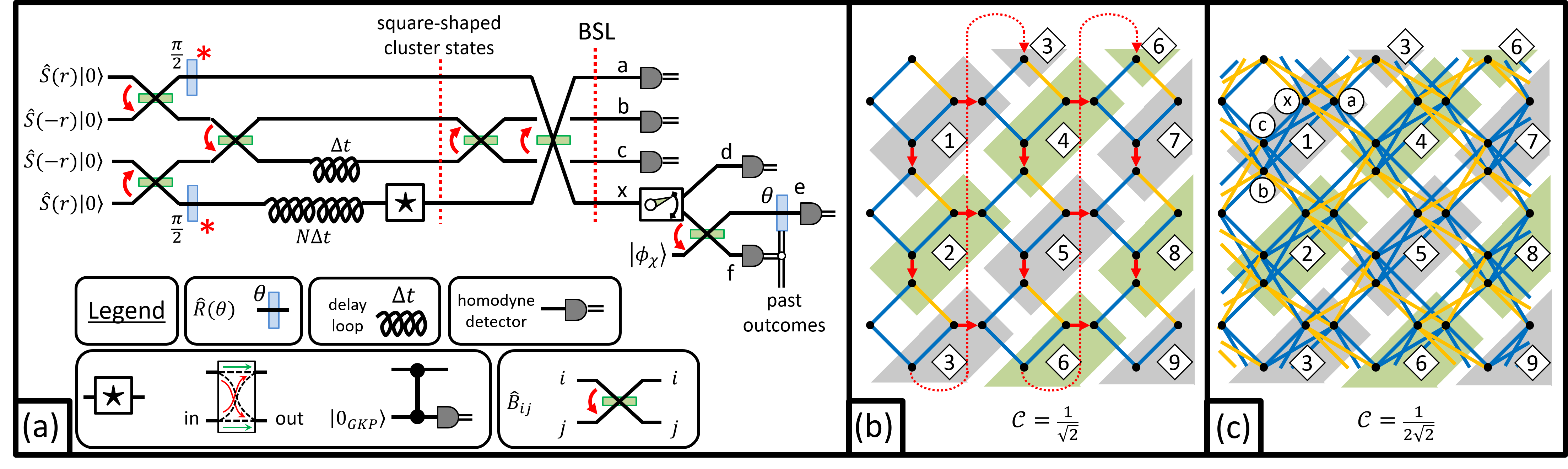
Figure 1: $\mathbf{(a)}$ Optical circuit diagram that executes all stages of the generation and measurement of the bilayer square lattice using temporal modes. Input states encoded within the cluster state can be addressed at the black star (“$\star$”). The legend includes two examples: (left) a switching device for encoding or removing inputs from the cluster state and (right) a syndrome-measurement circuit for quantum error correction using Gottesman-Kitaev-Preskill qubits Menicucci2014 . The first dashed red line indicates the point at which the state is made up of disjoint squares [see panel (b)]. The second dashed red line is the point where the final cluster state exists [see panel (c)]. Cluster-state modes are measured at detectors ‘a’, ‘b’, ‘c’, or ‘x’. Detector ‘x’ has two settings: homodyne measurement by using ‘d’ or cubic-phase gate-teleportation measurement by using ‘e’ and ‘f’. The latter involves injecting a cubic-phase-state ancilla $\ket{\phi_{\chi}}$ and using an adaptive (variable) phase delay. See main text for details. If the ‘x’ detector is always set to ‘d’, then the phase delays marked by a red asterisk can be omitted by compensating with a $\pi/4$ phase delay before detectors ‘a’, ‘b’, ‘c’, and ‘x’. $\mathbf{(b)}$ Each gray or green rectangle contains modes that arrive at the first red dotted line in panel (a) simultaneously. The numerical labels indicate the relevant time step in units of $\Delta t$. The red arrows between each disjoint square represent the application of the beamsplitters between the red dotted lines in panel (a). $\mathbf{(c)}$ The bilayer-square-lattice graph. The letters $\{\text{a},\text{b},\text{c},\text{x}\}$ in the rectangle labeled “1” indicate at which detector each mode is measured.

The first step in generating the BSL with temporal modes is to create a four-mode square-shaped cluster state. The construction of these is shown graphically as follows:

(15)

A pair of two-mode CVCSs [shown left] are transformed by a single 50:50 beamsplitter $\hat{B}_{ij}$ [indicated by the red (downward pointing) arrow from mode $i\rightarrow j$], resulting in the square-shaped cluster state [shown to the right in Eq. 15].

Using temporal modes with time-bin windows of size $\Delta t$, we can generate an array of square-shaped cluster states using the optical circuit shown in Fig. 1(a). Let $NM\Delta t$ be the runtime of the experiment, where $N$ sets the delay on the longer delay loop in Fig. 1(a). The time axis is partitioned into $M$ segments of length $N\Delta t$, yielding an array of size $N\times M$ in the time domain. In Fig. 1(b) we show the $N=M=3$ case as an example.

The final step involves applying a sequence of balanced beamsplitters between modes as indicated by the red arrows in Fig. 1(b). The resulting state has a double-layered square-lattice graph, as shown in Fig. 1(c). The experimental simplicity of our scheme is self-evident.

III.2 Nullifiers

Here we discuss the nullifiers of the BSL, which play an important role in verifying genuine multipartite entanglement via homodyne detection vanLoock2003 ; Walborn2009 ; Toscano2015 ; Gerke2016 . A class of experimentally convenient methods for verifying multiparite entanglement has been developed based on the van Loock-Furusawa criterion vanLoock2003 ; Yokoyama2013 . Such methods can be applied to states possessing a generating set of nullifiers $\{\hat{\nu}_{i}\}_{i=1,\dots n}$ with the property that each $\hat{\nu}_{i}$ is a linear combination of either position or momentum quadrature operators (not both). In this case, verifying multipartite entanglement requires only two types of homodyne measurements (on distinct copies of the state): all modes in the $\hat{q}$ basis or all modes in the $\hat{p}$ basis. Variances for all nullifiers can be inferred by taking linear combinations of the data, signaling the presence of multipartite entanglement vanLoock2003 .

The BSL graph $\mathbf{Z}_{\text{BSL}}$ in Fig. 1(c) immediately provides a set of $n$ generators for the algebra of nullifiers [see Eq. (14)]. These can be made Hermitian by taking the infinite-squeezing limit, $\mathbf{V}_{\text{BSL}}\coloneqq\lim_{r\rightarrow\infty}\mathbf{Z}_{\text{BSL}}$, resulting in approximate nullifiers Menicucci2011 :

$$\left(\hat{\mathbf{p}}-\mathbf{V}_{\text{BSL}}\hat{\mathbf{q}}\right)\ket{\psi_{\text{BSL}}}\to\mathbf{0}$$ (16)

where “$\to$” indicates the limit of infinite squeezing within $\ket{\psi_{\text{BSL}}}$ (which is independent of the limit used to define $\bm{\mathrm{V}}_{\text{BSL}}$). As noted above, it is more convenient from an experimental viewpoint to work with nullifiers that are combinations of either position or momentum operators. Though CVCSs cannot have such a set of nullifier generators Menicucci2011 , in some cases, we can use local phase delays (which preserve entanglement properties of the state) to transform them into states that do. This is formalized by the following theorem.

Theorem 1.

Any $2n$-mode, ideal (i.e., infinitely squeezed) continuous-variable (CV) cluster state with a trace-zero, self-inverse graph $\bm{\mathrm{V}}$ can be approximated by a $2n$-mode finitely-squeezed cluster state $\ket{\Psi_{r}}$, with overall squeezing parameter $r$, that is equivalent under local phase delays to a Gaussian pure state $\ket{\Phi_{r}}$ that satisfies the following two properties.

1. $\ket{\Phi_{r}}$ is approximately nullified by a set of $2n$ independent local operators that each consist of linear combinations of either position or momentum operators. Here locality is defined with respect to $\bm{\mathrm{V}}$.

2. The corresponding graph $\mathbf{Z}_{\Phi,r}$ only differs from $\mathbf{Z}_{\Psi,r}$ by a nonzero, uniform reweighting of the edges and a (different) nonzero, uniform reweighting of the self-loops.

For proof, see Appendix A.

The locality of these nullifiers tends to be a useful property when it comes to deriving bounds for entanglement witnesses based on the nullifier variances vanLoock2003 ; Yokoyama2013 . In the infinite-squeezing limit, the BSL graph is both self-inverse and trace zero. Therefore Theorem 1 applies.

Denote the BSL state by $\ket{\Psi_{\text{BSL}}}$. Following the abovementioned notational convention, we define the Gaussian pure state

$$\ket{\Phi_{\text{BSL}}}\coloneqq\hat{R}\left(\frac{\pi}{4}\right)^{\otimes 2n}\ket{\Psi_{\text{BSL}}}.$$ (17)

Though our proposal generates $\ket{\Psi_{\text{BSL}}}$, it could easily be modified [e.g., by including the local phase shifts in Eq. (17) at the BSL line in Fig. 1(a)] to generate $\ket{\Phi_{\text{BSL}}}$ instead. Furthermore, $\ket{\Phi_{\text{BSL}}}$ is an equivalent resource for measurement-based quantum computation and possesses a set of approximate nullifiers,

$$\begin{pmatrix}(\bm{\mathrm{I}}_{2n}-\bm{\mathrm{V}}_{\text{BSL}})\hat{\bm{\mathrm{p}}}\\ (\bm{\mathrm{I}}_{2n}+\bm{\mathrm{V}}_{\text{BSL}})\hat{\bm{\mathrm{q}}}\end{pmatrix}\ket{\Phi_{\text{BSL}}}\to\bm{\mathrm{0}},$$ (18)

that are experimentally convenient for entanglement verification.

Other known examples of cluster states with self-inverse, trace-zero graphs include the dual-rail wire Menicucci2011a ; Alexander2014 ; Wang2014 and the quad-rail lattice Menicucci2011a ; Alexander2016 ; Wang2014 .

IV Universal Measurement-based quantum computation

Now we describe universal quantum computation with the BSL. It was shown explicitly in Ref. Alexander2016b how arbitrary Gaussian unitary gates can be implemented on the BSL via homodyne detection. This analysis also included the effects of finite squeezing. Here we focus on extending this scheme by adding cubic-phase state injection for implementing non-Gaussian gates. With this resource, the only type of measurement our protocol requires is homodyne detection.

Temporal-mode architectures rely on fast control of the local-oscillator (LO) beam phase at each homodyne detector in order to set the measurement basis for each mode independently. Dynamic phase control for time bins of $~{}160$ ns (used in recent cluster-state demonstrations Yokoyama2013 ; Yoshikawa2016 ) is within the scope of current technology.

Just like conventional square-lattice cluster states Raussendorf2001 ; Menicucci2006 , the BSL can be treated as a collection of quantum wires embedded within a two-dimensional plane Alexander2016b . Entangling gates between these quantum wires are mediated by local projective measurements on sites that lie between wires. However, the BSL differs from other cluster states in that the quantum wires actually run along the diagonals of each square-like unit cell, rather than along the edges (which would be more conventional).

Each BSL lattice site, a.k.a. a macronode, consists of two modes, labeled $\alpha$ and $\beta$. Without loss of generality, assume that mode $\alpha$ is measured at either detector ‘x’ or detector ‘b’, and similarly, assume mode $\beta$ is measured at either ‘a’ or ‘c’. We define the symmetric (+) and anti-symmetric ($-$) mode of each macronode via:

$$\hat{a}_{\pm}\coloneqq\frac{1}{\sqrt{2}}(\hat{a}_{\alpha}\pm\hat{a}_{\beta})=\hat{B}_{\alpha\beta}\hat{a}_{\alpha(\beta)}\hat{B}_{\alpha\beta}^{\dagger}$$ (19)

This offers an alternative tensor-product decomposition of each macronode to the one provided by the physical modes, $\alpha$ and $\beta$. We divide the discussion of gate implementation into two parts: single-mode gates and two-mode gates. We leave an analysis of the finite-squeezing effects to future work.

IV.1 Single-mode gates

To implement single-mode gates, quantum wires must be decoupled from the rest of the lattice by deleting unwanted edges. This can be achieved by using detectors ‘b’ and ‘c’ to measure in the basis $\hat{q}[(-1)^{\xi}\frac{\pi}{4}]$ at particular macronodes, where $\xi$ is the time index modulo $N$ Alexander2016b . The decoupling of quantum wires is shown in Fig. 2(a). These wires are embedded versions of dual-rail wires Yokoyama2013 ; Alexander2014 , as shown in Fig. 2(b).

Input states can be injected into or removed from the BSL using the switching device at “$\star$” in Fig. 1(a). When embedded within the resource state, they reside in the “+” subspace of macronodes on the leftmost edge of the BSL. Phase-space displacements can be applied at the “$\star$” location, though this is equivalent to adapting the later measurements. We show this in Sec. IV.3.

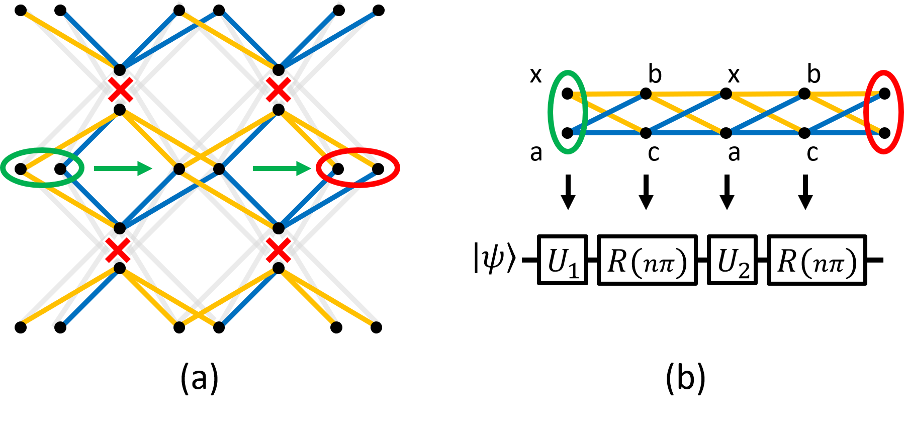
Figure 2: $\mathbf{(a)}$ Measuring $\hat{q}[(-1)^{\xi}\frac{\pi}{4}]$ at detectors ‘b’ and ‘c’ (indicated by a red ‘X’) at time index $\xi$ mod $N$ deletes the grayed-out edges Alexander2016b . This decouples the central three rows of nodes from the rest of the graph. An input state encoded within the green site on the left will propagate in the direction of the green arrows. $\mathbf{(b)}$ After deletion as in panel (a), the middle three graph modes are equivalent to the wire graph shown at the top. This state is known as the dual-rail wire Yokoyama2013 ; Alexander2014 . The letters {a, b, c, x} indicate the detector at which the relevant nodes are measured in Fig. 1(a). Measurements at detectors ‘x’ and ‘a’ can be chosen freely to implement gates, whereas measurement settings at ‘b’ and ‘c’ are fixed by the deletion measurements.

Measurement constraints.—Note that measurements at sites ‘b’ and ‘c’ are fixed because they are used to decouple the wires Alexander2016b . Therefore, only measurement degrees of freedom at ‘x’ and ‘a’ are available to implement single-mode gates.

Single-mode Gaussian unitaries.—Using the homodyne degrees of freedom both ‘a’ and ‘d’ (choosing the appropriate setting at ‘x’) implements a single-mode Gaussian unitary gate. Measuring $\hat{p}_{\text{d}}(\theta_{1})$ and $\hat{p}_{\text{a}}(\theta_{2})$ , with outcomes $m_{1}$ and $m_{2}$, respectively, at a site with an encoded input state implements the Gaussian unitary Alexander2016b

$$\hat{V}(\theta_{1},\theta_{2},m_{1},m_{2})$$ (20)

$$\coloneqq\hat{D}\left[\frac{-ie^{i\theta_{2}}m_{1}-ie^{i\theta_{1}}m_{2}}{\sin(\theta_{1}-\theta_{2})}\right]\hat{R}(\theta_{+})\hat{S}\left(\ln\tan{\theta_{-}}\right)\hat{R}(\theta_{+}),$$

where $\theta_{\pm}\coloneqq\frac{1}{2}(\theta_{1}\pm\theta_{2})$, and $\hat{D}(\alpha)\coloneqq\exp(\alpha\hat{a}^{\dagger}-\alpha^{*}\hat{a})$ is a displacement operator. Up to phase-space displacements, these gates can be used to generate arbitrary single-mode Gaussian unitaries Ukai2010 ; Alexander2014 .

Single-mode non-Gaussian unitaries.—Setting detector ‘x’ to measure at ‘e’ and ‘f’ can result in a non-Gaussian unitary operation. We set detectors ‘f’ and ‘a’ to measure in the $\hat{q}$ basis, and we set ‘e’ to measure $\hat{p}(\theta)$. Recall that we can treat the BSL as a collection of disjoint dual-rail wires (see Fig. 2).

In order to better analyze the effect of this measurement apparatus, in Fig. 3 we introduce some useful circuit identities. First, consider the following identities involving the $\hat{C}_{Z}$ gate (that follow from the gate definitions):

$$\hat{B}^{(\dagger)}_{jk}\hat{C}_{Z,ij}(g) =\hat{C}_{Z,ij}\left(\frac{g}{\sqrt{2}}\right)\hat{C}^{(\dagger)}_{Z,ik}\left(\frac{g}{\sqrt{2}}\right)\hat{B}^{(\dagger)}_{jk},$$ (21)

$${}_{q_{j}}\!\!\bra{s}\hat{C}_{Z,ij}(g) =\hat{Z}_{i}(sg)\,_{q_{j}}\!\!\bra{s},$$ (22)

shown in Fig. 3(a)–(c). Next, we define the operation

$$\mathcal{E}_{\ket{\varphi},m}\coloneqq\hat{X}(-m)\hat{S}\left(\ln\sqrt{2}\right)\varphi\left(m\sqrt{2}-\hat{q}\right),~{}$$ (23)

where $\varphi(s)={}_{q\!\!}\braket{s}{\varphi}$. In Appendix B we show that $\mathcal{E}_{\ket{\varphi},m}$ can be implemented using the circuit shown in Fig. 3(d), i.e.,

$$_{q_{k}}\!\!\bra{m}\hat{B}_{jk}\ket{\psi}_{j}\otimes\ket{\varphi}_{k} =\mathcal{E}_{\ket{\varphi},m}\ket{\psi}_{j}.$$ (24)

(Note that this is a trace-decreasing map, so for any particular outcome $m$, the state must be renormalized afterward.) Finally, Fig. 3(e) shows a measurement-based teleportation circuit Alexander2014 . In the infinite-squeezing limit, this implements

$$\hat{M}_{\theta,m}\coloneqq\hat{X}\left(-2m\sec\theta\right)\hat{R}\left(-\frac{\pi}{2}\right)\hat{S}\left(\ln\frac{1}{2}\right)\hat{P}(\tan\theta).$$ (25)

We provide a proof of Eq. (25) in Appendix C.

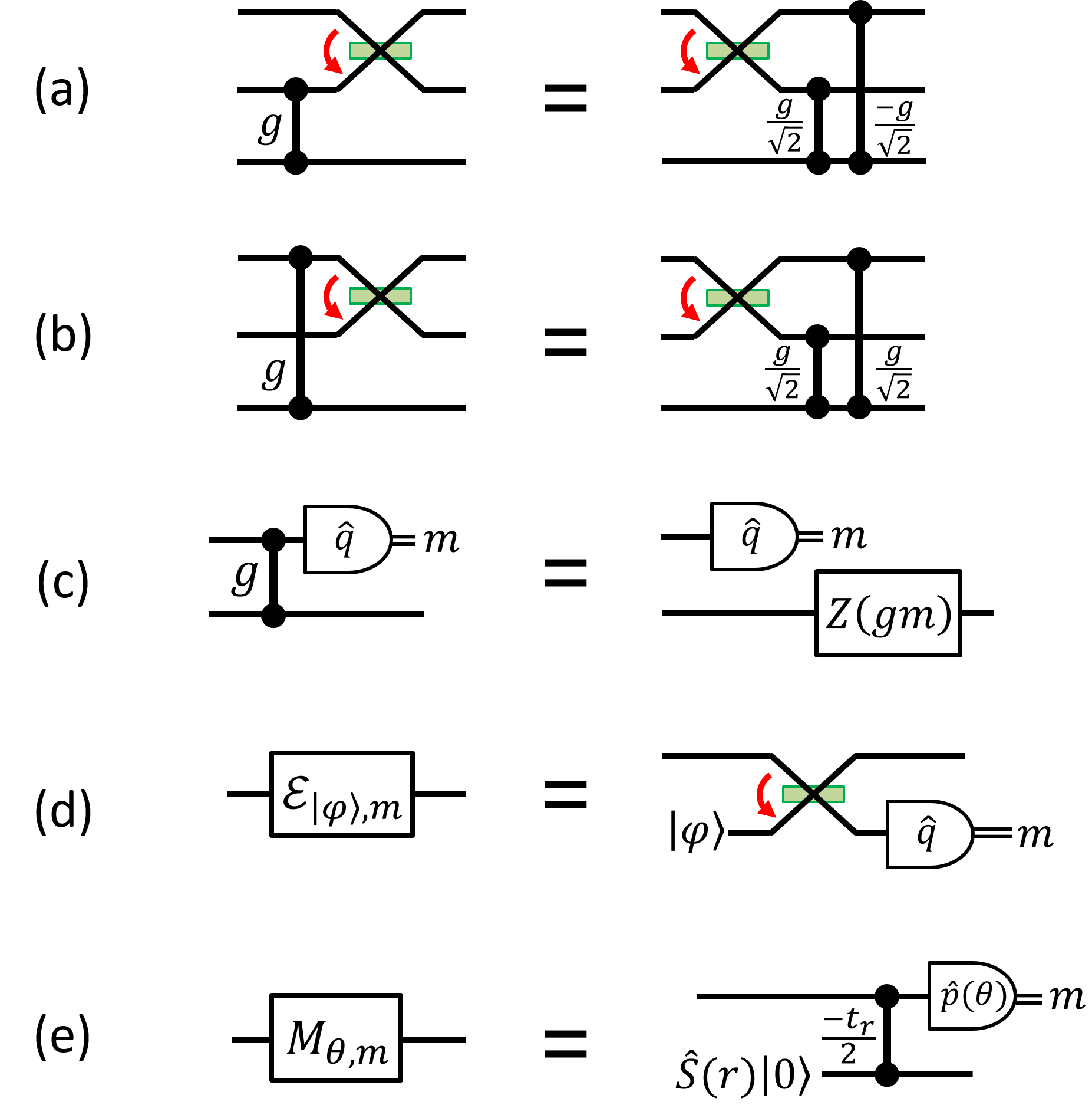
Figure 3: ($\mathbf{a}$) Commutation of the $\hat{C}_{Z}$ gate through $\hat{B}$ [Eq.(21)]. ($\mathbf{b}$) Commutation of the $\hat{C}_{Z}$ gate through $\hat{B}^{\dagger}$ [Eq.(21)]. ($\mathbf{c}$) $\hat{q}$-measurement after the $\hat{C}_{Z}$ gate [Eq.(22)]. ($\mathbf{d}$) Circuit implementation of the $\mathcal{E}$ operation [Eq. (24)]. ($\mathbf{e}$) Measurement-based teleportation identity [Eq. (25)].

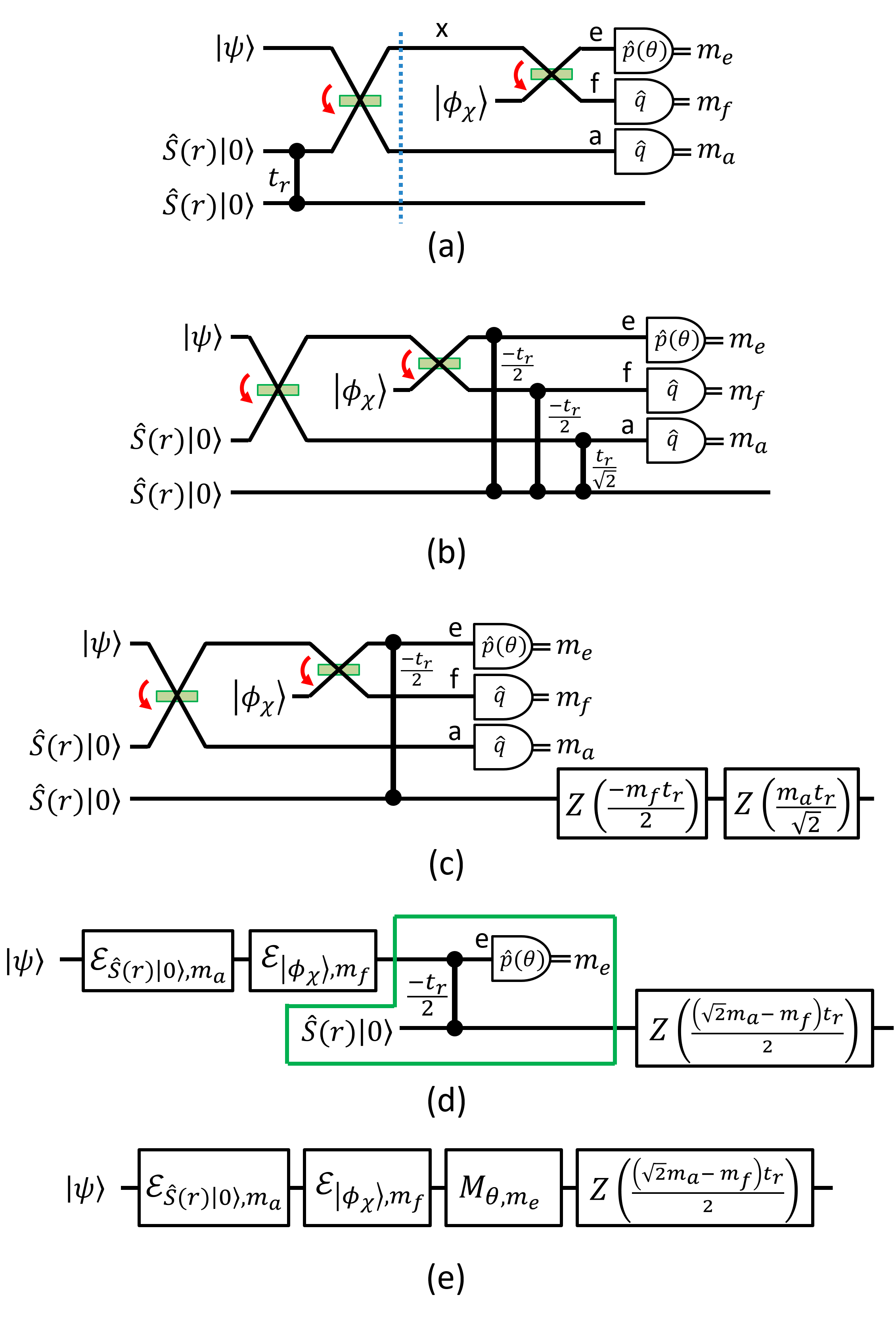
Figure 4: $\mathbf{(a)}$ This circuit is equivalent to performing non-Gaussian measurement on the BSL. For compactness, the conditional phase delay shown in Fig. 1(a) has been incorporated into the homodyne detector at ‘e’. The input $\ket{\psi}$ should be interpreted as occupying the symmetric subspace of modes ‘x’ and ‘a’ [Eq. 19]. Left of the dotted blue line, this circuit is equivalent to the macronode measurement circuit for a dual-rail wire Alexander2014 . The parameter $t_{r}=\tanh{2r}$ sets the strength of the $\hat{C}_{Z}(t_{r})$ gate. $\mathbf{(b)}$ Starting from panel (a), commute the $\hat{C}_{Z}$ gate rightwards past one beamsplitter [using Fig. 3(b)] and then past the other [using Fig. 3(c)]. The end result is three $\hat{C}_{Z}$ gates as shown. $\mathbf{(c)}$ Two of these $\hat{C}_{Z}$ gates precede a measurement in the $\hat{q}$ basis. We can use Fig. 3(d) to replace these with $\hat{Z}$ gates. $\mathbf{(d)}$ The green box is the measurement-based teleportation circuit [Eq. (25)]. $\mathbf{(e)}$ Final equivalent circuit, which implements $\hat{L}(\chi,\sigma,\bm{\mathrm{m}})$ [Eq. (IV.1)].

Now we analyze the measurement apparatus. Performing our non-Gaussian measurement procedure is equivalent to the quantum circuit shown in Fig. 4(a). This can be simplified by applying the above identities as described by Figs. 4(b)-(e). Fig. 4(e) shows that the measurement implements the following operation:

$$\hat{L}(\chi,\sigma,\mathbf{m}) \coloneqq$$

$$\hat{Z}\left(\frac{t_{r}\left(\sqrt{2}m_{a}-m_{f}\right)}{2}\right)\hat{M}_{(\tan^{-1}\sigma),m_{e}}\mathcal{E}_{\ket{\phi_{\chi}},m_{f}}\mathcal{E}_{\hat{S}(r)\ket{0},m_{a}}.$$ (26)

By performing some straightforward algebraic manipulations and taking the infinite squeezing limit, $\hat{L}$ can be simplified further to

$$\hat{L}(\chi,\sigma,\mathbf{m}) =$$

$$\hat{Z}\left(\sqrt{2}m_{a}\right)\hat{X}(\kappa)\hat{R}\left(-\frac{\pi}{2}\right)\hat{P}\left(\tau\right)\hat{K}\left(-2\sqrt{2}\chi\right),$$ (27)

where

$$\mathbf{m} \coloneqq(m_{a},m_{e},m_{f}),$$ (28)

$$\tau \coloneqq 4\sigma+4\chi\left(m_{a}+\sqrt{2}m_{f}\right),$$ (29)

$$\kappa \coloneqq-2m_{e}\sqrt{1+\sigma^{2}}-2\sigma\left({\sqrt{2}m_{a}+m_{f}}\right)$$

$$\qquad-\sqrt{2}\chi\left(m_{a}+\sqrt{2}m_{f}\right)^{2},$$ (30)

and we have neglected the overall phase. We have included a step-by-step proof in Appendix D for completeness.

The key feature of Eq. (27) is the cubic part, $\hat{K}(\chi)$, which extends our scheme beyond merely Gaussian quantum computation.

By sequentially applying the measurements described above to a wire [as in Fig. 2(b)], we can generate arbitrary single-mode unitary gates Lloyd1999 ; Gu2009 . Note that with bounded squeezing resources and without quantum error correction, the effective length of the possible quantum computation is bounded from above by a constant Ohliger2012 . However, by using encoded qubits Gottesman2001 , arbitrarily long qubit-level quantum computation is possible provided that the overall squeezing levels are sufficiently high and the effective qubit noise model is compatible with viable fault-tolerant quantum-error-correction strategies Menicucci2014 .

Next we show how to implement entangling operations using homodyne measurements.

IV.2 Entangling operations

On the BSL, it is possible to implement entangling operations using homodyne detectors Alexander2016b . Neighboring wires are naturally coupled by the BSL graph structure unless deletion measurements are applied, as described in the previous section.

By measuring a few columns of BSL modes, it is possible to implement Gaussian unitary gates that interact many modes at once. Because the form of such gates can be rather complicated (generally involving many modes and measurement angles), it is convenient to focus on the two-mode case, which is sufficient for demonstrating universality.

Consider the portion of the BSL shown in Fig. 5(a). Performing measurements of $[\hat{p}_{\alpha}(\theta_{2\alpha}),\hat{p}_{\beta}(\theta_{2\beta})]$, $[\hat{p}_{\alpha}(\theta_{3\alpha}),\hat{p}_{\beta}(\theta_{3\beta})]$, and $[\hat{p}_{\alpha}(\theta_{4\alpha}),\hat{p}_{\beta}(\theta_{4\beta})]$ on macronodes 2, 3, and 4, respectively, implements a sequence of beamsplitter and $\hat{V}$ gates [see Eq. (20)],

$$\hat{B}_{2+,4+}\hat{V}_{2+}\left[(-1)^{k}\frac{\pi}{4},\theta_{3\alpha},m_{1\beta},m_{3\alpha}\right]$$

$$\qquad\times\hat{V}_{4+}\left[\theta_{3\beta},(-1)^{k}\frac{\pi}{4},m_{3\beta},m_{5\alpha}\right]$$

$$\qquad\times\hat{B}_{2+,4+}\hat{V}_{2+}(\theta_{2\alpha},\theta_{2\beta},m_{2\alpha},m_{2\beta})$$

$$\qquad\times\hat{V}_{4+}(\theta_{4\alpha},\theta_{4\beta},m_{4\alpha},m_{4\beta})$$ (31)

on inputs initially encoded within the symmetric subspace of macronodes 2 and 4 (denoted by the subscripts 2+ and 4+, respectively) Alexander2016b . Above, $k$ denotes the time index of macronode 2. Next, we consider two examples of gates included in this class.

If $\theta_{3\alpha}=\theta_{3\beta}=(-1)^{k+1}\frac{\pi}{4}$ in Eq. (31) then up to displacements and overall phase,

$$\left(\hat{V}\otimes\hat{V}\right)\hat{B}=\hat{B}^{\dagger}\left(\hat{V}\otimes\hat{V}\right)$$ (32)

(we omit subscripts and dependence on measurement variables). Thus, Eq. (31) is reduced to two copies of the single-mode gate case described in the previous section.

By brute-force search we found that choosing

$$\begin{pmatrix}\theta_{2\alpha}\\ \theta_{2\beta}\\ \theta_{3\alpha}\\ \theta_{3\beta}\\ \theta_{4\alpha}\\ \theta_{4\beta}\end{pmatrix}=\begin{pmatrix}(-1)^{k+1}\frac{\pi}{8}\\ (-1)^{k}\frac{3\pi}{8}\\ (-1)^{k}\frac{\pi}{4}+\phi\\ (-1)^{k}\frac{\pi}{4}-\phi\\ (-1)^{k+1}\frac{\pi}{8}\\ (-1)^{k}\frac{3\pi}{8}\end{pmatrix}$$ (33)

simplifies the gate in Eq. (31) to a gate of the form

$$\left[\hat{X}(\lambda_{1})\hat{Z}(\lambda_{2})\otimes\hat{X}(\lambda_{3})\hat{Z}(\lambda_{4})\right]$$

$$\times\left[\hat{R}\left((-1)^{k+1}\frac{3\pi}{4}\right)\otimes\hat{R}\left((-1)^{k}\frac{\pi}{4}\right)\right]\hat{C}_{Z}(2\cot{\phi})$$ (34)

for some $\lambda_{1}$, $\lambda_{2}$, $\lambda_{3}$, and $\lambda_{4}$ Alexander2016b .

Note that this implements a $\hat{C}_{Z}$ gate (of variable weight) up to a pair of local phase delays. These phase delays can be undone using measurements further along the BSL, such as with gates $\hat{U}_{1}$ and $\hat{U}_{2}$ in Fig. 5(b).

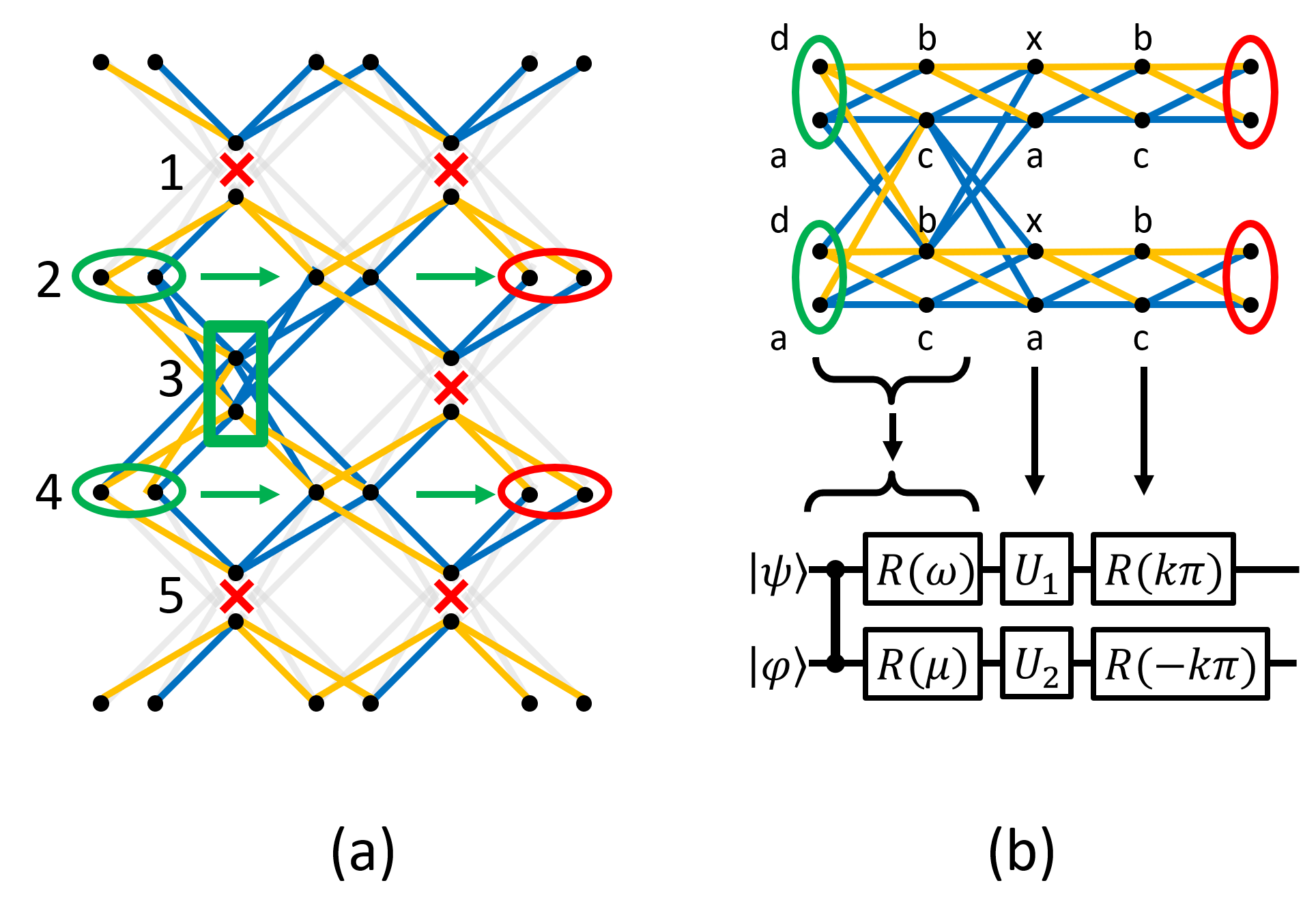
Figure 5: $\mathbf{(a)}$ Sublattice containing a region used to implement an entangling gate by measurement-based quantum computation. Detectors ‘b’ and ‘c’ measure $\hat{q}[(-1)^{n}\frac{\pi}{4}]$ at sites marked with a red ‘X’, thereby deleting the grayed-out links. Measurement of macronodes 2, 3, and 4, is described in the main text. The measurements on all other modes can be chosen freely. $\mathbf{(b)}$ After the deletion in panel (a), the middle six rows of modes are equivalent to this subgraph. Measurements on this resource state can implement circuits as shown. Here, the $\hat{C}_{Z}(g)$ gate has weight $g=2\cot{\phi}$. Also, $\omega=(-1)^{k+1}\tfrac{3\pi}{4}$ and $\mu=(-1)^{k}\tfrac{\pi}{4}$.

IV.3 Adaptivity of the measurement outcomes

Above we described how to implement a universal set of gates [see Eqs. (20), (27), and (34)]. In each case, however, the gate has only been implemented up to a known phase-space displacement that depends on the random measurement outcomes. To make computation deterministic, one can apply appropriate displacements at the “$\star$” site in Fig. 1(a) or use an adaptive measurement protocol—i.e., later measurement bases are chosen in a way that depends on the values of prior measurement outcomes Gu2009 .

Measurement protocols consisting only of homodyne measurements are an exception. They can be implemented deterministically without such adaptivity, though these protocols are not universal and only implement Gaussian unitary gates Menicucci2006 ; Gu2009 . To see this, note that the phase-space displacements form a normal subgroup of the Gaussian unitaries. Therefore, the randomness of the measurement outcomes only causes Gaussian computations to differ up to a final phase-space displacement. This in turn can then be dealt with by classically processing the final homodyne measurement data.

We now consider the case of implementing $\hat{L}(\chi,\sigma,\mathbf{m})$ from Eq. (27). Suppose that $\hat{X}(s)$ and $\hat{Z}(t)$ are unwanted phase-space displacements resulting from the previous step of MBQC. Now we consider commuting these so that they act after $\hat{L}(\chi,\sigma,\mathbf{m})$:

$$\hat{L}(\chi,\sigma,\mathbf{m})\hat{Z}(t)=\hat{X}(t)\hat{L}(\chi,\sigma,\mathbf{m}),$$ (35)

$$\hat{L}(\chi,\sigma,\mathbf{m})\hat{X}(s)$$

$$\quad=\hat{Z}(-s)\hat{X}(\tau s-2\sqrt{2}s^{2}\chi)\hat{L}\left(\chi,\sigma,\mathbf{m}\right)\hat{P}(-4\sqrt{2}s\chi),$$ (36)

where we neglect overall phases. Note that in the case of $\hat{Z}(t)$, commutation still results in a displacement operator. The $\hat{X}(s)$ case is more complicated, generating additional position and momentum displacements, as well as a shear. By adapting the homodyne measurement angle $\theta=\tan^{-1}\sigma$ in Eq. (36), we can cancel out the effect of the shear $\hat{P}(-4\sqrt{2}s\chi)$ at the price of an additional contribution to the final phase-space displacement. Modifying the shear parameter $\sigma\rightarrow\sigma^{\prime}=\sigma+\sqrt{2}s\chi$ in Eq. (36), equivalent to $\theta\to\theta^{\prime}=\tan^{-1}(\tan\theta+\sqrt{2}s\chi)$, and applying the appropriate commutation relations, we get

$$\hat{L}(\chi,\sigma^{\prime},\mathbf{m})\hat{X}(s) =\hat{Z}(-s)\hat{X}\left(\zeta\right)\hat{L}\left(\chi,\sigma,\mathbf{m}\right),$$ (37)

where

$$\zeta\coloneqq 4s\sigma+2\sqrt{2}s\chi(m_{f}+s)-2m_{e}(\sqrt{1+{\sigma^{\prime}}^{2}}-\sqrt{1+\sigma^{2}}).$$ (38)

In other words, by making detector ‘e’ (or equivalently, the parameter $\sigma$) adaptive, we can compensate control for random phase-space displacements and deterministically implement non-Gaussian unitary gates, up to a final known phase space displacement. This is the only type of adaptive measurement required by our protocol since unwanted displacements at the end of the computation can be dealt with by post-processing the measurement data Gu2009 .

Our approach is very similar to the adaptive homodyne techniques used in Ref. Miyata2016 for cubic-phase-gate teleportation. Implementing adaptive squeezing operations (e.g., at the location “$\star$”) is experimentally infeasible, so it is significant that our scheme only requires adaptive linear optics.

V Conclusion

Here we have proposed a method using temporal modes for generating the bilayer-square-lattice cluster state—a universal resource for measurement-based quantum computation Alexander2016b . Our scheme only requires four sources of squeezed vacuum modes (such as an optical parametric oscillator) and a few beamsplitters. The simplicity of this approach makes it a natural two-dimensional generalization of one-dimensional resource states generated in Refs. Yokoyama2013 ; Yoshikawa2016 .

We showed by using properties of the bilayer square lattice’s graph that it is equivalent under local phase delays to a Gaussian pure state that has essentially the same graph and possesses approximate local nullifiers composed purely of either position or momentum operators. The verification of genuine multipartite entanglement on cluster states that are equivalent to pairwise-squeezed states is experimentally straightforward: all modes are simply measured in the position and momentum basis and appropriate linear combinations are taken, whose variance is compared to an appropriate entanglement witness vanLoock2003 . Furthermore, these features are shared by an entire family of cluster states that approximate trace-zero, self-inverse, ideal (i.e., infinitely-squeezed) cluster states.

Our proposal extends previous work by explicitly incorporating non-Gaussian elements into the measurement devices Ukai2010 ; Ukai2011 ; Su2013 ; Miyata2014 ; Ferrini2013a ; Alexander2014 ; Yokoyama2015 ; Ferrini2016 ; Alexander2016 . Such elements enable universal quantum computation. Our approach conveniently minimizes the requirements of measurement adaptivity, potentially reducing the noise due to finite squeezing, although a proper analysis of this is left to future work. One additional advantage of the chosen gate set is that it is readily compatible with the universal gate set for the Gottesman-Kitaev-Preskill qubit Gottesman2001 , which is a key ingredient in the proof of fault-tolerant quantum computation using continuous-variable cluster states Menicucci2014 .

Appendix A Proof of Theorem 1

The theorem contains two claims. We prove them in order. Our proof of the first claim proceeds in three steps.

1. We directly construct a Gaussian pure state $\ket{\Psi_{r}}$ with graph $\bm{\mathrm{Z}}_{\Psi,r}$ from the ideal graph $\bm{\mathrm{V}}$ and prove that it meets the definition of an approximate CV cluster state whose ideal graph is $\bm{\mathrm{V}}$.

2. We construct $\ket{\Phi_{r}}$ by applying phase delays to $\ket{\Psi_{r}}$ and prove that we can define a set of approximate nullifiers for this state (that are exact in the infinite-squeezing limit) that contain position or momentum only (and no combinations of the two).

3. We construct new linear combinations of these nullifiers, without mixing position and momentum, and prove that this new set of nullifiers has its support limited to the neighborhood (as defined by $\bm{\mathrm{V}}$) of some particular node.

We define $\ket{\Psi_{r}}$ to be the Gaussian pure state whose graph is Menicucci2011

$$\bm{\mathrm{Z}}_{\Psi,r}\coloneqq i(\operatorname{sech}2r)\bm{\mathrm{I}}_{2n}+(\tanh 2r)\bm{\mathrm{V}}.$$ (39)

It follows that the set $\{\bm{\mathrm{Z}}_{\Psi,r}|r>0\}$ is a family of Gaussian pure states indexed by a real parameter $r$ (the overall squeezing parameter) such that

$$\lim_{r\to\infty}\bm{\mathrm{Z}}_{\Psi,r}=\bm{\mathrm{V}}.$$ (40)

Any member of this set meets the definition Menicucci2011 of an approximate CV cluster state with an ideal graph $\bm{\mathrm{V}}$. Therefore, $\ket{\Psi_{r}}$ is an approximate CV cluster state with an ideal graph $\bm{\mathrm{V}}$. This proves step (i).

Let

$$\hat{R}_{\theta}\coloneqq\hat{R}(\theta)$$ (41)

for brevity. We now define

$$\ket{\Phi_{r}} \coloneqq\hat{R}_{\pi/4}^{\otimes 2n}\ket{\Psi_{r}}.$$ (42)

Using the fact that

$$\bigl{(}\hat{R}_{\pi/4}^{\otimes 2n}\bigr{)}^{\dagger}\hat{\bm{\mathrm{x}}}\bigl{(}\hat{R}_{\pi/4}^{\otimes 2n}\bigr{)} =\frac{1}{\sqrt{2}}\begin{pmatrix}\bm{\mathrm{I}}_{2n}&-\bm{\mathrm{I}}_{2n}\\ \bm{\mathrm{I}}_{2n}&\bm{\mathrm{I}}_{2n}\end{pmatrix}\hat{\bm{\mathrm{x}}},$$ (43)

then the rule for updating the graph for a Gaussian pure state Menicucci2011 gives

$$\bm{\mathrm{Z}}_{\Phi,r} =(\bm{\mathrm{I}}_{2n}+\bm{\mathrm{Z}}_{\Psi,r})(\bm{\mathrm{I}}_{2n}-\bm{\mathrm{Z}}_{\Psi,r})^{-1}.$$ (44)

To simplify this, we note that, from the assumptions of the theorem, $\bm{\mathrm{V}}=\bm{\mathrm{V}}^{\mathrm{T}}=\bm{\mathrm{V}}^{-1}\in\mathbb{R}^{2n\times 2n}$ and $\exists\bm{\mathrm{L}}\in\mathrm{O}(2n)$ such that

$$\bm{\mathrm{V}}=\bm{\mathrm{L}}(\bm{\mathrm{I}}_{n}\oplus-\bm{\mathrm{I}}_{n})\bm{\mathrm{L}}^{\mathrm{T}},$$ (45)

where $\oplus$ represents the matrix direct sum (i.e., it creates a block-diagonal matrix). This particular form is guaranteed because $\operatorname{tr}\bm{\mathrm{V}}=0$ and all of $\bm{\mathrm{V}}$’s eigenvalues must be $\pm 1$. For brevity later, we also define

$$z_{\pm} \coloneqq i\operatorname{sech}2r\pm\tanh 2r,$$ (46)

for which we have the following identity:

$$\frac{1+z_{\pm}}{1-z_{\pm}}=ie^{\pm 2r}.$$ (47)

Using Eqs. (45) and (46), we can rewrite Eq. (39) as

$$\bm{\mathrm{Z}}_{\Psi,r} =\bm{\mathrm{L}}(z_{+}\bm{\mathrm{I}}_{n}\oplus z_{-}\bm{\mathrm{I}}_{n})\bm{\mathrm{L}}^{\mathrm{T}}.$$ (48)

Plugging Eq. (48) into Eq. (44) and using Eq. (47) gives

$$\bm{\mathrm{Z}}_{\Phi,r} =i\bm{\mathrm{L}}(e^{2r}\bm{\mathrm{I}}_{n}\oplus e^{-2r}\bm{\mathrm{I}}_{n})\bm{\mathrm{L}}^{\mathrm{T}}.$$ (49)

Since $\bm{\mathrm{Z}}_{\Phi,r}$ is purely imaginary, we already know Menicucci2011 that it contains only $q$-$q$ and $p$-$p$ correlations (i.e., no $q$-$p$ correlations). But we still need to calculate the nullifiers.

The exact nullifiers for $\bm{\mathrm{Z}}_{\Phi,r}$ can be obtained from the usual relation Menicucci2011

$$\bm{\mathrm{0}} =(\hat{\bm{\mathrm{p}}}-\bm{\mathrm{Z}}_{\Phi,r}\hat{\bm{\mathrm{q}}})\ket{\Phi_{r}},$$ (50)

which, after left multiplication by $$-\bm{\mathrm{Z}}_{\Phi,r}^{-1}$$, also implies

$$\bm{\mathrm{0}} =(-\bm{\mathrm{Z}}_{\Phi,r}^{-1}\hat{\bm{\mathrm{p}}}+\hat{\bm{\mathrm{q}}})\ket{\Phi_{r}}.$$ (51)

For brevity later on, let us denote the top and bottom halves of $\bm{\mathrm{L}}^{\mathrm{T}}$ by

$$\bm{\mathrm{L}}_{+}^{\mathrm{T}} \coloneqq\begin{pmatrix}\bm{\mathrm{I}}_{n}&\bm{\mathrm{0}}\end{pmatrix}\bm{\mathrm{L}}^{\mathrm{T}},$$ (52)

$$\bm{\mathrm{L}}_{-}^{\mathrm{T}} \coloneqq\begin{pmatrix}\bm{\mathrm{0}}&\bm{\mathrm{I}}_{n}\end{pmatrix}\bm{\mathrm{L}}^{\mathrm{T}}.$$ (53)

Multiplying Eqs. (50) and (51) on the left by $\bm{\mathrm{L}}_{-}^{\mathrm{T}}$ and $\bm{\mathrm{L}}_{+}^{\mathrm{T}}$, respectively, gives

$$\bm{\mathrm{0}} =\bm{\mathrm{L}}_{-}^{\text{T}}(\hat{\bm{\mathrm{p}}}-ie^{-2r}\hat{\bm{\mathrm{q}}})\ket{\Phi_{r}},$$ (54)

$$\bm{\mathrm{0}} =\bm{\mathrm{L}}_{+}^{\mathrm{T}}(ie^{-2r}\hat{\bm{\mathrm{p}}}+\hat{\bm{\mathrm{q}}})\ket{\Phi_{r}}.$$ (55)

In the limit $r\to\infty$, we get

$$\begin{pmatrix}\bm{\mathrm{L}}_{-}^{\mathrm{T}}\hat{\bm{\mathrm{p}}}\\ \bm{\mathrm{L}}_{+}^{\mathrm{T}}\hat{\bm{\mathrm{q}}}\end{pmatrix}\ket{\Phi_{r}}\to\bm{\mathrm{0}}.$$ (56)

This proves step (ii).

The final step is to find linear combinations of these nullifiers that (a) do not mix $\hat{q}$ and $\hat{p}$ and (b) are local with respect to $\bm{\mathrm{V}}$. The neighborhood of node $j$ with respect to $\bm{\mathrm{V}}$ is given by the nonzero entries of the $j$th row (or, equivalently, the $j$th column) of $\bm{\mathrm{V}}$.

Examining the structure of $\bm{\mathrm{V}}$ shown in Eq. (45), we see that

$$\bm{\mathrm{V}} =\bm{\mathrm{L}}_{+}\bm{\mathrm{L}}_{+}^{\mathrm{T}}-\bm{\mathrm{L}}_{-}\bm{\mathrm{L}}_{-}^{\mathrm{T}}.$$ (57)

Therefore, since $\bm{\mathrm{L}}_{\pm}^{\mathrm{T}}\bm{\mathrm{L}}_{\mp}=\bm{\mathrm{0}}$, we have $\bm{\mathrm{I}}_{2n}=\bm{\mathrm{V}}^{2}=\bm{\mathrm{L}}_{+}\bm{\mathrm{L}}_{+}^{\mathrm{T}}+\bm{\mathrm{L}}_{-}\bm{\mathrm{L}}_{-}^{\mathrm{T}}$, and thus,

$$\bm{\mathrm{L}}_{\pm}\bm{\mathrm{L}}_{\pm}^{\mathrm{T}} =\frac{1}{2}(\bm{\mathrm{I}}_{2n}\pm\bm{\mathrm{V}}).$$ (58)

Therefore, we can multiply Eq. (56) from the left by $2(\bm{\mathrm{L}}_{-}\oplus\bm{\mathrm{L}}_{+})$ to obtain

$$\begin{pmatrix}(\bm{\mathrm{I}}_{2n}-\bm{\mathrm{V}})\hat{\bm{\mathrm{p}}}\\ (\bm{\mathrm{I}}_{2n}+\bm{\mathrm{V}})\hat{\bm{\mathrm{q}}}\end{pmatrix}\ket{\Phi_{r}}\to\bm{\mathrm{0}}.$$ (59)

This proves step (iii) and therefore proves the first claim.

To prove the second claim, we simply evaluate Eq. (49):

$$\bm{\mathrm{Z}}_{\Phi,r} =i\bm{\mathrm{L}}(e^{2r}\bm{\mathrm{I}}_{n}\oplus e^{-2r}\bm{\mathrm{I}}_{n})\bm{\mathrm{L}}^{\mathrm{T}}$$

$$=i\exp(2r\bm{\mathrm{V}})$$

$$=i(\cosh 2r)\bm{\mathrm{I}}_{2n}+i(\sinh 2r)\bm{\mathrm{V}},$$ (60)

where we use the fact that $\bm{\mathrm{V}}^{2}=\bm{\mathrm{I}}_{2n}$ to obtain the last line. ∎

Appendix B Gate gadget action

Here we directly calculate the effect of the circuit shown in Fig. 3(d). The operation in Fig. 3(d) is given by

$$\mathcal{E}_{\ket{\varphi},m} \coloneqq\,_{q_{2}}\!\!\bra{m}\hat{B}_{1,2}\int\mathrm{d}s\,\varphi(s)\ket{s}_{q_{2}}.$$ (61)

$$=\int\mathrm{d}s\,\varphi(s)\,_{q_{2}}\!\!\bra{m}\hat{B}_{1,2}\int\mathrm{d}t\ket{t}_{p_{1}\,\,p_{1}}\!\!\braket{t}{s}_{q_{2}}$$ (62)

Using the fact that $\hat{B}_{1,2}\ket{t}_{p_{1}}\ket{s}_{q_{2}}$ is equivalent to an infinitely squeezed, displaced two-mode squeezed state (equivalent to an EPR state Einstein1935 ), i.e.,

$$\hat{B}_{1,2}\ket{t}_{p_{1}}\ket{s}_{q_{2}} =\hat{X}_{1}\left(\frac{-s}{\sqrt{2}}\right)\hat{X}_{2}\left(\frac{s}{\sqrt{2}}\right)\hat{Z}_{1}\left(\frac{t}{\sqrt{2}}\right)\hat{Z}_{2}\left(\frac{t}{\sqrt{2}}\right)\frac{1}{\sqrt{\pi}}\int^{\infty}_{-\infty}\mathrm{d}r\,\ket{r}_{q_{1}}\ket{r}_{q_{2}}$$ (63)

$$=\hat{X}_{1}\left(\frac{-s}{\sqrt{2}}\right)\hat{X}_{2}\left(\frac{s}{\sqrt{2}}\right)\frac{1}{\sqrt{\pi}}\int^{\infty}_{-\infty}\mathrm{d}r\,e^{i\sqrt{2}tr}\ket{r}_{q_{1}}\ket{r}_{q_{2}}$$ (64)

$$=\frac{1}{\sqrt{\pi}}\int^{\infty}_{-\infty}\mathrm{d}r\,e^{i\sqrt{2}tr}\left\lvert r-\frac{s}{\sqrt{2}}\right\rangle_{q_{1}}\left\lvert r+\frac{s}{\sqrt{2}}\right\rangle_{q_{2}},$$ (65)

we get that

$$\mathcal{E}_{\ket{\varphi},m} =\frac{1}{\sqrt{\pi}}\int\mathrm{d}s\,\varphi(s)\bra{m}_{q_{2}}\int\mathrm{d}t\int\mathrm{d}r\,e^{i\sqrt{2}tr}\left\lvert r-\frac{s}{\sqrt{2}}\right\rangle_{q_{1}}\left\lvert r+\frac{s}{\sqrt{2}}\right\rangle_{q_{2}}\,{}_{p_{1}}\!\!\bra{t}$$ (66)

$$=\frac{1}{\sqrt{\pi}}\int\mathrm{d}s\,\varphi(s)\int\mathrm{d}t\int\mathrm{d}r\,e^{i\sqrt{2}tr}\delta\left(m-r-\frac{s}{\sqrt{2}}\right)\left\lvert r-\frac{s}{\sqrt{2}}\right\rangle_{q_{1}}\,{}_{p_{1}}\!\!\bra{t}$$ (67)

$$=\frac{1}{\sqrt{\pi}}\int\mathrm{d}s\,\varphi(s)\int\mathrm{d}t\,e^{it(\sqrt{2}m-s)}\left\lvert m-\sqrt{2}s\right\rangle_{q_{1}}\,{}_{p_{1}}\!\!\bra{t}$$ (68)

Then, using that

$$\ket{s}_{q}=\frac{1}{\sqrt{2\pi}}\int\mathrm{d}t\,e^{-its}\ket{t}_{p},$$ (69)

this simplifies further:

$$\mathcal{E}_{\ket{\varphi},m} =\sqrt{2}\int\mathrm{d}s\left|m-\sqrt{2}s\right\rangle_{q_{1}\,\,q_{1}}\!\!\left\langle\sqrt{2}m-s\right\rvert\varphi(s)$$ (70)

$$=\sqrt{2}\hat{X}_{1}(-m)\int\mathrm{d}s\left|2m-\sqrt{2}s\right\rangle_{q_{1}\,\,q_{1}}\!\!\left\langle\sqrt{2}m-s\right\rvert\varphi\left(\sqrt{2}m-\hat{q}_{1}\right)$$ (71)

$$=\hat{X}_{1}(-m)\hat{S}_{1}\left(\ln\sqrt{2}\right)\int\mathrm{d}s\left|\sqrt{2}m-s\right\rangle_{q_{1}\,\,q_{1}}\!\!\left\langle\sqrt{2}m-s\right|\varphi\left(\sqrt{2}m-\hat{q}_{1}\right)$$ (72)

$$=\hat{X}_{1}(-m)\hat{S}_{1}\left(\ln\sqrt{2}\right)\varphi\left(\sqrt{2}m-\hat{q}_{1}\right),$$ (73)

in agreement with Eq. (23).

Appendix C Measurement-based circuit

Here we review the effective operation implemented by the circuit in Fig. 3(e) for an input state $\ket{\psi_{1}}$. After the $\hat{C}_{Z}$ gate, we consider measuring the top mode in the $\hat{P}^{\dagger}(\tan{\theta})\hat{p}\hat{P}(\tan{\theta})=\hat{p}+(\tan{\theta})\hat{q}$ basis, which is equivalent to measuring $\hat{p}(\theta)$, obtaining outcome $m$, which is multiplied by $\sec{\theta}$ to obtain the effective outcome $m^{\prime}=m\sec{\theta}$ of the desired measurement Menicucci2006 . The output state $\ket{\psi_{2}}$ is given by

$$\ket{\psi_{2}}_{k} \propto\,_{p_{j}}\!\!\bra{m^{\prime}}\hat{P}_{j}(\tan{\theta})\hat{C}_{Z}(g)\ket{\psi_{1}}_{j}\otimes\left(\exp\left[-\frac{\hat{q}_{k}^{2}}{2e^{2r}}\right]\ket{0}_{p_{k}}\right)$$ (74)

Taking the infinite squeezing limit ($r\rightarrow\infty$),

$$\lim_{r\rightarrow\infty}\ket{\psi_{2}}_{k} =\text{Pr}(m^{\prime})^{-\frac{1}{2}}\,_{p_{j}}\!\!\bra{m^{\prime}}\hat{C}_{Z}(g)\ket{\psi_{1}^{\prime}}_{j}\otimes\ket{0}_{p_{k}}.$$ (75)

where $\ket{\psi_{1}^{\prime}}\coloneqq\hat{P}(\tan{\theta})\ket{\psi_{1}}$ and where $\Pr(x)$ is the probability of outcome $x$ in the infinite squeezing limit. Next, we use squeezers and $\pi$-phase delays to convert the $\hat{C}_{Z}$ gate weight from $g\mapsto 1$

$$\lim_{r\rightarrow\infty}\ket{\psi_{2}}_{k} =\text{Pr}(m^{\prime})^{-\frac{1}{2}}\,_{p_{j}}\!\!\bra{m^{\prime}}\hat{S}_{k}^{\dagger}(\ln\left\lvert{g}\right\rvert)\hat{R}^{\dagger}_{k}(\operatorname{Im}\ln g)\hat{C}_{Z}(1)\hat{R}_{k}(\operatorname{Im}\ln g)\hat{S}_{k}(\ln\left\lvert{g}\right\rvert)\ket{\psi_{1}^{\prime}}_{j}\otimes\ket{0}_{p_{k}}$$ (76)

$$=\text{Pr}(m^{\prime})^{-\frac{1}{2}}\hat{S}_{k}\left(\ln\frac{1}{\left\lvert{g}\right\rvert}\right)\hat{R}^{\dagger}_{k}(\operatorname{Im}\ln g)\,_{p_{j}}\!\!\bra{m^{\prime}}\hat{C}_{Z}(1)\ket{\psi_{1}^{\prime}}_{j}\otimes\ket{0}_{p_{k}}.$$ (77)

The final part of this expression is the standard weight-1 canonical continuous-variable cluster state teleportation circuit Menicucci2006 ; Gu2009 . The output is well known:

$$\text{Pr}(m^{\prime})^{-\frac{1}{2}}\,_{p_{j}}\!\!\bra{m^{\prime}}\hat{C}_{Z}(1)\ket{\psi_{1}^{\prime}}_{j}\otimes\ket{0}_{p_{k}}=\hat{X}_{k}(m^{\prime})\hat{R}_{k}\left(\frac{\pi}{2}\right)\ket{\psi_{1}^{\prime}}_{k}.$$ (78)

Combining Eq. (78) with Eq. (77), plugging in $g=-t_{r}/2$, and taking the infinite squeezing limit results in

$$\lim_{r\rightarrow\infty}\ket{\psi_{2}} =\hat{S}(\ln 2)\hat{R}^{\dagger}(\pi)\hat{X}(m^{\prime})\hat{R}\left(\frac{\pi}{2}\right)\ket{\psi_{1}^{\prime}}$$ (79)

$$=\hat{S}(\ln 2)\hat{X}(-m^{\prime})\hat{R}\left(-\frac{\pi}{2}\right)\ket{\psi_{1}^{\prime}}$$ (80)

$$=\hat{X}(-2m^{\prime})\hat{R}\left(-\frac{\pi}{2}\right)\hat{S}\left(\ln\frac{1}{2}\right)\ket{\psi_{1}^{\prime}}$$ (81)

$$=\hat{X}\left(-2m\sec\theta\right)\hat{R}\left(-\frac{\pi}{2}\right)\hat{S}\left(\ln\frac{1}{2}\right)\hat{P}(\tan\theta)\ket{\psi_{1}}$$ (82)

$$=\hat{M}_{\theta,m}\ket{\psi_{1}}$$ (83)

in agreement with Eq. (25).

Appendix D Step-by-step simplification of $\hat{L}$

Here we begin with the sequence of operations implemented by Fig. 4(e) and show how it can be simplified to Eq. (27). For brevity in what follows, we define the following combinations of measurement outcomes:

$$m_{\pm}\coloneqq\frac{\sqrt{2}m_{a}\pm m_{f}}{2}.$$ (84)

Using this compact notation, we rewrite Eq. (IV.1) as

$$\hat{L}(\chi,\sigma,\mathbf{m}) =\hat{Z}(t_{r}m_{-}){\hat{M}_{(\tan^{-1}\sigma),m_{e}}}\mathcal{E}_{\ket{\phi_{\chi}},m_{f}}\mathcal{E}_{\hat{S}(r)\ket{0},m_{a}}.$$ (85)

For convenience, we repeat the definitions

$$\hat{M}_{\theta,m} \coloneqq\hat{X}(-2m\sec\theta)\hat{R}\left(-\frac{\pi}{2}\right)\hat{S}\left(\ln\frac{1}{2}\right)\hat{P}(\tan\theta),$$ (86)

$$\mathcal{E}_{\ket{\varphi},m} \coloneqq\hat{X}(-m)\hat{S}\left(\ln\sqrt{2}\right)\varphi\left(\sqrt{2}m-\hat{q}\right),$$ (87)

from Eqs. (25) and (23), respectively. For $\ket{\varphi}=\hat{S}(r)\ket{0}$, the $\varphi$ term in Eq. (87) is a normalized Gaussian envelope with variance $e^{2r}/2$. In the infinite squeezing limit, this term acts trivially and can be ignored.

Applying the relevant definitions and taking the infinite-squeezing limit gives

$$\hat{L}(\chi,\sigma,\mathbf{m}) \propto\hat{Z}(m_{-})\hat{X}\left(-2m_{e}\sqrt{1+\sigma^{2}}\right)\hat{R}\left(-\frac{\pi}{2}\right)\hat{S}\left(\ln\frac{1}{2}\right)\hat{P}(\sigma)\hat{X}(-m_{f})\hat{S}(\ln\sqrt{2})\phi_{\chi}\left(\sqrt{2}m_{f}-\hat{q}\right)\hat{X}(-m_{a})\hat{S}(\ln\sqrt{2}),$$ (88)

where the $\propto$ sign indicates that we have omitted the overall phase. Now, we commute the $\hat{S}(\ln\sqrt{2})$ gates leftwards so they cancel with $\hat{S}\left(\ln\frac{1}{2}\right)$, giving

$$\hat{L}(\chi,\sigma,\mathbf{m}) \propto\hat{Z}(m_{-})\hat{X}\left(-2m_{e}\sqrt{1+\sigma^{2}}\right)\hat{R}\left(-\frac{\pi}{2}\right)\hat{P}(4\sigma)\hat{X}\left(\frac{-m_{f}}{2}\right)\phi_{\chi}\left(\sqrt{2}\left(m_{f}-\hat{q}\right)\right)\hat{X}\left(\frac{-m_{a}}{\sqrt{2}}\right).$$ (89)

Next, we commute displacements to the left, step by step:

$$\hat{L}(\chi,\sigma,\mathbf{m}) \propto\hat{Z}\left(m_{-}\right)\hat{X}\left(-2m_{e}\sqrt{1+\sigma^{2}}\right)\hat{R}\left(-\frac{\pi}{2}\right)\hat{P}(4\sigma)\hat{X}\left(-m_{+}\right)\phi_{\chi}\left(\sqrt{2}\left(m_{f}-\hat{q}\right)+m_{a}\right)$$ (90)

$$\propto\hat{Z}\left(m_{-}\right)\hat{X}\left(-2m_{e}\sqrt{1+\sigma^{2}}\right)\hat{R}\left(-\frac{\pi}{2}\right)\hat{X}\left(-m_{+}\right)\hat{Z}\left(-4\sigma m_{+}\right)\hat{P}(4\sigma)\phi_{\chi}\left(\sqrt{2}\left(m_{f}-\hat{q}\right)+m_{a}\right)$$ (91)

$$\propto\hat{Z}\left(\sqrt{2}m_{a}\right)\hat{X}\left[-2m_{e}\sqrt{1+\sigma^{2}}-2\sigma\left(\sqrt{2}m_{a}+m_{f}\right)\right]\hat{R}\left(-\frac{\pi}{2}\right)\hat{P}(4\sigma)\phi_{\chi}\left(\sqrt{2}\left(m_{f}-\hat{q}\right)+m_{a}\right)$$ (92)

Using $\phi_{\chi}(s)=e^{i\chi s^{3}/3}$, the rightmost term in Eq. (92) can be expanded as

$$\phi_{\chi}\left(\sqrt{2}\left(m_{f}-\hat{q}\right)+m_{a}\right) =e^{i\frac{\chi}{3}\left(\sqrt{2}\left(m_{f}-\hat{q}\right)+m_{a}\right)^{3}}$$ (93)

$$=\text{(phase)}\,e^{-i\sqrt{2}\chi(m_{a}+\sqrt{2}m_{f})^{2}\hat{q}}e^{i(2\chi m_{a}+2\sqrt{2}\chi m_{f})\hat{q}^{2}}e^{-i\frac{2\sqrt{2}\chi}{3}\hat{q}^{3}}$$ (94)

$$=\text{(phase)}\,\hat{Z}\left[-\sqrt{2}\chi\left(m_{a}+\sqrt{2}m_{f}\right)^{2}\right]\hat{P}\left(4\chi m_{a}+4\sqrt{2}\chi m_{f}\right)\hat{K}\left(-2\sqrt{2}\chi\right).$$ (95)

Once plugged into Eq. (92), the $\hat{Z}$ operator can be commuted to the left. We now give the final result:

$$\hat{L}(\chi,\sigma,\mathbf{m}) =\hat{Z}\left(\sqrt{2}m_{a}\right)\hat{X}(\kappa)\hat{R}\left(-\frac{\pi}{2}\right)\hat{P}\left[4\sigma+4\chi\left(m_{a}+\sqrt{2}m_{f}\right)\right]\hat{K}\left(-2\sqrt{2}\chi\right),$$ (96)

where we have now neglected (rather than merely omitted) the overall phase, and where

$$\kappa=-2m_{e}\sqrt{1+\sigma^{2}}-2\sigma(\sqrt{2}m_{a}+m_{f})-\sqrt{2}\chi(m_{a}+\sqrt{2}m_{f})^{2}$$ (97)

from Eq. (IV.1). This result is reported in Eq. (27).

References

• (1) N. C. Menicucci et al., “Universal quantum computation with continuous-variable cluster states”, Phys. Rev. Lett. 97, 110501 (2006).
• (2) R. Raussendorf and H. J. Briegel, “A one-way quantum computer”, Phys. Rev. Lett. 86, 5188 (2001).
• (3) M. L. Gu, C. Weedbrook, N. C. Menicucci, T. C. Ralph, and P. van Loock, “Quantum Computing with Continuous-Variable Clusters”, Phys. Rev. A 79, 062318 (2009).
• (4) M. Chen, N. C. Menicucci, and O. Pfister, “Experimental realization of multipartite entanglement of 60 modes of the quantum optical frequency comb”, Phys. Rev. Lett. 112, 120505 (2014).
• (5) S. Yokoyama et al., “Ultra-large-scale continuous-variable cluster states multiplexed in the time domain”, Nature Photon. 7, 982 (2013).
• (6) J. Yoshikawa et al., “Generation of one-million-mode continuous-variable cluster state by unlimited time-domain multiplexing”, APL Photonics 1, 060801 (2016).
• (7) N. C. Menicucci, S. T. Flammia, and P. van Loock, “Graphical calculus for Gaussian pure states”, Phys. Rev. A 83, 042335 (2011).
• (8) N. C. Menicucci, “Temporal-mode continuous-variable cluster states using linear optics”, Phys. Rev. A 83, 062314 (2011).
• (9) N. C. Menicucci, S. T. Flammia, and O. Pfister, “One-Way Quantum Computing in the Optical Frequency Comb”, Phys. Rev. Lett. 101, 130501 (2008).
• (10) S. T. Flammia, N. C. Menicucci, and O. Pfister, “The optical frequency comb as a one-way quantum computer”, J. Phys. B 42, 114009 (2009).
• (11) N. C. Menicucci, S. T. Flammia, H. Zaidi, and O. Pfister, “Ultracompact generation of continuous-variable cluster states”, Phys. Rev. A 76, 010302(R) (2007).
• (12) A. L. Grimsmo and A. Blais, “Squeezing and quantum state engineering with Josephson traveling wave amplifiers”, npj Quantum Inf. 3, 20 (2017).
• (13) P. Wang, M. Chen, N. C. Menicucci, and O. Pfister, “Weaving quantum optical frequency combs into continuous-variable hypercubic cluster states”, Phys. Rev. A 90, 032325 (2014).
• (14) R. N. Alexander et al., “One-way quantum computing with arbitrarily large time-frequency continuous-variable cluster states from a single optical parametric oscillator”, Phys. Rev. A 94, 032327 (2016).
• (15) S. Lloyd and S. L. Braunstein, “Quantum computation over continuous variables”, Phys. Rev. Lett. 82, 1784 (1999).
• (16) R. Filip, P. Marek, and U. L. Andersen, “Measurement-induced continuous-variable quantum interactions”, Phys. Rev. A 71, 042308 (2005).
• (17) J. Yoshikawa et al., “Demonstration of deterministic and high fidelity squeezing of quantum information”, Phys. Rev. A 76, 60301 (2007).
• (18) J. I. Yoshikawa, Y. Miwa, R. Filip, and A. Furusawa, “Demonstration of a reversible phase-insensitive optical amplifier”, Phys. Rev. A 83, 052307 (2011).
• (19) M. Yukawa et al., “Generating superposition of up-to three photons for continuous variable quantum information processing”, Opt. Express 21, 5529 (2013).
• (20) M. Yukawa et al., “Emulating quantum cubic nonlinearity”, Phys. Rev. A 88, 053816 (2013).
• (21) K. Marshall, R. Pooser, G. Siopsis, and C. Weedbrook, “Repeat-until-success cubic phase gate for universal continuous-variable quantum computation”, Phys. Rev. A 91, 032321 (2015).
• (22) K. Miyata et al., “Implementation of a quantum cubic gate by an adaptive non-Gaussian measurement”, Phys. Rev. A 93, 022301 (2016).
• (23) F. Arzani, N. Treps, and G. Ferrini, “Polynomial approximation of non-Gaussian unitaries by counting one photon at a time”, arXiv:1703.06693 (2017).
• (24) J. Yoshikawa et al., “Demonstration of a Quantum Nondemolition Sum Gate”, Phys. Rev. Lett. 101, 250501 (2008).
• (25) R. Ukai, J. Yoshikawa, N. Iwata, P. van Loock, and A. Furusawa, “Universal linear Bogoliubov transformations through one-way quantum computation”, Phys. Rev. A 81, 032315 (2010).
• (26) R. Ukai et al., “Demonstration of unconditional one-way quantum computations for continuous variables”, Phys. Rev. Lett. 106, 240504 (2010).
• (27) X. Su et al., “Gate sequence for continuous variable one-way quantum computation”, Nat. Commun. 4, 2828 (2013).
• (28) K. Miyata et al., “Experimental realization of a dynamic squeezing gate”, Phys. Rev. A 90, 060302 (2014).
• (29) G. Ferrini, J. P. Gazeau, T. Coudreau, C. Fabre, and N. Treps, “Compact Gaussian quantum computation by multi-pixel homodyne detection”, New J. Phys. 15, 093015 (2013).
• (30) R. N. Alexander, S. C. Armstrong, R. Ukai, and N. C. Menicucci, “Noise analysis of single-mode Gaussian operations using continuous-variable cluster states”, Phys. Rev. A 90, 062324 (2014).
• (31) S. Yokoyama et al., “Demonstration of a fully tunable entangling gate for continuous-variable one-way quantum computation”, Phys. Rev. A 92, 032304 (2015).
• (32) G. Ferrini, J. Roslund, F. Arzani, C. Fabre, and N. Treps, “Direct approach to Gaussian measurement based quantum computation”, Phys. Rev. A 94, 062332 (2016).
• (33) R. N. Alexander and N. C. Menicucci, “Flexible quantum circuits using scalable continuous-variable cluster states”, Phys. Rev. A 93, 062326 (2016).
• (34) S. D. Bartlett and B. C. Sanders, “Efficient classical simulation of optical quantum information circuits”, Phys. Rev. Lett. 89, 207903 (2002).
• (35) J. Yoshikawa et al., “Creation, Storage, and On-Demand Release of Optical Quantum States with a Negative Wigner Function”, Phys. Rev. X 3, 041028 (2013).
• (36) D. Gottesman, A. Kitaev, and J. Preskill, “Encoding a qubit in an oscillator”, Phys. Rev. A 64, 012310 (2001).
• (37) N. C. Menicucci, “Fault-Tolerant Measurement-Based Quantum Computing with Continuous-Variable Cluster States”, Phys. Rev. Lett. 112, 120504 (2014).
• (38) P. van Loock and A. Furusawa, “Detecting genuine multipartite continuous-variable entanglement”, Phys. Rev. A 67, 052315 (2003).
• (39) S. P. Walborn, B. G. Taketani, A. Salles, F. Toscano, and R. L. De Matos Filho, “Entropic Entanglement Criteria for Continuous Variables”, Phys. Rev. Lett. 103, 160505 (2009).
• (40) F. Toscano, A. Saboia, A. T. Avelar, and S. P. Walborn, “Systematic construction of genuine-multipartite-entanglement criteria in continuous-variable systems using uncertainty relations”, Phys. Rev. A 92, 052316 (2015).
• (41) S. Gerke et al., “Multipartite Entanglement of a Two-Separable State”, Phys. Rev. Lett. 117, 110502 (2016).
• (42) Y. Shiozawa et al., “Quantum Nondemolition Gate Operations and Measurements in Real Time on Fluctuating Signals”, (2017), arXiv:1712.08411.
• (43) M. Ohliger and J. Eisert, “Efficient measurement-based quantum computing with continuous-variable systems”, Physical Review A 85, 062318 (2012).
• (44) A. Einstein, B. Podolsky, and N. Rosen, “Can Quantum-Mechanical Description of Physical Reality Be Considered Complete?”, Phys. Rev. 47, 777 (1935).