Revival of the Deser-Woodard nonlocal gravity model:
Comparison of the original nonlocal form and a localized formulation
Abstract
We examine the origin of two opposite results for the growth of perturbations in the Deser-Woodard (DW) nonlocal gravity model. One group previously analyzed the model in its original nonlocal form and showed that the growth of structure in the DW model is enhanced compared to general relativity (GR) and thus concluded that the model was ruled out. Recently, however, another group has reanalyzed it by localizing the model and found that the growth in their localized version is suppressed even compared to the one in GR. The question was whether the discrepancy originates from an intrinsic difference between the nonlocal and localized formulations or is due to their different implementations of the sub-horizon limit. We show that the nonlocal and local formulations give the same solutions for the linear perturbations as long as the initial conditions are set the same. The different implementations of the sub-horizon limit lead to different transient behaviors of some perturbation variables; however, they do not affect the growth of matter perturbations at the sub-horizon scale much. In the meantime, we also report an error in the numerical calculation code of the former group and verify that after fixing the error the nonlocal version also gives the suppressed growth. Finally, we discuss two alternative definitions of the effective gravitational constant taken by the two groups and some open problems.
I Introduction
Nonlocal modifications of gravity as an account for the current phase of cosmic acceleration have recently received significant attention DW-2007 ; Joukovskaya-2007 ; NO-2007 ; CMN-2008 ; NO-2008 ; Koivisto-0803 ; ghost-nonlocal-Koivisto-0807 ; CENO-2009 ; Koshelev-2009 ; DW-2009 ; Biswas-2010 ; ghost-nonlocal-NOSZ-1010 ; Bamba-1104 ; Barvinsky-1107 ; ghost-nonlocal-ZS-1108 ; EPV-1110 ; Barvinsky-1112 ; PD-2012 ; Barvinsky-1209 ; EPV-1209 ; EPVZ-1302 ; Maggiore-1307 ; DW-2013 ; DP-2013 ; Maggiore-1311.3421 ; Maggiore-1311.3435 ; W-review-2014 ; Maggiore-1401 ; MM-2014 ; Maggiore-1403 ; Koivisto-1406 ; BLHBP-1408 ; DM-1408 ; Maggiore-1411 ; ZWLLCCS-1511 ; Maggiore-1512 ; ZKSZ-1601 ; Maggiore-1602.01078 ; Maggiore-1602.03558 ; Maggiore-1603 ; NAAKR-1606 ; Maggiore-review ; PS-2016 ; WZWZC-1611 ; NCA-2017 ; DDSKR-1701 ; VAAS-2017 ; Dirian-1704 ; ABN-1707 ; Roobiat-2017 ; ZWYZCZ-2017 ; Sebastian-1708 ; Sebastian-1709 ; Bamba-1711 . 111For nonlocal gravity with more quantum field theory oriented approaches, see Refs. Parker-1985 ; Banks-1988 ; Wetterich-1998 ; Barvinsky-2003 ; Hamber-2005 ; Biswas-2006 ; Mazzitelli-2007 ; Ferreira-2013 ; Donoghue-2014 ; Calmet-2015 ; Donoghue-2015 ; Oda-1704 ; Oda-1706 ; Oda-1709 ; Mazzitelli-2017 ; Bautista-2017 ; Calmet-2017 ; Oda-1711 ; as an account for inflation, see Refs. NO-2007 ; TW-0904 ; TW-1006 ; TW-1405 ; KKM-1604 ; TW-1606 ; and for dark matter, see Refs. SW-2003 ; DEW-1106 ; W-MOND-review-1403 ; DEW-1405 ; KRSTWX-1608 . One such attempt is a model proposed by Deser and Woodard, in which a nonlocal piece in the form of is added to the Einstein-Hilbert term DW-2007 . Here, is a free function with the nonlocal argument, the inverse scalar d’Alembertian acting on the Ricci scalar.
An advantage of leaving as an arbitrary function is that can be constructed to reproduce any desirable expansion history. A generic technique for how to tune the function for any given expansion history has been provided in Ref. DW-2009 . 222Similar reconstruction techniques are found in Refs. EPV-1209 ; EPVZ-1302 . Applying this technique to the special case of Lambda-cold-dark-matter (CDM) cosmology, the authors of DW-2009 have obtained a numerical solution for that exactly reproduces the expansion history of CDM without a cosmological constant. This implies that one does not test the Deser-Woodard (DW) model with background expansion data. One rather fixes the model by adjusting the function such that its background is identical to the given expansion and then examines how perturbations grow. A key aspect is that, even though its background expansion is the same as in GR, the growth of perturbations in the DW model is different from the growth in general relativity (GR). Whether one fixes its background to the CDM expansion history as in Refs. PD-2012 ; DP-2013 ; NCA-2017 or to some non-CDM as in Ref. PS-2016 , one gets different structure formation from that in GR. Thus, the model is testable with growth data (but not with expansion data).
This is a distinct feature of the DW nonlocal model. Other classes of nonlocal models, for instance, the model proposed by Maggiore and Mancarella MM-2014 or model by Vardanyan et al. VAAS-2017 , do not reproduce a chosen background expansion. Thus, one tests these nonlocal models with both expansion and growth data. However, in practice, one first fixes the value (or range) of the parameter in such a way that the model describes the expansion data as closely as possible and then investigates how perturbations evolve. Therefore, when it comes to testing the growth of perturbations, no free parameter (or free function in the case of the DW model) is left. The models then make their unique predictions for the growth, which distinguish them from each other.
In this regard, measuring the growth of structure is a powerful test that can decisively rule out a gravity model Bertschinger-2006 ; Hu-Sawicki-0708 ; Baker:2012zs ; Huterer:2013xky . For the DW nonlocal gravity model, two groups (one in its original nonlocal form PD-2012 ; DP-2013 and the other in a localized version NCA-2017 ) have studied its prediction for the growth once the background expansion was fixed to the one of CDM, and they have obtained results opposite of one another. The reason for this discrepancy has been suspected whether it is due to an intrinsic difference between the nonlocal and localized formulations, or it is due to their different implementations of the sub-horizon limit. In the present paper, we thoroughly examine the two formulations and the different approximations that they have taken for the sub-horizon scale.
II Model and Zeroth-Order Equations
The DW model nonlocally modifies the Einstein-Hibert action as DW-2007
| (1) |
where is a function of the inverse d’Alembertian acting on the Ricci scalar that will be determined by matching a given expansion history. Note that the argument is dimensionless, thus no new mass scale is introduced in the action. By varying the action with respect to the metric and imposing the retarded boundary conditions, 333The retarded boundary condition on Green’s function ensures the field equations are causal. Note also that Green’s function being the inverse of a differential operator, is sufficient for conservation. Hence, the resulting field equations are causal and conserved. See Ref. W-review-2014 for more discussions on the causality and conservation. one obtains the modified Einstein equations
| (2) |
where the correction to the Einstein tensor is DW-2007
| (3) |
Here, a prime means a derivative of the function with respect to the argument. Applying the field equations (2) to the Friedman-Lemaître-Robertson-Walker (FLRW) metric,
| (4) |
leads to
| (5) | |||||
| (6) |
Here, and are the energy density and pressure of a perfect fluid and we denote quantities in the FLRW background with overbars to distinguish them from perturbed quantities. The zeroth-order corrections are DW-2007
| (7) | |||||
| (8) |
II.1 Localization
One can localize the nonlocal field equations by introducing two auxiliary variables and defined as, following the notation of Ref. NCA-2017 ,
| (9) | |||||
| (10) |
Also, we denote the operator acting on the nonlocal function as
| (11) |
In this notation, the modified Einstein tensor is simply written as
| (12) |
and the zeroth-order corrections (7) and (8) become
| (13) | |||||
| (14) |
We then have the zeroth-order modified Einstein equations
| (15) | |||||
| (16) |
accompanied by the zeroth-order auxiliary field equations
| (17) | |||||
| (18) |
in this localized formulation.
II.2 Reconstruction of
The last step to finalize the zeroth-order equations is to reconstruct the free function for a given expansion history, for which Ref. DW-2009 provides a general technique. That is, one can solve a differential equation for as the following integral (see Eq. (43) of Ref. DW-2009 ):
| (19) |
Here, the time variable is defined as and the dimensionless Hubble parameter and the dimensionless Ricci scalar are
| (20) |
where is the Hubble parameter today. The functions and are DW-2009
| (21) |
Once an expansion history is specified in terms of as a function of [e.g., for CDM], one can numerically integrate (19) to get as a function of . 444Note that the expansion history does not have to be that of CDM. The function for a simple non-CDM expansion has been evaluated in Ref. PS-2016 . Next, using
| (22) |
can be converted to a function of and plugging it back into (19) gives as a function of . For the case of CDM, the numerical solution is fit well by a simple hyperbolic tangent DW-2009 . The authors of Ref. DW-2009 used the five-year WMAP data WMAP-5year , which were the latest back then, and = 0.72, and obtained an analytic parametrization ,
| (23) |
where . We reevaluate using the Planck 2015 values (for TT + lowP), Planck2015-XIII , which can be fitted to an analytic function
| (24) |
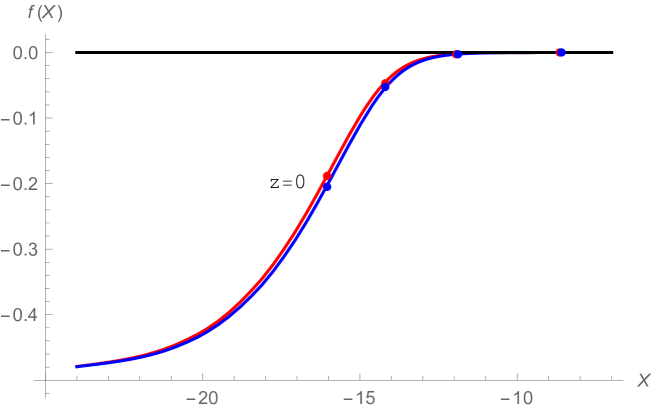
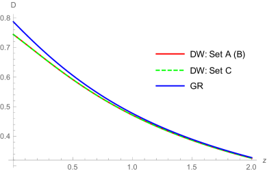
where . Reference NCA-2017 takes the analytic function (23) derived in Ref. DW-2009 (which was for ) and uses for the rest of the computations, which can be justified because the two resulting ’s are actually very close to each other, as can be seen in Fig. 1. However, it should be noted that their values at are different by at , and the difference between the growth functions for the DW model and GR is about at (see Fig. 2). Thus, for precision tests and also for consistency, one should fix according to the chosen expansion history.
III Perturbation Equations
We take scalar perturbations around the background FLRW metric in the Newtonian gauge,
| (25) |
Plugging the perturbed metric (25) into the field equations (2) and expanding them to the first order gives the perturbation equations. We symbolically write the perturbation equations as
| (26) |
In our notation, little refers to first-order perturbations, and capital to the nonlocal corrections to the original Einstein tensor. Working in Fourier space, the Einstein tensor at first order is
| (27) | |||||
| (28) |
The modified Einstein tensor at first order is
| (29) | |||||
| (30) |
Here the and components of the operator defined in (11) are
| (31) | |||||
| (32) | |||||
| (33) | |||||
| (34) | |||||
In the derivation of , the terms containing spatial derivatives have been dropped because they vanish when acting on zeroth-order values (which are functions of time only):
| (35) | |||||
| (36) | |||||
| (37) |
We also need the expansions for and at first order in and . First, can be expanded as
| (38) |
To get recall that
| (39) |
which leads to
| (40) |
Here, since and are already at first order, at first order becomes
| (41) |
In the same way, at first order is
| (42) |
In the localized formulation, the differential equations (9) and (10) for and can be expanded as
| (43) | |||||
| (44) |
These local auxiliary equations at first order are equivalent to the corresponding nonlocal expressions (41) and (42), as they should be,
| (45) | |||||
| (46) |
This fulfills the linear perturbation equations (26) for the gravitational potentials and with all the components , and and the two auxiliary equations for and given above. For the equations, contracting with the projector operator greatly simplifies them by extracting the longitudinal traceless component,
| (47) |
where represents the anisotropic stress in the convention of Ref. Ma-Bert1995 . The linear perturbation equations for and are then explicitly written as
| (48) | |||||
where and is the matter overdensity, and
| (49) |
So far, we have not taken any approximations yet, and thus these two equations (48) and (49) are full linear perturbation equations, which we have not provided in our previous papers PD-2012 ; DP-2013 . 555Equation (3.8) of Ref. NCA-2017 corresponds to (48); however, the authors omitted some terms in the sub-horizon limit. This limit will be discussed in the next subsection. Equation (3.17) of Ref. NCA-2017 is the same as (49).
At late times, which is the regime in which we are interested, the contributions to the energy from relativistic particles are negligible, and hence we can set :
| (50) |
We now have four equations for five unknown variables , and ; thus we need one more equation to complete the set of equations. It can be supplied by the energy-momentum conservation (), which is guaranteed by the conservation of the modified Einstein tensor ().
In the next subsection, we will take the sub-horizon limit () since these are the scales most relevant to structure formation and then solve those five equations. However, we must emphasize here that those equations can be solved numerically without taking any approximation. Taking the sub-horizon limit makes the equations simpler, and the solutions of the full linear equations and those of the sub-horizon limit equations have a negligible difference (for instance, in the scales of , the difference is order of ), which justifies taking the limit. However, there are important subtleties to be considered when taking this limit, which we will discuss next in detail.
III.1 Sub-horizon limit
An additional advantage of taking the sub-horizon limit is that Green’s function for the differential operator in the two auxiliary equations (45) and (46) has an analytic solution in that limit. The retarded Green’s function for the operator satisfies
| (51) |
This Green’s function can be constructed using the massless, minimally coupled scalar mode functions :
| (52) |
There is no general solution for an arbitrary , so one numerically solves for . However, for the case of sub-horizon modes (), we can find an analytic form for using the Wentzel-Kramers-Brillouin (WKB) approximation,
| (53) |
Plugging these mode functions into (52) leads to the Fourier space Green’s function,
| (54) |
The two auxiliary equations, (45) and (46) can then be solved as
| (55) | |||
| (56) |
Now, we take the sub-horizon limit, which practically means dropping time derivative terms (hence not having ) because they are a factor of smaller than the terms having in the scales of . In this limit, the equation (48) becomes the so-called modified Poisson equation,
| (57) |
The energy-momentum conservation leads to
| (58) |
which is also derived in most cosmology textbooks (see, for example, Refs. Dodelson-book and Amendola-Tsujikawa-book ). Note that in this equation for the sub-horizon limit is taken only on the rhs. We do not drop the time derivatives of on the lhs because we are eventually interested in the time evolution of . This also indicates the different nature of the gravitational potentials and from that of the matter density field . The gravitational potentials, which are parts of metric perturbations governing the geometry of the Universe, do not change much in the sub-horizon scale (while still in the linear regime). This is indeed the reason why we can safely drop the time derivatives of and and why the sub-horizon limit is also called the quasi-static limit. However, as one can see from (58), the gravitational potentials source the matter density to grow.
How about the auxiliary fields and ? The authors of Ref. NCA-2017 dropped their time derivatives, assuming they are slowly varying in the sub-horizon scale. However, the authors of Ref. DP-2013 did not drop all of their time derivatives because these fields were newly introduced variables in the DW model and their dynamics were unknown. In fact, the structure of the auxiliary equations is very similar to that of the equation for :
| (59) | |||||
| (60) | |||||
| (61) |
In all three equations, the gravitational potentials and source the time evolution of , and . As can be seen from Eq. (58), one takes the quasi-static limit (i.e., dropping times derivatives) for the source term on the right-hand side when interested in the dynamics of the variable on the left-hand side. The authors of Ref. DP-2013 followed this approach because they were interested in the dynamics of the nonlocal pieces and . The objective of their study after all was to find out how the nonlocal modification (which is encoded in and ) affects geometry and eventually matter.
Taking the sub-horizon limit in the source term of the auxiliary field equations leads to
| (62) | |||||
| (63) |
Here, from Eq. (37) and the second term of (which is ) drop in the sub-horizon limit. Then, the auxiliary equations simply become
| (64) | |||||
| (65) |
Instead, if the quasi-static limit had also been taken on the left-hand side, they would have become
| (66) | |||||
| (67) |
which are exactly the same as Eqs. (3.19) and (3.20) in Ref. NCA-2017 . It should be noted that and are now local in this implementation of the quasi-static limit. We recall that was originally nonlocal, as one can see from , and this is why the DW model is called nonlocal. This is another reason why the authors of Ref. DP-2013 were reluctant to drop the time derivatives of .
In summary, we have a system of five equations for five perturbation variables, , and in the localized formulation:
| (68) | |||||
| (69) | |||||
| (70) | |||||
| (71) | |||||
| (72) |
Or, equivalently, inserting the integral solutions for and ,
| (73) | |||||
| (74) |
leads to a system of three equations for three variables , and :
| (75) | |||||
| (76) | |||||
| (77) |
which was used by the authors of Ref. DP-2013 . As long as the initial conditions are taken the same, these two sets of equations should give the same answers for and , respectively.
III.2 Solutions of the three sets of perturbation equations
To compare with the results in Ref. NCA-2017 , we solve the three sets of perturbation equations:
- •
- •
- •
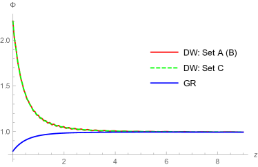
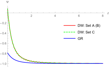
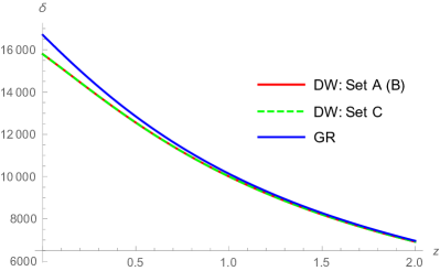
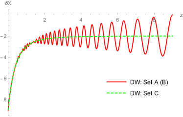
Set A and Set B give identical solutions for , and , as they should. Setting initial conditions at the same as in GR (because the nonlocal modification is negligible at , as can be seen from Fig. 1),
| (78) | |||||
| (79) | |||||
| (80) |
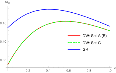
with , we have numerical solutions666 Set A can be solved using a Mathematica function NDSolve. For set B we discretized the equations and iterated them times. While the running time of set A is a few minutes, it takes set B about 11 hours with a relatively new computer. Back in 2013, running set B took days, so the current author made a simplification (a sort of localization) in which she made a coding mistake, which led to the result that now turns out to be wrong, namely, the enhanced growth of . plotted in red in Fig. 2. Their numerical values have so little difference that the two pairs of graphs from set A and set B look identical. Thus, we only provide the plots for the solutions of set A.
It should be noted that and are forced (and lightly damped) harmonic oscillators with the driving forces and for and , respectively, so that they will eventually follow the driving forces after transient oscillations. These driving forces are actually the solutions of and in (66) and (67) taken by Ref. NCA-2017 , and this is why the solutions of set C are asymptotically the same as the ones of set A (and set B). This behavior is verified in Fig. 2, which plots the solutions of set A, set C, and GR for comparison. Because is multiplied by (which is almost zero at high redshifts ) in Eqs. (68) and (69), its oscillation is killed at high redshifts. Hence, the solutions for , and of sets A and C are almost the same. As pointed out in Ref. NCA-2017 , the growth of in the DW model is lower than in GR. In Fig. 2, we also provide the normalized solution for , the growth function , which can be obtained by
| (81) |
or, equivalently, by solving the growth equation (89) given in the next subsection with the same initial conditions as in Ref. NCA-2017 :
| (82) |
 |
 |
 |
 |
 |
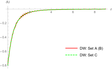 |
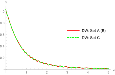
Figure 3 depicts the gravitational slip and the growth rate , which are in fair agreement with the ones obtained in Ref. NCA-2017 . The slight difference in the numerical values of in Fig. 3 and in Fig. 1 of Ref. NCA-2017 might be due to their different choices of the nonlocal distortion function (which cause their background solutions for and , and hence and , to differ slightly from the ones in this manuscript) and different values. The normalization condition for is taken to be the one given in Ref. DP-2013 , which is setting the initial amplitude the same for GR, i.e., . Reference NCA-2017 used a slightly different normalization condition that also sets the initial amplitude identical to GR but evolves it with the solution for of the DW model. Also, while we set according to the Planck 2015 results Planck2015-XIII , Ref. NCA-2017 sets .
 |
 |
III.3 Alternative definitions of the effective gravitational constant
One confusion between Refs. DP-2013 and NCA-2017 regarding the modified strength of gravity might arise from the alternative definitions of the effective gravitational constant (in units of ). In Ref. DP-2013 , it was defined through the relation between and (the modified Poisson equation), whereas in Ref. NCA-2017 , it was defined through the relation between and :
| (83) |
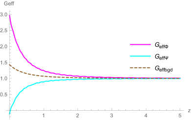
If the gravitational slip vanished (at late times) like in GR, these two definitions would be identical; however, it is not the case of the DW nonlocal model. In fact, these two ’s behave in opposite ways. While increases with time, decreases. That is, while in the DW model becomes larger than in GR, becomes smaller. This is in contrast to the case of GR in which . Another way to see the difference is that while corresponds to in the background level, more directly characterizes the growth of .
In the background level, what the DW model essentially does is increase in order to overcome the falling-down matter density . This can be seen from the Friedmann equation without :
| (84) |
The problem is that, while the left-hand side is observed to be approaching a constant, the matter density in the right-hand side is dropping as . The DW model modifies the Friedmann equation, thereby increasing the gravitational constant so that the left- and right-hand sides match each other:
| (85) |
The left panel of Fig. 4 depicts , and ( in the background level), where is obtained from by taking the background modifications only,
| (86) |
Finally, the growth equation governing the evolution of can be directly characterized by ,
| (87) |
Alternatively, using the parameter defined in Ref. def-of-mu ,
| (88) |
we have
| (89) |
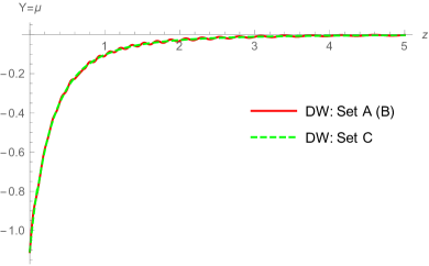
By comparing (87) and (89), one can easily see that . The right panel of Fig. 4 presents as a function of redshift, which agrees with in Ref. NCA-2017 . The sign of being negative means that the growth of gets suppressed in the DW model compared to the one in GR. Reference NCA-2017 has pointed out that this being negative is related to the violation of the ghost-free condition in the localized version ghost-nonlocal-Koivisto-0807 ; ghost-nonlocal-NOSZ-1010 ; Bamba-1104 ; ghost-nonlocal-ZS-1108 ; ghost-Amendola-0409 . 777It should be noted that Ref. NCA-2017 checked the violation of the ghost-free condition with only the background solutions and . It would be interesting to check the condition including linear perturbations, which would require solving the full linear perturbation equations. On the other hand, Refs. W-review-2014 ; DW-2013 have shown the absence of ghosts in the original nonlocal version. In any case, at the linear perturbation level, the nonlocal and localized versions give the same solutions for perturbation variables as long as the initial conditions are set the same, and no kinetic instability is observed (i.e., no linear perturbations blow up).
 |
 |
IV Discussion
We have investigated the origin of two opposite results for the growth rate in the DW nonlocal gravity model. The growth rate obtained by one group DP-2013 was higher than that of CDM, but the one obtained by the other group NCA-2017 was lower than CDM.
The evolution equations for the perturbation variables , and derived by the two groups (the former in the original nonlocal formulation and the latter in a localized version) were equivalent, and the only difference was in the implementation of the sub-horizon limit on the two auxiliary equations for and . In the sub-horizon scales of , time derivatives are typically dropped; hence, the limit is also called the quasi-static limit. While the former group took the quasi-static limit only on the source terms of the rhs to keep the time derivatives of and ,
the latter took the limit both on the lhs and rhs, which turned the differential equations into algebraic ones:
The current author initially suspected that this different implementation of the quasi-static limit was the main source of the discrepancy. However, as one can see from their equations, the auxiliary fields are forced harmonic oscillators; henceforth, they eventually follow the applied force on the source term. Moreover, the transient oscillation of in the beginning (at high redshifts) is erased by the factor of (which is almost zero at high redshifts ) in the equations of and , and therefore the two implementations give almost the same solutions for and . Working on the nonlocal form only, the author did not realize this now-simple behavior, and she made a mistake in the numerical calculation code, which unfortunately led to the result opposite of the one by Ref. NCA-2017 .
We summarize what should be corrected in our previous papers PD-2012 ; DP-2013 ; PS-2016 . In Ref. PD-2012 , all equations and the numerical results plotted in figures are actually correct. However, it should be noted that the results of and were obtained by solving the perturbation equations perturbatively, which means by inserting the standard CDM solution for and into the new terms. Since and in the DW model turn out to be quite different from and , these are somewhat rough estimates. In Ref. DP-2013 , all equations are correct, but the numerical solutions plotted in the figures are wrong; therefore, the discussions based on those solutions should be discarded. Reference PS-2016 attempted to lower the growth of by changing the background expansion rather than that of CDM, motivated by the wrong conclusion of Ref. DP-2013 that the DW model cannot do better than CDM in suppressing growth when its background is fixed by CDM. All equations there are also correct, but the solutions for plotted in Figs. 2 and 3 are subject to change. The tendency that the equation of state less negative than gives more suppressed growth might still remain because the dimensionless Hubble parameter being in the denominator in the source term of the growth equation ((17) in Ref. PS-2016 ) was a key factor lowering the growth. However, more careful analysis is required to confirm it. Furthermore, it would be still worth it to check the growth of perturbations in the DW model with different background expansions rather than CDM.
After all, we extend the conclusion of Ref. NCA-2017 to include the equivalence of the nonlocal and localized formulations on the linear perturbation level so that both versions of the DW model make identical predictions: the lower growth of the matter overdensity compared to the case of CDM. We also remark that the entire analysis on the perturbation equations in this paper was performed for only one scale and the quasi-static approximation worked very well in this sub-horizon scale. This raises the question of in what range of the approximation holds. Solving the full linear perturbation equations without taking the quasi-static limit would help to answer this question. We note that the full linear equations for and are already given in (48) and (49), and for , and , we only need to recover the time derivatives dropped in the source terms. It would be also interesting to check the dependence of the solutions on the initial conditions. In practice, the localized version is much simpler than the nonlocal one and is expected to be relatively easily incorporated with extensive cosmological simulation codes such as CAMB CAMB and CLASS CLASS . There are also theoretical issues like the apparent violation of the ghost-free condition in the localized formulation. However, we agree with the authors of Ref. NCA-2017 that the DW nonlocal model gives interesting predictions at linear perturbation level and deserves further consideration.
Acknowledgements
The author is grateful to Luca Amendola, Adrian Fernandez Cid, and Henrik Nersisyan for bringing the discrepancy to her attention and for the helpful discussions. The author also thanks Sibel Boran, Scott Dodelson, Emre Onur Kahya, Stéphane Ilić, Arman Shafieloo, Constantinos Skordis, and Richard Paul Woodard for their insightful comments. The research leading to these results has received funding from the European Research Council under the European Union’s Seventh Framework Programme (FP7/2007-2013) / ERC Grant No. 617656, “Theories and Models of the Dark Sector: Dark Matter, Dark Energy and Gravity.”
References
- [1] S. Deser and R. P. Woodard, Phys. Rev. Lett. 99, 111301 (2007), arXiv:0706.2151.
- [2] L. Joukovskaya, Phys. Rev. D 76, 105007 (2007), arXiv:0707.1545.
- [3] S. Nojiri and S. D. Odintsov Phys. Lett. B 659, 821 (2008), arXiv:0708.0924.
- [4] G. Calcagni, M. Montobbio and G. Nardelli, Phys. Lett. B 662, 285 (2008), arXiv:0712.2237.
- [5] S. Jhingan, S. Nojiri, S. D. Odintsov, M. Sami, I. Thongkool and S. Zerbini, Phys. Lett. B 663, 424 (2008), arXiv:0803.2613.
- [6] T. S. Koivisto, Phys. Rev. D 77, 123513 (2008), arXiv:0803.3399.
- [7] T. S. Koivisto, Phys. Rev. D 78, 123505 (2008), arXiv:0807.3778.
- [8] S. Capozziello, E. Elizalde, S. Nojiri and S. D. Odintsov, Phys. Lett. B 671, 193 (2009), arXiv:0809.1535.
- [9] N. A. Koshelev, Grav. Cosmol. 15, 220 (2009), arXiv:0809.4927.
- [10] C. Deffayet and R. P. Woodard, J. Cosmol. Astropart. Phys. 08 (2009) 023, arXiv:0904.0961.
- [11] T. Biswas, T. S. Koivisto and A. Mazumdar, J. Cosmol. Astropart. Phys. 11 (2010) 008, arXiv:1005.0590.
- [12] S. Nojiri, S. D. Odintsov, M. Sasaki and Y.-l. Zhang, Phys. Lett. B 696, 278 (2011), arXiv:1010.5375.
- [13] K. Bamba, S. Nojiri, S. D. Odintsov, and M. Sasaki, Gen. Rel. Grav. 44, 1321 (2012), arXiv:1104.2692.
- [14] A. O. Barvinsky, Phys. Lett. B 710, 12 (2012), arXiv:1107.1463.
- [15] Y.-l. Zhang and M. Sasaki, Int. J. Mod. Phys. D 21, 1250006 (2012), arXiv:1108.2112.
- [16] E. Elizalde, E. O. Pozdeeva and S. Yu. Vernov, Phys. Rev. D 85, 044002 (2012), arXiv:1110.5806.
- [17] A.O. Barvinsky, Phys. Rev. D 85, 104018 (2012), arXiv:1112.4340.
- [18] S. Park and S. Dodelson, Phys. Rev. D 87, 024003 (2013), arXiv:1209.0836.
- [19] A. O. Barvinsky and Y. V. Gusev, Phys. Part. Nucl. 44, 213 (2013), arXiv:1209.3062.
- [20] E. Elizalde, E. O. Pozdeeva and S. Yu. Vernov, Class. Quant. Grav. 30, 035002 (2013), arXiv:1209.5957.
- [21] E. Elizalde, E. O. Pozdeeva, S. Yu. Vernov and Y.-l. Zhang, J. Cosmol. Astropart. Phys. 07 (2013) 034, arXiv:1302.4330.
- [22] M. Maggiore, Phys. Rev. D 89, 043008 (2014), arXiv:1307.3898.
- [23] S. Deser and R. P. Woodard, J. Cosmol. Astropart. Phys. 11 (2013) 036, arXiv:1307.6639.
- [24] S. Dodelson and S. Park, Phys. Rev. D 90, 043535 (2014), arXiv:1310.4329.
- [25] S. Foffa, M. Maggiore, and E. Mitsou, Phys. Lett. B 733, 76 (2014), arXiv:1311.3421.
- [26] S. Foffa, M. Maggiore, and E. Mitsou, Int. J. Mod. Phys. A 29, 1450116 (2014), arXiv:1311.3435.
- [27] R. P. Woodard, Found. Phys. 44, 213 (2014), arXiv:1401.0254.
- [28] A. Kehagias and M. Maggiore, J. High Energy Phys. 08 (2014) 029, arXiv:1401.8289.
- [29] M. Maggiore and M. Mancarella, Phys. Rev. D 90, 023005 (2014), arXiv: 1402.0448.
- [30] Y. Dirian, S. Foffa, N. Khosravi, M. Kunz, and M. Maggiore, J. Cosmol. Astropart. Phys. 06 (2014) 033, arXiv:1403.6068.
- [31] A. Conroy, T. Koivisto, A. Mazumdar, and A. Teimouri, Class. Quant. Grav. 32, 015024 (2015), arXiv:1406.4998.
- [32] A. Barreira, B. Li, W. A. Hellwing, C. M. Baugh, and S. Pascoli, J. Cosmol. Astropart. Phys. 09 (2014) 031, arXiv:1408.1084.
- [33] Y. Dirian and E. Mitsou, JCAP 1410 (2014) 065, arXiv:1408.5058.
- [34] Y. Dirian, S. Foffa, M. Kunz, M. Maggiore, and V. Pettorino, J. Cosmol. Astropart. Phys. 04 (2015) 044, arXiv:1411.7692.
- [35] X. Zhang, Y. Wu, S. Li, Y. Liu, B. Chen, Y. Chai, and S. Shu, J. Cosmol. Astropart. Phys. 07 (2016) 003, arXiv:1511.05238.
- [36] G. Cusin, S. Foffa, M. Maggiore, and M. Mancarella, Phys. Rev. D 93 (2016) 043006, arXiv:1512.06373.
- [37] Y.-l. Zhang, K. Koyama, M. Sasaki, and G. Zhao, J. High Energy Phys. 03 (2016) 039, arXiv:1601.03808.
- [38] G. Cusin, S. Foffa, M. Maggiore, and M. Mancarella, Phys. Rev. D 93, 083008 (2016), arXiv:1602.01078.
- [39] Y. Dirian, S. Foffa, M. Kunz, M. Maggiore, and V. Pettorino, J. Cosmol. Astropart. Phys. 05 (2016) 068, arXiv:1602.03558.
- [40] M. Maggiore, Phys. Rev. D 93, 063008 (2016), arXiv:1603.01515.
- [41] H. Nersisyan, Y. Akrami, L. Amendola, T. S. Koivisto, and J. Rubio, Phys. Rev. D 94, 043531 (2016), arXiv:1606.04349.
- [42] M. Maggiore, Fundam. Theor. Phys. 187, 221 (2017), arXiv:1606.08784.
- [43] S. Park and A. Shafieloo, Phys. Rev. D 95, 064061 (2017), arXiv:1608.02541.
- [44] Y. Wu, X. Zhang, M. Wu, N. Zhang, and B. Chen, Chin. Phys. Lett. 34, 079801 (2017), arXiv:1611.07209.
- [45] H. Nersisyan, A. F. Cid, and L. Amendola, J. Cosmol. Astropart. Phys. 04 (2017) 046, arXiv:1701.00434.
- [46] I. Dimitrijevic, B. Dragovich, J. Stankovic, A. S. Koshelev, and Z. Rakic, Springer Proc. Math. Stat. 191, 35 (2016), arXiv:1701.02090.
- [47] V. Vardanyan, Y. Akrami, L. Amendola, and A. Silvestri, arXiv:1702.08908.
- [48] Y. Dirian, Phys. Rev. D 96, 083513 (2017), arXiv:1704.04075.
- [49] L. Amendola, N. Burzilla, and H. Nersisyan, Phys. Rev. D 96, 084031 (2017), arXiv:1707.04628.
- [50] K.Y. Roobiat and R. Pazhouhesh, Int. J. Mod. Phys. D 26, 1750134 (2017).
- [51] X. Zhang, Y. Wu, W. Yang, C. Zhang, B. Chen, and N. Zhang, Sci. China Phys. Mech. Astron. 60, 100411 (2017).
- [52] S. Bahamonde, S. Capozziello, and K. F. Dialektopoulos, Eur. Phys. J. C 77, 722 (2017), arXiv:1708.06310.
- [53] S. Bahamonde, S. Capozziello, M. Faizal, and R. C. Nunes, Eur. Phys. J. C 77, 628 (2017), arXiv:1709.02692.
- [54] K. Bamba, D. Momeni, and M. A. Ajmi, arXiv:1711.10475.
- [55] L. Parker and D. J. Toms, Phys. Rev. D 32, 1409 (1985).
- [56] T. Banks, Nucl. Phys. B 309, 493 (1988).
- [57] C. Wetterich, Gen. Rel. Grav. 30, 159 (1998), gr-qc/9704052.
- [58] A. O. Barvinsky, Phys. Lett. B 572, 109 (2003), hep-th/0304229.
- [59] H. W. Hamber and R. M. Williams, Phys. Rev. D 72, 044026 (2005), hep-th/0507017.
- [60] T. Biswas, A. Mazumdar, and W. Siegel, J. Cosmol. Astropart. Phys. 03 (2006) 009, hep-th/0508194.
- [61] D. Lopez Nacir and F. D. Mazzitelli, Phys. Rev. D 75, 024003 (2007), hep-th/0610031.
- [62] P. G. Ferreira and A. L. Maroto, Phys. Rev. D 88, 123502 (2013), arXiv:1310.1238.
- [63] J. F. Donoghue and B. K. El-Menoufi, Phys. Rev. D 89, 104062 (2014), arXiv:1402.3252.
- [64] X. Calmet, D. Croon, and C. Fritz, Eur. Phys. J. C 75, 605 (2015), arXiv:1505.04517.
- [65] J. F. Donoghue and B. K. El-Menoufi, J. High Energy Phys. 10 (2015) 044, arXiv:1507.06321.
- [66] I. Oda, Phys. Rev. D 95, 104020 (2017), arXiv:1704.05619.
- [67] I. Oda, Phys. Rev. D 96, 024027 (2017), arXiv:1706.01683.
- [68] I. Oda, arXiv:1709.08189.
- [69] M. Elias, F. D. Mazzitelli, and L.G. Trombetta, Phys. Rev. D 96, 105007 (2017), arXiv:1709.10435.
- [70] T. Bautista, A. Benevides, and A. Dabholkar, arXiv:1711.00135.
- [71] S. O. Alexeyev, X. Calmet, and B. N. Latosh, Phys. Lett. B 776, 111 (2018), arXiv:1711.06085.
- [72] I. Oda, arXiv:1711.10476.
- [73] N. C. Tsamis and R. P. Woodard, Phys. Rev. D 80, 083512 (2009), arXiv:0904.2368.
- [74] N. C. Tsamis and R. P. Woodard, Phys. Rev. D 82, 063502 (2010), arXiv:1006.4834.
- [75] N. C. Tsamis and R. P. Woodard, J. Cosmol. Astropart. Phys. 09 (2014) 008, arXiv:1405.4470.
- [76] A. S. Koshelev, K. S. Kumar, and P. V. Moniz, Phys. Rev. D 96, 103503 (2017), arXiv:1604.01440.
- [77] N. C. Tsamis and R. P. Woodard, Phys. Rev. D 94, 043508 (2016), arXiv:1606.06967.
- [78] M. E. Soussa and R. P. Woodard, Class. Quant. Grav. 20, 2737 (2003), astro-ph/0302030.
- [79] C. Deffayet, G. Esposito-Farese, and R. P. Woodard, Phys. Rev. D 84, 124054 (2011), arXiv:1106.4984.
- [80] R. P. Woodard, Can. J. Phys. 93, 242 (2015), arXiv:1403.6763.
- [81] C. Deffayet, G. Esposito-Farese, and R. P. Woodard, Phys. Rev. D 90, 064038 (2014), Addendum: Phys.Rev. D 90, 089901 (2014), arXiv:1405.0393
- [82] M. Kim, M.H. Rahat, M. Sayeb, L. Tan, R. P. Woodard, and B. Xu, Phys. Rev. D 94, 104009 (2016), arXiv:1608.07858.
- [83] E. Bertschinger, Astrophys. J. 648, 797 (2006), astro-ph/0604485.
- [84] W. Hu and I. Sawicki, Phys. Rev. D 76, 104043 (2007), arXiv:0708.1190.
- [85] T. Baker, P. G. Ferreira, and C. Skordis, Phys. Rev. D 87, 024015 (2013), arXiv:1209.2117.
- [86] D. Huterer, D. Kirkby, R. Bean, A. Connolly, K. Dawson, et al., Astropart. Phys. 63, 23 (2015), arXiv:1309.5385.
- [87] J. Dunkley et al. [WMAP Collaboration], Astrophys. J. Suppl. 180, 306 (2009), arXiv:0803.0586. E. Komatsu et al. [WMAP Collaboration], Astrophys. J. Suppl. 180, 330 (2009), arXiv:0803.0547.
- [88] Planck Collaboration, Astron. Astrophys. 594, A13 (2015), arXiv:1502.01589.
- [89] C.-P. Ma and E. Bertschinger, Astrophys. J. 455, 7 (1995), arXiv:astro-ph/9506072.
- [90] S. Dodelson, Modern Cosmology (Academic Press, San Diego, 2003).
- [91] L. Amendola and S. Tsujikawa, Dark Energy: Theory and Observations (Cambridge University Press, 2010).
- [92] F. Simpson, C. Heymans, D. Parkinson, C. Blake, M. Kilbinger, et al., Mon. Not. Roy. Astron. Soc. 429, 2249 (2013), arXiv:1212.3339.
- [93] L. Amendola, Phys. Rev. Lett. 93, 181102 (2004), hep-th/0409224.
- [94] A. Lewis and A. Challinor, CAMB: Code for Anisotropies in the Microwave Background, Astrophysics Source Code Library (2011), ascl:1102.026.
- [95] D. Blas, J. Lesgourgues, and T. Tram, JCAP 07 (2011) 034, arXiv:1104.2933.