Thermal dynamics of lattice modes near a polaronic crossover:
from the dilute polaron limit to a charge ordered state

Abstract

We provide a comprehensive solution to the lattice dynamics problem in the two dimensional Holstein model at finite electron density and finite temperature. We work in the physically relevant adiabatic regime and vary the electron-phonon interaction from the weak coupling perturbative window to the strong coupling polaronic regime. We explore three typical electron densities, dilute - where spatial correlations between polarons is weak, intermediate - where correlations are significant, and half-filling - where there is long range checkerboard order at low temperature. We use two methods both of which exploit the “slowness” of the phonons to handle the problem. These are (i) a standard random phase approximation (RPA), adapted to capture small quantum fluctuations on Monte Carlo generated classical thermal backgrounds, and (ii) a Langevin dynamics scheme, with a simplified “thermal noise”, that can address large amplitude dynamical fluctuations. The Langevin scheme, as we argue in the paper, is the superior method in the strong coupling part of the phase diagram, where lattice distortions are large. It reveals a non trivial multi-peak momentum resolved spectrum with a high energy part, on the scale of the bare phonon frequency $\Omega$, and a low energy peak at $\omega\ll\Omega$. Below the polaronic threshold, the high energy dispersion changes only modestly with temperature $T$, while the broadening, arising from mode coupling, increases linearly with $T$ at low temperature. The low energy peak shows up at strong coupling and finite temperature and arises from the slow tunneling of polarons. The tunneling events become spatially correlated as electron density increases towards half-filling, and the weight becomes strongly momentum and temperature dependent. We suggest the analytic basis of these results.

I Introduction

Strong electron-phonon interaction is a crucial ingredient in the physics of many functional materialspol1 . Among these are phonon mediated superconductors like alkali doped fulleridesfullerides , BiO based compoundsBiO , the colossal magnetoresistance manganitesCMR ; man , and possibly even the cuprates cpr1 ; cpr2 . The presence of strong electron-phonon (EP) coupling is suggested in some cases by mid-infrared absorption fullerides ; BiO and in some others by neutron scattering cpr1 ; cpr2 ; weber1 ; weber2 ; weber3 ; weber4 ; kajimoto ; reznik ; dean ; braden .

Strong EP interaction leaves an imprint on the phonon spectrum. In some metallic manganites, near a short-range charge ordered (CO) insulator weber1 ; weber2 ; weber3 ; weber4 , one observes anomalous broadening and softening of bond-stretching phonons. Similar softening and band-splitting have been reported in doped nickelateskajimoto near a checkerboard ordered phase. In cuprates phonons are strongly affected reznik for momenta close to the wavevector of stripe order, and recent experiments reveal a non-trivial temperature dependence of the softening wavevector dean . Finally, giant phonon anomalies have been observed in doped bismuthates braden . The effects above trace back to polaronic correlations in these materials.

Polarons form as a bound state between an electron and a phonon cloud when the EP coupling exceeds a threshold. Theoretical problems in polaron physics are broadly to (a) understand the ‘single polaron’ problem, (b) address collective effects, e.g, ordering tendencies and spatial correlations among the polarons, (c) probe the spectral and conducting properties of the polaron fluid, and (d) clarify the impact of polaron formation and CO correlations on the phonon dynamics. (a)-(c) are reasonably well studied var ; diag1 ; diag2 ; inst ; berciu ; zeyher ; millis1 ; millis2 ; ciuchi1 ; ciuchi2 ; kumar1 , (d), our focus, much less so. The focus of this paper is on phonon dynamics in electron-phonon systems when there are either large thermally induced distortions in a metal close to a polaronic crossover or there are polaronic distortions in the ground state itself. In both these cases polaron tunneling leads to a highly anharmonic signature in the dynamics. Before discussing issues in phonon dynamics we quickly recapitulate the key results on (a)-(c) to set the background.

The single polaron problem is essentially understood, via a combination of variational techniquesvar - which yields ground state energies, polaron bandwidth, and electron effective mass, numerical diagonalizationdiag1 ; diag2 , and instanton methodsinst . The recently developed ‘momentum averaged’ approximationberciu yields accurate spectral function in this problem. The traditional tool at finite density is Migdal-Eliashberg (ME) theory ME theory but it cannot access polaron physics. To overcome this other approaches like adiabatic expansion zeyher ; millis1 ; millis2 , or numerical schemes like quantum Monte Carlo QMC (QMC) and dynamical mean field theory DMFT (DMFT) have been developed. DMFT suggests crossover from polaronic quasparticles at low temperature to an incoherent high temperature phase ciuchi1 at low density, and a metal-insulator transition at half-filling ciuchi2 . In the strict adiabatic limit the ground state in two and three dimensions has also been established kumar1 .

The phonon physics is relatively less explored. QMC investigations indicate the opening of a Peierls gap in the strong coupling spinless 1D model creff , and have probed the effect of Peierls transition on the dynamical structure factor hohen . DMFT suggests phonon softening bulla at strong coupling, but misses the momentum dependence of phonon broadening and the connection between phonon dynamics and short-range static correlations. There are analytical studies at low filling fehske in 1D and numerics at relatively weak coupling hague in 2D, yielding phonon dispersion and self-energies. Recently scalettar the role of ‘bare’ phonon dispersion in deciding charge density wave and superconducting transitions has been probed.

The situations where the phonon dynamics remains poorly understood are- (i) there are large thermally induced distortions in a metal close to a polaronic crossover, (ii) there are polaronic distortions in the ground state itself and the polarons undergo tunneling, and (iii) there are significant short range charge ordering correlations.

We address phonon dynamics in the context of the two dimensional Holstein model. We use methods that are formulated in real space, to capture spatial correlations, and real frequency (or real time). The methods are described in detail later, at the moment we just state that these are (a) the random phase approximation (RPA) applied on classical thermal backgrounds generated via a ‘static path approximation’ (SPA) Monte Carlo (MC) strategy kumar1 , and (b) a dynamical approach involving a Langevin equation driven by thermal noise chern ; sauri . The RPA sets a reference because of its wide use in the community but we discover that in the strong coupling regime the Langevin dynamics (LD) results capture the physics far better.

The parameter space of our problem includes (i) the ratio $\gamma$ of the phonon frequency $\Omega$ to electron hopping (indicating the degree of ‘adiabaticity’), (ii) the ratio $\lambda$ of ‘polaron binding energy’ $E_{p}$ to half of the electron bandwidth $W/2$, (iii) the electron density $n$, and (iv) the temperature $T$. We focus on the adiabatic regime, $\Omega/t\ll 1$, and provide detailed phonon spectra over the $\lambda-T$ parameter space at three typical densities: (a) $n=0.1$, where spatial correlations amongst polarons are weak, (b) $n=0.4$, where charge correlations are significant, and (c) $n=0.5$, where the system has a charge ordered ground state.

While the results in the paper are organised in terms of the three density regimes above, a classification in terms of the dynamical regimes we observe is more compact. The relevant parameters for this are (i) the strength of coupling $\lambda$ with respect to the coupling $\lambda_{c}(n)$ for the polaronic transition in the ground state, and (ii) the proximity of the density to half-filling, $n=0.5$ (where a CO state occurs). We denote the characteristic scale of polaronic distortion as $x_{pol}\sim\sqrt{8\lambda t/K}$. In terms of these our main results are below.

1. We observe three broad dynamical regimes - (a) perturbative, (b) polaron tunneling, and (c) large oscillations. Regime (a) involves small oscillations, $\Delta x\ll x_{pol}$, about homogeneous backgrounds, accessible through both RPA and LD methods. Regimes (b) and (c) involve ‘large amplitude’ dynamics, where $\Delta x\gtrsim x_{pol}$. These are inaccessible within the RPA scheme.

2. In the polaron tunneling regime the time series consists of small oscillations, with amplitude $\Delta x\ll x_{pol}$, with occasional large moves, $\Delta x\sim x_{pol}$. In the large oscillation regime there is a continuum of fluctuation going even beyond $x_{pol}$. The power spectrum in the tunneling regime is ‘two branch’ as opposed to a broad single branch for large oscillations.

3. (i) For $\lambda<\lambda_{c}(n)$, the low temperature dynamics is accessible within RPA and falls in regime (a) and even intermediate $T$ phonons can be described perturbatively, if one is not too close to $\lambda_{c}$. (ii) For $\lambda\sim\lambda_{c}(n)$ increasing $T$ leads to a crossover from regime (a) to regime (c). (iii) For $\lambda>\lambda_{c}(n)$, large distortions are present at $T=0$ and we observe dynamics characterized by regime (b) at low temperature, gradually crossing over to (c) with increasing $T$.

4. At half-filling $\lambda_{c}=0$ and the ground state is $(\pi,\pi)$ ordered. Here, RPA is valid over a wider region at low $T$, whose dynamics is of type (a). We see a gradual evolution from (a) to (b) to (c) on increasing $T$.

The rest of the paper is organised as follows: in Section II we discuss our model and methods. Section III provides an overview of the dynamical regimes that emerge on varying density, coupling and temperature. Section IV presents detailed results in the dilute regime, $n=0.1$. Section V shows results in the ‘charge correlated’ regime, $n=0.4$, while Section VI provides some results on the charge ordered phase at $n=0.5$. Section VII discusses the interpretation, validity, and applicability of our results. We then conclude. Some of the detailed formulae are given in an Appendix.

II Model and method

We study the single band, spinless, Holstein model on a 2D square lattice:

$$H=\sum_{<ij>}t_{ij}c^{\dagger}_{i}c_{j}+\sum_{i}(\frac{p^{2}_{i}}{2M}+\frac{1}{2}Kx^{2}_{i})-g\sum_{i}n_{i}x_{i}$$ (1)

Here, $t_{ij}$’s are the hopping amplitudes. We study a nearest neighbour model with $t=1$ for three values of density, viz. $n=0.1$, $n=0.4$ and $n=0.5$. $K$ and $M$ are the stiffness constant and mass, respectively, of the optical phonons, and $g$ is the electron-phonon coupling constant. We set $K=1$, $M$ is tuned to adjust the bare phonon frequency. The $M\rightarrow\infty$ limit for fixed $K$ is the adiabatic limit. In this paper, we report studies for $\Omega=\sqrt{K/M}=0.1$, which is a reasonable value for real materials. The chemical potential $\mu$ is varied to maintain the electron density at the required value.

II.1 Random phase approximation (RPA) at $T\neq 0$

The model above leads to the action

$$S = \int_{0}^{\beta}d\tau[\sum_{ij}\bar{\psi_{i}}\{(\partial_{\tau}-\mu)\delta_{ij}-t_{ij}\}\psi_{j}+\sum_{i}\bar{\phi_{i}}(\partial_{\tau}+\Omega)\phi_{i}$$ (3)

$$~{}~{}~{}~{}~{}~{}~{}~{}~{}~{}~{}~{}~{}~{}-~{}g\sqrt{\frac{\Omega}{2K}}\sum_{i}(\bar{\phi_{i}}+\phi_{i}){\bar{\psi}_{i}}\psi_{i}]$$

Here $\psi_{i}$ and $\phi_{i}$ are the fermion and coherent state Bose fields respectively. and $\beta$ denotes the inverse temperature and we use units where $k_{B}=1$, $\hbar=1$. The relation between the real and coherent state fields is

$$x_{i}=\sqrt{\frac{1}{2M\Omega}}(\phi_{i}+\bar{\phi}_{i})$$ (4)

In QMC QMC , one ‘integrates out’ the fermion fields to construct the effective bosonic action. The equilibrium configurations $\phi_{i}(\tau)$ of that theory are obtained via Monte Carlo sampling. Physical correlators are then computed as averages with respect to these $\phi_{i}(\tau)$ configurations. Within DMFT DMFT one maps the original action in Eq.(2) to an impurity problem, with parameters determined self-consistently.

In the adiabatic limit, i.e, a static approximation for the phonons, one treats the $x_{i}$ as classical fields, neglecting their imaginary time dependence. This corresponds to the case of infinite $M$ for a fixed $K$. The quantum character of lattice vibrations is built in perturbatively.

The full action containing the electrons and displacement fields can be rewritten in frequency space as-

$$S = S_{ph}+S_{f}$$

$$S_{ph} = \frac{1}{2}\sum_{i,m}\bar{x}_{im}(M\Omega_{m}^{2}+K)x_{im}$$ (5)

$$S_{f} = \sum_{i,j,\alpha,\beta}\bar{\psi}_{i\alpha}[(-i\omega_{\alpha}-\mu)\delta_{ij}\delta_{\alpha\beta}-t_{ij}\delta_{\alpha\beta}$$ (7)

$$~{}~{}~{}~{}~{}~{}~{}~{}~{}~{}~{}~{}~{}~{}~{}~{}~{}~{}-g\sqrt{\beta}x_{i,\alpha-\beta}\delta_{ij}]\psi_{j\beta}$$

where $\omega_{\alpha}$ and $\omega_{\beta}$ are fermionic Matsubara frequencies, $\Omega_{m}$ is a Bose frequency. To get the partition function, one integrates over $\psi_{i\alpha}$, $x_{i0}$ and the $x_{im}$ fields.

The next step is to separate the Bose field into zero and non-zero Matsubara modes. We write $S=S_{0}+S_{1}$ where the first part contains fermions coupling only to the zero frequency (static) mode and the second, the finite frequency modes. We can formally ‘diagonalize’ the fermions in presence of the static mode to write $S_{0}$ as-

$$S_{0}={\sum_{l,\alpha}\bar{\xi}_{l,\alpha}(-i\omega_{\alpha}+\epsilon_{l})\xi_{l,\alpha}}+\frac{1}{2}K\sum_{i}x^{2}_{i0}$$ (8)

where $\xi$’s correspond to the fermionic eigenmodes in the $\{x_{i0}\}$ background. $S_{0}$ defines the static path approximation (SPA) action. The eigenvalues ($\epsilon_{l}$’s ) depend non-trivially on the $\{x_{i0}\}$ background. To obtain the effective zero mode distribution $P\{x_{i0}\}$, one has to integrate out the fermions. At the SPA level, there exists an effective Hamiltonian $H_{eff}$, depending on $x_{i0}$, for the fermions and the distribution can be formally written as-

$$P\{x_{i0}\} = Tr_{c,c^{\dagger}}e^{-\beta(H_{eff}+{1\over 2}Kx_{i0}^{2})}$$ (9)

$$H_{eff} = \sum_{<ij>}t_{ij}c^{\dagger}_{i}c_{j}-g\sum_{i}n_{i}x_{i0}$$

Around the SPA action, we set up a cumulant expansion of $S_{1}$. Owing to the disparate timescales of the phonons and electrons, we attempt a sequential integrating out. First, the fermions are traced out and one obtains the following expression for $S_{1}$ in terms of the $x_{i}(i\Omega_{m})$:

$$S_{1} = S^{\prime}_{ph}-Trln[\beta((-i\omega_{\alpha}-\mu)\delta_{ij}\delta_{\alpha\beta}$$

$$~{}~{}~{}~{}~{}~{}~{}~{}~{}~{}~{}~{}~{}~{}~{}-t_{ij}\delta_{\alpha\beta}-g\sqrt{\beta}x_{i,\alpha-\beta}\delta_{ij})]$$

$$S^{\prime}_{ph} = \frac{1}{2}\sum_{i,m\neq 0}\bar{x}_{im}(M\Omega_{m}^{2}+K)x_{im}$$ (11)

Analytic determination of the trace is impossible beyond weak coupling. Our method constitutes of expanding the trace in finite frequency $x_{i}$ modes upto Gaussian level. Physically, we assume that the quantum fluctuations are small in amplitude, controlled by a low $\gamma=\Omega/t$ ratio. Retaining only quadratic terms in the dynamic modes allows us to analytically integrate them out later. The method is obviously perturbative in $\gamma$ as we diagonalize the fermions in presence of static distortions and evaluate correlation functions on this ‘frozen’ background, which enter as coefficients of the quadratic Bose term for finite frequencies. After re-exponentiating this term the new partition function becomes-

$$Z=\int[D\bar{x}][Dx][D\bar{\xi}][D\xi]e^{-(S_{0}+S_{1})}$$ (12)

where

$$S_{0} = {\sum_{l,\alpha}\bar{\xi}_{l,\alpha}(-i\omega_{\alpha}+\epsilon_{l})\xi_{l,\alpha}}+\frac{1}{2}Kx_{i0}^{2}$$ (13)

$$S_{1} = {\sum_{i,j,m>0}\bar{x}_{im}[(M\Omega^{2}_{m}+K)\delta_{ij}+{g^{2}}\Pi_{ij}^{m}(\{x_{i,0}\})]x_{jm}}$$

Here $\Pi_{ij}^{m}$ is a one-loop fermion polarization correcting the free Bose propagators. The expression for this is

$$\Pi_{ij}^{m}(\{x_{i0}\})=\frac{1}{\beta}\sum_{\alpha}G_{ij}^{\alpha}G_{ji}^{\alpha-m}$$ (14)

$G_{ij}^{\alpha}$’s are Matsubara components of real-space fermion Green’s functions computed in an arbitrary static background. One can write a spectral representation of this as follows-

$$G^{\alpha}_{ij}(\{x_{i0}\})=\sum_{n}\frac{u_{in}\bar{u}_{jn}}{i\omega_{\alpha}-\epsilon_{n}}$$ (15)

where $u_{in}$ is amplitude at site $i$ for the $n$th eigenstate of the SPA Hamiltonian and $\epsilon_{n}$’s are the corresponding eigenvalues.

The fermion diagonalization for arbitrary static distorted backgrounds has to be dealt with numerically. To access large system sizes within a reasonable simulation time, a cluster algorithm is used for each Metropolis update. The method has been extensively benchmarked earlier. kumar2 . Our studies are on 32$\times$32 lattices using 8$\times$8 clusters.

The coefficient of the quadratic Bose term of $S_{1}$ in (9) defines the inverse propagator $(D^{-1})_{ij,m}$ for the renormalized phonons. One can view the $\Pi^{m}_{ij}$ as a self-energy for the phonons in real space, correcting the bare propagator. To get the renormalized Green’s function, we solve a Dyson’s equation on the lattice with inhomogeneous backgrounds.

$$[D]^{-1}_{ij}(\omega)=[D]^{-1}_{0,ij}(\omega)+g^{2}[\Pi]_{ij}(\omega)$$ (16)

Here the bare phonon propagator $D^{-1}_{0,ij}$ is defined through the equation-

$$[D]^{-1}_{0,ij}(\omega)=(M\omega^{2}-K)\delta_{ij}$$ (17)

where we have analytically continued the Green’s functions to real frequency and $D^{-1}_{0,ij}$ denotes the inverse propagator for the bare phonon. This involves a calculation that grows as $O(N^{4})$ with increasing lattice size $N$. For lattices of size 18$\times$18, this computation was implemented.

While we used the scheme above as our benchmark, we tried out an approximation, explored earlier in the context of DMFT, where the polarization is replaced by its $\omega_{m}=0$ component for all the Bose modesmillis2 . This approximation renders a direct solution of Dyson’s equation for the phonon propagator unnecessary. Instead, to extract the renormalized spectrum, one has to solve a single Hamiltonian problem for the bosons in real space for each background configuration. The results reasonably match with full RPA in the weak and strong coupling windows, but aren’t reliable near the crossover.

On structurally disordered configurations, $\Pi_{ij}(\omega)$ is not translationally invariant. We take a Fourier transform of $D_{ij}$ with respect to ($\vec{R_{i}}-\vec{R_{j}}$), compute the phonon spectrum and finally average over equilibrium backgrounds. From this Bose propagator, we also find out the phonon density of states (DOS) by tracing over momenta. The expressions for $\Pi^{m}_{ij}$ and $D^{m}_{ij}$ in the $\omega_{m}=0$ approximation are quoted in the Appendix.

This RPA method, while being complicated in its implementation, essentially captures small amplitude quantum fluctuations about equilibriun ‘backgrounds’. Hence, it’s adequate in the low temperature, weak coupling scenario. However, one misses out on anharmonic ‘mode coupling’ physics and most importantly, thermally induced polaron tunneling. The latter involves ‘swapping’ of large distortions on neighbouring sites and are crucial in describing critical dynamics at half-filling. Even at lower densities, these moves help in cause a very interesting low-frequency weight transfer in the phonon spectrum. To capture them, we’ve used a real time equation of motion method, described next.

II.2 Langevin Dynamics (LD) method

The Holstein problem can be set up in the Keldysh language in terms of coherent state fields corresponding to $x_{i}$ and $c_{i}$ operators, with their full space-time dependence retained. We indicate how a Langevin-like equation of motion sauri can be obtained from the Keldysh action in the adiabatic limit. Physically, this corresponds to a “small $\dot{x}$” approximation- namely the velocity of this field is much smaller than Fermi velocity. We outline this below.

The partition function for the $x_{i}$ ‘oscillators’ can be written as-

$$Z_{osc}=\int Dx_{i,f}Dx_{i,r}e^{i(S_{0}+S_{1})}$$ (18)

Here $x_{i,f}$ and $x_{i,r}$ are lattice displacement fields along forward and return contours respectively. The expressions for $S_{0}$ and $S_{1}$ are-

$$S_{0} = \frac{1}{2}\int dt[\sum_{i}(M\ddot{x}_{i,f}+Kx_{i,f})x_{i,f}-(M\ddot{x}_{i,r}+Kx_{i,r})x_{i,r}]$$ (19)

$$S_{1} = iTr(log([\mathcal{G}^{-1}]_{ij}(t,t^{\prime}))$$ (20)

where $\mathcal{G}$ is the matrix electron Green’s function (with dimension $N\times N$ in real space and $2\times 2$ in Keldysh space) in a time fluctuating $(x_{i,f},x_{i,r})$ ‘background’. To facilitate the derivation, one can transform to new ‘classical’ and ‘quantum’ variables

$$x_{i,cl}=\frac{x_{i,f}+x_{i,r}}{2},~{}~{}~{}~{}~{}x_{i,q}=x_{i,f}-x_{i,r}$$

We perturbatively expand $S_{1}$ in powers of $x_{i,q}(t)$ while retaining $x_{i,cl}(t)$ non-perturbatively in the theory. The parameter that controls the expansion martin is $\Omega/t$. The expansion in powers of $x_{i,q}(t)$ means we’re adopting a semiclassical picture. Expanding up to linear order gives classical deterministic phonon dynamics. The quadratic term carries the effect of an added noise. This is done following the lines of Ref.39.

The look of the effective action for the oscillators now is-

$$S_{eff} = S_{0}+g\sum_{i}\int dt[G^{K}_{cl}]_{ii}(t,t)x_{i,q}(t)$$

$$~{}+g^{2}\sum_{ij}\int dtdt^{\prime}[\Pi^{K}_{cl}]_{ij}(t,t^{\prime})x_{i,q}(t)x_{j,q}(t^{\prime})$$

where $[G^{K}_{cl}$] is the Keldysh component of electron Green’s function $\mathcal{G}$ computed setting $x_{i,q}=0$. The quantity $[\Pi^{K}_{cl}$] is the Keldysh component of electronic polarizability for $x_{i,q}=0$, related to the Green’s functions by the relation-

$$\Pi^{K}_{ij}(t,t^{\prime})=G^{R}_{ij}(t,t^{\prime})G^{A}_{ji}(t^{\prime},t)+(R\leftrightarrow A)+G^{K}_{ij}(t,t^{\prime})G^{K}_{ji}(t^{\prime},t)$$

$G^{R}$ and $G^{A}$ being retarded and advanced components of $\mathcal{G}$.

The coefficients of the linear and quadratic terms in $x_{i,q}(t)$ are thus determined through computing electronic correlation functions in an ‘arbitrary’ $x_{i,cl}(t)$ background. This calculation can be simplified by expanding the ‘trajectories’ $x_{i,cl}(t)$ around a reference time $t_{0}$ in powers of the velocity $\dot{x}_{i,cl}$. The velocity independent term is interpreted in terms of a force exerted by an instantaneous effective Hamiltonian. The linear in $\dot{x}_{i.cl}$ term gives rise to ‘damping’ with a frequency dependent kernel.

The next stage of approximation concerns the frequency dependence of the Keldysh component of electronic polarizability $\Pi^{K}_{ij}(\omega)$. At equilibrium, the frequency dependence of this quantity can be factored according to fluctuation-dissipation theoremneq as-

$$\Pi^{K}_{ij}(\omega)=coth(\frac{\omega}{2k_{B}T})(\Pi^{R}_{ij}(\omega)-\Pi^{A}_{ij}(\omega))$$ (22)

where $\Pi^{R}_{ij}$ and $\Pi^{A}_{ij}$ are the retarded and advanced components of the polarizability respectively. These are defined as-

$$\Pi^{R/A}_{ij}(t,t^{\prime})=G^{R/A}_{ij}(t,t^{\prime})G^{K}_{ji}(t^{\prime},t)+(R/A\leftrightarrow K)$$ (23)

Next, we make the high temperature ($k_{B}T\gg\omega$) approximation on the RHS. The hyperbolic cotangent gives a factor of ($2k_{B}T/\omega$), and the low frequency spectral part of $\Pi$ contributes $\gamma\omega$, where $\gamma=g^{2}\frac{Im(\Pi^{R}(\omega))}{\omega}$ and we’ve neglected the spatial dependence of the polarizability.

If one carefully carries out the evaluation of the linear in velocity ($\dot{x}_{i,cl}$) term, the coefficient comes out to be the the spectral part of the polarizability $Im(\Pi^{R}_{ij}(\omega))$. Again neglecting spatial dependences here and taking the low-frequency limit, the term simplifies to $\gamma\omega$ and becomes the usual non-retarded Langevin damping coefficient.

Finally, one decouples the quadratic term in $x_{i,q}(t)$ through a Hubbard-Stratonovich transformation introducing a ‘noise’ field $\xi_{i}(t)$ and then integrates over $x_{i,q}(t)$ in the partition function to obtain an ‘equation of motion’ martin for $x_{i,cl}(t)$. This leads to our dynamical equation, below.

$$M\ddot{x}_{i}(t)~{}~{}~{} = ~{}-\gamma\dot{x}_{i}(t)-Kx_{i}(t)-{{\partial{\langle H_{el}\{x\}\rangle}}\over{\partial x_{i}}}+\xi_{i}(t)$$ (24)

$$H_{el}~{}~{}~{}~{}~{}~{} = ~{}\sum_{ij}(t_{ij}-\mu\delta_{ij})c^{\dagger}_{i}c_{j}-g\sum_{i}n_{i}x_{i}$$ (26)

$${\partial{\langle H_{el}\{x\}\rangle}}\over{\partial x_{i}} = ~{}-g{\bar{n}}_{i}(t)$$ (28)

$${\bar{n}}_{i}(t)~{}~{}~{}~{}~{} = ~{}\sum_{\epsilon_{n}(t)}|U_{in}(t)|^{2}n_{f}(\epsilon_{n}(t))$$ (30)

where $U_{in}(t)$ are site amplitudes of the instantaneous eigenvectors of $H$ (as in Eq.1) for a given $x_{i}(t)$ configuration and $\epsilon_{n}(t)$ are the corresponding eigenvalues. $n_{f}(\epsilon_{n}(t))$ denotes Fermi factors.

The first term in the right hand side describes damping while the second and third terms are effective forces. Note that both spatial correlations and nonlinearities in the $x_{i}$ arise from the implicit dependence of $n_{i}$ on the phonon background $\{x_{i}\}$. The last term is the noise field, specified by the conditions-

$$\langle\xi_{i}(t)\rangle=0,~{}~{}~{}~{}\langle\xi_{i}(t)\xi_{j}(t^{\prime})\rangle=2\gamma k_{B}T\delta_{ij}\delta(t-t^{\prime})$$

The unit of time is taken to be the inverse of the bare oscillator frequency $\tau_{0}=2\pi/\Omega$. For most of our simulations, we chose $\gamma=1.0t$, which sets the damping timescale to $2M/\gamma=3\tau_{0}$. The imaginary part of the retarded polarizability $Im\Pi^{R}(\bf{q},\omega)$ is gapped at low $T$ in the present model. At intermediate temperatures, it picks up a low energy contribution proportional to $\omega$. The microscopic estimate of $\gamma$, based on $Im\Pi^{R}$, is smaller and also $T$ dependent. To minimise parameter variation and ensure reasonably rapid equilibriation we have set $\gamma=1$.

We integrate the equation numerically using the well-known Euler-Maruyama method kloeden . The time discretization for most calculations was set to $\Delta t=1.6\times 10^{-4}\tau_{0}$. We typically ran the simulations for $\sim 10^{7}$ steps, ensuring a time span of almost a few hundred times the equilibration time. This ensured enough frequency points to analyze the power spectrum.

II.3 Calculating indicators

We quantify the equal-time and dynamical properties through several indicators within Langevin dynamics. We first define some timescales. We set an ‘equilibriation time’ $\tau_{eq}=100\tau_{0}$ before saving data for the power spectrum. The outer timescale, $\tau_{max}\sim 10\tau_{eq}$. The ‘measurement time’ $\tau_{meas}=\tau_{max}-\tau_{eq}$, and the number of sites is $N$. We calculate the following:

1. Dynamical structure factor, $D({\bf q},\omega)=|X({\bf q},\omega)|^{2}$,

   $$X({\bf q},\omega)=\sum_{ij}\int_{\tau_{eq}}^{\tau_{max}}dte^{i{\bf q}.{\bf r}_{i}}e^{i\omega t}x({\bf r}_{i},t)$$

2. The structure factor

   $${\bar{S}}({\bf q})~{} = {1\over\tau_{meas}}\int_{\tau_{eq}}^{{\tau}_{max}}dte^{i\omega t}S({\bf q},t)$$ (31)

   $$S({\bf q},t) = {1\over N^{2}}\sum_{ij}e^{i{\bf q}.({\bf r}_{i}-{\bf r}_{j})}x({\bf r}_{i},t)x({\bf r}_{j},t)$$

3. The distribution of distortions:

   $$P(x)=\frac{1}{N\tau_{meas}}\sum_{i}\int_{\tau_{eq}}^{\tau_{max}}dt\delta(x-x_{i}(t))$$

4. Dispersion $\omega_{\bf q}$ and damping $\Gamma_{\bf q}$:

   $$\omega_{\bf q} = \int_{0}^{\omega_{max}}d\omega\omega D({\bf q},\omega)$$ (32)

   $$\Gamma_{\bf q}^{2} = \int_{0}^{\omega_{max}}d\omega(\omega-\omega_{{\bf q}})^{2}D({\bf q},\omega)$$

   While calculating moments, we’ve normalized by ($K/8\lambda t$), to ensure dimensional consistency.

Within RPA, the statics is quantified through $P(x)$ and ${\bar{S}}({\bf q})$. The time averaging is replaced by average over equilibrium configurations. The dynamics is quantified through

$$A({\bf q},\omega)=-\frac{1}{\pi}Im(\bar{D}({\bf q},\omega))$$

where $\bar{D}({\bf q},\omega)$ is the spatial Fourier transform of $D_{ij}(\omega)$ as defined in Eq.(10).

III Overview of thermal regimes in dynamics

Fig.1(a) features the ground state coupling-density ($\lambda-n$) phase diagram, obtained using MC simulations. There are three prominent phases- (i) Fermi liquid (FL), where the state is homogeneous, (ii) polaron liquid (PL), where distortions have formed on the lattice, but spatial correlations are not very significant, (iii) charge correlated (CC), where short-range charge order is present. Shaded areas indicate regions of phase separation (PS). Moreover, the actual charge-ordered (CO) phase features exactly at half-filling for all couplings. We choose three densities (indicated through vertical lines) for our investigation of the thermal dynamics. These are- (i) ‘dilute’ ($n=0.1$), which exhibits a clean FL-PL crossover around $\lambda=0.8$, (ii) ‘correlated’ ($n=0.4$), where FL transits to CC through a PS regime near $\lambda=0.4$, and (iii) ‘ordered’ ($n=0.5$). The choice is motivated by the character of the respective phases at strong coupling.

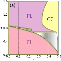
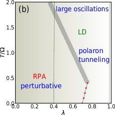
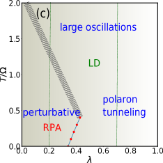
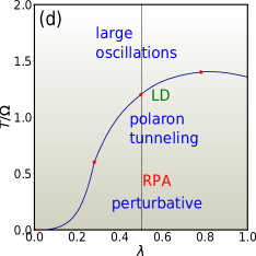
Figure 1: 2D Holstein model: adiabatic ground state and dynamical regimes. (a): Ground state phase diagram obtained via Monte Carlo for $\Omega=0$. We show the undistorted (Fermi liquid - FL), distorted but ‘uncorrelated’ (polaron liquid - PL) and charge correlated (CC) regimes. $n=0.5$ has long range charge order (CO). The $n=0.1,~{}0.4,~{}0.5$ cross sections where we study finite $T$ dynamics are highlighted. (b)-(d): Dynamical regimes of phonon behaviour at $n=0.1,~{}0.4,~{}0.5$ respectively, at $\Omega/t=0.1$. The dimensionless EP coupling is $\lambda=g^{2}/(8Kt)$. The critical coupling $\lambda_{c}$ for transition from the FL to a PL or CO state collapses as $n\rightarrow 0.5$. We observe three broad dynamical regimes - (a) perturbative, (b) polaron tunneling, and (c) large oscillations. In (a), we see small oscillations, $\Delta x\ll x_{pol}$, about homogeneous backgrounds. Regimes (b) and (c) involve ‘large amplitude’ dynamics, where $\Delta x\gtrsim x_{pol}$. A two-branch spectrum emerges in the former.

Figs.1(b)-(d) represent the phonon dynamics at these three densities. The metallic and polaronic regimes at low $T$ are separated by the solid blue lines in the first two panels. The first order discontinuity ends at a temperature $T^{*}\sim 0.5\Omega$.

We have three broad dynamical regimes- (i) perturbative, (ii) polaron tunneling and (iii) large oscillations in each of them. The regions to the bottom left characterize the weak coupling phase. The phonons here belong to regime (i) and are described reasonably well by the RPA approach. There’s a harmonic-anharmonic crossover around $T\sim T^{*}$. Close to $\lambda_{c}$, heating up produces thermally induced polarons, which feature short-range correlations for $n\sim 0.5$. The wavy lines represent the resulting dynamical crossover from (i) to (ii) on the weak coupling side. In the polaronic phase, the low temperature dynamics is that of regime (ii), which crosses over smoothly to (iii) on heating up.

At half-filling, there’s a thermal transition from checkerboard order to a disordered state. The corresponding $T_{CO}$ is sketched in solid blue in Fig.1(d). The low $T$ dynamics is perturbative. Beyond $T\sim 0.5T_{CO}$, correlated tunneling events start showing up appreciably. Beyond $T\sim 1.5T_{CO}$, these events merge with large oscillations.

IV The dilute regime

IV.1 Static properties

The statics is quantified using the distribution of the displacement field $P(x,T)$ and the phonon structure factor $S({\bf q},T)$. The former shows a unimodal to bimodal transition across the critical coupling ($\lambda_{c}=0.8$) at low $T$. Figs.2(a)-(b) (top panel) features the thermal behaviour in the weak ($\lambda/\lambda_{c}=0.5$) and strong ($\lambda/\lambda_{c}=1.2$) coupling regimes. We see $\sim\sqrt{T}$ broadening at weak coupling and gradual smearing of the large distortion peak in the strong coupling case. The weight of the second peak is proportional to electron density. One also observes a quantitative agreement between answers obtained using SPA-MC and LD approaches.

The structure factor $S({\bf q})$ (bottom panel) is benign for all momenta as the polarons don’t influence each other. Therefore, we focus on dynamics in the following section.

    

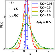
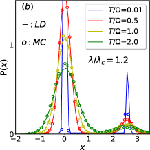
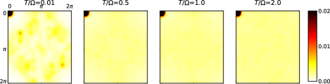
Figure 2: Top: The distribution $P(x)$ of lattice distortions at $n=0.1$ comparing Monte Carlo and Langevin dynamics results. (a) Weak coupling, $\lambda=0.5\lambda_{c}$ (b) Strong coupling, $\lambda=1.2\lambda_{c}$. MC results match with LD at all $T$ and both couplings. Weak coupling shows a sharp unimodal distribution broadening with $T$. $P(x)$ at strong coupling is bimodal, the peak at large $x$ corresponds to polaronic distortions and has weight 0.1 (the electron density). Bottom: Structure factor $S({\bf q},T)$ of distortions at strong coupling. There are no features in ${\bf q}$, except the ${\bf q}=(0,0)$ peak, despite the presence of large distortions.

       

 

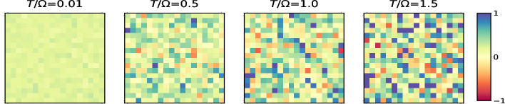
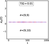
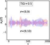
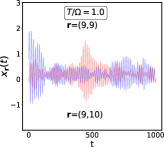
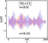
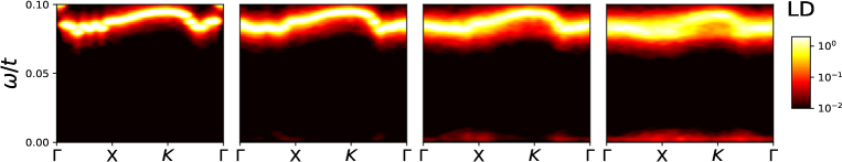
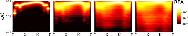
Figure 3: Dilute regime and weak coupling: $n=0.1$ and $\lambda=0.5\lambda_{c}$. Top row: instantaneous configuration $\{x_{i}\}$. Second row: real-time trajectory $x_{i}(t)$ at two sites. Third row: spectral map $|X({\bf q},\omega)|^{2}$ computed using LD. Fourth row: RPA based spectrum for same parameters as in LD. The Brillouin zone trajectory chosen is $(0,0)\rightarrow(\pi,0)\rightarrow(\pi,\pi)\rightarrow(0,0)$. The spatial maps show emergence of weak spontaneous inhomogeneity with increasing $T$. $x_{i}(t)$ shows harmonic fluctuations about a uniform state at low $T$, crossing over to larger amplitude vibrations accompanied by ‘burst’ like events at higher $T$. The later are prominent for $T\sim\Omega$ and generate leading to low frequency weight in $|X({\bf q},\omega)|^{2}$. The RPA spectrum broadens rapidly with increasing $T$, due to the dependence on instantaneous configurations, and also misses the low energy feature.

IV.2 Phonon dynamics

IV.2.1 Weak coupling ($\lambda\ll\lambda_{c}$)

We first discuss the weak coupling ($\lambda/\lambda_{c}=0.5$) regime. The top three rows of Fig.3 are results obtained using Langevin dynamics. First, we plot the snapshots of the displacement field $\{x_{i}\}$. The real-time trajectories for two nearest neighbour sites are featured next, followed by LD based spectra in the third and RPA based spectra in the fourth rows respectively. The first column represents the low temperature regime. Here, the ‘background state’ is translation invariant and the electronic physics is that of a tight-binding model. The phonons execute harmonic oscillations for $T\ll\Omega$ and the resulting dispersion arises out of the bare polarizability $\Pi_{0}({\bf q},\omega)$. The LD and RPA answers match reasonably well. The latter is notionally more accurate as the full frequency dependence of $\Pi_{0}$ is kept.

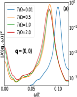
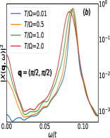
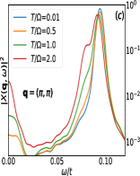
Figure 4: Lineshapes at $n=0.1$ and $\lambda=0.5\lambda_{c}$ and three characteristic momenta- ${\bf q}=(0,0)$, $(\pi/2,\pi/2)$ and $(\pi,\pi)$. Intensities are shown in a log-scale to emphasize the emergence of low energy weight on heating up. The $(0,0)$ mode softens ‘immediately’ compared to the others. Otherwise, the thermal trends are similar for all wavevectors.

       

 

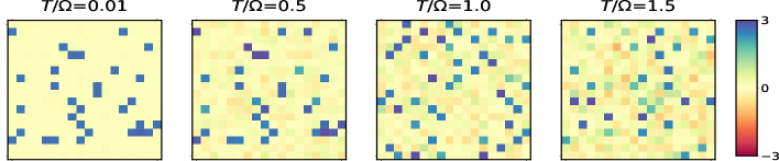
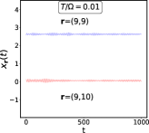
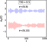
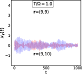
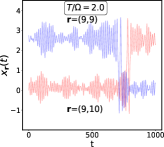
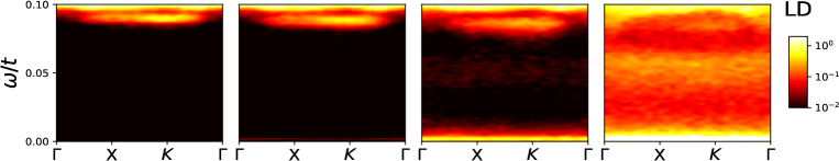
Figure 5: Dilute regime and strong coupling: $n=0.1$ and $\lambda=1.2\lambda_{c}$. Top row: instantaneous configuration $\{x_{i}\}$, showing an essentially uncorrelated patterns of large distortion at all $T$. Second row: real-time trajectory $x_{i}(t)$ at two sites, highlighting their different mean values at low $T$, ‘tunneling’ events (column 3), and large oscillations. Third row: spectral map $|X({\bf q},\omega)|^{2}$ computed using LD. Brillouin zone trajectory as before is $(0,0)\rightarrow(\pi,0)\rightarrow(\pi,\pi)\rightarrow(0,0)$. The first two columns show an almost dispersionless ‘high energy’ feature. The third column shows the emergence of low energy weight due to tunneling events. The highest $T$ shows a broad spectrum due to large amplitude oscillations.

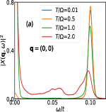
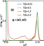
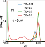
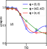
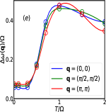
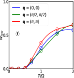
Figure 6: Spectral features at $n=0.1$ and $\lambda=1.2\lambda_{c}$. Top panel: Lineshapes from LD at three momenta- ${\bf q}=(0,0)$, $(\pi/2,\pi/2)$ and $(\pi,\pi)$. The low temperature profile is sharp and unimodal at $(0,0)$, but has a ‘peak splitting’ at the other wavevectors. Thermal behaviour is very similar for all three. The low energy weight transfer is considerable for $T/\Omega\gtrsim 1$. Bottom: Mean frequency, $\bar{\omega}$, linewidth $\Delta\omega({\bf q})$, and low energy weight $w_{low}$ as function of temperature for the three wavevectors. The momentum selectivity is weak.

On heating up to intermediate $T\sim 0.5\Omega$, the amplitudes of oscillations increase and one also sees ‘burst’ like events start to take place. However, at this stage, these are merged with large oscillations. The ‘high energy’ spectra in the LD case remain qualitatively unaltered, but a faint low energy ($\omega\ll\Omega$) weight starts to accumulate. In the third column, we see results for $T\sim\Omega$, by the time the ‘bursts’ become well separated in time and distinct from ‘bare oscillations’. However, spatial correlations are not apparent, as the ‘polaronic distortions’ are created far apart from each other. The spectral signature, within LD, is clearly ‘two-peak’ for most momenta. To emphasize the emergence of low frequency weight, we plot the respective intensities in a logarithmic scale. Finally, at high temperature, the frequency of bursts increase, along with oscillation amplitudes. This strengthens the low energy weight and broadens the high energy band appreciably. We comment that RPA fails to capture the ‘large amplitude’ behaviour of trajectories and consequently gives a gradually broadened spectrum on increasing temperature. This arises from the growing ‘thermal disorder’ of the background states, about which the spectrum of small fluctuations are calculated.

Figs.4(a)-(c) exhibits the thermal dependence of lineshapes at three momentum values- ${\bf q}=(0,0),(\pi/2,\pi/2),(\pi,\pi)$. The basic trends are similar for all three. The softening is accompanied by a low energy weight transfer, which is not significantly momentum selective, as is physically expected.

    

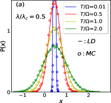
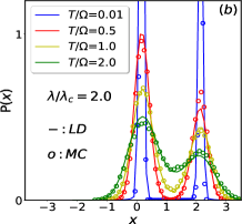
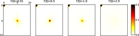
Figure 7: Static indicators at $n=0.4$. Top panels: $P(x)$ at different $T$, comparing MC and LD. (a) - weak coupling, $\lambda/\lambda_{c}=0.5$, (b) - strong coupling, $\lambda/\lambda_{c}=2.0$. Bottom: Structure factor $S({\bf q})$ at strong coupling shows a peak feature at $(\pi,\pi)$ at low $T$, signifying significant charge correlations.

       

 

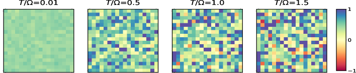
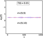
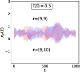
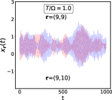
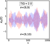
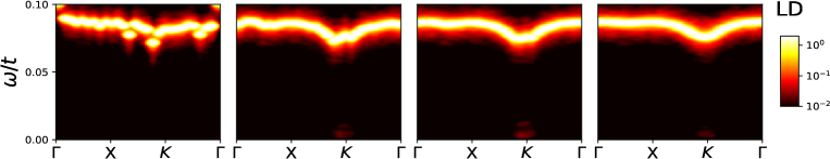
Figure 8: Charge correlated regime and weak coupling: $n=0.4$ and $\lambda=0.5\lambda_{c}$. Top row: instantaneous configuration $\{x_{i}\}$, showing an undistorted $T=0$ configuration evolving into a weakly distorted and short range correlated pattern with increasing $T$. Second row: real-time trajectory $x_{i}(t)$ at two sites, highlighting essentially similar oscillations at neighbouring sites, with an amplitude that grows with $T$. Third row: spectral map $|X({\bf q},\omega)|^{2}$ computed using LD. Brillouin zone trajectory $(0,0)\rightarrow(\pi,0)\rightarrow(\pi,\pi)\rightarrow(0,0)$. The dispersion is essentially $T$ independent with a faint trace of low energy weight that shows up at intermediate $T$ for ${\bf q}\sim(\pi,\pi)$. Overall, in this $n-\lambda$ regime we mainly see a perturbative to large oscillation crossover in the dynamics.

IV.2.2 Strong coupling ($\lambda>\lambda_{c}$)

Fig.5 focusses on the strong coupling regime ($\lambda/\lambda_{c}=1.2$). As before, the top row depicts snapshots of the displacement field. The trajectories on nearest-neighbour sites feature different mean values ($\sim 0$ and $\sim g/K$), signifying that one of them has a trapped electron. Harmonic oscillations are seen in the first column, which grow in amplitude at intermediate $T$ ($\sim 0.5\Omega$). The phonon spectrum is basically composed of the bare band and a split-off weight near ${\bf q}=(\pi,\pi)$. No ‘dispersion’ is discernable, signfying spatially localized phonon modes. The RPA answer agrees well with LD, which means there are no qualitatively new effects brought in by large fluctuations upto this temperature.

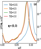
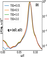
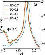
Figure 9: Lineshapes at $n=0.4$ and $\lambda=0.5\lambda_{c}$ and three characteristic momenta- ${\bf q}=(0,0)$, $(\pi/2,\pi/2)$ and $(\pi,\pi)$. Intensities are shown in a log-scale to emphasize the emergence of low energy weight in heating. For this density, the $(\pi,\pi)$ mode shows much more prominent weight transfer at low energies. The high-energy parts have similar thermal behaviour at all ${\bf q}$’s.

However, heating up further ($T\sim\Omega$) dislodges polarons on neighbouring empty spaces. Since this is a dilute system, there’s a lot of room for polarons to move. This creates a prominent, ‘momentum independent’ low-energy band, which is completely missed out by the RPA approach. The physical reason for this weight to crop up is local ‘flip’ moves, which change densities by $0(1)$ on neighbouring sites. We see a reappearance of the polaron for higher $T$ (last column), and a clean occurence of the ‘flip’ amidst large oscillations. The low energy weight is also remarkably increased.

       

 

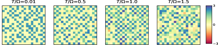
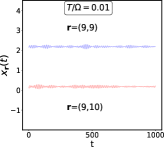
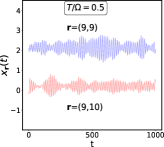
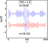
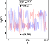
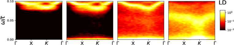
Figure 10: Charge correlated regime, strong coupling: $n=0.4$ and $\lambda=1.2\lambda_{c}$. Top row: Spatial snapshot, 2nd row: real-time trajectories, 3rd row: spectral distribution $|X({\bf q},\omega)|^{2}$ obtained via LD. The BZ trajectory chosen is $(0,0)\rightarrow(\pi,0)\rightarrow(\pi,\pi)\rightarrow(0,0)$. Compared to the dilute case, here the room for polaron tunneling is less. This reduces the probability of ‘dislodging’. At higher $T\gtrsim\Omega$ one observes correlated tunneling moves. The momentum selectivity of low frequency weight transfer is increased on heating.

Figs.6(a)-(c) shows lineshapes at three characteristic momenta, as in the weak coupling case. The lowest $T$ lineshape is bimodal for ${\bf q}=(\pi,\pi)$. Thermal trends are very similar at all momenta. The low energy weight transfer is small till intermediate $T$ ($\sim 0.5\Omega$), but rises dramatically thereafter. The bottom panel focusses on mean ($\bar{\omega}({\bf q})$), width ($\Delta\omega({\bf q})$) and fraction of total spectral weight at low frequency ($w_{low}$) in Figs.6(d)-(f) respectively for the same momentum points. The window for computing $w_{low}$ is chosen to be $0-0.4\Omega$. Again, momentum independence in all these trends are underscored. We see appreciable softening near $T\sim\Omega$ and a sharp rise in dampings beyond $0.5\Omega$.

V The charge correlated regime

V.1 Static properties

The statics again is characterized by $P(x,T)$ and $S({\bf q},T)$. The former is featured for weak and strong coupling regimes in Figs.7(a)-(b) (top panel) and has qualitatively similar features as in the dilute case. The critical coupling $\lambda_{c}=0.4$ at this density. The large distortion peak has more weight compared to the dilute regime.

The structure factor $S({\bf q},T)$ (shown in Fig.7, bottom panel) at low $T$ shows a mild peak at ${\bf q}=(\pi,\pi)$, signifying ‘charge order’. We comment that this is an artifact of neglecting quantum fluctuations However, above a charge correlation scale $T_{CC}\sim\Omega$, this peak is significantly subdued and the system becomes thermally disordered.

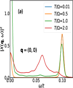
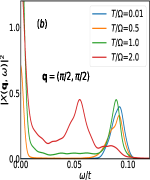
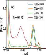
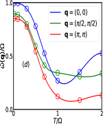
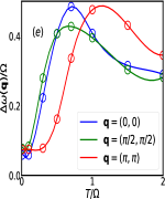
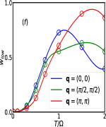
Figure 11: Spectral features at $n=0.4$ and $\lambda=1.2\lambda_{c}$. Top: Lineshapes obtained using LD for three momenta- ${\bf q}=(0,0)$, $(\pi/2,\pi/2)$ and $(\pi,\pi)$. The low $T$ result has a ‘peak splitting’ at $(\pi,\pi)$. Thermal behaviour is clearly momentum selective. Bottom: Mean frequency, $\bar{\omega}$, linewidth, $\Delta\omega({\bf q})$, and low energy weight, $w_{low}$ for the same three wavevectors. The $(\pi,\pi)$ mode shows enhanced softening. Low-energy weight rises similarly for all ${\bf q}$’s.

V.2 Phonon dynamics

V.2.1 Weak coupling ($\lambda\ll\lambda_{c}$)

Fig.8 summarizes our findings on the full phonon spectrum in the weak coupling ($\lambda/\lambda_{c}=0.5$) scenario. The top row features real space snapshots, followed by real-time trajectories in the second row. The overall behaviour is similar to the dilute case, with the main difference being a correlation between nearest neighbours in the ‘burst’ like events. The impact of this is directly seen as a faint low-frequency weight at ${\bf q}=(\pi,\pi)$, visible from $T\sim 0.5\Omega$. The high-energy band is much more coherent within the LD approach compared to RPA. This happens as the former captures crucial anharmonic fluctuations, while the latter is limited to gaussian fluctuations on ‘thermally disordered’ backgrounds. Once again, we’ve used a log-scale to emphasize the low frequency weights. We also comment that the momentum selective small weight transfer gets quantitatively more prominent on moving closer to the crossover ($\lambda\sim\lambda_{c}$).

In Figs.9(a)-(c), the detailed lineshapes in this regime reveal that the low energy weight transfer is most prominent at ${\bf q}=(\pi,\pi)$, the wavevector relevant for short-range correlations. The high energy thermal trends are similar for all momenta. However, the $(0,0)$ mode softens considerably on mild heating, closely followed by the $(\pi,\pi)$ mode.

V.2.2 Strong coupling ($\lambda>\lambda_{c}$)

Fig.10 highlights the strong coupling ($\lambda/\lambda_{c}=2.0$) dynamics in the high density regime. The snapshots clearly depict a dense polaronic system at low temperature. The nearest neighbour trajectories reveal the usual harmonic-anharmonic crossover in the first two columns. However, rare ‘flip’ moves are present even for $T\sim 0.5\Omega$, generating some low-frequency weight quantified in detail later. Moving close to the bare phonon scale ($T\sim\Omega$), interesting ‘stray’ flips are seen, which accentuate the low-frequency weight transfer. The high energy band retains its low $T$ shape. At even higher temperatures, this band itself moves to lower frequencies. The spatial correlations amongst flip moves strengthen, leading to increased momentum selectivity. On further heating, the correlations weaken. The RPA method, as before, gives progressive dampings on heating and fails to capture the rich thermal behaviour.

Fig.11 summarizes the detailed phonon properties. First, in 11(a)-(c), the lineshapes (top panel) at three characteristic wavevectors $(0,0)$, $(\pi/2,\pi/2)$ and $(\pi,\pi)$ reveal that there’s indeed more pronounced momentum selectivity compared to the dilute case. The low temperature lineshapes are unimodal for the first two while the $(\pi,\pi)$ mode features a bifurcation. On heating up, even at intermediate $T\sim 0.5\Omega$, there’s a $\sim 20\%$ weight transfer near zero frequency. This is related to rare thermal tunneling moves. The bottom panel (Figs.11(d)-(f)) shows prominent softening at $(\pi,\pi)$ compared to other momenta, although broadenings show an opposite trend. Low energy weight rises similarly for all wavevectors.

VI Commensurate filling and charge order

In this section, we summarize the phonon properties for charge ordered ($n=0.5$) systems. In this case, $\lambda_{c}=0$. The system has an order-disorder thermal transition at $T\sim 2\Omega$ for $\lambda=0.5$, that falls as $\sim 1/\lambda$ at strong coupling.

VI.1 Static properties

The top row of Fig.12 shows the $P(x)$ distributions (a) and structure factor $S(\pi,\pi)$ (b) at this density for various temperatures. The results obtained using Langevin dynamics and Monte Carlo agree very well over all thermal regimes. The order-disorder transition at this coupling takes place around $T\sim 0.1t$. The distribution of distortions is bimodal and symmetric about $x=1.0$ at low $T$. Thermal effects broaden the peaks and almost merge them for $T\sim 2T_{c}$.

VI.2 Phonon dynamics

The bottom two rows of Fig.12 feature spectral maps for $n=0.5$. The top panel shows spectra obtained using the LD approach while the bottom one exhibits RPA based spectra. We see that the perturbative theory fails to capture the low-energy weight transfer at $(\pi,\pi)$ near $T\sim\Omega\sim T_{c}$. These are evidently due to non-Gaussian ‘correlated flip’ moves in the lattice. The high temperature dynamics is that of a ‘disordered polaron liquid’, also captured by the LD approach and not by the RPA, which just gives a very broad spectrum.

    

    

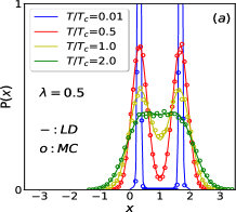
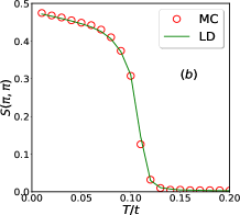
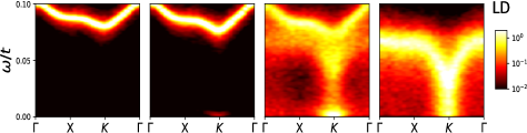
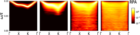
Figure 12: Features at $n=0.5$, increasing $T$ on a CO state. Top row: (a) Distribution of distortions, $P(x)$, and (b) structure factor $S(\pi,\pi)$. The former shows symmetric bimodal profile at all temperatures. The structure factor is shown only for the ordering wavevector, and shows an order-disorder transition for $T_{c}\sim 0.1t$. Bottom: Phonon spectra computed using LD (upper row) and RPA (lower row). The dramatic low-energy weight transfer near criticality is captured by the former, while RPA just shows an increasingly broad spectrum due to the disordered thermal backgrounds. Beyond $T_{c}$, LD reveals dynamics in the thermal ‘polaron liquid’.

VII Discussion

VII.1 RPA versus the Langevin approach

We’ve used two complementary strategies to investigate the phonon physics in the Holstein model, namely traditional RPA and Langevin dynamics. Both of them are viable in the physically relevant adiabatic regime, where phonon variables are slow. The former is restricted to small amplitude quantum fluctuations about finite temperature static ‘backgrounds’, while the latter can access large amplitude classical dynamical fluctuations.

In the strong coupling scenario, large distortions are already ‘preformed’ in the lattice. Within RPA, we only probe small amplitude fluctuations about the ‘thermally disordered’ backgrounds. These don’t faithfully represent the true dynamics of the system, which involves re-organization of the polarons on neighbouring sites. These are rare, non-Gaussian moves. The Langevin dynamics method approximately captures these events and hence gets interesting low-energy signatures, which RPA fails to access. In other words, while the latter approach does contain large distortions at the static level, their dynamics ‘as a whole’ is missed out. One only calculates the impact of small excursions on top of the ‘distorted’ states. Fig.13 illustrates the difference in the family of fluctuations accessed by the respective methods.

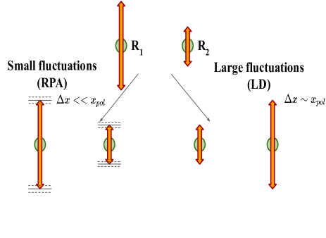
Figure 13: Schematic cartoons of the RPA and LD schemes. In the former, one explores small amplitude fluctuations about ‘large’ or ‘small’ background distortions. Within LD, the novelty is to capture ‘swapping’ moves of large and small distortions on adjacent sites.

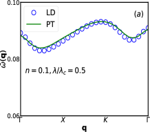
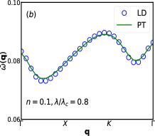
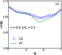
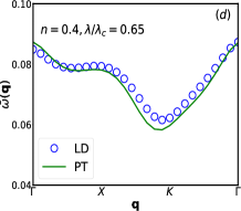
Figure 14: Phonon dispersions ($\bar{\omega}({\bf q})$) obtained using Langevin dynamics (LD) and standard perturbation theory (PT), implemented in momentum space, in the weak coupling scenario. We show four typical parameter points. The top row features results in the dilute regime, while the bottom depicts the correlated case. We observe a quantitative agreement between the low $T$ LD answer and the perturbative one in all cases.

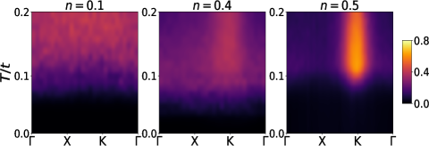
Figure 15: Maps of low energy weight fraction ($w_{low}$) in the (${\bf q},T$) plane for three typical densities- $n=0.1$ (dilute) , $n=0.4$ (correlated) and $n=0.5$ (ordered). The x-axis denotes the typical ${\bf q}$ trajectory ($\Gamma-X-K-\Gamma$) and the y-axis is temperature $T/t$. The parameter points chosen are- $\lambda/\lambda_{c}=1.2$ for $n=0.1$, $\lambda/\lambda_{c}=2.0$ for $n=0.4$, and $\lambda=0.5$ for $n=0.5$. The crucial feature is the growing momentum selectivity on moving to higher densities. One also observes an early onset of increase in $w_{low}$ with respect to $T$ in the correlated case compared to the dilute and ordered ones.

We comment that similar effects are crucial in other electron correlation models, like Hubbard, in the strong coupling scenario. In the auxiliary field language, the ‘moments’ at strong coupling have a reasonably fixed amplitude. But, large angular fluctuations dictate the dynamics, instead of ‘small amplitude’ oscillations as captured within RPA. Hence, the latter method again fails to describe finite temperature collective mode spectrum.

While it’s true that over a wide $T$ window, Langevin approach is better, the present equation is derived using several drastic approximations, notably ‘Ohmic dissipation’ and ‘thermal noise’. As a consequence, we relegate the phonon variables to the classical level, which freeze at zero temperature. A more complex, self-consistent noise and damping could alleviate the issue in principle and make the method accurate even at low $T$.

VII.2 Low temperature dispersion and perturbation theory

We compared the phonon dispersions obtained at low $T$ using the LD method with a standard perturbative calculation done in $({\bf q},\omega)$ space in the weak coupling regime. The results, shown in Figs.14(a)-(d), show a quantitative agreement. The match is better in the dilute ($n=0.1$) case compared to the correlated ($n=0.4$) one. We comment that the LD answer contains the effect of static bare polarizability $\Pi_{0}({\bf q})$, and not the full frequency dependent $\Pi_{0}({\bf q},\omega)$, as in the RPA. However, at weak coupling, this distinction is irrelevant.

VII.3 Anharmonic theory and phonon damping

Beyond the quadratic phonon theory, one may add cubic non-linearities to obtain interaction induced phonon damping. This is already discussed in our previous paper sauri , where it’s shown that the linear behaviour of phonon linewidth ($\Gamma({\bf q})$) can be explained using a perturbative approach. The argument doesn’t depend on the electron density or nature of the background state and hence goes through also in the present case.

VII.4 Low-energy weight in the polaronic phase

The highlight of the Langevin dynamics method in the strong coupling phase is the capturing of ‘thermal tunneling’ moves. These events are rare at low $T$, but become progressively frequent at intermediate to high temperatures and are crucial in restoring the ‘translational symmetry breaking’ observed within the adiabatic limit. The spectral signature, as shown in detail earlier, is the accumulation of low frequency ($\omega\ll\Omega$) weight. We choose a cutoff of $0.4\Omega$ and integrate the obtained spectral weight upto this, subsequently normalizing by the total weight. As shown in Fig.15, this low energy weight fraction ($w_{low}$) becomes increasingly momentum selective as one approaches commensurate filling. Moreover, one observes (i) quantitatively larger values in the dilute case compared to the correlated one beyond a threshold ($T\sim\Omega$), related to more room for tunneling, and (ii) a comparatively earlier onset of increase with respect to $T$ in the correlated case. The half-filling scenario exhibits a pronounced temperature sensitivity, owing to critical ‘domain oscillations’.

VIII Conclusion

We have studied the phonon dynamics in the two dimensional Holstein model across the polaronic crossover in three different density regimes: dilute, charge correlated, and charge ordered. We explored two different approaches- (i) a generalisation of the traditional RPA to finite temperature, and (ii) a Langevin dynamics strategy employing a force derived from the electronic Hamiltonian. Both methods reproduce the standard perturbative phonons at weak coupling. Approaching the polaronic transition from this end, the RPA strategy becomes progressively inaccurate and mainly yields a large damping due to the background thermal disorder. The Langevin approach, however, gives more coherent phonons as it takes anharmonic effects into account correctly. In the polaronic phase the Langevin approach captures the slow polaron tunneling events and the corresponding low energy spectral weight, an effect completely missed by the RPA due to its perturbative ‘low amplitude’ character. We have quantified these trends for varying coupling and temperature. Our method can handle real lattice geometries, strong coupling, finite temperature, and collective effects at finite electron density, with modest computational effort. This paper sets the framework based on which we will discuss inelastic neutron results in specific materials in the near future.

Acknowledgement: We acknowledge the use of HPC clusters at HRI. SB acknowledges fruitful discussions with Arijit Dutta and Abhishek Joshi. The research of SB was partly supported by an Infosys scholarship for senior students. The research of SP was partly supported by the Olle Engkvist Byggmästare Foundation.

IX Appendix

In terms of the fermion eigenvalues and eigenvectors on a given $x_{i0}$ background, we may write down the full polarization $\Pi_{ij}(\omega)$ as-

$$\Pi_{ij}(\omega)=-\sum_{m}\sum_{n}u_{im}u_{jm}u_{in}u_{jn}\frac{n_{F}(\epsilon_{m})-n_{F}(\epsilon_{n})}{\omega+i\eta-(\epsilon_{m}-\epsilon_{n})}$$ (33)

where the $u$’s are site amplitudes of eigenfunctions for a given configuration, $\epsilon$’s being the eigenvalues. $n_{F}$’s are Fermi distribution functions.

This reduces (in the static polarization approximation) to

$$\Pi^{0}_{ij}=\sum_{m}\sum_{n}u_{im}u_{jm}u_{in}u_{jn}\frac{n_{F}(\epsilon_{m})-n_{F}(\epsilon_{n})}{(\epsilon_{m}-\epsilon_{n})}$$ (34)

for $m\neq n$ and

$$\Pi^{0}_{ij}=-\beta\sum_{m}(u_{im}u_{jm})^{2}n_{F}(\epsilon_{m})(1-n_{F}(\epsilon_{m}))$$ (35)

for $m=n$.

To find the phonon propagator from the full $\Pi_{ij}(\omega)$, one has to solve the Dyson’s equation

$$D^{-1}_{ij}(\omega)=D^{-1}_{0,ij}(\omega)+g^{2}\Pi_{ij}(\omega)$$ (36)

In the approximated theory, one may do a real space diagonalization of the matrix-

$$M_{ij}=K\delta_{ij}+{g}^{2}\Pi_{ij}$$ (37)

to get the phonon eigenmodes. The eigenvalues give us the renormalized stiffness constants. Finally, in terms of these and the new eigenvectors, the phonon propagator reads-

$$D_{ij}=\sum_{m}V_{im}{V_{jm}}\left(\frac{1}{\omega+i\eta-\xi_{m}}-\frac{1}{\omega-i\eta+\xi_{m}}\right)$$ (38)

where $\xi_{m}$’s are phonon frequencies obtained from the stiffnesses and $V$’s denote site amplitudes of the bosonic eigenfunctions. $\eta$ is a positive infinitesimal, as usual.

References

- [1] A.S. Alexandrov, Polarons in Advanced Materials, Springer (2007).
- [2] L. Degiorgi, E.J. Nicol, O.Klein, G.Gruner, P.Wachter, S.M. Huang, J.Wiley, and R.B. Kaner, Phys. Rev. B 49, 10 (1994).
- [3] A.V. Puchkov, T.Timusk, M.A. Karlow, S.L.Cooper, P.D. Han, and D.A. Payne, Phys. Rev. B 54, 6686 (1996).
- [4] Y. Okimoto and Y. Tokura, J.Supercond. 13, 271 (2000).
- [5] Y. Tokura, Colossal Magnetoresistive Oxides, CRC Press (2000).
- [6] H. A. Mook, B.C. Chakoumakos, N.Mostoller, A.T. Boothroyd, and D.McK. Paul, Phys. Rev. Lett. 69, 2272 (1992).
- [7] R.J. McQueeney, Y. Petrov, T. Egami, M. Yethiraj, G. Shirane, and Y. Endoh, Phys. Rev. Lett. 82, 628 (1999).
- [8] F. Weber, N. Aliouane, H. Zheng, J.F. Mitchell, D.N. Argyriou, and D.Reznik, Nature Materials 8, 798 (2009).
- [9] F. Weber, S. Rosenkranz, J.-P. Castellan, R. Osborn, H. Zheng, J.F. Mitchell, Y. Chen, Songxue Chi, J. W. Lynn, and D. Reznik, Phys. Rev. Lett. 107, 207202 (2011).
- [10] M. Maschek, D. Lamago, J.-P. Castellan, A. Bosak, D. Reznik, and F. Weber, Phys. Rev. B 93, 045112 (2016).
- [11] M. Maschek, J.-P. Castellan, D. Lamago, D. Reznik, and F. Weber, Phys. Rev. B 97, 245139 (2018).
- [12] R. Kajimoto, M. Fujita, K. Nakajima, K. Ikeuchi, Y. Inamura, M. Nakamura and T. Imasoto, Journal of Physics, Conference Series 502 012056 (2014).
- [13] D. Reznik Advances in Condensed Matter Physics, Vol. 2010, Article ID 523549 (2010).
- [14] H. Miao, D. Ishikawa, R.Heid, M. Le Tacon, G. Fabbris, D. Meyers, G.D. Gu, A.Q.R. Baron and M.P.M. Dean, arXiv 1712.04554.
- [15] M. Braden, W. Reichardt, S. Shiryaev and S.N. Barilo, Physica C 378-381 (2002) 89-96.
- [16] J. Bonca, S.A. Trugman, and I. Batistic, Phys. Rev. B 60, 1633 (1999).
- [17] A.S. Alexandrov, V.V. Kabanov, and D.K. Ray, Phys. Rev. B 49, 9915 (1994).
- [18] H. Fehske, J. Loos, and G. Wellein, Z. Phys. B 104, 619 (1997).
- [19] A.B. Krebs and S.G. Rubin, Phys. Rev. B 49, 11808 (1994).
- [20] Glen L. Goodvin, Mona Berciu and George A. Sawatzky, Phys. Rev. B 74, 245104 (2006).
- [21] Patrizia Benedetti and Roland Zeyher, Phys. Rev. B 58, 14320 (1998).
- [22] A. Deppeler and A.J. Millis, Phys. Rev. B 65, 100301(R) (2002).
- [23] Stefan Blawid, Andreas Deppeler, and A.J. Millis, Phys. Rev. B 67, 165105 (2003).
- [24] S. Ciuchi, F. de Pasquale, S. Fratini and D. Feinberg, Phys. Rev. B 56, 4494 (1997).
- [25] M. Capone and S. Ciuchi, Phys. Rev. Lett. 91, 186405 (2003).
- [26] B. Poornachandra Sekhar, Sanjeev Kumar and Pinaki Majumdar, Europhys. Lett. 68, 564 (2004).
- [27] A.B. Migdal, Sov. Phys. JETP 7, 996, (1958); G.M. Eliashberg, ibid. 11 696 (1960).
- [28] R. Blankenbecler, D.J. Scalapino, and R.L. Sugar, Phys. Rev. D 24, 8 (1981).
- [29] A. Georges, G. Kotliar, W. Krauth, and M.J. Rozenberg, Rev. Mod. Phys. 68, 13 (1996).
- [30] C.E. Creffield, G. Sangiovanni, and M. Capone, Eur. Phys. J. B 44, 175 (2005).
- [31] M Hohenadler, H Fehske, and F F Assaad, Phys. Rev. B 83, 115105 (2011).
- [32] D. Meyer, A.C. Hewson, and R. Bulla, Phys. Rev. Lett. 89, 196401 (2002).
- [33] J. Loos, M. Hohenadler, A. Alvermann and H. Fehske, J. Phys.: Condens. Matter 18 (2006) 7299-7312.
- [34] J. P. Hague, J. Phys..:Condens. Matter 15 (2003) 2535-2550.
- [35] N.C. Costa, T. Blommel, W.-T. Chiu, G. Batrouni and R.T. Scalletar, Phys. Rev. Lett. 120, 187003 (2018).
- [36] Gia-Wei Chern, Kipton Barros, Zhentao Wang, Hidemaro Suwa, and Cristian D. Batista, Phys. Rev. B 97, 035120 (2018).
- [37] S. Bhattacharyya, S. S. Bakshi, S. Kadge, and P. Majumdar, Phys. Rev. B 99, 165150 (2019).
- [38] Sanjeev Kumar and Pinaki Majumdar, arXiv:cond-mat/0406082 (2004).
- [39] D. Mozyrsky, M.B. Hastings, and I. Martin, Phys. Rev. B 73, 035104 (2006).
- [40] P. E. Kloeden and E. Platen, Numerical Solution of Stochastic Differential Equations, Springer, Berlin (1992).