H₂ emission from non-stationary magnetized bow shocks

Abstract

When a fast moving star or a protostellar jet hits an interstellar cloud, the surrounding gas gets heated and illuminated: a bow shock is born which delineates the wake of the impact. In such a process, the new molecules that are formed and excited in the gas phase become accessible to observations. In this article, we revisit models of H₂ emission in these bow shocks. We approximate the bow shock by a statistical distribution of planar shocks computed with a magnetized shock model. We improve on previous works by considering arbitrary bow shapes, a finite irradiation field, and by including the age effect of non-stationary C-type shocks on the excitation diagram and line profiles of H₂. We also examine the dependence of the line profiles on the shock velocity and on the viewing angle: we suggest that spectrally resolved observations may greatly help to probe the dynamics inside the bow shock. For reasonable bow shapes, our analysis shows that low velocity shocks largely contribute to H₂ excitation diagram. This can result in an observational bias towards low velocities when planar shocks are used to interpret H₂ emission from an unresolved bow. We also report a large magnetization bias when the velocity of the planar model is set independently. Our 3D models reproduce excitation diagrams in BHR71 and Orion bow shocks better than previous 1D models. Our 3D model is also able to reproduce the shape and width of the broad H₂ 1-0S(1) line profile in an Orion bow shock.

1 Introduction

Jets or winds are generated in the early stages and the late phases of stellar evolution. The impact of high velocity flows on the interstellar medium (ISM) creates a shock. When the star moves with respect to the surrounding gas, or when the tip of a jet penetrates the ISM, the shock working surface assumes a curved shape called ’bow shock’.

The angle between the impinging gas velocity and the normal to the shape can vary along this bow. It also affects the angle of the ambient magnetic field. As a result, the local effective entrance velocity and the transverse magnetic field change along the shock working surface. This leads to differences in the local physical and chemical conditions, which cause varying emission properties throughout the bow shock.

As a result, the global emission spectrum of a bow shock is expected to differ from that of a 1D plane parallel shock. Accurate modeling of the emission properties of bow shocks is thus an important goal if we wish to retrieve essential properties of the system from observations, such as the propagation speed, the age, the environment density and the magnetic field. Molecular hydgrogen is a particularly important tracer, as it dominates the shock cooling up to the dissociation limit (if the pre shock medium is molecular), and it emits numerous lines from a wide range of upper energy levels within a single spectrometer setting (in the K-band for ro-vibrational $\Delta v=1$ lines; in the mid-IR range $8-28\mu$m for the first pure rotational lines). In principle, the H₂ emission originating from bow shocks can be predicted by performing 2D or 3D numerical simulations, but the latter have been so far limited to single-fluid "jump" shocks, J-type (e.g. Raga et al. 2002; Suttner et al. 1997). Up to now they cannot treat "continuous" C-type shocks, where ion-neutral decoupling occurs in a magnetic precursor (Draine & McKee 1993). Such situation is encountered in the bow shock whenever the entrance speed drops below the magnetosonic speed in the charged fluid. To address this case, a second approach to predict H₂ emission from bow shocks is to prescribe a bow shape and treat each surface element as an independent 1D plane-parallel J-type or C-type shock, assuming that the emission zone remains small with respect to the local curvature. This approach was first introduced by Smith & Brand (1990a) and Smith et al. (1991a) using simplified equations for the 1D shock structure and cooling. The validity of this approach was recently investigated by Kristensen et al. (2008) and Gustafsson et al. (2010) using refined 1D steady-state shock models that solve the full set of magneto-hydrodynamical equations with non-equilibrium chemistry, ionisation, and cooling.

Kristensen et al. (2008) studied high angular resolution H₂ images of a bow shock in the Orion BN-KL outflow region, performing several 1D cuts orthogonal to the bow trace in the plane of the sky. They fitted each cut separately with 1D steady shock models proposed by Flower & Pineau des Forêts (2003). They found that the resolved width required C-shocks, and that the variation of the fitted shock velocity and transverse magnetic field along the bow surface was consistent with a steady bow shock propagating into a uniform medium. This result provided some validation for the ’local 1D-shock approximation’ when modeling H₂ emission in bow shocks, at least in this parameter regime. Following this idea, Gustafsson et al. (2010) built 3D stationary models of bow shocks by stitching together 1D shock models. They then projected their models to produce maps of the H₂ emission in several lines which they compared directly to observations. They obtained better results than Kristensen et al. (2008) thanks to the ability of the 3D model to account both for the inclination of the shock surface, with respect to the line of sight, and the multiple shocks included in the depth of their 1D cuts. The width of the emission maps was better reproduced.

In this article, we extend Gustafsson et al. (2010)’s works on H₂ emission by computing the excitation diagram and line profiles integrated over the bow, and by considering the effect of short ages where C-shocks have not yet reached steady-state. Our method also increases the scope of Gustafsson et al. (2010) to arbitrary bow shapes (we do not restrict the bow shape profile to power laws). Using time-dependent simulations, Chièze et al. (1998) discovered that young C-type shocks, the age of which is smaller than the ion crossing time, are composed of a magnetic precursor and a relaxation layer separated by an adiabatic J-type front. Lesaffre et al. (2004b) later showed that the magnetic precursor and the relaxation layer were truncated stationary models of C-type and J-type shocks, respectively. In the present work, we make use of these CJ-type shocks to explore the age dependence of the H₂ emission. Non-steady shocks are more likely to occur in low density media, where the time-scales are generally longer than those driving the mechanisms of these shocks: hence, we consider lower densities than Gustafsson et al. (2010), down to 100 cm^-3. As in Lesaffre et al. (2013), we include the grain component as part of the charged fluid, which singificantly lowers the magnetosonic speed. In addition the Paris-Durham code (Flower et al. 2003; Flower & Pineau des Forêts 2015), recently improved by Lesaffre et al. (2013), now allows to consider finite UV irradiation conditions and we use a standard interstellar irradiation field of $G_{0}$=1 (Draine 1978) throughout the paper. This lowers slighlty further the magnetosonic speed as the ionisation degree/fraction increases but we checked it does not introduce critical changes for the H₂ emission properties. The lower magnetosonic speed above which no C-shock propagates and the truncated precursor in young CJ-type shocks both act in a way so that they give more weight to J-type shocks compared to Gustafsson et al. (2010), who had their J-type shocks H₂ emission dimmed by dissociation above $\simeq$15-20 km s^-1 due to the larger densities. Finally, we also investigate the line profiles which were not examined by Gustafsson et al. (2010).

We study how the geometry influences the distribution of shock entrance velocity and transverse magnetic field in section 2. We present our grid of planar shock models at finite ages in section 3. In the next section 4, we combine the planar shock models to build 3D models of bow shocks. We examine the observable H₂ excitation diagram and the potential biases which arise when 1D models are fit to intrinsically 3D models. We apply our 3D model to constrain parameters of the BHR71 bipolar outflow and for a bow shock in Orion. Finally, We study the properties of H₂ line profiles and show how it can be used to retrieve dynamical information. We summarise and conclude in section 5.

2 The model

As in Gustafsson et al. (2010), we assume that the 3D bow shock is made of independent planar shocks. In fact, we neglect the curvature effects and the friction between different 1D shock layers, the gradients of entrance conditions in the planar shock models, and the possible geometrical dilatation in the post-shock: our approximation is valid as long as the curvature radius of the bow shock is large with respect to the emitting thickness of the working surface.

2.1 Geometry and coordinate system

We consider an axisymmetric 3D bow shock around a supersonic star (or a jet) travelling at the speed of $-\textbf{u}_{0}$ relative to an ambient molecular cloud assumed to be at rest. In the frame of the star, the impinging velocity is therefore uniform and equal to $\textbf{u}_{0}$. The apex of the bow shock is at position A and the star (or a reference point in the jet) at position O (figure 1). The axis of symmetry chosen as the z-axis is therefore along the direction (AO). The observer is assumed to lie in the (Oxz) plane and the y-direction is chosen such that (Oxyz) is direct. The axisymmetric shape of the bow shock is completely determined by the function $x=f(z)$. The local position along the planar shock can be specified by the angle between the incoming flow and the tangent to the surface $\alpha=\arccos(u_{\bot}/u_{0})$ (see Smith & Brand, 1990a, figure 1), and by the angle $\varphi$ between the radius and the x-axis in the (xy) plane of projection.

The impinging velocity can be expressed as $\textbf{u}_{0}=\hat{\textbf{t}}u_{\parallel}+\hat{\textbf{n}}u_{\bot}=u_{0}(\hat{\textbf{t}}\cos\alpha+\hat{\textbf{n}}\sin\alpha)$, where $\hat{\textbf{n}}(-\cos\alpha\cos\varphi,-\cos\alpha\sin\varphi,\sin\alpha)$ is the unit normal vector pointing inside the bow and $\hat{\textbf{t}}(\sin\alpha\cos\varphi,\sin\alpha\sin\varphi,\cos\alpha)$ is the unit tangent vector along the working surface. The effective shock speed at the local point is $v_{s}=u_{\bot}=u_{0}\sin\alpha$. Away from the axis of symmetry, the effective entrance velocity into the shock decreases down to the sound speed $c_{s}$ in the ambient medium. Beyond this point, the shock working surface is a cone of opening angle $\alpha_{0}=\arcsin(c_{s}/u_{0})$, wider as the terminal velocity is closer to the sound speed. In this paper, we mainly focus on the “nose” of the bow shock where $u_{\bot}>c_{s}$, and we neglect the emission from these conical “wings”, or we simply assume that they fall outside the observing beam.

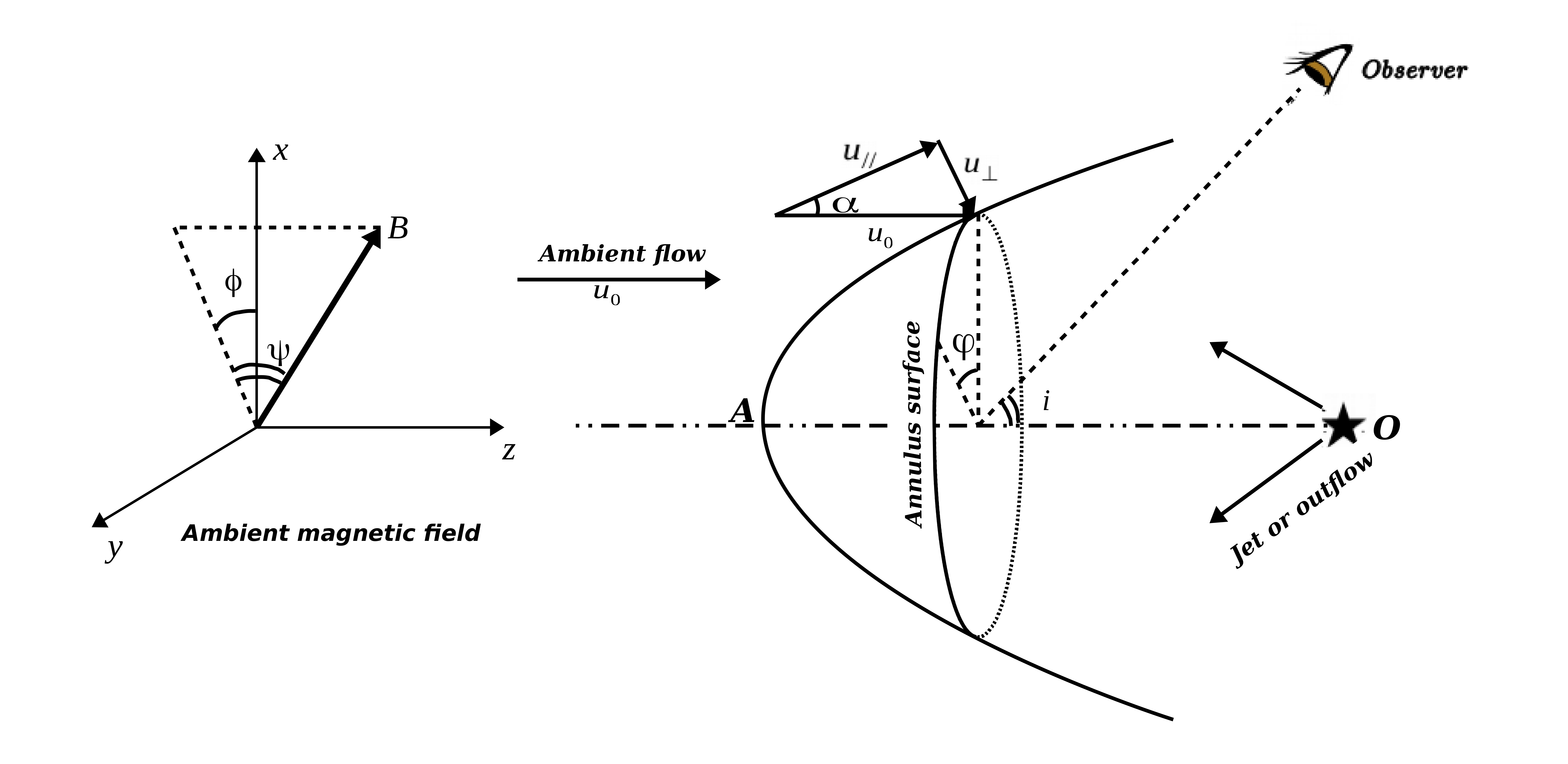
Figure 1: Morphology of a magnetized bow shock in the frame of a star or a jet. The direction of the magnetic field is expressed by the angles $\psi$ and $\phi$. The observer lies at an angle $i$ to the z-axis in the Oxz plane.

The orientation of the line-of-sight of the observer in the $(x,z)$ plane is defined by the inclination angle $i$: $\hat{\textbf{l}}(\sin i,0,\cos i)$. The ambient uniform magnetic field is identified by the obliqueness $\psi$ and the rotation $\phi$: $\textbf{B}/B_{0}=(\cos\psi\cos\phi,\cos\psi\sin\phi,\sin\psi)$. For each bow shock, $\psi$ and $\phi$ are fixed.

2.2 Distribution function of the local planar shock velocity

This section aims at computing the fraction $P(u_{\bot})\mathrm{d}u_{\bot}$ of planar shocks with an entrance planar shock $u_{\bot}$ within $\mathrm{d}u_{\bot}$ in a given bow shock shape. This will help us building a model for the full bow shock from a grid of planar shocks.

Considering the shock geometry as prescribed in section 2.1, we aim at obtaining the formula for the unit area $ds$ corresponding to these shocks as a function of $du_{\bot}$.

The norm of a segment $dl$ on the $(x,z)$ section of the bow shock surface is:

$$dl=\sqrt{dx^{2}+dz^{2}}=\sqrt{1+f^{\prime 2}(x)}dx.$$ (1)

Now, we take that segment and rotate it around the $z$-axis, over a circle of radius $x$. The area ($ds$) of the bow shock’s surface swept by this segment can be expressed as:

$$ds=2\pi xdl=2\pi x\sqrt{1+f^{\prime 2}(x)}dx\mbox{.}$$ (2)

Note that the angle $\alpha$ defined in figure 1 is also the angle between the segment $dl$ and the differential length $dz$ along the $z$-axis. Then, the tangent of the angle $\alpha$ can be set as

$$\tan\alpha=\frac{dx}{dz}=\frac{1}{f^{\prime}(x)}\mbox{.}$$ (3)

In all generality, the relationship between $\alpha$ and $u_{\bot}$ will be realized according to whether we consider the shock in the ambient medium or in the stellar wind or jet. Then, $ds$ as a function of $du_{\bot}$ can be obtained by replacing that relation into equation 2. However, we will only focus here on the bow shock in the ambient material. In that case, the norm of the effective velocity (i.e., the effective normal velocity $u_{\bot}$) is related to the norm of the incident velocity $\textbf{u}_{0}$ through the angle $\alpha$ as

$$u_{\bot}=u_{0}\sin\alpha\rightarrow\alpha=\arcsin(\frac{u_{\bot}}{u_{0}})\mbox{.}$$ (4)

Now, $x$ can be expressed as a function of $u_{\bot}$ by substituting equation 4 into equation 3:

$$\tan[\arcsin(\frac{u_{\bot}}{u_{0}})]=\frac{1}{f^{\prime}(x)}\rightarrow x=f^{\prime-1}\{\cot[\arcsin(\frac{u_{\bot}}{u_{0}})]\}=g(u_{\bot})\mbox{.}$$ (5)

In equation 2, the unit are $ds$ of the shock is a function of the coordinate $x$, while in equation 5, the coordinate $x$ is a function of the effective shock velocity $u_{\bot}$. To sum up, we can obtain $ds$ as a function of $u_{\bot}$:

$$\begin{split}ds(u_{\bot})&=2\pi g(u_{\bot})\sqrt{1+\cot^{2}[\arcsin(\frac{u_{\bot}}{u_{0}})]}g^{\prime}(u_{\bot})du_{\bot}\\ &=\pi\sqrt{1+\cot^{2}[\arcsin(\frac{u_{\bot}}{u_{0}})]}\ d[g^{2}(u_{\bot})]\end{split}$$ (6)

Finally, the distribution function of shock velocities is simply defined as

$$P(u_{\bot})=\frac{ds(u_{\bot})}{\int_{c_{s}}^{u_{0}}ds},$$ (7)

so that the integral of $P(u_{\bot})$ is normalized to unity. Note that the lower limit of the integral is the sound speed in the ambient medium. This implicitly assumes that we only focus on the “nose” of the bow shock, where $u_{\bot}<c_{s}$. One could include the conical “wings” by adding a Dirac distribution $\delta(u_{\bot}=c_{s})$. Conversely, one could also narrow down the integration domain if the beam intersects a smaller fraction of the bow. We implemented this mathematical formulation numerically to compute the distribution $P$ from an arbitrary input function $f$. We obtained results that agree with those obtained using the analytical expressions when the shape assumes a power-law dependence $z\sim x^{\beta}$.

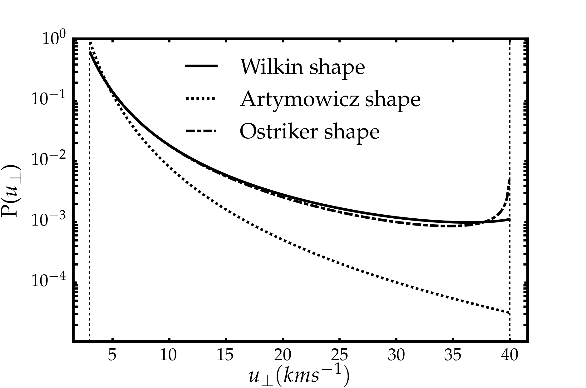
Figure 2: Statistical distributions of 1D planar shock along the bow shock obtained for various bow shock shapes. These distributions are dominated by low-velocity shocks.

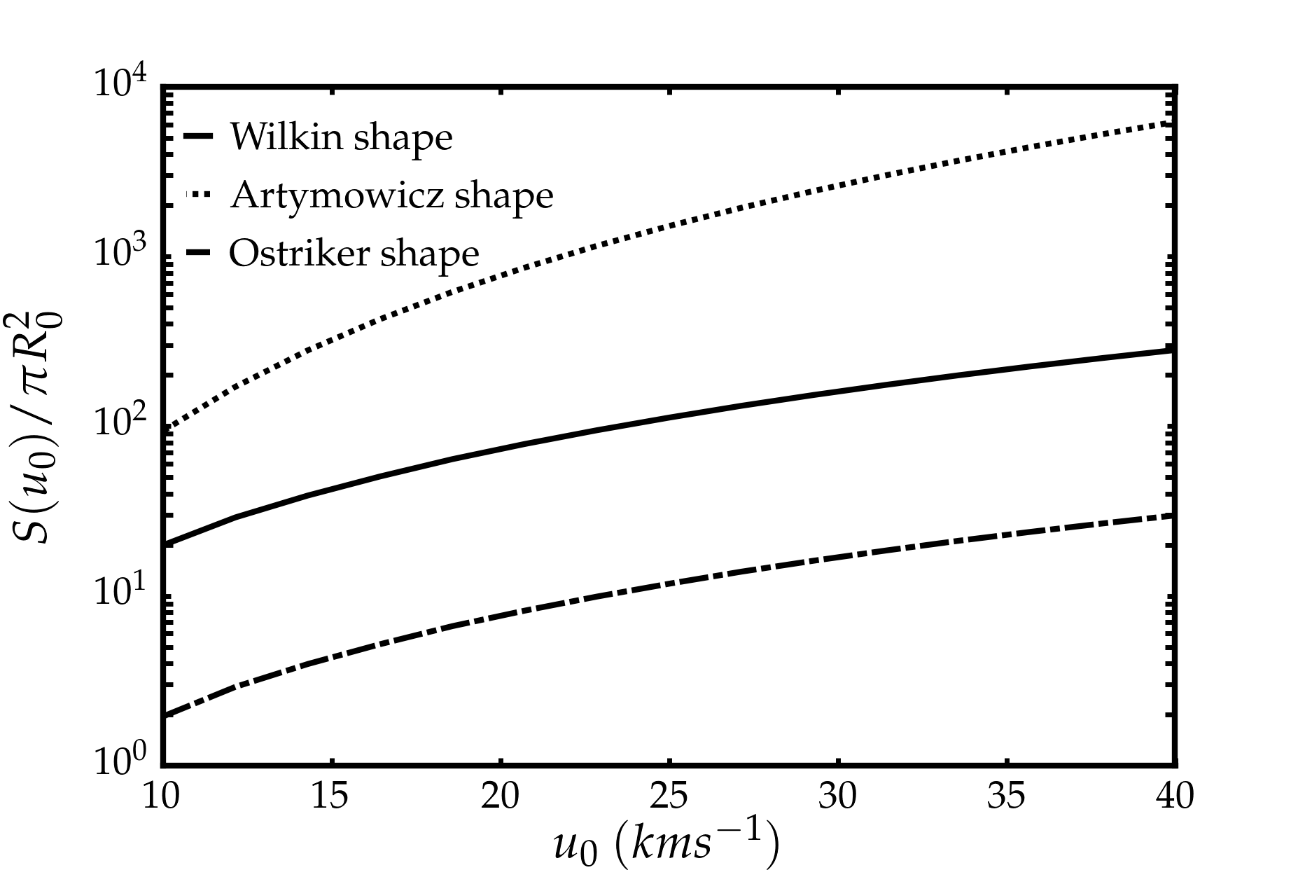
Figure 3: Total surface of the bow shock for various bow shock shapes and terminal velocities, in units of $\pi R_{0}^{2}$ where $R_{0}$ is the length-scale parameter of the bow (on the order of the nose’s curvature radius).

2.3 Example of bow shock shapes

In an elegant and concise article, Wilkin (1996) derived an analytical description of the shape of a bow shock around a stellar wind when it is dominated by the ram pressure of the gas. When dust grains control the dynamics of the gas, the main forces are the gravitation pull and the radiation pressure from the star and the shape of the shock should then be very close to the grains avoidance parabola derived in Artymowicz & Clampin (1997). In fact, the ISM is a mixture between gas and dust grains, so the actual bow shock shape should lie in-between.

For the dust dominated case, the bow shock shape is the Artymowicz parabola expressed as $z=\frac{1}{4R_{0}}x^{2}-R_{0}$ with $R_{c}=2R_{0}$ the curvature radius at apex, $R_{0}$ being the star-apex distance. In the gas dominated case, the bow shock shape follows the Wilkin formula $R=\frac{R_{0}}{\sin\theta}\sqrt{3}\sqrt{1-\theta\cot\theta}$ with $R_{c}=5/4R_{0}$ the curvature radius.

Finally, in the case of the tip of a jet, Ostriker et al. (2001) showed that the shape of the bow shock should be cubic $z=x^{3}/R_{0}^{2}-z_{j}$ with an infinite curvature radius (and $R_{0}$ and $z_{j}$ are length-scales parameters). Figure 3 displays the distributions obtained for various bow shock shapes. Note that low-velocity shocks (u_⊥ $\leq$ 15 km s^-1) always dominate the distribution: this stems from the fact that the corresponding surface increases further away from the axis of symmetry, where entrance velocities decrease. The distribution for the cubic shape has a spike due to its flatness (infinite curvature radius) near the apex. The Wilkin shape has a cubic tail but a parabolic nose. In figure 3 we display the dimensionless surface $S/\pi R_{0}^{2}$ where $S$ is the total surface of the bow shock. $R_{0}$ is an estimate of the radius of the nose of the bow. For elongated shapes such as the parabolic shape, the total surface can be much bigger than the nose cross-section $\pi R_{0}^{2}$. We will subsequently essentially consider an ambient shock with a parabolic shape (Artymowicz shape), unless otherwise stated.

2.4 Orientation of the magnetic field

The magnetic field decouples the ions from the neutral fluid in the shock. However, as discussed in Smith (1992), the effective magnetic field is the component of the field parallel to the shock surface. If the homogeneous pre-shock density is $n_{H}$, the strength scale factor of the ambient uniform magnetic field is defined as $b_{0}=B_{0}(\mu G)/\sqrt{n_{H}[cm^{-3}]}$. The component of the field parallel to the working surface $b_{\parallel}$ is given by

$$\left(\frac{b_{\parallel}}{b_{0}}\right)^{2}=\cos^{2}\alpha\sin^{2}(\varphi-\phi)+[\sin\psi\sin\alpha+\cos\psi\cos\alpha\cos(\varphi-\phi)]^{2}$$ (8)

where the angles $\alpha$ and $\varphi$ monitor the position in the bow shock (this expression is actually valid regardless of the bow shock shape). Figure 4 displays how this component ($b_{\parallel}$) changes along the shock surface in a few cases.

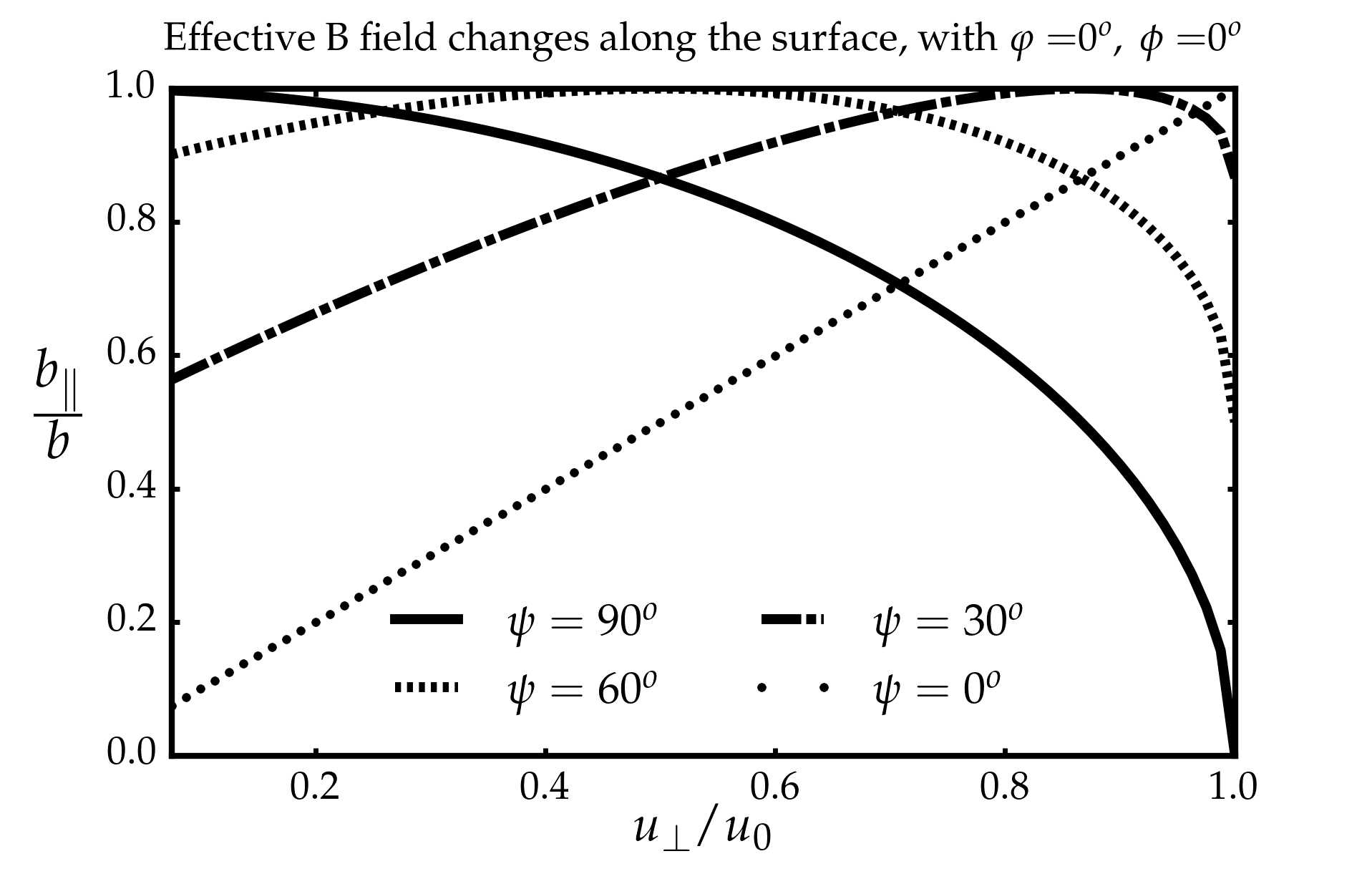
(a)

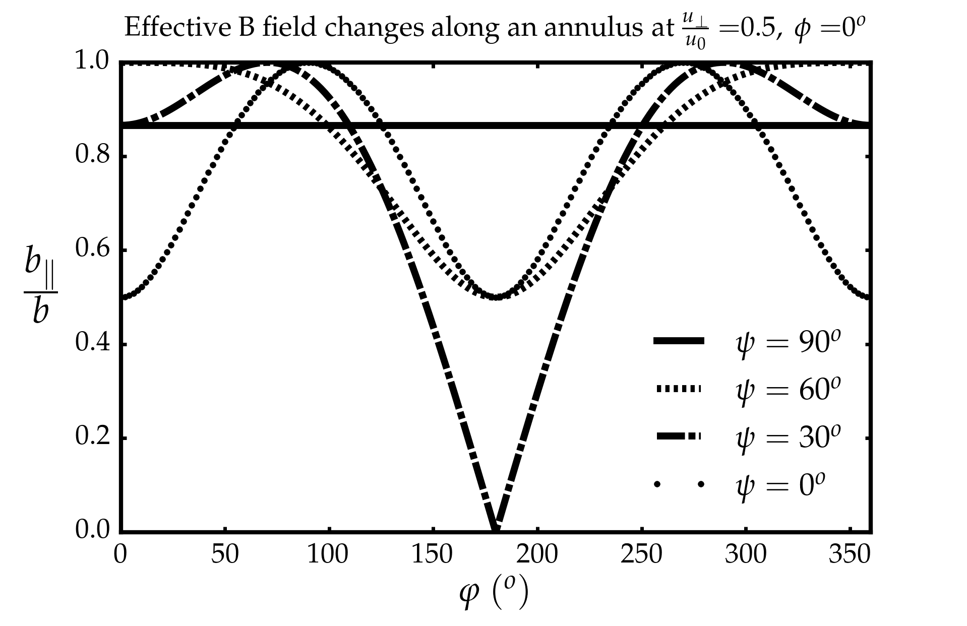
(b)

Figure 4: Variation of the effective transverse magnetic field $b_{\parallel}$ along the bow shock surface: for various directions of b (left) and based on the position of fixed direction of b on an annulus circle (right).

3 1D planar shock models

We now compute the chemical composition and the emission properties of each local planar shock composing a bow shock.

3.1 Grid input parameters

We set all the parameters to values corresponding to typical conditions encountered in the molecular interstellar gas in our Galaxy, as described in table 1. We assume that the ambient gas is initially at chemical and thermal equilibrium and we compute this initial state as in Lesaffre et al. (2013) by evolving the gas at constant density during $10^{12}/n_{H}$ yr. Our initial elemental abundances in the gas, grain cores and ice mantles are the same in Flower & Pineau des Forêts (2003). We also include PAHs with ratio $n(PAH)/n_{H}=10^{-6}$. The irradiation conditions are for a standard external irradiation field ($G_{0}=1$) but an additional buffer of $A_{v0}=0.1$, $N_{0}({\rm H}_{2})=10^{20}$cm^-2 and $N_{0}(CO)=0$ cm^-2 is set between the source and the shock so that the gas is actually mainly molecular (see Lesaffre et al., 2013, for details). In our calculations, the atomic hydrogen fractions $n(H)/n_{H}$ are $7.85\ 10^{-2}$, $5.94\ 10^{-4}$ and $5.89\ 10^{-6}$: they correspond to pre-shock gas densities of $10^{2}$, $10^{3}$ and $10^{6}\ cm^{-3}$, respectively. These initial conditions at steady state are then used as pre-shock conditions to compute the grid of planar shock models.

Our grid of models has a range of shock velocities between 3 to 40 km s^-1 as in Lesaffre et al. (2013), with a velocity step of $\Delta u=1$ km s^-1. However, we take into account the effect of the finite shock age by taking snapshots at 5 different values of age: $10^{2}$, $10^{3}$, $10^{4}$, and $10^{5}$ years for a density of $n_{H}=10^{2}\leavevmode\nobreak\$cm^-3, and a hundred times shorter for a density of $n_{H}=10^{4}\leavevmode\nobreak\$cm^-3. Note that the typical time to reach the steady-state in a C-type shock with $G_{0}=1$ is about $t_{s}=10^{6}$yr$/(n_{H}/10^{2}\mbox{cm}^{-3})$ (with little or no magnetic field dependence, see Lesaffre et al., 2004a).

The projected value of the magnetic field parallel to the shock $B_{\parallel}$ varies along the shock surface, so we need to sample the range of attainable values in our grid. The first constraint for a shock to exist is that its entrance velocity $u_{\bot}$ should be greater than the Alfvén velocity $v_{A}=\frac{B_{\parallel}}{\sqrt{4\pi\rho}}\simeq b_{\parallel}\,1.85\,$km s^-1 where we defined the dimensionless value of the transverse magnetic field using the standard scaling $b_{\parallel}=B_{\parallel}/\mu$G$/(n_{H}/{\rm cm}^{-3})^{1/2}$. The condition $u_{\bot}>v_{A}$ translates as $b_{\parallel}<u_{\bot}/1.85$km s^-1, and we use as upper limit of our grid $b_{\parallel}<b_{\parallel{\rm max}}=u_{\bot}$/3 km s^-1 (see figure 6).

Another important parameter is the magnetosonic speed in the charged fluid $v_{m}=\sqrt{c^{2}_{s}+B_{\parallel}^{2}/4\pi\rho_{c}}$ (where $c_{s}$ and $B^{2}/4\pi\rho_{c}$ are the speed of sound and the Alfvén speed of the charged fluid). The magnetosonic speed is the fastest signal speed in a partially ionized medium. Due to the low ionization degree in the molecular ISM, it is almost proportional to the local magnetization parameter: $v_{m}\simeq B_{\parallel}^{2}/4\pi\rho_{c}=b_{\parallel}v_{m1}$ where $v_{m1}$ is the magnetosonic speed obtained when the magnetization parameter is equal to unity. In our calculations, we find $v_{m1}=18.5$ km s^-1 or $v_{m1}=19.2$ km s^-1 for respective densities of $n_{H}=10^{2}\ cm^{-3}$ or $n_{H}=10^{4}\ cm^{-3}$. The charged fluid mass is dominated by the dust grains: the gas-to-dust ratio turns out to be $\rho/\rho_{d}=180$ for the cores and mantle composition used in our simulations.

3.2 J- and C-type shocks at early age

Depending on the value of the entrance speed relative to the entrance magnetosonic speed $v_{m}$, one can consider different kinds of shocks. When the magnetic field is weak and/or when the ionization fraction is large, the shocks behave like hydrodynamic shocks with an extra contribution from the magnetic pressure. Such shocks are faster than the signal speed in the pre-shock medium. Therefore, the latter cannot "feel" the shock wave before it arrives. Across the shock front, the variables (pressure, density, velocity, etc.) of the fluid vary as a viscous discontinuity jump (the so-called $J$-type shock). When the ionization fraction is small, the magnetosonic speed $v_{m}$ in the charges can be greater than the shock entrance velocity, then a magnetic precursor forms upstream of the discontinuity where the charged and neutral fluids dynamically decouple. The resulting friction between the two fluids heats up and accelerates the neutral fluid. At early ages, the shock is actually composed of a magnetic precursor and a J-type tail (it is a time-dependent CJ-type shock). Chièze et al. (1998) remarked that time-dependent shocks looked like steady-state: this yielded techniques to produce time-dependent snapshots from pieces of steady-state models (Flower & Pineau des Forêts, 1999; Lesaffre et al., 2004b). We follow the approach of Lesaffre et al. (2004b) in the large compression case. The J-type front in a young C-type shock is thus inserted when the flow time in the charged fluid is equal to the age of the shock. The J-type shock ends when the total neutral flow time across the J-type part reaches the age of the shock (the same holds for young J-type shocks). As the shock gets older, the magnetic precursor grows larger and the velocity entrance into the J-type front decreases due to the ion-neutral drag. As a result, the maximum temperature at the beginning of the J-type front decreases with age, as illustrated in figure 6. If the magnetic field is strong enough, the J-type tail eventually disappears and the shock becomes stationary. The resulting structure forms a continuous transition between the pre-shock and the post-shock gas (a stationary C-type shock).

For each value of the entrance velocity $u_{\bot}$, we compute five CJ-type shock models with varying transverse magnetic field $b_{\\ }$ equally spaced between 0 and $u_{\bot}/v_{m1}$, and we compute five J-type shocks models with varying transverse magnetic field $b_{\\ }$ equally spaced between $u_{\bot}/v_{m1}$ and $b_{\parallel{\rm max}}=u_{\bot}$/3 km s^-1. That way, we homogeneously sample the possible shock magnetizations that are likely to occur in the 3D bow shock (see figure 6).

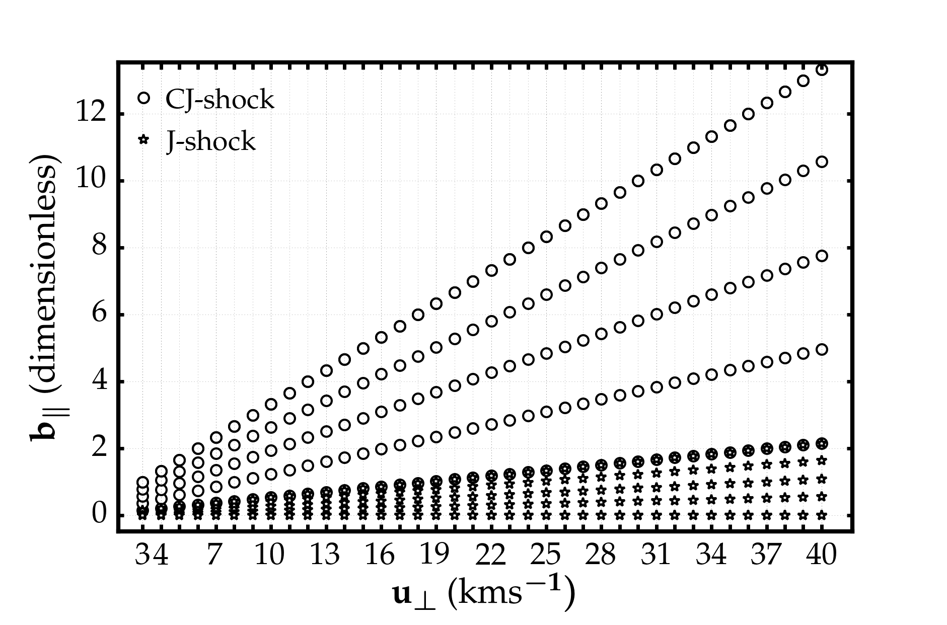
Figure 5: Grid of 1D models in the parameter space $(u_{\bot},b_{\parallel})$.

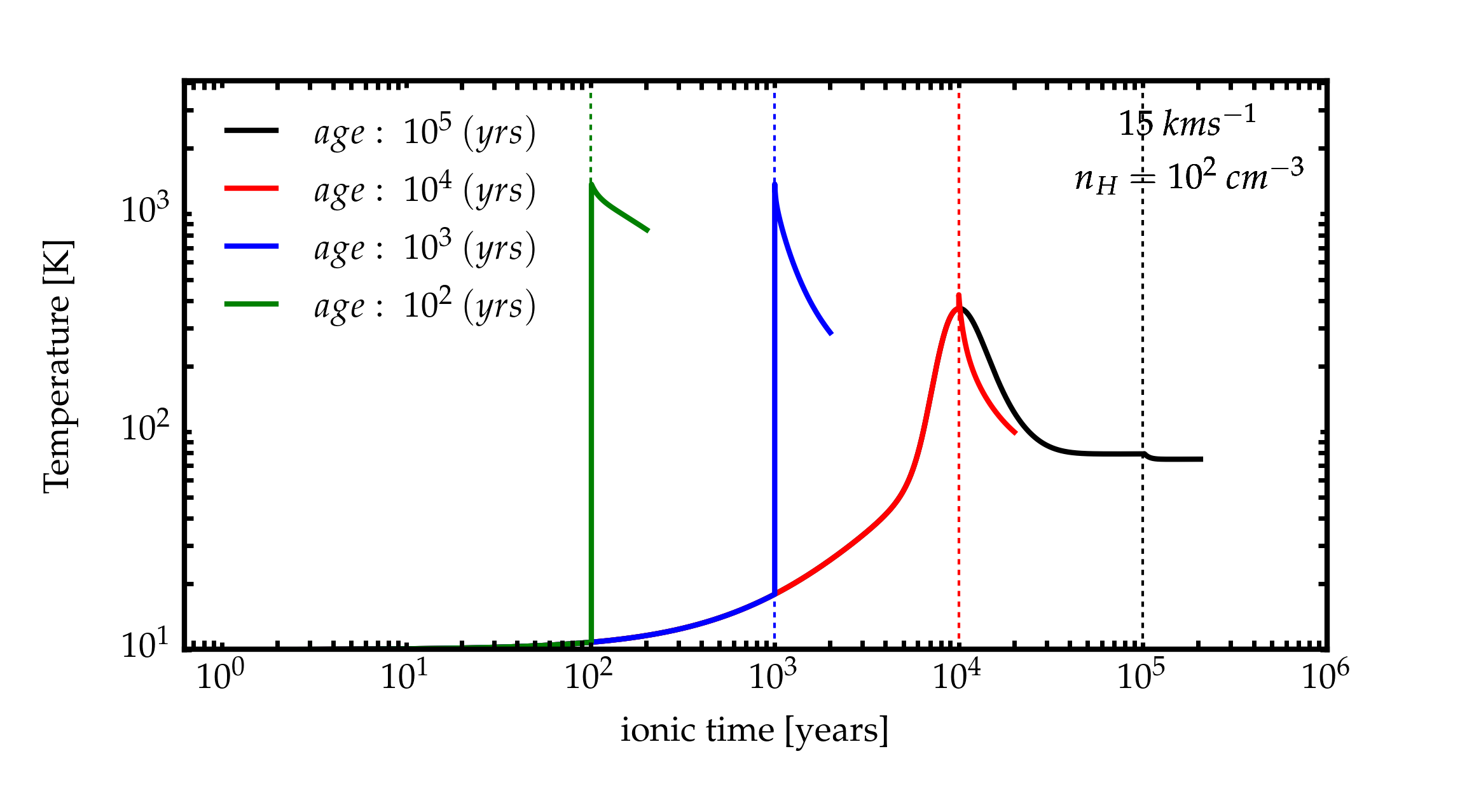
Figure 6: Temperature profile of CJ-type shocks at various shock ages for $n_{H}=10^{2}\ cm^{-3}$ and b=5.

The main input parameters of the model are gathered in table 1.

Parameter	Value	Note
$n_{H}$	$10^{2}$cm-3, $10^{4}$cm-3	Pre-shock density of H nuclei
$A_{\nu}$	0.1	Extinction shield
$N_{0}(H_{2})$	$10^{20}$cm-2	Buffer H2 column density
$N_{0}(CO)$	0 cm-2	Buffer CO column density
$G_{0}$	1	External radiation field
$\zeta$	$3.10^{-17}$ $s^{-1}$	Cosmic ray flux
OPR	3	Pre-shock H2 ortho/para ratio
$u_{\bot}$	$3,4,5,\dots 40$ km s-1	Effective shock velocity
$b_{\parallel}v_{m1}/u_{\bot}$	$0,\dots,1$	Range of $b_{\parallel}$ parameter for J-type shocks
$b_{\parallel}v_{m1}/u_{\bot}$	$1,\dots,\frac{v_{m1}}{3\mbox{km\ s}^{-1}}$	Range of $b_{\parallel}$ parameter for CJ-type shocks
age $\times n_{H}/$100 cm${}^{-3}/$yr	$10^{2}$, $10^{3}$, $10^{4}$, $10^{5}$	Shock age

Table 1: Main input parameters of model.

3.3 H₂ excitation in C- and J-type shocks

An H₂ ro-vibrational level $(v,J)$ can be populated after a collision with another species provided that the temperature yields more energy per particle than the energy level $E_{vJ}$. In a J-type shock, the sudden surge of viscous heat in the adiabatic shock front easily leads to large temperatures ($T_{J}=53K(u/$km s${}^{-1})^{2}$, see Lesaffre et al. (2013), equation 10) which are able to excite high energy levels. Figure 7(a-b) show the level populations for young ages, where even CJ-type shocks are dominated by their J-type tail contribution. These figures illustrate the threshold effect for two different energy levels: their population rises quickly and reaches a plateau when $u>u_{vJ}$, with $u_{vJ}$ a critical velocity depending on the energy level. Note the weak dependence of the plateau on the shock magnetization for J-type shocks, as magnetic pressure only marginally affects their thermal properties. The critical velocity $u_{vJ}$ mainly depends on the energy level ($E_{vJ}\simeq k_{B}T_{J}$) and only weakly depends on the magnetization.

On the other hand, C-type shocks dissipate their energy through ion-neutral friction, a process much slower than viscous dissipation: at identical velocity, C-type shocks are much cooler than J-type shocks, but their thickness is much larger. C-type shocks dominate the emission of old CJ-type shocks, when the J-type front contribution almost disappears (figure 7c of the ’o’ symbols). Due to their low temperature, high energy levels can never be populated (figure 7d). This enhances the threshold effect, with a discontinuous jump at $u=bv_{m1}$. On the contrary, energy levels of energy lower than $k_{B}T_{C}$, with $T_{C}$ the typical temperature of a C-type shock, will be much more populated in a C-type shock than in a J-type shock due to the overall larger column-density. This is illustrated in the figure 7c for a low energy level. The discontinuous jump at $u=bv_{m1}$ becomes a drop instead of a surge and a peak appears in the level population. Magnetization in C-type shocks controls the compressive heating which, in turn, impacts the temperature: excitation of H₂ low-energy levels in C-type shocks decreases systematically with larger magnetization, but the effect remains weak within C-type shocks. However, the magnetization is important insofar as it controls the transition between C-type and J-type shocks, which have very different emission properties.

To summarize, at a density of $n_{H}=10^{2}$/cm³, the excitation of a given H₂ level follows a threshold in velocity after which a plateau is reached, with little or no magnetic field dependence. However, low energy levels at old ages, for velocities below the magnetosonic speed, can be dominated by C-type shock emission. In that case, the H₂ level population peaks at the magnetosonic speed before reaching a plateau. Therefore, H₂ emission in bow shocks is likely to be mostly dominated by J-type shocks.

At high density, the picture is essentially unchanged, except for the effect of H₂ dissociation which is felt when the velocity is larger than the H₂ dissociation velocity: the value of the plateau decreases beyond this velocity (see the right half of each panel in figure 8, which is in other respects similar to figure 7). At even higher densities, H₂ dissociation completely shuts off H₂ emission in J-type shocks, and we reach a situation where the bow shock emission is dominated by C-type shocks, as in Gustafsson et al. (2010).

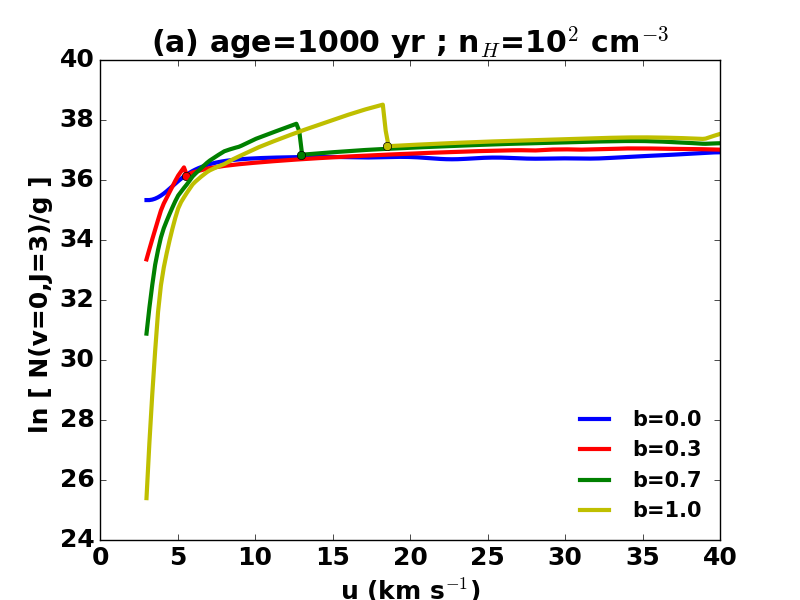
(a)

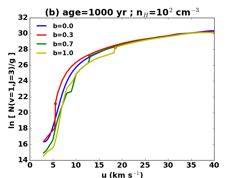
(b)

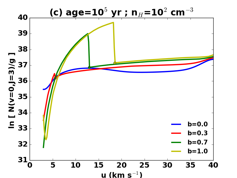
(c)

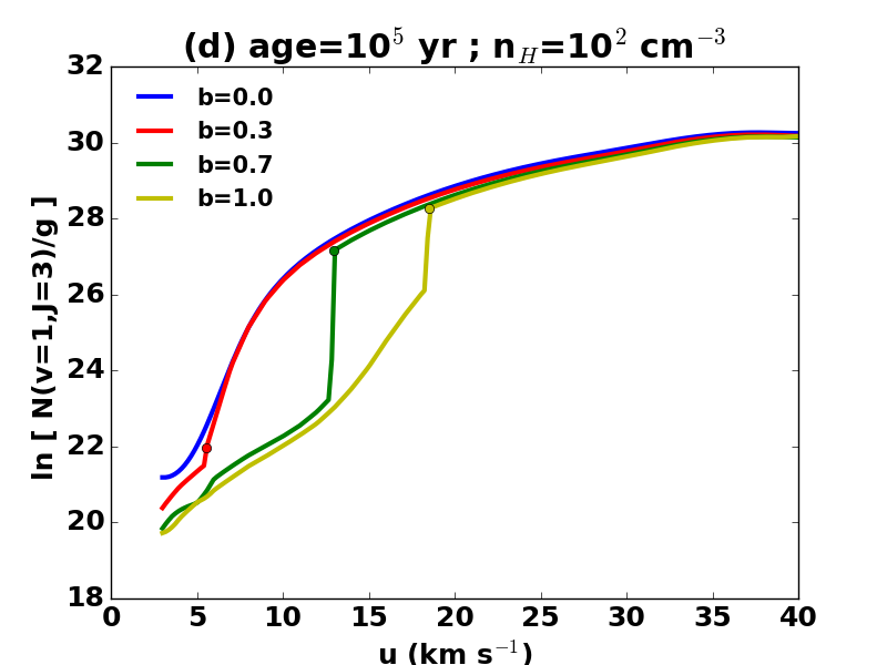
(d)

Figure 7: Overview of results from our models for a pre-shock density $n_{H}=10^{2}$/cm³. We show the natural logarithm of the integrated column-densities of H₂ populations normalized by their statistical weight. They are given as a function of the velocity $u$ for various values of the magnetic field parameter $b_{\parallel}$. Left panels are for the level $(v,J)=(0,3)$, the upper level of the 0-0S(1) line and the right panels are for the level $(v,J)=(1,3)$, the upper level of the 1-0S(1) line. Upper panels are for a young age of 10³ yr while bottom panels are nearly steady-state at an age of $10^{5}$ yr. In each panel, the symbol ’o’ marks the transition between CJ-type shocks (on the left-hand side) and J-type shocks (on the right hand side), when the velocity $u$ is equal to the magnetosonic speed $bv_{m1}$.

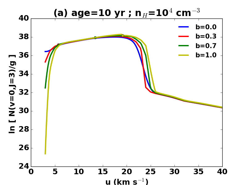
(a)

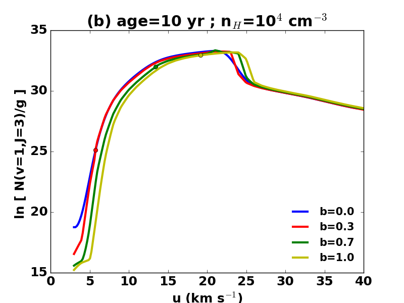
(b)

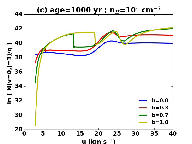
(c)

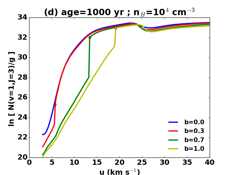
(d)

Figure 8: Same as 7 but for the denser case $n_{H}=10^{4}$/cm³. The corresponding ages are: upper panels at a young age of 10 yr while the bottom panels are nearly steady-state at an age of $10^{3}$ yr.

4 3D bow shock models

In this section, we combine the grid of planar shocks and the statistics of planar shock velocity $u_{\bot}$ computed in the previous sections to produce observable diagnostics of 3D bow shocks.

4.1 H₂ excitation diagram

4.1.1 Excitation of a given H₂ level

The average column-density of a given excited level of H₂ along the bow shock can be expressed as:

$$N^{\rm tot}_{vJ}(age,u_{0},b_{0},\psi)=\int_{0}^{2\pi}\frac{d\varphi}{2\pi}\int_{c_{s}}^{u_{0}}P_{u_{0}}(u_{\bot})N_{vJ}(age,u_{\bot},b_{\parallel})du_{\bot}$$ (9)

where $P_{u_{0}(u_{\bot})}$ is the distribution computed in section 2 and $N^{\rm tot}_{vJ}$ and $N_{vJ}$ are the column-densities of H₂ in the excited level $(v,J)$ in the whole bow shock and in each planar shock, respectively.

As noted in section 3.3, $N_{vJ}$ sharply increases as a function of $u_{\bot}$ at a given threshold velocity $u_{vJ}$ before reaching a plateau. We also showed that the statistical distribution was steeply decreasing as a function of $u_{\bot}$. As a result, the product of the two peaks at around $u_{vJ}$ and its integral over $u_{\bot}$ is a step function around $u_{vJ}$ (see figure 9). This situation is reminiscent of the Gamow peak for nuclear reactions. Then, $N^{\rm tot}_{vJ}(u_{0})$ tends to a finite value when $u_{0}$ is much greater than the threshold velocity $u_{vJ}$. The final value depends both on magnetization and age.

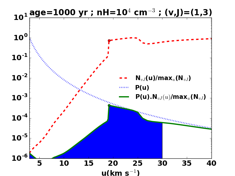
Figure 9: Illustration of the “Gamow-peak” effect on the integration of the total column densities of the H₂ level $(v,J)=(1,3)$ in a bow shock with terminal velocity $u_{0}=30$ km s^-1, $n_{H}=10^{2}$/cm³, and the age is 10⁵ yr.

4.1.2 Resulting H₂ excitation diagram

The excitation diagram displays the column densities in each excited level (normalized by their statistical weight) as a function of their corresponding excitation energy. This is an observational diagnostic widely used to estimate the physical conditions in the emitting gas.

Figure 10a shows the influence of the terminal velocity on the excitation diagrams of H₂ at an age of $10^{4}$ yr. As expected, the excitation diagram saturates at large velocity, when $u_{0}$ is larger than all the individual $u_{vJ}$ of the levels considered. That saturation occurs quicker at low energy levels, as the corresponding critical velocity is lower.

Figure 10b illustrates the effect of density on the excitation diagram. Roughly speaking, the column-densities are proportional to the density, but in this example (40 km s^-1 bow shock), higher energy levels are subject to H₂ collisional dissociation, and they are slightly less populated relative to their low energy counter part.

At young ages, shocks are dominated by the emission properties of J-shock: as time passes, C-type shocks increase the emission of low energy levels and the excitation diagram of the bow shock is slightly steeper at the origin (figure 10c). Interestingly, the energy level just above 2000K does not seem to be affected by age (it is also weakly affected by all the other parameters, the safe density) and all the curves converge on this point.

As mentioned in section 2.3, the shape of bow shocks affects the velocity distribution and the relative weight between of the large velocities increases when one moves from a parabola to a Wilkin shape. As a result, a bow shock with a Wilkin shape has more excited high energy levels than a parabolic bow shock (figure 10d).

Finally, the magnetic field tends to shift the transition between C-type and J-type shocks in the bow shock to larger velocities. At early age, it does not matter much, since both C-type and J-type shocks are dominated by J-type shock emission. At later ages, though, the low energy levels get an increasing contribution from C-type shocks and see their excitation increase. Conversely, high energy levels are less excited because the overall temperature of the shock decreases, as seen on figure 10e. The orientation of the magnetic field azimuthally affects the range of values of $b$ (as $\varphi$ varies) but its main systematic effect is to shift the magnetization from low velocities to large velocities as it gets more and more parallel to the axis of symmetry (figure 4). Figure 10f shows the differential effect caused by varying the angle $\Psi$: tending $\Psi$ to 0^o amounts to increasing $b$ (high energy levels are less excited, whereas low energy levels are more excited). The resulting change is subtle but we show below that it might still be probed by observations.

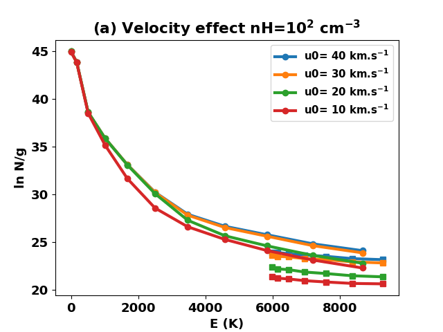
(a)

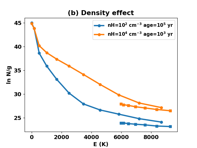
(b)

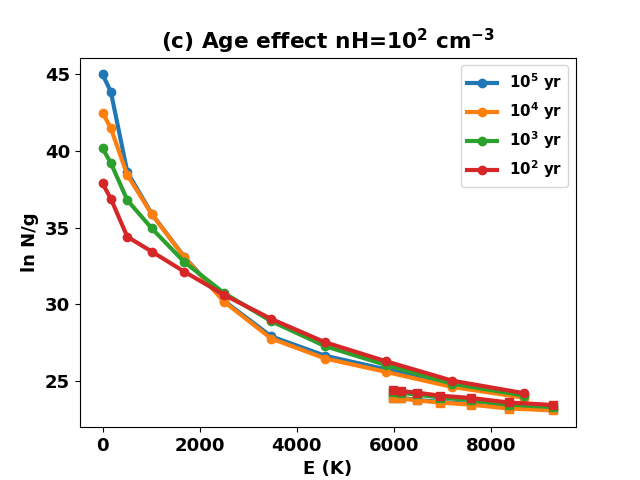
(c)

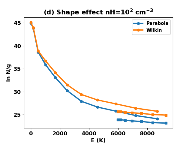
(d)

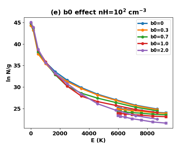
(e)

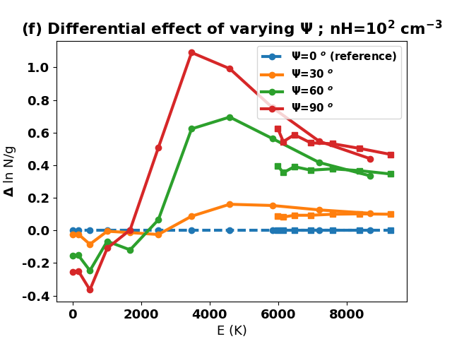
(f)

Figure 10: Excitation diagrams of H₂ showing the effect of varying some of the parameters of the model. The reference model is nH=1e2/cm3, age=1e5 yr, b0=1, Psi=0, shape=Parabola, u0=40 km s^-1. It is always displayed in solid blue. Connected circle symbols have all $v=0$ (pure rotational levels) while square symbols have $v=1$.

4.1.3 Using 1D models to fit 3D excitation diagrams

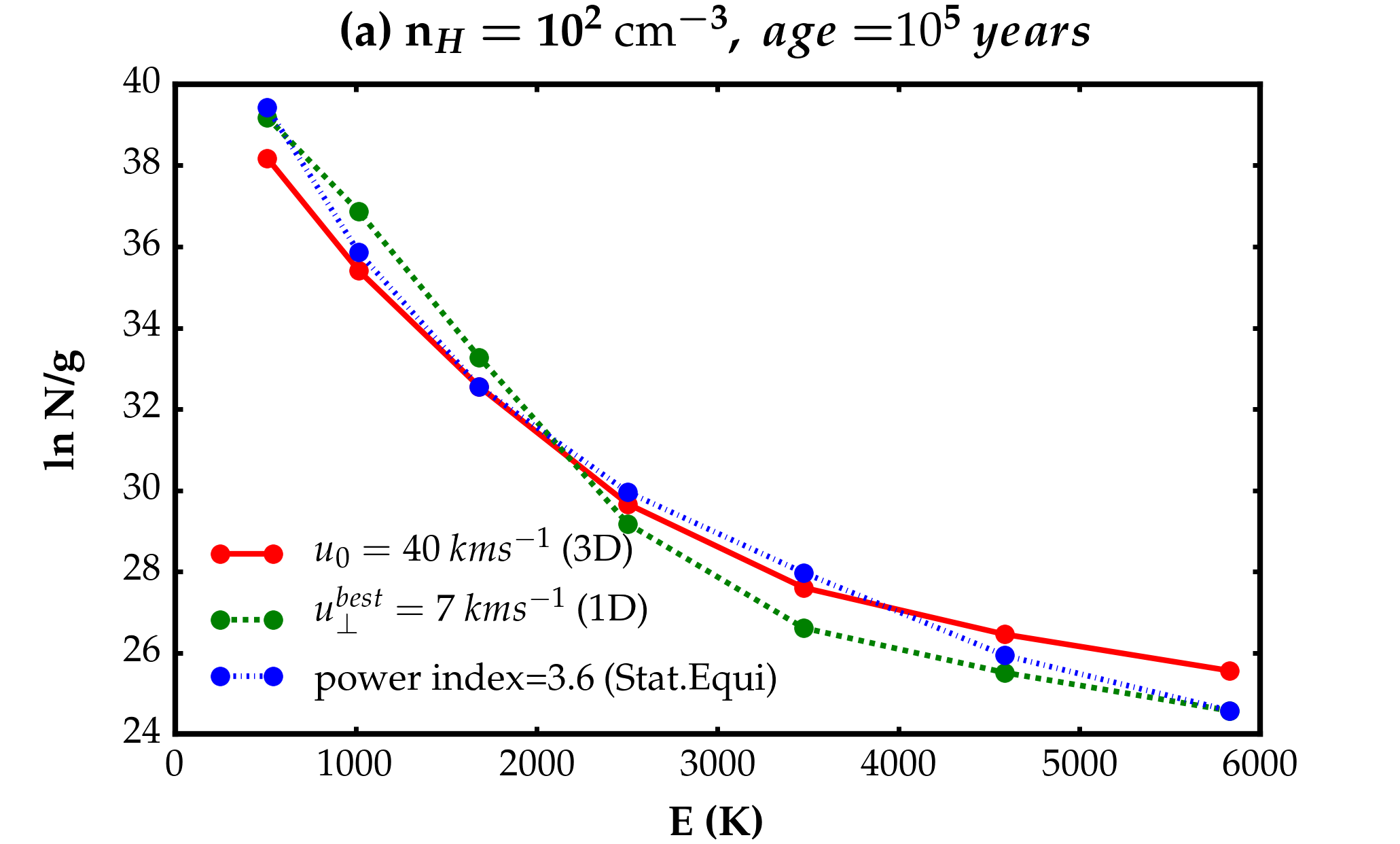
(a)

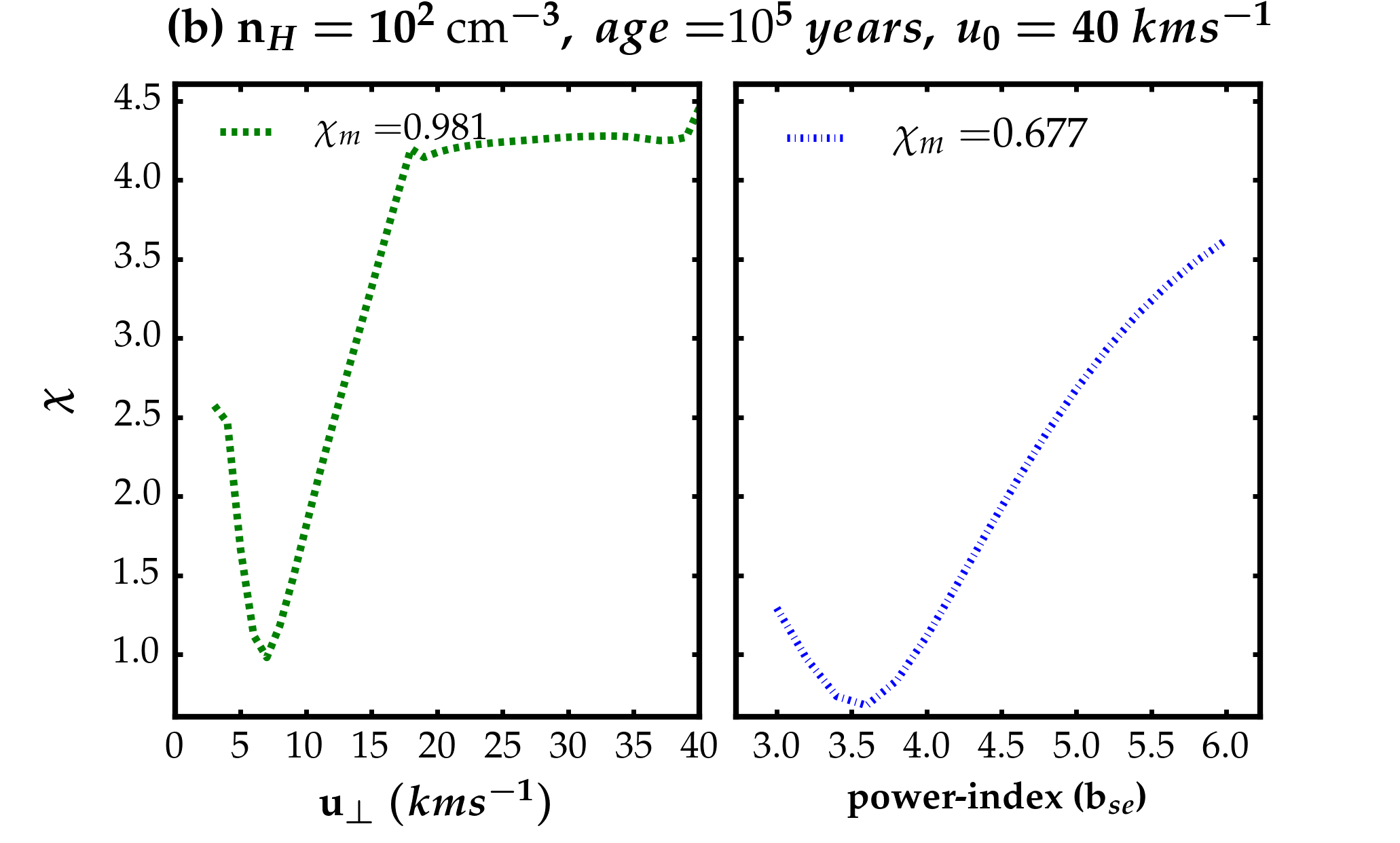
(b)

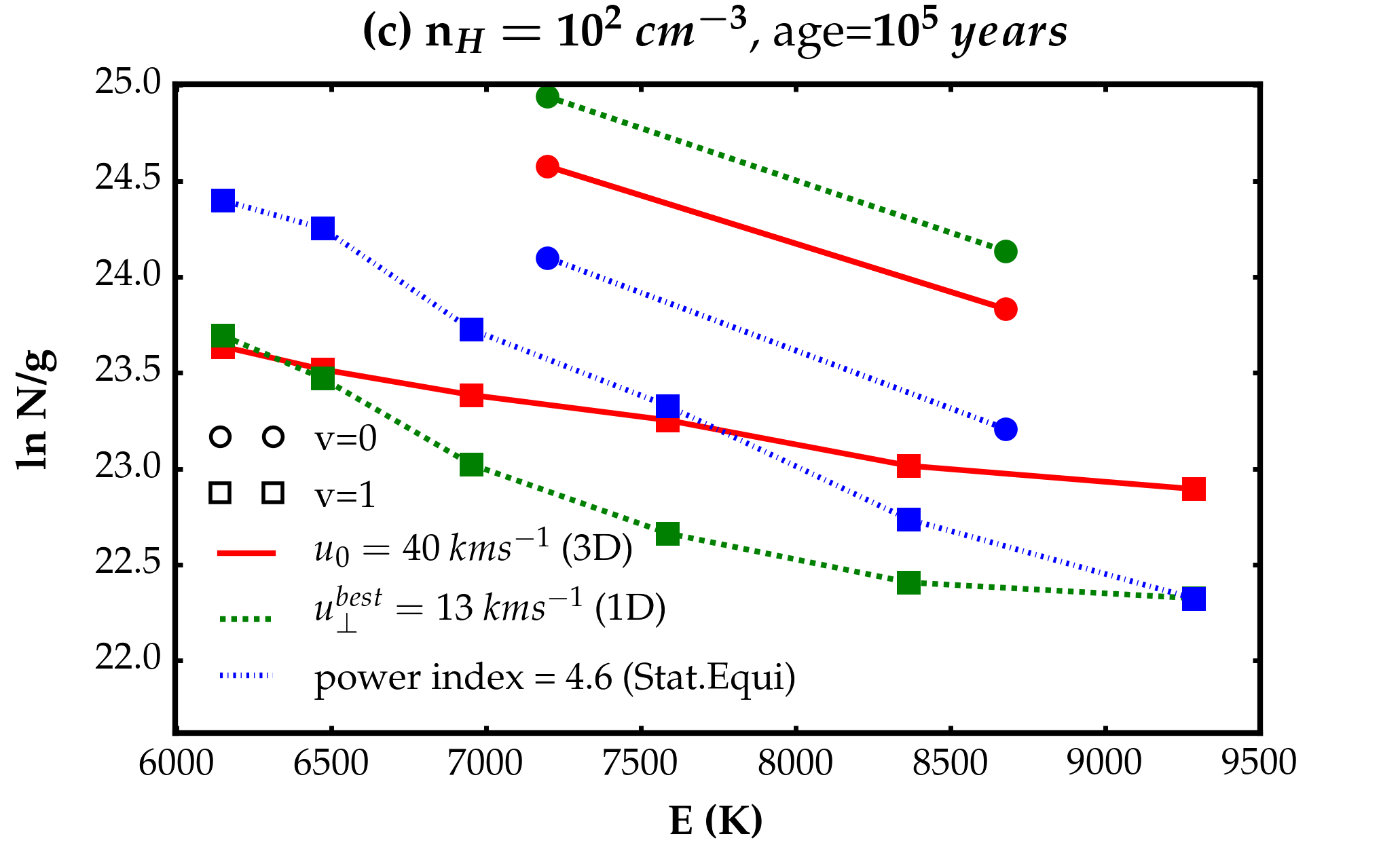
(c)

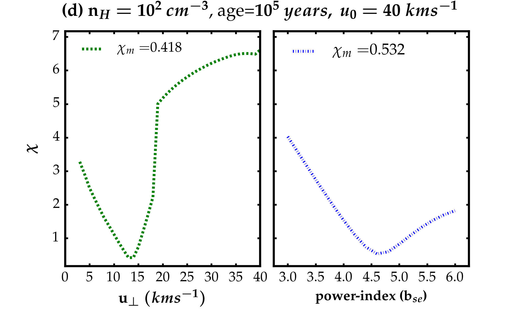
(d)

Figure 11: Results of the fit of 1D models and statistical equilibrium approximations to a 3D bow shock. (a-b) Transitions with upper level $E_{vj}<5900\leavevmode\nobreak\$K (JWST-like) are used. (c-d) Fitted transitions have 5900 K$<E_{vj}<10\,000\leavevmode\nobreak\$K. (a-c) Comparison of the excitation diagrams of the bow shock to the best 1D fit and the best NY08 fit, (b-d) standard deviation of the natural logarithm difference between the two diagrams ($\chi=\sqrt{\chi^{2}}$) as the entrance velocity in the 1D model and the power-index in NY08 assumption vary. The bow shock parameters are: pre-shock density $10^{2}\ cm^{-3}$, $b_{0}=1$, $\psi=90^{o}$, and the age is 10⁵ yr. Connected circle symbols all have $v=0$ (pure rotational levels) while square symbols have $v=1$.

Observations often consider low energy transitions (pure rotational or low vib-rotational levels): although we included the first 150 levels in our calculations, here we mainly consider the levels with an energy up to $10^{4}$K. The two lowest rotational states (J=0 and 1) are, of course, unobservable in emission. The James Webb Space Telescope (JWST) will observe pure rotational transitions up to energies of about 5900K (seven levels involved). This is similar to the performances of its predecessors: the Infrared Space Observatory (ISO) and the Spitzer telescope. These two infrared telescopes have been used to observe shocked regions, generate excitation diagrams and maps around Young Stellar Objects (YSOs) (e.g., Giannini et al. 2004; Neufeld et al. 2009) or supernova remnants (SNRs) (e.g., Cesarsky et al. 1999; Neufeld et al. 2014) shocks. The AKARI mission has also been used for similar purposes in SNRs environments (e.g., Shinn et al. 2011). In addition, note that the JWST will also target rovibrational transitions. Finally, the Echelon-Cross-Echelle Spectrograph (EXES, operating between 4.5 and 28.3 microns, DeWitt et al. 2014) onboard the Stratospheric Observatory For Infrared Astronomy (SOFIA) should allow observations of pure rotational transitions of H₂, but no program has been explicitely dedicated to the observation of shocked H₂ with this instrument so far.

Most observations are unable to resolve all details of a bow shock, and the beam of the telescope often encompass large portions of it, therefore mixing together planar shocks with a large range of parameters. However, it is customary to use 1D models to interpret observed excitation diagrams. Previous work (Neufeld & Yuan 2008, hereafter NY08; Neufeld et al. 2009; Neufeld et al. 2014) have also shown that statistical equilibrium for a power-law temperature distribution T${}^{-b_{SE}}$ dT can be quite efficient at reproducing the observed H₂ pure rotational lines. We thus seek to explore how accurately these two simple models perform as compared to 3D bow shocks. We consider the worst case scenario where the whole nose of a parabolic bow shock is seen by the telescope: the effective entrance velocity $u_{\bot}$ varies from the speed of sound $c_{s}$ (in the wings of the bow shock) to the terminal velocity $u_{0}$ (at the apex of the bow shock).

The following $\chi$ function is used to estimate the distance between 1D and 3D models:

$$\chi^{2}=\frac{1}{L}\sum_{vj}[\ln(\frac{N^{\rm tot}_{vj}}{g_{vj}})-\ln(\frac{N^{u_{\bot}}_{vj}}{g_{vj}})-C]^{2}$$ (10)

with $L$ the number of observed vib$\_$rotational levels $(v,j)$, and $g_{vj}$ the statistical weight of each level $(v,j)$. The constant $C$ reflects the fact that the beam surface at the distance of the object may not match the actual emitting surface of the bow-shock, partly because of a beam filling factor effect and partly because the bow-shock surface is curved. We assume here that the observer has a perfect knowledge of the geometry and we take $C=0$, which means that the 1D shock model has the same surface as the 3D bow-shock to which it is compared with. The best 1D model and power-law assumption selected is the one yielding the smallest $\chi^{2}$ value on our grid of 1D models.

Figure 11 shows the result of the fit on a 30 km s^-1 bow shock at age $10^{5}$ years, density $n_{H}=10^{2}$ cm^-3, and magnetization parameter $b_{0}=1$ ($\Psi=90^{o}$). 1D models have the same parameters (same age, pre-shock density and $b_{\parallel}=1$) except the entrance velocity $u_{\bot}$. We find that the best velocity is either 8 or 13 km s^-1 depending on the range of lines considered. This is way below the terminal velocity and this illustrates again the fact that the resulting 3D excitation diagram is dominated by low velocity shocks. As a consequence, the use of higher energy lines reduces the bias, and a cubic shape for the bow shock yields less bias towards low velocity than a parabolic shape (not shown here). In the left hand sides of the panels (b)-(d), the resulting $\chi^{2}$ is around one in all cases: it corresponds to an average mismatch of about a factor of 3 between the 3D and 1D column-densities, a common result when comparing 1D models and observations.

Figure 12 systematically explores this bias as a function of the bow shock terminal velocity: the best 1D model usually has an entrance velocity smaller than the terminal velocity of the 3D bow-shock. Moreover, when the 3D excitation diagram saturates at large $u_{0}$, the best 1D model does not change.

Following the approach of NY08, we calculate the H₂ levels population in statistical equilibrum for a range of temperatures (100K to 4000K) and convolve this with a power-law distribution of the gas temperature. We explore power-indices ($b_{SE}$) varying from 3 to 6 (as in NY08) in steps of 0.2. We recover the fact that the NY08 approximation performs very well in the low energy regime of pure rotation. In the case displayed in figure 11(a), our best fit power-index is 3.6, close to the estimation of 3.78 for parabolic bow-shocks calculated by equation (4) in NY08. However, figure 11(c) shows that this simple approach fails for vibrational levels, or rotational levels of higher energy.

We then turn on recovering magnetization from 1D models. We first fix the terminal velocity of the bow shock to $u_{0}=40$ km s^-1 and explore several values of the magnetization $b_{0}$, while keeping $\Psi=90^{o}$. Once the best matching 1D velocity is found, we further let the magnetization parameter $b_{\\ }$ of the 1D model vary freely and explore which value best fits the 3D model (while keeping $u_{\bot}$ fixed). The result of this second adjustment is shown in figure 13: the magnetization parameter of the best 1D model is only slightly below and represents a good match to the original magnetization parameter of the bow shock. Next, we assume that a priori information about the bow shock velocity (usually by looking at some molecular line width, for example) is available. We now fix $b_{0}=1$ for the underlying 3D model and assume $u_{\bot}=u_{0}$ in the 1D models while searching for the best $b_{\parallel}$ value. The retrieved magnetization parameter is usually too high, which may lead to overesimations of the magnetization parameter when the dynamics have been constrained independently.

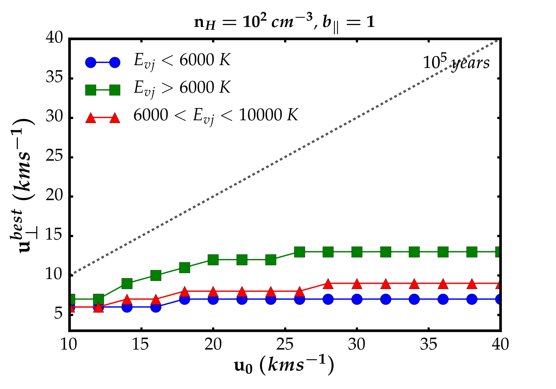
Figure 12: Velocity bias between 1D and 3D model. Blue circle symbols fit only $E_{vj}<5900K(JWST-like)$, the Green square symbols fit only $E_{vj}>5900K$ (ground based) and the red triangles fit $6000<E_{vj}<10000K$. The parameters of the bow shock are the same as for figure 11. The dotted black line is $u^{best}_{\perp}=u_{0}$.

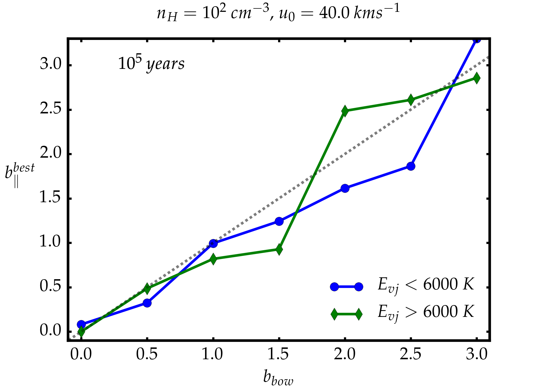
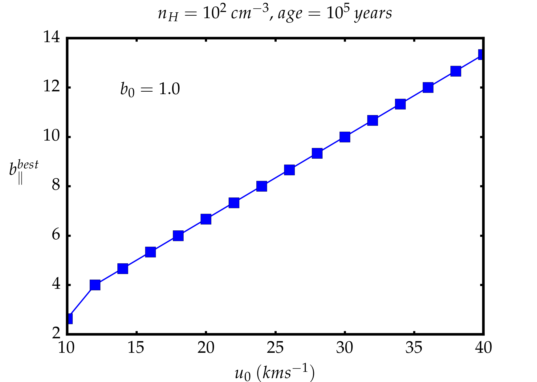
Figure 13: Magnetization bias between 1D and 3D models. The top panel is at $u_{0}=40$ km s^-1 and for each value of $b_{0}$, it gives the best $b_{\parallel}$ after the best $u_{\bot}$ has been determined. The bottom panel is at $b_{0}=1$ and for each value of $u_{0}$, it gives the best matching $b_{\parallel}$ when $u_{\bot}=u_{0}$ is assumed. Symbols are the same as in figure 12. The remaining parameters of the bow shock are the same as for figure 11.

4.1.4 Applications and prospects

In this section, we briefly show how to use the 3D bow shock to interpret and constrain the parameters of bow shock observations.

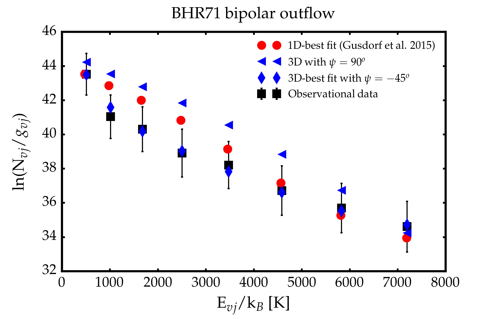
Figure 14: Comparison between BHR71 observations and several bow shock models. Red circles: best fit with the 1D model of Gusdorf et al. (2015), green diamonds: our own corresponding 1D model (a 3D model with velocity close to 22 km s^-1 and $\Psi=90^{o}$ so that the transverse magnetic field is uniform), blue diamonds: best fit with our 3D model (same as the previous model, but with magnetic field orientation $\Psi=-44^{o}$).

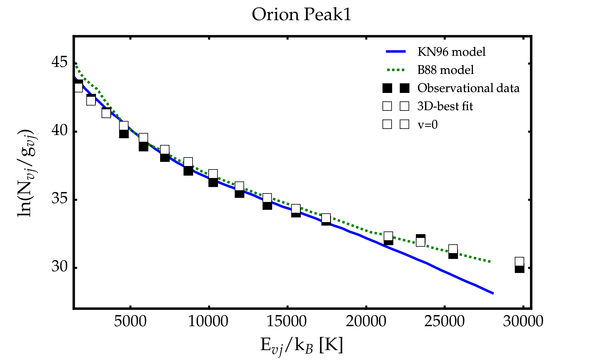
Figure 15: H₂ Excitation diagram observed in OMC-1 Peak1 (Rosenthal et al., 2000) compared with various models: our best-fit 3D-model of bow shock (open symbols), and the best fit models from Rosenthal et al. (2000): a combination of two planar C-shocks models from Kaufman & Neufeld (1996) (KN96) and one J-type shock model from Brand et al. (1988) (B88).

BHR71

Located at a distance of about 175 pc (Bourke et al. 1995), BHR71 is a double bipolar outflow (Bourke et al. 1997; Bourke 2001) emerging from a Bok Globule visible in the southern sky. The two outflows are spectrally distinguishable (Parise et al. 2006). Their driving protostars, IRS 1 and IRS 2 have luminosities of 13.5 and 0.5 L_☉ (Chen et al. 2008) and are separated by about 3400 AU. For this double star system, the time since collapse has been evaluated to about 36000 yr (Yang et al. 2017). Multiple observations of this outflow system have been performed from infrared to sub-millimeter wavelength ranges. Bright HH objects HH320 and HH321 (Corporon & Reipurth 1997) have been detected, as well as chemical enhancement spots (Garay et al. 1998) and several other knots of shocked gas (Giannini et al. 2004). By combining H₂ observations performed by Spitzer (Neufeld et al. 2009; Giannini et al. 2011) and SiO observations obtained from the APEX telescope, Gusdorf et al. (2011) were able to characterize the non-stationary CJ-type shock waves propagating in the northern lobe of the biggest outflow. They more tightly constrained the input parameters of Paris-Durham shock models by means of successive observations of low- to higher-$J_{\rm up}$ CO (Gusdorf et al. 2015) using APEX and SOFIA. The most recent studies based on Herschel observation hint at the presence of an atomic jet arising from the driving IRS1 protostar (Nisini et al. 2015; Benedettini et al. 2017). This does not challenge the existence of a molecular bow-shock around the so-called SiO knot position in the northern lobe of the main outflow, where most attempts have been made to compare shock models with observations (Gusdorf et al. 2011; Gusdorf et al. 2015; Benedettini et al. 2017). In particular, the last three studies have placed constraints on shock models of the H₂ emission over a beam of 24" centred on this position: pre-shock density $n_{\rm{H}}=10^{4}$ cm³, magnetic field parameter $b=1.5$, shock velocity $v_{\rm s}=22\ \rm km\ s^{-1}$, and age of 3800 years. In these studies, the influence of the external ISRF or from the driving protostar was neglected, with an equivalent $G_{0}$ factor set to 0. The excitation diagram that was used can be seen in figure 15, where the large errorbars reflect the uncertainty on the filling factor and the proximity of the targeted region to the edge of the Spitzer-IRS H₂ map.

Here we attempt to reproduce the same H₂ emission data around the SiO knot position as in Gusdorf et al. (2015). To fit a 3D model to this data, we should in principle adjust all the parameters in table 3, which would be a bit tedious, and very likely underconstrained by the observations. Instead, we started up from already published parameters and expanded around these values. We hence use a narrow range of velocities around $u_{0}=22$ km s^-1, $b_{0}=1.5$ and $n_{H}=10^{4}$cm^-3 as indicated by Gusdorf et al. (2015). These authors found an age of 3800 yr, so we took our grid models at an age of 1000 yr, as 10⁴yr would not be compatible with the extent of the shock. A speed of 22 km s^-1 during 1000 yr already results in a shock width of 0.02 pc, about the same size of the beam (24" at 200pc according to Gusdorf et al. (2015)), although the H₂ lines emission region is a factor of a few smaller.

Figure 15 illustrates the comparison between our models and the observational values. We first restrict the velocity range in the bow shock velocity distribution to the narrow interval [21,23] km s^-1 that is close to the original best solution of Gusdorf et al. (2015). This also accounts for the fact that the beam selects a local portion of the bow-shock and one might expect to find a privileged velocity.

First, we examine the case $\Psi=90^{o}$ when the magnetization is close to $b_{0}$ and uniform throughout a transverse annulus of the bow-shock. Technically this is still a 3D model, but it is very close to the model in our grid of planar shocks with similar parameters because we use a very narrow range of velocities combined with uniform magnetization. The excitation diagram for this model is noted as the green diamonds in figure 15. Although it slightly differs from the best model of Gusdorf et al. (2015), it is not much further away from the observational constraints ($\chi=1.0$ in the model in Gusdorf et al. (2015) and $\chi=1.5$ in our model at $\Psi=90^{o}$).

Second, we leave the orientation of the magnetic field $\Psi$ free and we find the best model at $\Psi=-44^{o}$: this greatly improves the comparison with observations ($\chi=0.2$). In particular, the curvature of the excitation diagram that was difficult to model, is now almost perfectly reproduced. At this orientation, the model is a mixture of planar shocks with transverse magnetization between $b_{0}$ and a small minimum value. Because we limited the velocity to such a narrow range, this model is effectively a 2D model.

Third, we checked that increasing the velocity range, changing the shock shape, or limiting the integration range for the angle $\varphi$ (to account for the fact that the observational beam probably intersects only one flank of the bow shock) did not improve the fit: the interpretation capabilities of our 3D model seems to be reached. Table 3 sums up our constraints on the parameters of our model. We estimate 3-$\sigma$ error bars for $\Psi$ by investigating the shape of the $\chi^{2}$ well around the best value: we vary $\Psi$ with all other parameters kept fixed and we quote the range of values where $\chi^{2}$ is below four times its minimum value.

Finally, we checked the NY08 approximation. As mentioned in the previous section, that simple assumption works suprisingly well in the case of low pure rotational excitation. We find a best value of the power-index at $b_{SE}=2.6$, consistent with the value 2.5 in Neufeld et al. (2009) for the same object, with $\chi=0.2$: as close to the data as our 3D model.

Parameter	Value	Note
$n_{H}$	$10^{4}$ cm-3	Pre-shock density of H nuclei
$age$	$10^{3}$ yr	Shock age
$\Delta u_{\bot}$	21-23 km s-1	Range of $u_{bot}$
$b_{0}$	1.5	Strengh of the magnetic field
$\psi$	$-50^{o}\pm 20^{o}$	Orientation of the magnetic field
$u_{0}$ and $\beta$	N.A.	Bow shock terminal velocity and
		shape are irrelevant because of
		the narrow range of velocities

Table 2: Parameters that best reproduce the excitation diagram in BHR71. We also give a $3\sigma$ uncertainty range for the parameter $\Psi$ (see text).

Parameter	Value	Note
$n_{H}$	$10^{6}$ cm-3	Pre-shock density of H nuclei
$b_{0}$	$4.5\pm 0.9$	Strengh of the magnetic field
$u_{0}$	$\geq$ 30 km s-1	3D terminal velocity
$age$	$10^{3}$ yr	shock’s age
$\psi$	$90^{o}\pm 30^{o}$	Orientation of the magnetic field
$\beta$	$2.1\pm 0.2$	Shock shape

Table 3: Best-fit parameters of the OMC-1 Peak 1 (see figure 15) wit our model. We give an estimation of the 3$-\sigma$ uncertainty range for parameters $\psi$ and $b_{0}$ (see text).

Orion molecular cloud

The Orion molecular cloud (OMC-1) is one of the well studied star forming regions. A central young stellar object generates a strong outflow that shocks the surrounding gas and yields a wealth of H₂ infrared emission lines that have been observed by Rosenthal et al. (2000). These authors however indicated that the full range of H₂ level population could not be reproduced by a single shock model. In fact, Le Bourlot et al. (2002) showed that only a mixture between one J-type shock and one C-type shock model was able to account for the population of both the low and the high energy levels. In this work, we try to reproduce the observed excitation diagram of H₂ and strongest H₂ 1-0S(1) line profile from the OMC-1 Peak 1 with one of our bow shock models.

We ran a new grid of models at the pre-shock conditions in Orion, $n_{H}=10^{6}cm^{-3}$ (White et al. 1986; Brand et al. 1988; Hollenbach & McKee 1989; Kaufman & Neufeld 1996; Kristensen et al. 2008). We limited the age to 1000 yr, which roughly corresponds to the dynamical age of the outflow (Kristensen et al. 2008). At these densities, the shocks should have reached steady-state since long.

Then we explore the parameter space of possible bow-shocks and seek the best fitting model. We considered $u_{0}$ between 20 and 100 km s^-1 and we varied $b_{0}$ from 1 to 6 with step 0.5. For each value of $b_{0}$, we let the angle $\psi$ vary from $0^{o}$ to $90^{o}$ with step $5^{o}$. Finally we explore the shape of the shock for $\beta$ in the interval from 1.0 to 3.0 with step of 0.2.

We compute the $\chi^{2}$ for the 17 transitions with $v=0$ among the 55 transitions which have been measured, discarding the upper limits (table 3 of Rosenthal et al. 2000). The parameters that best fit the excitation diagram are listed in table 3. We also provide an estimation of the 3$-\sigma$ uncertainty range for some parameters by investigating the shape of the $\chi^{2}$ well around the best value, as we did above for parameter $\Psi$ in the case of BHR71. The best model convincingly reproduces nearly all the lines ($\chi=0.4$), as long as the terminal velocity is greater than 30 km s^-1. The comparison to the observations is displayed in figure 15: both the low and high energy regimes of the excitation diagram are obtained with the same model. The best matching models found by Rosenthal et al. (2000) are also displayed for comparison. On the other hand, they consist in a mixture of two C-type shock models from Kaufman & Neufeld (1996) which reproduce well low energy levels, and on the other hand, in a single J-type shock model from Brand et al. (1988) for high energy levels. We also checked the NY08 approximation. Our best fit value is obtained at $b_{SE}=3.2$ for $\chi=0.6$. Again, this approach yields satisfying results for levels with a low excitation energy but tends to deviate at high excitation energy.

4.2 $H_{2}$ emission line profiles

Smith & Brand (1990b) pioneered the study of the emission-line profile of molecular hydrogen from a simple C-type bow shock. We revisit their work using our models which improve on the treatment of shock age, charge/neutrals momentum exchange, cooling/heating functions, the coupling of chemistry to dynamics, and the time-dependent treatment of the excitation of H₂ molecules. We also introduce line broadening due to the thermal Doppler effect.

In the shock’s frame, the gas flows with velocity $\textbf{v}(r,u_{\bot},\varphi)=(\hat{\textbf{t}}\ u_{\parallel}+\ \hat{\textbf{n}}\ u(r,u_{\bot},b_{\parallel})$, where $r$ is the distance within the shock thickness (orthogonal to the bow shock surface) and $u(r,u_{\bot},b_{\parallel})$ is the shock orthogonal velocity profile as computed in the 1D model. In the observer’s frame, the emission velocity becomes $\textbf{v}_{\rm obs}=\textbf{v}-\textbf{u}_{0}$. However the observer only senses the component along the line of sight: $\textbf{v}_{\rm obs}.\hat{\textbf{l}}$ with $\hat{\textbf{l}}$ a unit vector on the line of sight, pointing towards the observer. When this is expressed in the observer’s frame, the emission velocity becomes $v_{\rm rad}=-\textbf{v}_{\rm obs}.\hat{\textbf{l}}$.

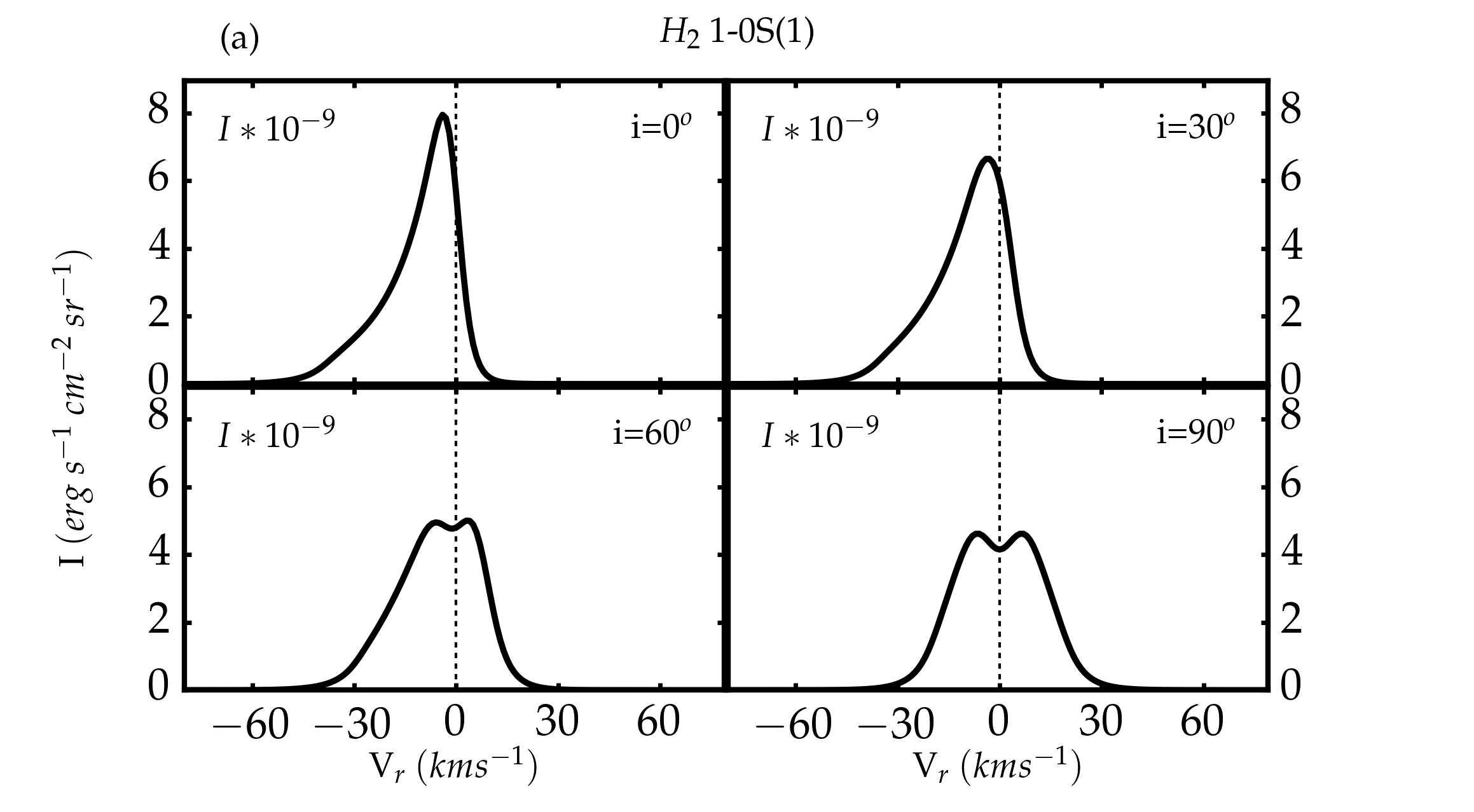
(a)

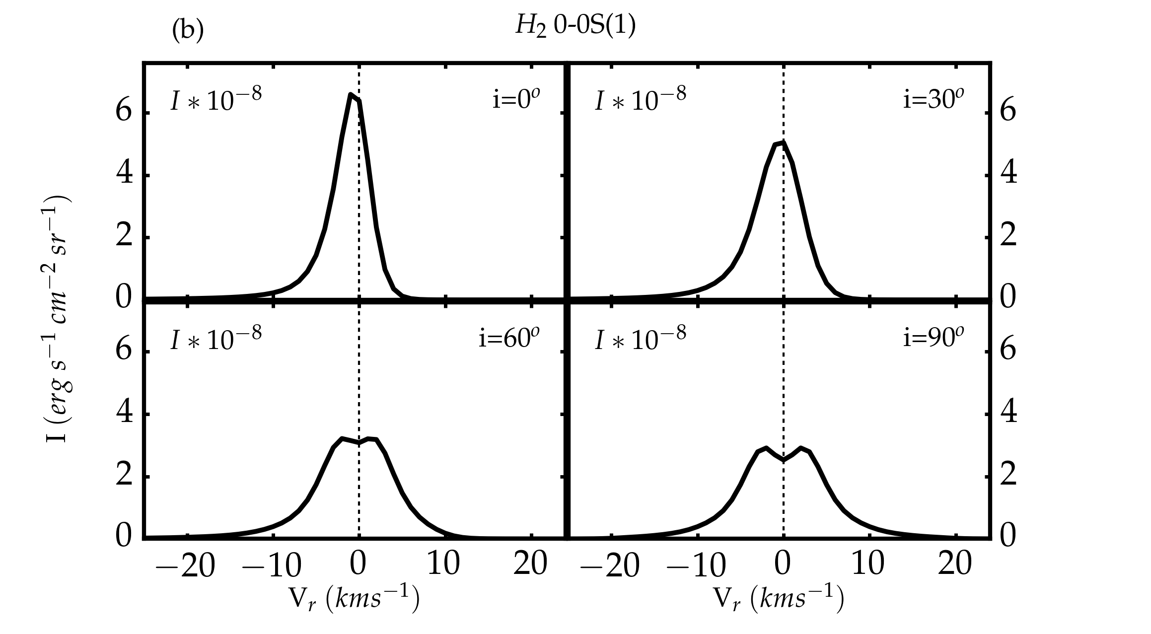
(b)

Figure 16: Line profiles of a whole bow shock parameterized by u₀ = 40 km s^-1, age = 10² years, b₀ = 1 and $\phi$ = 0^o. (a) for the H₂ 1-0S(1) line and (b) for the H₂ 0-0S(1) line. This figure shows the effect of the viewing angle on the line profile.

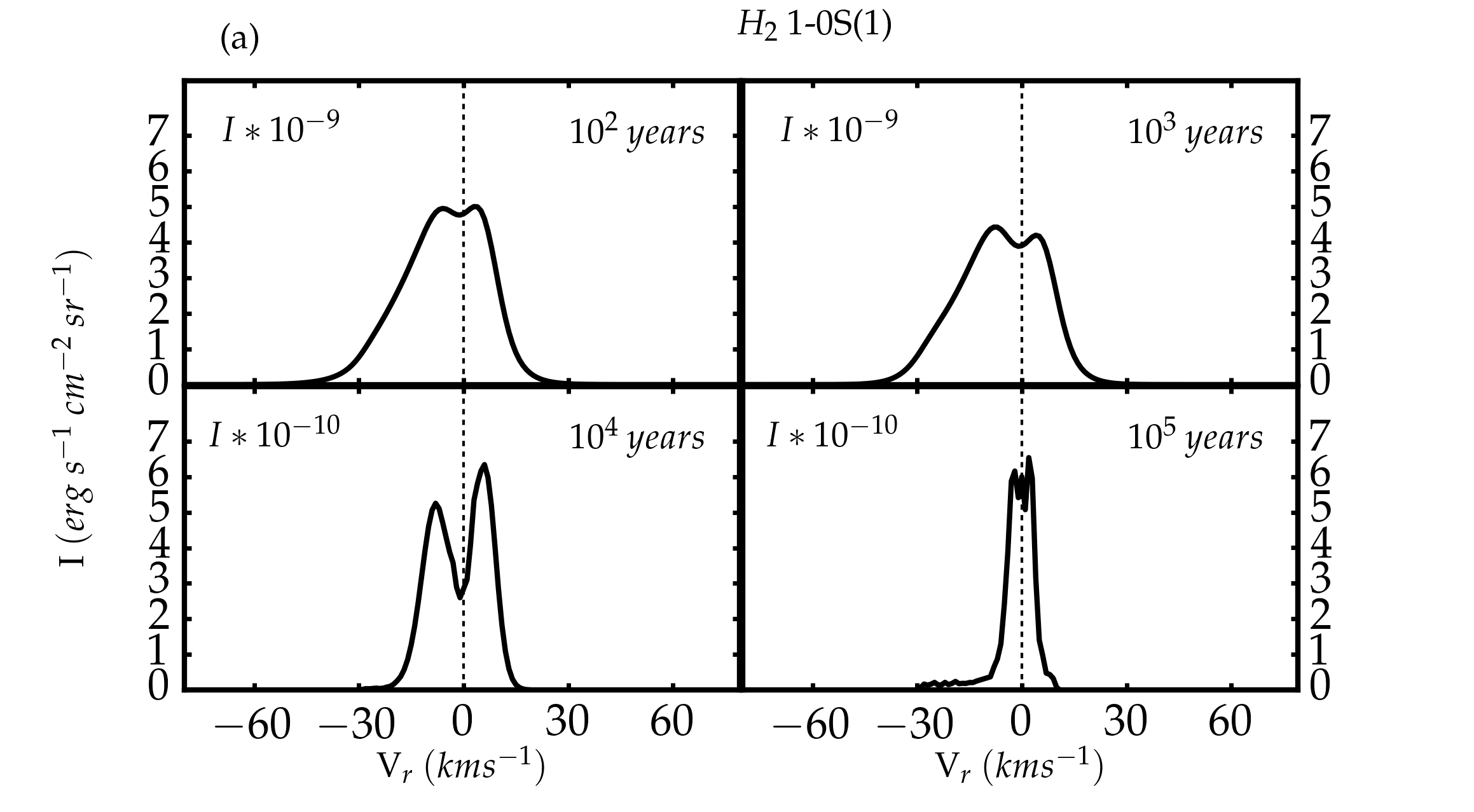
(a)

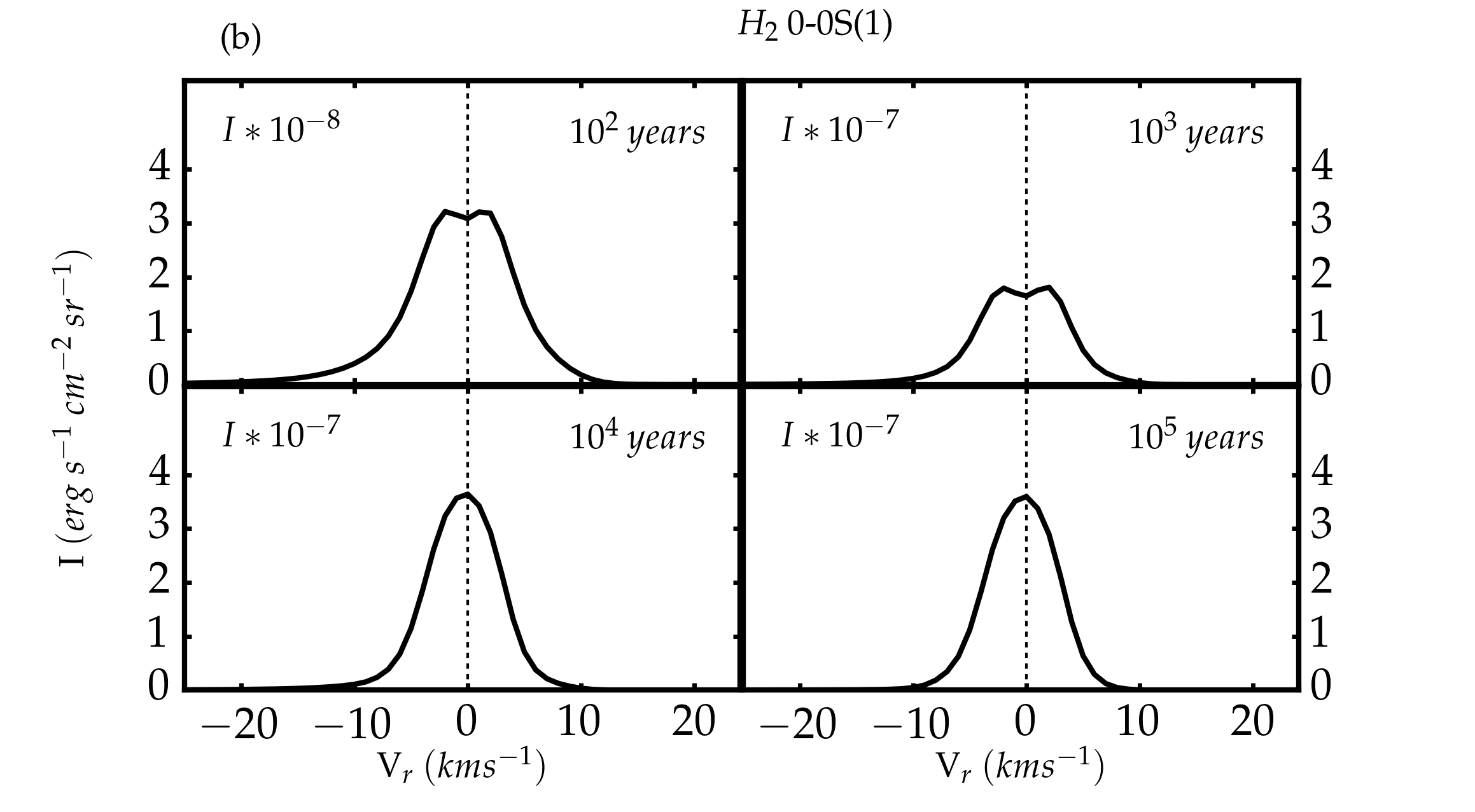
(b)

Figure 17: Line profiles of a whole bow shock parameterized by u₀ = 40 km s^-1, i = 60^o, b₀ = 1 and $\phi$ = 0^o. (a) for the H₂ 1-0S(1) line and (b) for the H₂ 0-0S(1) line. This figure shows the effect of the age on the line profile. Note the factor 10 change in flux scale between some panels

We assume the H₂ emission to be optically thin. Then the line profile is defined by integration over the whole volume of the bow shock, including the emission coming from each unit volume inside each planar shock composing the bow shock. The line emission at velocity V_r can be computed as follows :

$$f(V_{r},i)=\int_{u_{\bot}}P(u_{\bot}){\rm d}u_{\bot}\int_{\varphi}\frac{{\rm d}\varphi}{2\pi}\\ \int_{r}{\rm d}r\frac{R^{2}_{0}}{\sqrt{2\pi}\sigma_{T}(r,u_{\bot},b_{\parallel})}\epsilon(r,u_{\bot},b_{\parallel})e^{-\frac{[v_{\rm rad}(r,u_{\bot},b_{\parallel})-V_{r}]^{2}}{2\sigma^{2}_{T}(r,u_{\bot},b_{\parallel})}}$$ (11)

which includes Doppler broadening with $\sigma^{2}_{T}(r,\alpha)=k_{B}/m_{H_{2}}T_{H_{2}}(r,u_{\bot},b_{\parallel})$, the thermal velocity of the H₂ molecule. Note that the dependence on the azimuthal angle $\varphi$ occurs both in the expression of $b_{\parallel}$ (see equation 8) and the projection of $v_{\rm obs}$ onto the line-of-sight direction $\hat{\textbf{l}}$.

Figure 16a shows the effect of varying the viewing angle $i$ on the 1-0S(1) line shape. When the observer looks at the bow-shock from the point of view of the star ($i=0^{o}$), all the emission is blue-shifted, with a stronger emission at a slightly positive velocity, coming from the part of the shock structure closest to the star, close to the J-type front where this line is excited. As the viewing angle turns more to the flank ($i$ increases), the line of sight intercepts two sides of the working surface, one going away and the other going towards the observer. The line profile then becomes doubly peaked. We checked that the integrated line emission did not vary with the viewing angle $i$.

Figure 17a shows how the age affects the 1-0S(1) line profile at a given viewing angle of 60^o. As the shock becomes older, the J-tail entrance velocity decreases: this explains why the two peaks of the line profile get closer to each other as age proceeds. The velocity interval between the two peaks is proportional to the entrance velocity in the J-type tail of the shocks. Furthermore, as the entrance velocity decreases, the temperature inside the J-shock decreases accordingly and the Doppler broadening follows suit: the line gets narrower as time progresses. The width of the 1-0S(1) could thus serve as an age indicator, provided that the shock velocity is well known.

The 0-0S(1) line corresponds to a much lower energy level than the 1-0S(1) line: while the 1-0S(1) is sensitive to temperature and shines mostly around the J-type front, the 0-0S(1) line emits in the bulk of the shock, where gas is cooler. Since the 0-0S(1) line probes a colder medium, the resulting profiles are much narrower (figure 16b). For early ages (100 and 1000 yr), one can however still notice the double peak signature of the J-front (figure 17b). Because the temperature in the magnetic precursor is much colder than the transition’s upper level temperature of 1015 K for level (0,3). At these early ages, the 0-0S(1) line is shut off in the magnetic precursor (see figure 6, for example) and it therefore probes the J-shock part.

These results show that a wealth of dynamical information is contained in the line shapes. However, this information is hard to retrieve, as the line shaping process is quite convoluted. In particular, each line probes different regions of the shock depending on the upper level sensitivity to temperature. As an illustration, we plot the normalized line shapes for three different transitions in a 20 km s^-1 bow shock with pre-shock density 10⁴ cm^-3, age 1000 yr and $b_{0}=1$ (figure 19). This figure is meant to be compared with figure 2’s top panel in Santangelo et al. (2014), which plots resolved observations of H₂ lines in HH54. These observations come from two different slit positions: a CRIRES slit for 1-0S(1) and 0-0S(9) near the tip of the bow, orthogonal to the outflow axis, and a VISIR slit for the 0-0S(4) line along this axis. On the other hand, our models cover the whole extent of our bow shock, which questions the validity of the comparison. Despite this, some similarities are striking: the two lines 1-0S(1) and 0-0S(9) match perfectly and are blue-shifted. The insight from our computations allows us to link the good match between the line profiles of 1-0S(1) and 0-0S(9) to the very similar energy of the upper level of the two transitions. Furthermore, we checked in our models that the emission from the low energy 0-0S(4) is completely dominated by the C-type parts of our shocks, where the velocity is still close to the ambient medium velocity: this explains why this line peaks around $V_{r}=0$. This C-type component should shine all over the working surface of the bow shock, and the VISIR slit along the axis probably samples it adequately. Conversely, we checked that the emission coming from both lines 1-0S(1) and 0-0S(9) is completely dominated by the J-type parts of our shocks. Hence they should shine near the tip of the bow shock (traversed by the CRIRES slit) at a velocity close to that of the star and its observed radial speed should lie around $-u_{0}\cos(i)$, blue-shifted for an acute angle $i$.

Brand et al. (1989) managed to observe a few wide H₂ line profiles from OMC-1 Peak1 by using the UKIRT telescope, configured at a 5^′′ sky aperture and with a resolution of 12 km s^-1 full width at half maximum (FWHM). A single shock model was not able to reproduce these wide observed lines (as indicated by Rosenthal et al. 2000; Brand et al. 1989). A C-type bow shock model of Smith et al. (1991b) could reproduce these lines and widths, but this assumed a extremely high magnetic field strength of $\geq$ 50 mG (which amounts to b_∥ $\geq$ 50) while independent measurements in the same region gave much lower values: 3 mG by Zeeman splitting (Norris, 1984) or 10mG by polarisation (Chrysostomou et al., 1994). Here we use the best parameters listed in table 3 to try and reproduce the profile of the H₂ 1-0S(1) line with a more reasonable magnetisation. As mentionned in the previous subsection, the excitation diagram alone did not allow to constrain the terminal shock velocity. Now, the width of the profile allows us to constrain the velocity to about $u_{0}=100$ km s^-1 as illustrated by figure 19. The viewing angle $i\simeq$90^o can be adjusted to the position of the peak of the line profile. Note that shock models with $u_{\bot}>$40km s^-1 are not included in these line shape models. They should contribute little to the emission since H₂ molecules are dissociated at high shock velocities (both due to the high temperatures experienced in these shocks and to their radiative precursors).

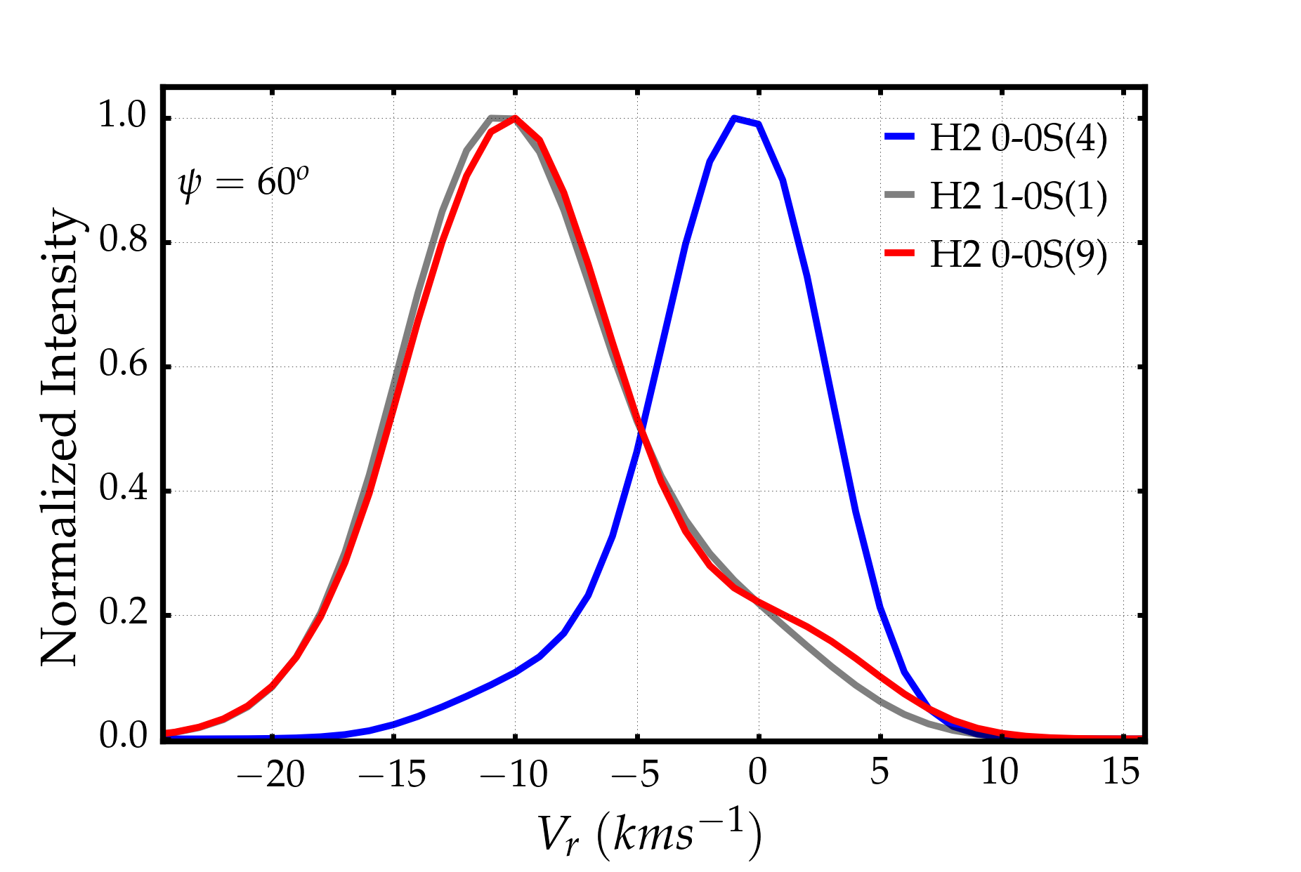
Figure 18: Line profiles of three different transitions in a bow shock at age 100 yr with parameters u₀=20 km s^-1, n_H=10⁴ cm^-3, b₀=1, and viewing angle i = 60^o.

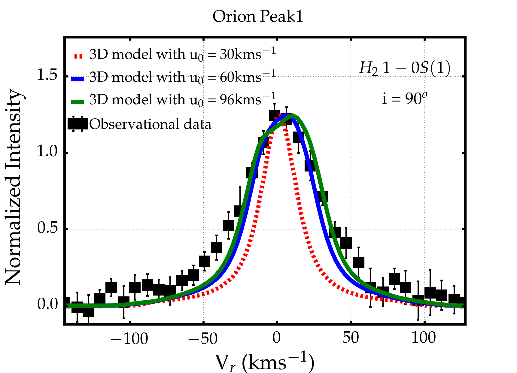
Figure 19: Comparison of the H₂ line profile between OMC-1 Peak1 observation and bow shock model. Black square: the observational data (Brand et al. 1989). Solid lines: our 3D model using parameters in table 3 with different values of u₀. The best 3D model constrains the terminal shock velocity to about 100 km s^-1.

5 Discussion and conclusion

In this study, we provide a mathematical formulation which arbitrarily links the shape of a bow shock to a distribution of planar shocks. Then, a simple convolution of this distribution with a grid of planar shocks allows to produce intensities and line shapes for any transition of the H₂ molecule.

We used that property to explain the dependence of the excitation diagram of a bow shock to its parameters: terminal velocity, density, shape, age, and magnetization properties (magnitude and orientation). The combination of a steeply decreasing distribution with a threshold effect linked to the energy of the upper level of each transition yields a “Gamow-peak” effect. A given H₂ level then reaches a saturation value when the terminal velocity is above a threshold which depends directly on the energy of the level. The magnetic field and the age dependence enter through the transition between the J-type and the C-type part of a time-dependent magnetized shock.

The wings of a bow shock usually have a larger surface than its nose. From this, it follows that the distribution and hence the global emission properties of a bow shock are generally dominated by low-velocity shocks. A direct consequence is that the excitation diagram of a whole bow shock resembles a 1D planar shock with a lower velocity: data interpretation with 1D models is likely to be biased towards low velocity. However, if the terminal velocity of the bow shock was estimated independently (from line Doppler broadening measurements, for example), we suggest that a magnetization adjustment from 1D models to the excitation diagram will over estimate the magnetization parameter. Previous authors (NY08, Neufeld et al., 2009) have suggested that the statistical equilibrium approximation could accurately reproduce observed intensities of low-energy pure rotational levels. We confirm this result, and its probable link to the distribution of entrance velocities as pointed out by NY08. However, we remark that this simple model does not satisfyingly reproduce the observations of the higher-lying transitions. A possible interpretation is that these levels are more sensitive to J-type shocks, where the sudden temperature jump is more likely to put the gas away from statistical equilibrium.

We provide some illustrations of how our results could improve the match between model and observations in BHR71 and Orion OMC-1. We show that 3D models largely improve the interpretation. In particular, we are able to obtain much better match than in previous works with relatively little effort (and with the addition of only one or two parameters compared to the 1D models: the magnetic field orientation and the shape of the bow shock).

We compute line shapes with an unprecedented care and examine their dependence to age and viewing angle. Although line shapes result from a convoluted process, they contain a wealth of dynamical information. In particular, we link the double peaked structure of 1-0S(1) in young bow shocks to the dynamics of their J-type part components. The line width results from the combined effects of geometry, terminal velocity, and thermal Doppler effect. We show how different lines probe different parts of the shocks depending on the temperature sensitivity of the excitation of their upper level. We show how our 3D model can reproduce the broad velocity profile of the H₂ 1-0S(1) line in Orion Peak1 with a magnetisation compatible with other measurements. The excitation diagram fails to recover dynamical information on the velocity (it only gives a minimum value), but the line shape width provides the missing constraint.

Further work will address some of the shortcomings of our method. First, it will be straightforward to apply similar techniques to the shocked stellar wind side of the bow shock working surface. Second, the different tangential velocities experienced on the outside and on the inner side of the working surface will very likely lead to turbulence and hence mixing, as multidimensional simulations of J-type bow shocks show. A challenge of the simplified models such as the ones presented here will be to include the mixing inside the working surface. All models presented here were run for a pre-shock ortho-para ratio of 3 : the dilute ISM is known to experience much lower ratios and we will explore the effect of this parameter on the excitation diagrams of bow-shocks in further work. Finally, our methods could be used to model other molecules of interest, provided that we know their excitation properties throughout the shock and that their emission remains optically thin. We expect that such developments will improve considerably the predictive and interpretative power of shock models in a number of astrophysical cases.

References

- Artymowicz & Clampin (1997) Artymowicz P., Clampin M., 1997, ApJ, 490, 863
- Benedettini et al. (2017) Benedettini M., et al., 2017, A&A, 598, A14
- Bourke (2001) Bourke T. L., 2001, ApJ, 554, L91
- Bourke et al. (1995) Bourke T. L., Hyland A. R., Robinson G., James S. D., Wright C. M., 1995, MNRAS, 276, 1067
- Bourke et al. (1997) Bourke T. L., et al., 1997, ApJ, 476, 781
- Brand et al. (1988) Brand P. W. J. L., Moorhouse A., Burton M. G., Geballe T. R., Bird M., Wade R., 1988, ApJ, 334, L103
- Brand et al. (1989) Brand P. W. J. L., Toner M. P., Geballe T. R., Webster A. S., 1989, MNRAS, 237, 1009
- Cesarsky et al. (1999) Cesarsky D., Cox P., Pineau des Forêts G., van Dishoeck E. F., Boulanger F., Wright C. M., 1999, A&A, 348, 945
- Chen et al. (2008) Chen X., Launhardt R., Bourke T. L., Henning T., Barnes P. J., 2008, ApJ, 683, 862
- Chièze et al. (1998) Chièze J.-P., Pineau des Forêts G., Flower D. R., 1998, MNRAS, 295, 672
- Chrysostomou et al. (1994) Chrysostomou A., Hough J. H., Burton M. G., Tamura M., 1994, MNRAS, 268, 325
- Corporon & Reipurth (1997) Corporon P., Reipurth B., 1997. p. 85
- DeWitt et al. (2014) DeWitt C., et al., 2014, European Planetary Science Congress 2014, EPSC Abstracts, Vol. 9, id. EPSC2014-612, 9, EPSC2014
- Draine (1978) Draine B. T., 1978, ApJS, 36, 595
- Draine & McKee (1993) Draine B. T., McKee C. F., 1993, ARA&A, 31, 373
- Flower & Pineau des Forêts (1999) Flower D. R., Pineau des Forêts G., 1999, in Ossenkopf V., Stutzki J., Winnewisser G., eds, The Physics and Chemistry of the Interstellar Medium.
- Flower & Pineau des Forêts (2003) Flower D. R., Pineau des Forêts G., 2003, MNRAS, 343, 390
- Flower & Pineau des Forêts (2015) Flower D. R., Pineau des Forêts G., 2015, A&A, 578, A63
- Flower et al. (2003) Flower D. R., Le Bourlot J., Pineau des Forêts G., Cabrit S., 2003, MNRAS, 341, 70
- Garay et al. (1998) Garay G., Köhnenkamp I., Bourke T. L., Rodríguez L. F., Lehtinen K. K., 1998, ApJ, 509, 768
- Giannini et al. (2004) Giannini T., McCoey C., Caratti o Garatti A., Nisini B., Lorenzetti D., Flower D. R., 2004, A&A, 419, 999
- Giannini et al. (2011) Giannini T., Nisini B., Neufeld D., Yuan Y., Antoniucci S., Gusdorf A., 2011, ApJ, 738, 80
- Gusdorf et al. (2011) Gusdorf A., Giannini T., Flower D. R., Parise B., Güsten R., Kristensen L. E., 2011, A&A, 532, A53
- Gusdorf et al. (2015) Gusdorf A., et al., 2015, A&A, 575, A98
- Gustafsson et al. (2010) Gustafsson M., Ravkilde T., Kristensen L. E., Cabrit S., Field D., Pineau Des Forêts G., 2010, A&A, 513, A5
- Hollenbach & McKee (1989) Hollenbach D., McKee C. F., 1989, ApJ, 342, 306
- Kaufman & Neufeld (1996) Kaufman M. J., Neufeld D. A., 1996, ApJ, 456, 611
- Kristensen et al. (2008) Kristensen L. E., Ravkilde T. L., Pineau Des Forêts G., Cabrit S., Field D., Gustafsson M., Diana S., Lemaire J.-L., 2008, A&A, 477, 203
- Le Bourlot et al. (2002) Le Bourlot J., Pineau des Forêts G., Flower D. R., Cabrit S., 2002, MNRAS, 332, 985
- Lesaffre et al. (2004a) Lesaffre P., Chièze J.-P., Cabrit S., Pineau des Forêts G., 2004a, A&A, 427, 147
- Lesaffre et al. (2004b) Lesaffre P., Chièze J.-P., Cabrit S., Pineau des Forêts G., 2004b, A&A, 427, 157
- Lesaffre et al. (2013) Lesaffre P., Pineau des Forêts G., Godard B., Guillard P., Boulanger F., Falgarone E., 2013, A&A, 550, A106
- Neufeld & Yuan (2008) Neufeld D. A., Yuan Y., 2008, ApJ, 678, 974
- Neufeld et al. (2009) Neufeld D. A., et al., 2009, ApJ, 706, 170
- Neufeld et al. (2014) Neufeld D. A., et al., 2014, ApJ, 781, 102
- Nisini et al. (2015) Nisini B., et al., 2015, ApJ, 801, 121
- Norris (1984) Norris R. P., 1984, MNRAS, 207, 127
- Ostriker et al. (2001) Ostriker E. C., Lee C.-F., Stone J. M., Mundy L. G., 2001, ApJ, 557, 443
- Parise et al. (2006) Parise B., Belloche A., Leurini S., Schilke P., Wyrowski F., Güsten R., 2006, A&A, 454, L79
- Raga et al. (2002) Raga A. C., de Gouveia Dal Pino E. M., Noriega-Crespo A., Mininni P. D., Velázquez P. F., 2002, A&A, 392, 267
- Rosenthal et al. (2000) Rosenthal D., Bertoldi F., Drapatz S., 2000, A&A, 356, 705
- Santangelo et al. (2014) Santangelo G., et al., 2014, A&A, 569, L8
- Shinn et al. (2011) Shinn J.-H., Koo B.-C., Seon K.-I., Lee H.-G., 2011, ApJ, 732, 124
- Smith (1992) Smith M. D., 1992, ApJ, 390, 447
- Smith & Brand (1990a) Smith M. D., Brand P. W. J. L., 1990a, MNRAS, 243, 498
- Smith & Brand (1990b) Smith M. D., Brand P. W. J. L., 1990b, MNRAS, 245, 108
- Smith et al. (1991a) Smith M. D., Brand P. W. J. L., Moorhouse A., 1991a, MNRAS, 248, 451
- Smith et al. (1991b) Smith M. D., Brand P. W. J. L., Moorhouse A., 1991b, MNRAS, 248, 730
- Suttner et al. (1997) Suttner G., Smith M. D., Yorke H. W., Zinnecker H., 1997, A&A, 318, 595
- White et al. (1986) White G. J., Richardson K. J., Avery L. W., Lesurf J. C. G., 1986, ApJ, 302, 701
- Wilkin (1996) Wilkin F. P., 1996, ApJ, 459, L31
- Yang et al. (2017) Yang Y.-L., Evans II N. J., Green J. D., Dunham M. M., Jørgensen J. K., 2017, ApJ, 835, 259