On Optimal Trees for Irregular Gather and Scatter Collectives

Abstract

We study the complexity of finding communication trees with the lowest possible completion time for rooted, irregular gather and scatter collective communication operations in fully connected, $k$-ported communication networks under a linear-time transmission cost model. Consecutively numbered processors specify data blocks of possibly different sizes to be collected at or distributed from some (given) root processor where they are stored in processor order. Data blocks can be combined into larger segments consisting of blocks from or to different processors, but individual blocks cannot be split. We distinguish between ordered and non-ordered communication trees depending on whether segments of blocks are maintained in processor order. We show that lowest completion time, ordered communication trees under one-ported communication can be found in polynomial time by giving simple, but costly dynamic programming algorithms. In contrast, we show that it is an NP-complete problem to construct cost-optimal, non-ordered communication trees. We have implemented the dynamic programming algorithms for homogeneous networks to evaluate the quality of different types of communication trees, in particular to analyze a recent, distributed, problem-adaptive tree construction algorithm. Model experiments show that this algorithm is close to the optimum for a selection of block size distributions. A concrete implementation for specially structured problems shows that optimal, non-binomial trees can possibly have even further practical advantage.

Keywords:

Gather and Scatter Collective Operations, Irregular Collective Operations, Communication trees, $k$-ported communication networks, Dynamic programming, NP-completeness.

1 Introduction

Collective gather and scatter operations play a role in many parallel applications for distributing or collecting data between a designated (root) process and other processes in the application. Gather and scatter operations are therefore included as collective operations in most interfaces and languages for parallel and distributed computing, notably in MPI [14], but for also in PGAS languages and frameworks like UPC++ [8, 21], and Global Arrays [15]. In these gather and scatter operations, a single process (thread) in a set of processes (threads) is to either collect data blocks from or distribute data blocks to all (other) processes (threads). While good algorithms for the regular variants of the problems where all data blocks have the same size are known for many types of communication networks under different communication models [1, 4, 11], this is much less the case for the irregular variants where different processes may contribute blocks of different sizes.

Collective communication operations, in particular irregular operations where processes contribute different amounts of data, pose two different algorithmic problems. The first is to determine for a(ny) given input data block distribution to the operation how fast the operation can be carried out, preferably by a closed-form expression. The second is to determine the complexity of building a communication schedule and structure that will allow to solve the problem in the determined time. For many regular operations, the latter problem can be solved in constant time per process, or with only a small, acceptable, say, logarithmic overhead, while yielding optimal completion time solutions. This is most often not the case for irregular operations.

For gather and scatter operations, trees are natural communication structures since data blocks flow to or from a single root process. This paper contributes to clarify the complexity of finding optimal (fastest, lowest completion time) communication trees for irregular gather and scatter problems under specific communication network assumptions that may serve as useful enough first approximations to real interconnects and communication systems. In particular we show that optimal trees can be constructed in polynomial time under certain natural constraints on how trees are built, whereas without these constraints, optimal tree construction is an NP-hard problem.

We study the problems under a linear transmission cost model, where the cost of transmitting a data block from one processor to another is proportional to the size of the block plus some constant start-up latency. Processors can only be involved in a single, or a small number of communication operations at a time. We assume that any processor can communicate with any other processor, but the cost of communication may be different for different pairs. Processes are bound one-to-one to processors, and ranked consecutively from $0$ to $p-1$, $p$ being the number of processors in the network. That is, our communication model is the fully connected, $k$-ported, non-homogeneous, linear cost communication network [9].

We distinguish between two types of communication trees. In the gather operation, data blocks from all processors are collected as a consecutive segment at the root processor in rank order. Conversely, for the scatter operation blocks stored in rank order at the root processor are distributed to the other processors such that processor $i$ eventually receives the $i$th block from the root. An ordered gather or scatter tree has the property that segments of data blocks at processors that are interior tree nodes are consecutive and in rank order, that is blocks for some processors $j,j+1,\ldots,j+s$ for $s\geq 0$ with $i\in[j,\ldots,j+s]$ for processor $i$. This has the advantage that processors that have to send blocks further on will never have to perform possibly costly, local reorderings of these blocks, and can make the implementation for, say, MPI, easier. However, this restriction may exclude communication schedules with lower completion times. For non-ordered trees, this constraint is dropped, and processors are allowed to send or receive not necessarily rank ordered segments of blocks in any order. Non-ordered trees may require reordering of blocks into rank order, at least at the root processor.

Concrete contributions of the paper are the following:

• For any given gather or scatter input instance, we show that with one-ported communication, optimal (fastest, lowest completion time), ordered communication trees can be found in polynomial time by a simple, dynamic programming algorithm running in $O(p^{3})$ operations for the homogeneous communication cost case, and in $O(p^{4})$ operations for the general, non-homogeneous case.

• We also show that optimal, binary communication trees can be computed by the same dynamic programming approach; all algorithms extend easily to the simpler, related problems of broadcast and reduction of data blocks (vectors).

• We use the offline, dynamic programming constructions to compare the completion times for different types of gather and scatter trees, in particular showing that a recently proposed, simple $\lceil\log p\rceil$ communication round, bottom up algorithm [20] can achieve good results compared to the optimal solutions.

• For specially structured problems consisting of two sizes of data blocks that are either large or small, we indicate that optimal, (non-)ordered trees can indeed perform (much) better on a concrete system than the adaptive binomial trees generated by the algorithm in [20].

• Finally, we show that computing optimal, non-ordered communication trees is an NP-complete problem, meaning that the problems of finding optimal ordered and non-ordered trees are computationally different.

1.1 Related work

Results on the gather and scatter collective communication operations can be found scattered over the literature. Standard, binomial tree and linear algorithms for the regular problems that are indeed used in most MPI library implementations, assuming a homogeneous, linear transmission cost model, or a simple hierarchical system are described in, e.g., [4, 12]. Extensions to multiple communication ports for some of these algorithms have been proposed in, e.g., [5, 16]. Algorithms for the regular scatter operation for the $LogP$ and $LogGP$ models were discussed in [1]. Other algorithms and implementations for the regular problems for MPI and UPC for a specific processor architecture can be found in [13]. Approaches to the irregular problems for MPI can be found in, e.g., [19, 7, 20], but it is fair to say that there has been overall little attention paid to these problems in the MPI community. More theoretical papers consider the problems in a different setting, e.g., that of finding optimal communication schedules for given trees [2].

2 The Model and the Problems

For now we leave concrete systems and interfaces like MPI aside but return to specific issues in later remarks. We define the communication models and problems in terms of processors carrying out communication operations. Since the gather and scatter operations are semantically “dual”, we mostly treat only one of them; the results translate into analogous results for the other.

2.1 Communication network model

We assume a fully connected network of $p$ communication processors ranked consecutively from $0$ to $p-1$ [9]. Processors can communicate pairwise in a synchronous, point-to-point fashion with one processor sending to another, receiving processor, both being involved during the transmission. Communication costs are linear but not necessarily homogeneous. More precisely, the time for transmitting a message of $m$ units (Bytes) from processor $i$ to processor $j$ is modeled as $\alpha_{ij}+\beta_{ij}m$ where $\alpha_{ij}$ is a start-up latency for the communication and $\beta_{ij}$ a time per transmitted unit. Furthermore, each processor will have a local copy cost of $\gamma_{i}m$ for copying a data block of $m$ units from one buffer to another. Communication is $k$-ported, $k\geq 1$, meaning that a communication processor can be engaged in at most $k$ communication operations at a time during which it is fully occupied. All $\lfloor p/2\rfloor$ processor pairs can communicate at the same time. The cost of a communication algorithm is the time for the slowest processor to complete communication and local copying under the assumption that all processors start at the same time.

Discussion

The communication network model captures certain features of modern high-performance systems, neglects others, and perhaps misrepresents some. It is useful, if it leads to algorithms that perform well on real systems (compared to other algorithms, designed under other assumptions), and if it serves to clarify inherent complexities in the gather and scatter problems.

The assumption that point-to-point communication is synchronous with both processors involved when communication takes place is common (albeit sometimes implicit) [3, 4], and leads to contention free algorithms for truly fully connected, one-ported networks. Since it fixes when communication takes place, it can make the analysis of collective algorithms significantly easier than in possibly more realistic models like $LogGP$ [1] that allow outstanding communication operations and overlap of both communication and computation. It often allows the development of optimal algorithms which is also significantly more difficult under $LogGP$, where few optimality results are known. Algorithms designed under the synchronous assumption often perform well in practice, where sometimes strict synchronous communication is relaxed for better performance. Models like $LogP$ and $LogGP$ can lead to algorithms with unrealistically large numbers of outstanding communication operations, unless some capacity constraint is externally imposed, and contention has to be accounted for. Ironically, the optimal scatter algorithm in the simple $LogP$ model has the root send data blocks to the other processors one after the other [1]. This does not correspond to practical experience [18, 20], and was one effect motivating the $LogGP$ model.

The non-homogeneous assumption makes it possible to model some aspects of systems where routing between some processors $i$ and $j$ is needed, or of clustered, hierarchical systems with different communication characteristics inside and between compute nodes. Sparse, non-fully connected networks can be captured by setting latency $\alpha_{ij}=\infty$ for processors $i$ and $j$ that are not connected in the network. The model cannot account for congestion in such networks, though. In such sparse networks, there may not be feasible solutions to the ordered gather and scatter problems. In order to guarantee feasible solutions in all cases, instead $\alpha_{ij}$ and $\beta_{ij}$ can be chosen to reflect the time for routing from processor $i$ to processor $j$. The model could be extended to piecewise linear transmission costs with different $\alpha_{ij}$ and $\beta_{ij}$ values for different message ranges.

With $k>1$ communication ports in the model adopted here, processors can be involved in up to $k$ concurrent communication operations at a time. Most of our results in the following will be for $k=1$. The general case with $k\geq 1$ is more difficult for reasons that will be pointed out. A number of results for regular collective communication operations in $k$-ported (torus) systems can be found in,e.g., [3, 5, 16].

The communication system is homogeneous if the communication costs for all processor pairs are characterized by the same start-up latency $\alpha$ and time per unit $\beta$. Likewise, homogeneous processors will have the same local copy cost $\gamma$. In our model, point-to-point communication is always out of or into consecutive communication buffers, which can necessitate local copies or reorderings of data blocks. In interfaces like MPI, this can sometimes be done implicitly by the use of derived datatypes [14, Chapter 4]. It is probably realistic to assume that a local copy can at least partially be performed concurrently with communication, and our results can be adopted to this. However, for simplicity we assume here that there is such a cost governed by $\gamma\geq 0$ that cannot be overlapped with communication. We tacitly assume that $\gamma_{i}\leq\beta_{ij}$ for any processors $i$ and $j$ in order to prevent artificial algorithms where some local data are sent back and forth between processors in order to save on local copy costs.

Albeit pairwise communication is synchronous, the overall execution of an algorithm is not. Each processor and communication port can engage in new communication as soon as it has completed its previous communication operation, independently of what the other processors are doing. This means that delays can be incurred when the communication partner is not yet ready. Optimal algorithms will minimize the overall effects of such delays. Note that under this asynchronous model, the information dissemination lower bound argument from round-based, synchronous models of $\lceil\log_{2}p\rceil$ communication rounds [3] does not apply. Optimal gather and scatter trees may well have a root degree smaller than $\lceil\log_{2}p\rceil$. Lemma 2 gives an example.

2.2 The irregular gather and scatter operations

The irregular gather/scatter operations are the following. Each processor has a local communication buffer of size $m_{i}$ units (Bytes). In addition, a designated root processor $r,0\leq r<p$ has a buffer of size $m=\sum_{i=0}^{p-1}m_{i}$ capable of storing data for all processors, including the root itself. We will refer to $m$ as the size of the gather/scatter problem. A gather or scatter problem is said to be regular, if all processors have the same buffer size $m_{i}=m/p$.

In the gather problem, each processor has a data block $[m_{i}]$ of size $m_{i}$ in its communication buffer, and the root has to collect all data blocks consecutively in rank order into a large segment of blocks $[m_{0},\-\ldots,\-m_{r-1},\-m_{r},\-m_{r+1},\-\ldots,\-m_{p-1}]$. The scatter problem is the opposite: The root has a large, consecutive segment of blocks in rank order $[m_{0},\-\ldots,\-m_{r-1},\-m_{r},\-m_{r+1},\-\ldots,\-m_{p-1}]$ in its buffer, and has to distribute the blocks to the processors such that processor $i$ eventually has the data block $[m_{i}]$ in its local buffer.

For both gather and scatter operations, the root processor $r$ has a data block $[m_{r}]$ to itself.

Discussion

In common interfaces like MPI and UPC, the root is always an externally given, fixed processor. Alternatively, the root could be decided by the algorithm solving the gather/scatter problem and lead to faster completion time. We consider both variations here. Concrete interfaces may give more control over the placement of data blocks at the root process. In MPI, for instance, the actual placement is controlled by an explicit offset for each block. The internal structure of blocks can likewise be controlled via MPI derived datatypes. Such features, however, do not change the essential algorithmic costs of the operations. The MPI gather/scatter operations also assume that the root process has a local block to itself which has to be copied from one buffer to another, unless the MPI_IN_PLACE option is supplied [14, Section 5.5]).

$$\mathrm{Time}(T^{r}_{\{r\}}) = 0$$

$$\mathrm{Time}(T^{r}_{R}(T^{r_{0}}_{R_{0}},T^{r_{1}}_{R_{1}},\ldots,T^{r_{j-1}}_{R_{j-1}},T^{r_{j}}_{R_{j}})) = \max(\mathrm{Time}(T^{r}_{R}(T^{r_{0}}_{R_{0}},T^{r_{1}}_{R_{1}},\ldots,T^{r_{j-1}}_{R_{j-1}})),\mathrm{Time}(T^{r_{j}}_{R_{j}}(\cdot)))+$$ (1)

$$\alpha_{r_{j}r}+\beta_{r_{j}r}\mathrm{Size}(T^{r_{j}}_{R_{j}})$$

$$\mathrm{Time}(T^{r}_{R}(T^{r_{0}}_{R_{0}},T^{r_{1}}_{R_{1}},\ldots,T^{r_{j-1}}_{R_{j-1}},T^{r}_{\{r\}})) = \mathrm{Time}(T^{r}_{R}(T^{r_{0}}_{R_{0}},T^{r_{1}}_{R_{1}},\ldots,T^{r_{j-1}}_{R_{j-1}}))+\gamma_{r}m_{r}$$ (2)

Figure 1: Equations defining the completion time of a gather or scatter tree $T^{r}_{R}$ over processors in $R$ rooted at processor $r\in R$ with (prefix of) subtrees $(T^{r_{0}}_{R_{0}},T^{r_{1}}_{R_{1}},\ldots,T^{r_{i}}_{\{r_{i}\}})$ in that order. One subtree must be $T^{r}_{\{r\}}$ for which the local copy at the root $r$ is done. $T^{r_{j}}_{R_{j}}(\cdot)$ denotes the $j$th subtree with its full sequence of subtrees.

2.3 Lower bounds

An obvious lower bound for both scatter and gather operations with root processor $r,0\leq r<p$ in a one-ported, homogeneous communication cost model is $\alpha+\beta(\sum_{i\neq r}m_{i})+\gamma m_{r}$ since all data blocks have to be sent from or received at the root from some (or several) processor(s), except for the root’s own block for which a local copy cost has to be paid. With non-homogeneous communication costs, a lower bound for, e.g., the scatter operation is $\min_{j\neq r}(\alpha_{rj}+\beta_{rj}\sum_{i\neq r}m_{i})+\gamma_{r}m_{r}$, determined by the fastest reachable neighbor processor of the root.

With instead $k>1$ communication ports that can work simultaneously, a lower bound for the homogeneous cost case becomes $\alpha+\beta(\lceil\sum_{i\neq r}m_{i}/k\rceil)+\gamma m_{r}$, assuming that data blocks $[m_{i}]$ can be arbitrarily split.

In the algorithms we consider here, this will be forbidden. Blocks can be compounded into larger segments of blocks, but individual blocks $[m_{i}]$ cannot be further subdivided. In this case, a lower bound is less trivial to formulate. Let $P_{0},P_{1},\ldots P_{k-1}$ be a partition of $\{0,\ldots p-1\}\setminus\{r\}$ into $k$ subsets. Assume that the data blocks are distributed over $k$ processors such that processor $i$ has the blocks in $P_{i}$. In that case, the gather and scatter operations can be completed in time $\alpha+\max_{0\leq j<k}\beta\sum_{i\in M_{j}}m_{i}+\gamma m_{r}$. A lower bound is given by a best such partition, e.g., by a partition that minimizes this gather/scatter time.

Discussion

For the $k$-ported lower bound, we assumed that the communication processor can with only one start-up latency $\alpha$ initiate or complete $k$ communication operations. This latency $\alpha$ may depend on $k$. It could instead be assumed that each initiated communication operation would occur its own start-up latency $\alpha$. See [3, 5, 16] for further discussion.

The lower bound for $k$-ported communication indicates that attaining it implicitly requires solving a possibly hard packing problem. Section 4 shows that this is the case even in the one-ported case, unless the allowed algorithms are further restricted.

2.4 Gather and scatter trees

The trivial algorithms for the gather and scatter operations let the root processor receive or send the data blocks from or to the other processors in some fixed order. The trivial algorithms have a high latency term of $(p-1)\alpha$. Possibly better algorithms let processors collect larger segments of data blocks that are later transmitted either as a whole or as smaller segments. We consider such algorithms here, but restrict attention to trees in the following strict sense.

Definition 1

Let the $p$ processors be organized in a tree rooted at root processor $r$. A gather tree algorithm allows each processor except $r$ to perform a single send operation (of a segment of blocks, towards the root). A scatter tree algorithm allows each processor except $r$ to perform a single receive operation (of a segment of blocks).

Discussion

The restriction to trees means that no individual blocks $[m_{i}]$ are allowed to be split, since this would imply that some processors in a gather tree perform several send operations. In the one-ported, homogeneous transmission cost model, this restriction is not serious, since communication time between two processors cannot be improved by pipelining, and pipelining a block through a longer path of processors cannot be faster than sending the block directly to the root. It also prevents algorithms that send some blocks several times, but this would be redundant anyway and cannot improve the gather completion time. All current implementations for the MPI gather and scatter operations are such tree algorithms (to the authors knowledge).

It is possible that a gather operation could be performed faster, especially with non-homogeneous communication costs by algorithms where processors collect segments of blocks that are then split into smaller segments and sent through different paths to the root (even without violating the restriction that individual blocks are not split). The author knows of no such DAG (Directed Acyclic Graph) algorithms for the gather and scatter operations.

It is well-known that optimal trees for regular gather and scatter problems in the linear transmission cost model are binomial trees with root degree $\lceil\log_{2}p\rceil$ when $\alpha>0$, see, e.g. [4]. As will be seen, this is not the case for the irregular problems.

2.5 Gather and scatter tree completion times

We now formally define the completion time (cost) of gather and scatter trees for the irregular operations. We (first) restrict the communication system to be one-ported.

Let $T^{r}_{R}$ be a gather/scatter tree spanning a set of processors $R$, rooted at processor $r\in R$. The size of $T_{R}$ is defined to be the sum of the sizes of the data blocks for the processors in the tree, $\mathrm{Size}(T^{r}_{R})=\sum_{i\in R}m_{i}$. Unless $T^{r}_{R}$ is a singleton tree $T^{r}_{\{r\}}$, the tree has some $j+1$ rooted subtrees as children, $T^{r_{0}}_{R_{0}},T^{r_{1}}_{R_{1}},\ldots,T^{r_{j}}_{R_{j}}$, for disjoint sets $R_{0},R_{1},\ldots,R_{k}$ with $r_{i}\in R_{i}$ that partition $R$. By $T^{r}_{R}(T^{r_{0}}_{R_{0}},T^{r_{1}}_{R_{1}},\ldots,T^{r_{j}}_{R_{j}})$ we denote the tree with (a prefix of) its subtrees in that order. Since the root by the one-ported communication assumption must communicate with these subtrees one after the other, the subtrees are considered in sequence, one after the other, and this order is given as part of the gather/scatter tree. Since local copying cannot by our assumptions be overlapped with communication, the root $r$ has at some point to perform its local copy of its data block $[m_{i}]$ which we account for by having one of the subtrees be the singleton $T^{r}_{\{r\}}$ for which it holds that $\mathrm{Size}(T^{r}_{\{r\}})=m_{r}$.

Definition 2

The completion time (cost), $\mathrm{Time}(T^{r}_{R}(T^{r_{0}}_{R_{0}},\-T^{r_{1}}_{R_{1}},\-\ldots,\-T^{r_{j}}_{R_{j}}))$, of a gather or scatter tree $T^{r}_{R}$ with a full sequence of subtrees $T^{r_{0}}_{R_{0}},T^{r_{1}}_{R_{1}},\ldots,T^{r_{j}}_{R_{j}}$ in that order under the one-ported network model is defined by the equations given in Figure 1. A tree $T^{r}_{R}$ is optimal if it has least completion time over all possible trees over $R$ with root $r$.

The equations in Figure 1 express that before processor $r$ can gather from its $i$th subtree $T^{r_{j}}_{R_{j}}$, it must have completed gathering from the previous subtrees. When also the gathering in $T^{r_{j}}_{R_{j}}$ by processor $r_{j}$ has been completed, the segment of data blocks from $T^{r_{j}}_{R_{j}}$ can be sent from processor $r_{j}$ to processor $r$ at the cost given by the (non-homogeneous) transmission cost model (Equation (1)). If the $j$th subtree is $r$ itself, the local copy has to be done (Equation (2)). For scattering, the root first sends the segment of data blocks for the $j$th subtree to processor $r_{j}$, and then scatter to the preceding subtrees. The completion time is the transmission time plus the time for the slower of the two concurrent scatter operations.

We note that given a gather or scatter tree as described, the completion time of the operation can be computed in $O(p)$ time steps by a bottom up traversal of the tree.

Figure 2: An ordered gather or scatter tree for $p=21$ processors rooted at processor $r=9$. The tree is neither binary nor binomial. In a gather operation, the root receives consecutive segments of data blocks from the subtrees from left to right. In a scatter operation, the root sends consecutive segments to the subtrees from right to left. Whether the tree is optimal depends on the data block sizes $m_{i}$.

In order to classify the complexity of constructing optimal gather and scatter trees we now introduce a further constraint on gather and scatter trees.

Definition 3

A gather or scatter communication tree $T^{r}_{R}$ is (strongly) ordered if $R=[i,i+1,\ldots,j]$ is a list of consecutively ranked processors from $i$ to $j,j\geq i$, $r\in R$, each subtree is likewise strongly ordered, and the subtrees are sequenced one after the other in such a way that the last processor in any subtree is the processor ranked immediately before the first processor in the immediately following subtree.

A gather or scatter tree $T^{r}_{R}$ that is not strongly ordered non-ordered.

Discussion

Ordered versus non-ordered are structural properties of the communication trees. The completion time of Definition 2 assumes $k=1$ communication ports, but can be extended also to $k>1$ communication ports. Each port can independently receive or send blocks from a subset of the subtrees, one after the other, and the completion time would be the time for the last port to finish. Subtrees could be assigned to ports statically. Alternatively, it could be assumed that the assignment is done greedily, such that a finished ports starts sending or receiving from the next subtree in the sequence not assigned to a port. Note that the precise choice would not change the cost of an optimal completion time tree.

An ordered communication tree with four (ordered) subtrees is shown in Figure 2. In an ordered gather tree algorithm, each processor gathers and maintains only a consecutively ordered segment of data blocks from its children, and at no stage will blocks have to be permuted to fulfill the consecutive ordering constraint at the root. Also no prior offset calculations are needed, the next block segment can be placed in the communication buffer immediately after the already received blocks. If the ordered subtrees are not sequenced one after another as defined, and the block segments are received in some possibly non-consecutive order (as could be the case in a non-blocking, asynchronous communication model), the tree is still said to be weakly ordered. Note that a gather tree is strongly ordered if and only if the strongly ordered subtrees are sequenced such that the roots are in increasing rank order.

Non-ordered trees provide more freedom to reduce completion time, but permutation of blocks at the root or other non-leaf processors to put blocks into rank order could lead to extra costs of $\gamma_{r}m$ or more. Still note that an optimal, non-ordered tree may complete faster than an optimal, weakly ordered tree, which may in turn complete faster than an optimal, ordered tree.

In [20] it was shown that ordered, binomial gather and scatter trees for the homogeneous transmission cost model can be found efficiently in a distributed manner with a root processor chosen by the algorithm. We use this result here, and also compare these trees against other (optimal) trees in our cost model in Section 5. These trees are good, but (usually) not optimal; but (as will be seen) better trees require a large effort to construct.

Proposition 1

Let $m_{i},i=0,\ldots,p-1$ be the data block sizes for the $p$ processors. With homogeneous communication costs, and local copy cost $\gamma=\beta$, strongly ordered gather and scatter trees with completion time $\lceil\log_{2}p\rceil\alpha+\beta\sum_{i=0}^{p-1}m_{i}$ exist, and can be constructed offline in $O(p)$ steps.

The trick of the construction is to pair adjacent, ordered subtrees with the same number of processors, but such that the subtree with the smaller amount of data sends (in the gather case) its data to the tree with the larger amount of data.

3 Polynomial Time Constructions for Ordered Trees

Figure 3: Structure of optimal completion time, non-ordered and ordered, gather and scatter trees. The communication time (for gather, in the direction of the root $r$) is $\alpha_{r^{\prime}r}+\-\beta_{r^{\prime}r}\mathrm{Size}(T^{r^{\prime}}_{\bar{R}})$, and $\alpha_{r^{\prime}r}+\-\beta_{r^{\prime}r}\mathrm{Size}(T^{r^{\prime}}_{[k+1,\ldots,p-1]})$ or $\alpha_{r^{\prime}r}+\-\beta_{r^{\prime}r}\mathrm{Size}(T^{r^{\prime}}_{[0,\ldots,k,]})$, respectively, which has to be paid in addition to the respective times $\max(\mathrm{Time}(T_{R}),\mathrm{Time}(T_{\bar{R}}))$ and $\max(\mathrm{Time}(T_{[0,\ldots,k]}),\mathrm{Time}(T_{[k+1,\ldots,p-1]}))$ for completing the subtrees. For the ordered trees, the cases where $r\in[0,\ldots,k]$ and $r\in[k+1,\ldots,p-1]$ both have to be considered.

$$\mathrm{Time}(T^{r}_{[r]}) = 0$$

$$\mathrm{Time}(T^{r}_{[i,\ldots,j]}) = \max(\mathrm{Time}(T^{r}_{[i,\ldots,k]}),\mathrm{Time}(T^{r^{\prime}}_{[k+1,\ldots,j]}))+\alpha_{r^{\prime}r}+\beta_{r^{\prime}r}\mathrm{Size}(T^{r^{\prime}}_{[k+1,\ldots,j]})$$ (3)

$$\mathrm{Time}(T^{r}_{[i,\ldots,j]}) = \max(\mathrm{Time}(T^{r^{\prime}}_{[i,\ldots,k]}),\mathrm{Time}(T^{r}_{[k+1,\ldots,j]}))+\alpha_{r^{\prime}r}+\beta_{r^{\prime}r}\mathrm{Size}(T^{r^{\prime}}_{[i,\ldots,k]})$$ (4)

$$\mathrm{Time}(T^{r}_{[r,\ldots,j]}) = \max(\gamma_{r}m_{r},\mathrm{Time}(T^{r^{\prime}}_{[r+1,\ldots,j]}))+\alpha_{r^{\prime}r}+\beta_{r^{\prime}r}\mathrm{Size}(T^{r^{\prime}}_{[r+1,\ldots,j]})$$ (5)

$$\mathrm{Time}(T^{r}_{[i,\ldots,r]}) = \mathrm{Time}(T^{r^{\prime}}_{[i,\ldots,r-1]})+\alpha_{r^{\prime}r}+\beta_{r^{\prime}r}\mathrm{Size}(T^{r^{\prime}}_{[i,\ldots,r-1]})+\gamma_{r}m_{r}$$ (6)

Figure 4: Equations characterizing the completion time of ordered gather and scatter trees over a range of processors $[i,\ldots,j]$ rooted at processor $r\in[i,\ldots,j]$.

We now show that optimal, smallest completion time, ordered gather and scatter trees can be constructed in polynomial trees.

3.1 Characterizing tree completion times

The following observation express the tree completion times more concisely and is crucial for all following algorithms and results. Propositions 2 and 3 both assume one-ported communication, and are difficult to extend to more communication ports.

Proposition 2

An optimal completion time, non-ordered communication tree for an irregular gather (or scatter) operation over a set $P$ (of at least two) one-ported processors consists in a subtree $T^{r}_{R}$ rooted at some processor $r\in R$ and a subtree $T^{r^{\prime}}_{\bar{R}}$ rooted at some other processor $r^{\prime}\in\bar{R}$ where $R$ and $\bar{R}$ is a partition of $P$ with communication between processors $r$ and $r^{\prime}$ that minimizes $\mathrm{Time}(T^{r}_{P})$ defined by the following equations.

$$\mathrm{Time}(T^{r}_{\{r\}}) = 0$$

$$\mathrm{Time}(T^{r}_{P}) = \max(\mathrm{Time}(T^{r}_{R}),\mathrm{Time}(T^{r^{\prime}}_{\bar{R}}))+\alpha_{r^{\prime}r}+\beta_{r^{\prime}r}\mathrm{Size}(T^{r^{\prime}}_{\bar{R}})$$ (7)

$$\underset{R=\{r\}}{\mathrm{Time}(T^{r}_{P})} = \max(\gamma_{r}m_{r},\mathrm{Time}(T^{r^{\prime}}_{\bar{R}}))+\alpha_{r^{\prime}r}+\beta_{r^{\prime}r}\mathrm{Size}(T^{r^{\prime}}_{\bar{R}})$$ (8)

Proof: The partition of $P$ into $R$ and $\bar{R}$ in Equation (7) defines the last subtree in the sequence of subtrees of $T^{r}_{R}$ as in Equation (1) of Definition 2, and assigns the same cost. Equation (8) defines the place in the sequence of subtrees of $r$ for performing the local copy by partitioning $P$ into $R=\{r\}$ and $\bar{R}=R\setminus\{r\}$ and corresponds to Equation (2). This always puts the subtrees over $\bar{R}$ after the local copy in the sequence, such that completion of $T^{r^{\prime}}_{\bar{R}}$ can be done concurrently with the local copy of cost $\gamma_{r}m_{r}$. An optimal, non-ordered tree must have this structure, since the case where communication is done first and then the local copy (which cannot be overlapped) would have cost $\mathrm{Time}(T^{r^{\prime}}_{\bar{R}})+\alpha_{r^{\prime}r}+\beta_{r^{\prime}r}\mathrm{Size}(T^{r^{\prime}}_{\bar{R}})+\gamma_{r}m_{r}$ which is larger than $\max(\gamma_{r}m_{r},\mathrm{Time}(T^{r^{\prime}}_{\bar{R}}))+\alpha_{r^{\prime}r}+\beta_{r^{\prime}r}\mathrm{Size}(T^{r^{\prime}}_{\bar{R}})$. A tree that is optimal according to the proposition will therefore also be optimal according to Definition 2, and conversely. $\Box$

The importance of Proposition 2 is in characterizing optimal completion time trees.

Corollary 1

In the one-ported transmission cost model, optimal completion time gather and scatter trees exhibit optimal substructure.

Proof: In order for the completion time of Equation (7) to be optimal, both subtrees $T^{r}_{R}$ and $T^{r^{\prime}}_{\bar{R}}$ must be optimal; if not a possibly better completion time tree could be found. $\Box$

Ordered and non-ordered trees are shown in Figure 3 to illustrate Proposition 2 and the following Proposition 3.

Corollary 1 states that the problem of constructing optimal gather and scatter trees can be solved by dynamic programming. Unfortunately, Proposition 2 seems to imply that all possible partitions of the set of processors into the subsets $R$ and $\bar{R}$ need to be considered, and for non-ordered trees, this might indeed be so as Section 4 shows. For (strongly) ordered trees where $P=[i,i+1,\ldots,j]$ is a consecutive list of processors, however, only $j-i$ partitions have to be considered, namely $R=[i,\ldots,k]$ and $\bar{R}=[k+1,\ldots,j]$ for $k=i,\ldots,j-1$.

Proposition 3

An optimal, least cost, ordered communication tree for an irregular gather or scatter problem over a list of processors $P=[i,i+1,\ldots,j]$ with at least two processors consists in ordered subtrees over $[i,\ldots,k]$ and $[k+1,\ldots,j]$ for some $k,i\leq k<j$ with roots $r\in[i,\ldots,k]$ and $r^{\prime}\in[k+1,\ldots,j]$, or $r\in[k+1,\ldots,j]$ and $r^{\prime}\in[i,\ldots,k]$ that minimizes $\mathrm{Time}(T^{r}_{P})$ defined by the equations given in Figure 4.

Proof: The proposition follows by specialization of Proposition 2, keeping track of whether the root is in the list of processors $[i,\ldots,k]$ or $[k+1,\ldots,j]$. Equations (3) and (4) correspond to Equation (7). Equations (5) and (6) correspond to Equation (8) but are asymmetric because of the strong ordering constraints. When $r\in[r,\ldots,j]$ is the first processor, the local copy can be done concurrently with completing the tree $T^{r^{\prime}}_{[r+1,\ldots,j]}$ after which communication is paid for. When on the other hand $r\in[i,\ldots,r]$ is the last processor, the data blocks $[m_{i},\ldots,m_{r-1}]$ must be communicated first after which the local copy can take place. $\Box$

$$C[i,i,i] = 0$$

$$\underset{i<j}{C[i,j,r]} = \left\{\begin{array}[]{cl}\min_{i+1\leq r^{\prime}<j}[\max(\gamma_{r}m_{r},C[i+1,j,r^{\prime}])+\mathrm{comm}_{r^{\prime}r}(S[i+1,j])]&r=i\\ \min_{i\leq k<j}\min_{k+1\leq r^{\prime}\leq j}[\max(C[i,k,r],C[k+1,j,r^{\prime}])+\mathrm{comm}_{r^{\prime}r}(S[k+1,j])]&r\in[i+1,\ldots,k]\\ \min_{i\leq k<j}\min_{i\leq r^{\prime}\leq k}[\max(C[i,k,r^{\prime}],C[k+1,j,r])+\mathrm{comm}_{r^{\prime}r}(S[i,k])]&r\in[k+1,\ldots,j-1]\\ \min_{i\leq r^{\prime}<j-1}[C[i,j-1,r^{\prime}]+\mathrm{comm}_{r^{\prime}r}(S[i,j-1])+\gamma_{j}m_{j}]&r=j\\ \end{array}\right.$$

Figure 5: Dynamic programming equations for constructing optimal, ordered gather under a non-homogeneous communication cost model $\mathrm{comm}_{ij}(m)=\alpha_{ij}+\beta_{ij}m$ where communication is from a non-root processor $r$ to root processor $r$. For the scatter tree, communication cost from root processor $r$ to non-root $r^{\prime}$ is incurred instead.

Discussion

Proposition 2 and Corollary 1 do not seem to extend to the case with $k>1$ communication ports. An optimal completion time $k$-ported tree is not described by partitioning $P$ into $k+1$ optimal subtrees where $k$ ports of the root in one subtree gathers or scatters from or to $k$ other subtrees. The $k$ subtrees must all have completed (as determined by the slowest port of the root processors in these trees) before communication and be optimal, but the one tree with the root does not have to be optimal. A slow port at the root could communicate with a fast subtree, leading to an overall faster completion time. Constructing optimal trees for the $k>1$ ported case seems more difficult than with only one port, and it is not known (to the author) whether this problem can be solved as efficiently.

3.2 Dynamic programming algorithms

Proposition 3 and Corollary 1 show that the problem of finding optimal, ordered gather and scatter trees for the one-ported communication model can be solved efficiently by dynamic programming by building up optimal subtrees for larger and larger ranges of processors $[i,\ldots,j]$. Using the optimality criteria from Proposition 3, we now develop the dynamic programming equations for both non-homogeneous and homogeneous communication costs.

The size of a tree $T^{r}_{[i,j]}$ over a range of processors $[i,\ldots,j]$ can be computed in constant time as $\mathrm{Size}(T^{r}_{[i,\ldots,j]})=S[j]-S[i-1]$ from precomputed prefix sums $S[i]=\sum_{j=0}^{i}m_{j}$ (with $S[-1]=0$). The completion time of an ordered tree over a range of processors $[i,\ldots,j]$ is determined by the completion times of smaller, optimal subtrees over ranges $[i,\ldots,k]$ and $[k+1,\ldots,j]$ and the communication time for transmitting between the subtrees. With non-homogeneous communication costs, transmission times can be different between different pairs of processors. We let $C[i,j,r]$ denote the completion time of an optimal gather or scatter tree over processors in the range $[i,\ldots,j]$ rooted at processor $r\in[i,\ldots,j]$, and $\mathrm{comm}_{ij}(m)=\alpha_{ij}+\beta_{ij}m$ the cost of communicating a block of size $m$ in the non-homogeneous transmission cost model, with in addition $\mathrm{comm}_{ij}(0)=0$ meaning no communication when no data. Now, $C[i,j,r]$ can be computed as given by the equations in Figure 5 which follow directly from Proposition 3, given that the required values $C[i,k,r]$ and $C[k+1,j,r^{\prime}]$ are available. There is no cost for singleton trees $C[i,i,i]$. If the root $r$ is the first processor $i$, there is a local copy cost, concurrently with which the other tree over processors $[i+1,\ldots,j]$ can be completed, with the additional cost of the communication between processor $i$ and the root $r^{\prime}$ in the best tree over the processors $[i+1,\ldots,j]$. Similarly if the root $r$ is the last processor $j$ in the range, with the difference that the local copy in this case can be done only after the communication has taken place. Otherwise, there are two cases, depending on whether $r\in[i,\ldots,k]$ or $r\in[k+1,\ldots,j]$. In both, the larger of the completion times for the best two subtrees have to be paid, in addition to communication costs between the root processors $r$ and $r^{\prime}$. The cost of an optimal gather or scatter tree over the whole range of processors $[0,p-1]$ with root $r$ is given by the table entry $C[0,p-1,r]$. If the overall best tree with root processor $r$ chosen by the algorithm is needed, this is given by $\min_{0\leq r<p}C[0,p-1,r]$.

The values $C[i,j,r]$ can be maintained in a three-dimensional table $C$ that can be computed bottom up, step by step increasing the size of the processor ranges $[i,\ldots,j]$. Each such step requires a pass over all $i$, all $k,i\leq k<j$, and all $r^{\prime}\in[i,\ldots,j]$, for a total of $O(p^{4})$ operations over all range increasing steps. Computing the sizes $S[i,j]$ is done on the fly in constant time from the precomputed prefix sums. The actual trees can be constructed by keeping an additional two-dimensional table $\mathrm{root}[i,j]$ that keeps track of the subtree root $r^{\prime}$ chosen for the processor range $[i,\ldots,j]$. The trees constructed are not necessarily binomial, or binary; each subtree may have an arbitrary degree between $0$ and $p-1$. We say that optimal trees have variable degree, and have argued for the following theorem.

Theorem 1

Completion time optimal, variable degree gather and scatter trees for the irregular gather and scatter problems on $p$ fully connected, one-ported processors under a linear-time, non-homogeneous transmission cost model can be computed in $O(p^{4})$ operations using $O(p^{3})$ space.

Proof: Optimality follows from Proposition 3, and the complexity from the dynamic programming construction of the three-dimensional table $C$. Each part of the equations in Figure 5 takes at most $O(p^{2})$ time, and the table can be constructed by two nested loops of at most $p$ iterations each. $\Box$

$$C[i,i] = 0$$

$$C[i,i+1] = \min\left\{\begin{array}[]{l}\max(\gamma m_{i},C[i+1,i+1])+\mathrm{comm}(S[i+1,i+1])\\ C[i,i]+\mathrm{comm}(S[i,i])+\gamma m_{j}\\ \end{array}\right\}$$

$$\underset{i+1<j}{C[i,j]} = \min_{i\leq k<j}[\max(C[i,k],C[k+1,j])+\min(\mathrm{comm}(S[i,k]),\mathrm{comm}(S[k+1,j]))]$$

Figure 6: Dynamic programming equations for constructing optimal, ordered gather and scatter trees under a homogeneous communication cost model $\mathrm{comm}(m)=\alpha+\beta m$.

For non-homogeneous communication systems, when two subtrees over a range of processors communicate, it is necessary to consider all possible best rooted trees over the range, since the communication cost from the different roots may differ. For homogeneous systems, where the $\alpha$ and $\beta$ parameters are the same for all pairs of processors, this is not the case, and it suffices to keep track of the overall best rooted tree for each processor range $[i,\ldots,j]$ instead of each possible root in $[i,\ldots,j]$. This leads to the simplified, dynamic programming equations given in Figure 6 which find a least cost gather or scatter tree for a best possible root. Since only a best possible root needs to be maintained for each range, this lowers the overall complexity by a factor of $p$ to $O(p^{3})$ operations, leading to the following theorem.

Theorem 2

Completion optimal variable degree gather and scatter trees for the irregular gather and scatter problems on $p$ fully connected, one-ported processors under a linear-time, homogeneous transmission cost model can be computed in $O(p^{3})$ operations using $O(p^{2})$ space.

Proof: The correctness of the equations in Figure 6 follow from Proposition 3. The two-dimensional $C$ table is constructed by a standard, dynamic programming algorithm in $O(p^{3})$ operations. $\Box$

We note that by explicitly keeping track of the root chosen for each range $[i,\ldots,j]$ in a separate, two-dimensional table $\mathrm{root}[i,j]$, the computed trees can easily be reconstructed as is a standard dynamic programming technique, see, e.g., [6]. For computing a tree rooted at an externally given root $r$, the equations have to be modified so that communication is always with this root for processor ranges $[i,\ldots,j]$ with $r\in[i,\ldots,j]$. Also this is straightforward.

$$C[i,i] = 0$$

$$\underset{i<j}{C[i,j]} = \min\left\{\begin{array}[]{l}\min_{i<k<j}\left[\max(\max(\gamma m_{i},C[i+1,k])+\mathrm{comm}(S[i+1,k]),C[k+1,j])+\mathrm{comm}(S[k+1,j])\right]\\ \min_{i<k<j}\left[\max(C[i,k-1]+\mathrm{comm}(S[i,k-1])+\gamma m_{k},C[k+1,j])+\mathrm{comm}(S[k+1,j])\right]\\ \min_{i\leq k<j-1}\left[\max(C[i,k]+\mathrm{comm}(S[i,k]),C[k+1,j-1])+\mathrm{comm}(S[k+1,j-1])+\gamma m_{j}\right]\\ \max(\gamma m_{i},C[i+1,j])+\mathrm{comm}(S[i+1,j])\\ C[i,j-1]+\mathrm{comm}(S[i,j-1])+\gamma m_{i}\\ \end{array}\right\}$$

Figure 7: Dynamic programming equations for constructing cost optimal, ordered binary trees under a homogeneous transmission cost model $\mathrm{comm}(m)=\alpha+\beta m$.

3.3 Dynamic programming for other trees

Binary (or other fixed-degree trees) are sometimes used for implementing rooted collective operations like broadcast and reduction. Dynamic programming can likewise be used to compute optimal binary trees for these problems. For completeness (and because this could be relevant for, e.g., sparse reduction problems, or for exploring the structure of optimal trees) we state the corresponding dynamic programming equations. There are five cases to consider. The root of an ordered, binary tree is either “at the left”, “at the right” or somewhere “in the middle”, or the root has only one child, either left or right. The equations assuming a homogeneous cost model are given in Figure 7. Also here, a best possible root is chosen by the algorithm; it is easy to modify to the case where the root is externally given; here only the last extension step filling in table entry $C[0,p-1]$ needs to be adapted to sending to the fixed root $r$ and choose the best subtrees out of the five possible cases. This gives the following theorem.

Theorem 3

Completion time optimal binary gather and scatter trees for the irregular gather and scatter problems on $p$ fully connected, one-ported processors under a linear-time, homogeneous transmission cost model can be computed in $O(p^{3})$ operations ($O(p^{4})$ for non-homogeneous communication costs) and $O(p^{2})$ space ($O(p^{3})$ for non-homogeneous communication costs).

By the same techniques, optimal, ordered trees for broadcast and reduction can likewise be computed. The only difference is that the size for each node in such trees are the same, namely $S[i,j]=m$ for all $i\leq j$. Note that the trees computed in this way are special in the sense that the subtrees of interior nodes span consecutive ranges of processors $[i,\ldots,j]$. As Section 4 will show, not all optimal broadcast trees have this structure. However, this property is useful for reduction operations, where binary reduction operations may have to be performed in processor rank order (unless the operation is commutative); MPI for instance has such constraints.

Theorem 4

Cost-optimal, ordered broadcast and reduction trees on $p$ fully connected, one-ported processors under a linear-time, non-homogeneous transmission cost model can be computed in $O(p^{4})$ operations and $O(p^{3})$ space (respectively $O(p^{3})$ time and $O(p^{2})$ space under homogeneous costs).

Discussion

The dynamic programming algorithms are hardly practically relevant, unless trees can be precomputed and reused many times in persistent communications, or unless problems are so large that $m$ is $\Omega(p^{4})$ (or $\Omega(p^{3})$) and actual communication time offsets the tree construction time. Furthermore, the constructions are offline, and require full knowledge of the block sizes for all processors. In MPI and other interfaces, only the root processor has this information. A schedule could be computed at the root, and sent to the other processors (with at least a linear time communication overhead), an idea that was attempted in [19].

4 Hardness of the Non-Ordered Constructions

The ordering constraint on communication trees made polynomial time constructions of optimal gather and scatter trees possible. The following theorems show that finding cost-optimal trees when subtrees are not required to be ordered is a different, harder problem. The first and second are easy observations.

Theorem 5

Constructing optimal, minimum completion time broadcast trees in the non-homogeneous, fully-connected, one-ported, linear transmission cost model is NP-hard.

This is a simple observation and reduction from the Minimum Broadcast Time problem, see [10, ND49] and [17]. The Minimum Broadcast Time problem is, for a given unweighted, undirected graph $G$ and root vertex $u$ to find the minimum number of communication rounds required to broadcast a unit size message from $u$ to all other vertices in $G$, where in each communication round, a vertex can send a message to some other vertex along an edge of $G$. We take $\alpha_{uv}=1$ for all edges $uv$ of $G$, and $\alpha_{u^{\prime}v^{\prime}}=\infty$ for edges $u^{\prime}v^{\prime}$ not in $G$, $m=1$ and all $\beta_{uv}=1$. An optimal broadcast tree in the non-homogeneous cost model would be a solution to the Minimum Broadcast Time problem, and vice versa.

As indicated in Section 2.3 with $k$-ported communication, $k>1$, an optimal algorithm would entail solving a hard packing problem.

Theorem 6

Finding an optimal solution to the irregular gather and scatter problems in the $k$-ported, homogeneous, fully connected, linear transmission cost model is NP-hard for $k>1$.

This is a simple reduction from Multiprocessor Scheduling [10, SS8]. Given an instance of the scheduling problem, we construct a gather scatter operation over $p$ processors where $p$ is equal to the number of jobs, plus one extra root processor $r$. We take $\alpha_{ij}=0$ and $\beta_{ij}=1$ for all processor pairs $i,j$, with $k$ equal to the number of machines, and data block $m_{i}$ equal to length of the $i$th job and $m_{r}=0$. With no latency, optimal gather and scatter trees are stars rooted at $r$, and the completion time of the gather/scatter algorithm which is the time for the last communication port to finish corresponds directly to the scheduling deadline.

More interestingly, and less obvious, even in the one-ported, homogeneous communication cost model, finding non-ordered gather and scatter trees remains hard. The details are worked out in the proof.

Theorem 7

Finding non-ordered, cost-optimal communication trees for irregular gather and scatter operations in the homogeneous, fully connected, one-ported, linear transmission cost model is NP-hard.

Proof: The claim is by reduction from the PARTITION problem [10, SP12] to the problem of constructing an optimal gather tree.

An instance of the PARTITION problem is a set of positive integers, $m_{i},i=0,\ldots,p-1,m_{i}>0$, with $m=\sum_{i=0}^{p-1}m_{i}$ even. The problem is to determine whether there is a subset $R$ of $\{0,\ldots,p-1\}$ with $\sum_{i\in R}m_{i}=m/2$. The problem is trivial if there is some $m_{i}$ with $m_{i}\geq m/2$, so we assume that for all $m_{i},m_{i}<m/2$. For any subset $R$ of $\{0,\ldots,p-1\}$ we let $\bar{R}$ denote the complement $\{0,\ldots,p-1\}\setminus R$.

For the cost model we take $\gamma=\beta=1$, meaning that there is a local copy cost for each processor for its own data block. We consider gather tree constructions where the root processor is chosen by the algorithm. By Proposition 1 we know that under these assumptions, an ordered gather tree with cost $\lceil\log_{2}p\rceil\alpha+\sum_{i=0}^{p-1}m_{i}$ over the integers in the PARTITION instance can be computed in $O(p)$ time steps.

With $p$ the number of integers in the PARTITION instance, we define $\alpha=1/p$ such that $\alpha p=1$. From the given PARTITION instance, we construct an irregular gather problem for $p+2$ processors with block sizes $m^{\prime}_{i},0\ldots,p-1,p,p+1$ defined as follows. First, $m^{\prime}_{i}=m_{i}+\alpha$ for $i=0,\ldots,p-1$. Two additional, large data blocks $m^{\prime}_{p}$ and $m^{\prime}_{p+1}$ are introduced for the purpose of hiding the cost of gathering in certain subtrees. The sizes of these blocks are $m^{\prime}_{p}=m/2$ and $m^{\prime}_{p+1}=m/2+1$. The size of the constructed gather problem is

$$m^{\prime}=\sum_{i=0}^{p+1}m^{\prime}_{i}=\sum_{i=0}^{p-1}(m_{i}+\alpha)+m/2+m/2+1=2m+2.$$

Figure 8: An optimal gather tree corresponding to a solution of a PARTITION instance $m_{i},i=0,\ldots,p-1$ with $m=\sum_{i=0}^{p-1}m_{i}$. The input for the gather problem is $m^{\prime}_{i},i=0,\ldots,p-1,p,p+1$ with $m^{\prime}_{i}=m_{i}+\alpha$ for $i=0,\ldots,p-1$, $m^{\prime}_{p}=m/2$ and $m^{\prime}_{p+1}=m/2+1$, with $\alpha=1/p$ and $\gamma=\beta=1$. The cost of an optimal gather tree is $2m+2+2\alpha$ if and only if there a solution to the PARTITION instance. The sets $R$ and $\bar{R}$ is the partition of the indices $\{0,\ldots,p-1\}$. The proof argues that any other tree will have higher cost.

The claim is that there is a solution to the PARTITION instance with partition into subsets $R$ and $\bar{R}$ if and only if the optimal, lowest completion time gather tree completes in time $2m+2+2\alpha$. Furthermore, this optimal time gather tree has the structure shown in Figure 8, in which the processors $p+1$ and $p$ having the two large blocks will be the roots in two subtrees, each gathering blocks from the processors for the two sets $R$ and $\bar{R}$ and processor $p+1$ finally receiving all blocks gathered by processor $p$. Recall the optimality criterion of Proposition 2, which states that the cost of a gather tree is determined by the most expensive of two subtrees plus the cost of communication between two subtrees. Also note that with $\gamma=\beta=1$, any gather tree will take at least $m^{\prime}=2m+2$ time to complete. Finally, note that each non-leaf processor $i,0\leq i<p+2$ in a non-ordered algorithm can do the local copy of its block $m^{\prime}_{i}$ at the point where it causes the least overall cost, that is concurrently with the construction of any one of its subtrees.

For the “if” part, first assume that $R,\bar{R}$ is a solution to the PARTITION instance. Let $R$ be the subset with the smallest number of elements (denoted by $|R|$) which is at most $p/2$ such that $p/2+\lceil\log_{2}|R|\rceil<p$. By Proposition 1, an optimal gather tree for this subset has cost at most

$$\lceil\log_{2}|R|\rceil\alpha+\sum_{i\in R}m^{\prime}_{i} = \lceil\log_{2}|R|\rceil\alpha+\sum_{i\in R}(m_{i}+\alpha)$$

$$= \lceil\log_{2}|R|\rceil\alpha+|R|\alpha+\sum_{i\in R}m_{i}$$

$$= \lceil\log_{2}|R|\rceil\alpha+|R|\alpha+m/2$$

which is smaller than the cost $\gamma m^{\prime}_{p+1}=m/2+1$ for the local copy of the large block at processor $p+1$. The subtree over $R$ can therefore be constructed concurrently with the local copy, and the blocks from the subtree sent to processor $p+1$, for a total cost of $m/2+1+\alpha+m/2+|R|\alpha=m+1+\alpha+|R|\alpha$.

The elements in $\bar{R}$ can be gathered to processor $p$ in two steps in time $m+|\bar{R}|\alpha+2\alpha$ as indicated in Figure 8. The processors for the elements in $\bar{R}$ are split into two non-empty parts, such that the gather time for each is less than $m/2$, the time for processor $p$ to locally copy its block of size $m^{\prime}_{p}=m/2$. The blocks for the two parts are sent to processor $p$ in two operations incurring two times the latency $\alpha$ and a total time of $m+|\bar{R}|\alpha+2\alpha$. Since $m+|\bar{R}|\alpha+2\alpha<m+1+\alpha+|R|\alpha$, the two trees rooted at processor $p+1$ and processor $p$ can be constructed concurrently, with total time for completing the gathering at root processor $p+1$ being

$$m+1+\alpha+|R|\alpha+\alpha+m+|\bar{R}|\alpha=2m+2+2\alpha$$

as claimed, recalling that $|R|\alpha+|\bar{R}|\alpha=\alpha p=1$.

For the “only if” part, we argue that any other tree takes longer than $2m+2+2\alpha$ to complete gathering. Therefore, if there is no solution to the PARTITION instance, the optimal gather tree has a different structure than shown in Figure 8 and takes longer. Since each send operation to the root adds at least an $\alpha$ term, we do not have to consider trees where the root has more than two children. Also, the processors $p$ and $p+1$ having the large blocks must be subtree roots, since sending a large block, say, $m^{\prime}_{p+1}=m/2+1$ would incur at least $\alpha+m^{\prime}_{p+1}$ extra time instead of only $m^{\prime}_{p+1}$ for a local copy when processor $p+1$ is a local root. We therefore only have to consider trees with the structure shown in Figure 8 and Figure 9. The case where the root processor $p+1$ receives from only one child would take much longer, resulting from first gathering all elements from $R\cup\bar{R}$ at processor $p$ which takes time at least $m^{\prime}_{p}+m+1+\alpha$ and then sending the $m/2+m+1$ units to processor $p+1$. This is in total at least $3m+2+2\alpha$.

We first consider the case where the block sizes of the two subsets $R$ and $\bar{R}$ are not balanced, and argue that the tree shown in Figure 8 has completion time larger than $2m+2+2\alpha$.

Assume that $\sum_{i\in R}m_{i}>m/2$. Since trivial solutions to the partition problem are excluded, $R$ consists of at least two processors, and the gather time of a tree rooted at some processor in $R$ is therefore at least $\alpha+\sum_{i\in R}m^{\prime}_{i}$. Since each $m_{i}\geq 1$ it follows that $\sum_{i\in R}m_{i}\geq m/2+1=m^{\prime}_{p+1}$, therefore the local copy at processor $p+1$ is best done concurrently with gathering in $R$ in order to balance the two terms in Proposition 2. The time for processor $p+1$ to gather from the root of $R$ is therefore at least $2\alpha+\sum_{i\in R}m^{\prime}_{i}$. Now gathering from the root of $\bar{R}$ adds at least $\alpha+m^{\prime}_{p}+\sum_{i\in\bar{R}}m^{\prime}_{i}$ to the total time, which is thus at least $3\alpha+2m+2$.

If on the other hand $\sum_{i\in R}m_{i}<m/2$, and consequently $\sum_{i\in\bar{R}}m_{i}\geq m/2+1=m^{\prime}_{p+1}$, the subtree rooted at processor $p$ would have completion time larger than $m^{\prime}_{p+1}+\alpha+\sum_{i\in R}m^{\prime}_{i}$ for a total time after gathering at processor $p+1$ of at least $2m^{\prime}_{p+1}+2\alpha+\sum_{i\in R}m^{\prime}_{i}+\sum_{i\in\bar{R}}m^{\prime}_{i}=2m+3+2\alpha$.

Figure 9: Extreme case gather tree for a for a PARTITION instance with cost larger than $2m+2+2\alpha$. By the choice of $\alpha$, the cost of the tree $T_{R\cup\bar{R}}$ is at least $m+1+2\alpha$ and larger that $m+1+\alpha$ which is the cost of $m^{\prime}_{p+1}$.

Also the structure shown in Figure 9 has larger completion time than $2m+2+2\alpha$. Since $R\cup\bar{R}$ by the non-triviality assumption has at least three elements, the cost of gathering in a tree over $R\cup\bar{R}$ is at least $m+1+2\alpha$ as shown in Lemma 1 stated below. Therefore an optimal tree rooted at $p+1$ which first receives block $m_{p}$ and subsequently all elements of the PARTITION instance would take time at least $2m+2+3\alpha$.

In summary, if there is no solution to the given PARTITION instance, the completion time of an optimal gather tree is strictly larger than $2m+2+2\alpha$, as claimed. $\Box$

For the proof, the following structural lemma was needed.

Lemma 1

Let $m_{i},0\leq i<p$ be the block sizes of a gather problem of size $m=\sum_{i=0}^{p-1}m_{i}$ over at least three processors $p$ and with each $m_{i}$ a positive integer with $m_{i}<\lfloor m/2\rfloor$. An optimal gather tree has at least two children and cost at least $2\alpha+m$ in a system with communication parameters $\gamma=\beta=1$, and $0<\alpha<1$ with $\lceil\log_{2}p\rceil\alpha<1$.

Proof: Assume that some processor $r\in\{0,\ldots,p-1\}$ is chosen as root in an optimal tree. Since $m_{r}<m/2$, and $\sum_{i=0,\ldots,r-1,r+1,\ldots p-1}m_{i}\geq m/2+1>m/2$, having the root receive all elements from just one child would cost at least $m+2+\alpha$. An optimal tree will therefore have at least two children, and cost at least $m+2\alpha$. $\Box$

In the proof of Theorem 7, we chose $\alpha<1$ with $p\alpha=1$. The proof can easily be adopted for the case where only integer costs are allowed for the model parameters $\alpha,\beta,\gamma$. Simply choose $\alpha=1$, and construct the gather problem with $m^{\prime}_{i}=pm_{i}+1$, $m^{\prime}_{p}=pm/2$ and $m^{\prime}_{p+1}=pm/2+p$. The claim is that an optimal gather tree has cost $2pm+2p+2$ if an only if there is a solution to the PARTITION instance given by the $m_{i}$ elements.

As an example, consider the PARTITION instance $m_{i}=[2,3,3,3,4,4,4,6,6,13]$ with $p=10$ and $m=48$. This instance has a solution with $R$ being the elements $[3,3,4,4,4,6,6]$, and an optimal gather tree as constructed in the proof of Theorem 7 would complete in time $982=2\times 10\times 48+2\times 10+2$. However, considered as an ordered problem $[2,3,3,3,4,4,4,6,6,13]$ with two extra elements $m_{p}=pm/2=240$ and $m^{\prime}_{p+1}=pm/2+p=250$ leads to a solution of cost $983$ corresponding to one extra subtree. Thus, relaxing the ordering constraint can lead to slightly better solutions, but finding the better tree is an NP-hard problem as now proved in Theorem 7.

5 Relative Quality of Gather Trees

Table 1: Gather tree completion times for low latency network, $p=2000,b=1000,r=\lfloor p/2\rfloor,\rho=5,\alpha=100,\beta=1,\gamma=1,0$. For the different tree constructions, both the cases where the root $r$ is given externally (first row), and the case where a best root is chosen by the algorithm (second row) are shown. For the latter, the chosen root $(r)$ is given in brackets.

$\gamma=1$	$m$	Linear	($r$)	Binary	($r$)	Oblivious	($r$)	Adaptive	($r$)	Optimal	($r$)
Same	2000000	2199900		3611600		2001100		2001100		2001100
	2000000	2199900	(0)	3227500	(0)	2001100	(0)	2001100	(1023)	2001100	(1998)
Random	1983668	2183568		3587630		2031225		1994851		1984868
	1983668	2183568	(0)	3198069	(753)	2021142	(511)	1984768	(331)	1984768	(891)
Random	1983668	2183568		4376141		2339507		2249565		1984868
decreasing	1983668	2183568	(0)	3193753	(0)	1984768	(0)	1984768	(1)	1984668	(0)
Random	1983668	2183568		3882776		3023218		2930348		1984868
increasing	1983668	2183568	(0)	3201309	(1236)	2077638	(1999)	1984768	(1791)	1984668	(1998)
Bucket	2005668	2205568		3613831		2033113		2013851		2006868
	2005668	2205568	(0)	3234535	(0)	2033113	(0)	2006768	(215)	2006768	(1135)
Spikes	2001600	2201500		3569427		2142672		2037693		2002900
	2001600	2201500	(0)	3219118	(775)	2132722	(1999)	2002700	(1549)	2002600	(1198)
Decreasing	2003000	2202900		4416588		2353624		2266244		2004200
	2003000	2202900	(0)	3224561	(0)	2004100	(0)	2004100	(1)	2004000	(0)
Increasing	2003000	2202900		3917085		3048580		2955452		2004200
	2003000	2202900	(0)	3233477	(1999)	2097228	(1999)	2004100	(1791)	2004000	(1998)
Alternating	2000000	2199900		3610600		2001100		2001100		2001100
	2000000	2199900	(0)	3227500	(0)	2001100	(0)	2001100	(1023)	2001100	(1998)
Skewed	2001995	2201895		4403490		17203057		4003090		2003495
	2001995	2201895	(0)	2402295	(0)	2003095	(0)	2003095	(3)	2002295	(2)
Two blocks	2000000	2000200		3000200		11001100		3000200		2000200
	2000000	2000100	(0)	2000100	(0)	2000100	(0)	2000100	(1999)	2000100	(0)
$\gamma=0$	$m$	Linear	($r$)	Binary	($r$)	Oblivious	($r$)	Adaptive	($r$)	Optimal	($r$)
Same	2000000	2198900		3609600		2000100		2000100		2000100
	2000000	2198900	(0)	3226500	(0)	2000100	(0)	2000100	(1023)	2000100	(1998)
Random	1983668	2182874		3579560		2029413		1992911		1984074
	1983668	2181898	(1996)	3191893	(0)	2019330	(511)	1982828	(330)	1982768	(891)
Random	1983668	2182589		4373405		2337510		2247565		1983889
decreasing	1983668	2181568	(0)	3192013	(0)	1982768	(0)	1982768	(0)	1982668	(0)
Random	1983668	2182589		3878419		3021235		2928563		1983889
increasing	1983668	2181568	(1999)	3195849	(1999)	2075655	(1999)	1982983	(1791)	1982671	(1998)
Bucket	2005668	2204375		3608690		2031871		2012355		2005675
	2005668	2204235	(1999)	3231178	(1999)	2031871	(0)	2005272	(215)	2005269	(891)
Spikes	2001600	2201499		3544637		2137672		2032693		2002699
	2001600	2196500	(1992)	3194207	(775)	2127722	(1999)	1997700	(1549)	1997600	(1198)
Decreasing	2003000	2201899		4413708		2351624		2264243		2003199
	2003000	2200899	(0)	3223075	(0)	2002099	(0)	2002099	(0)	2001999	(0)
Increasing	2003000	2201898		3912715		3046595		2953659		2003198
	2003000	2200899	(1999)	3227925	(1999)	2095243	(1999)	2002307	(1791)	2002000	(1998)
Alternating	2000000	2198400		3604600		2000600		1999600		1999600
	2000000	2198400	(0)	3223000	(0)	2000600	(0)	1999600	(1022)	1999600	(1998)
Skewed	2001995	2201894		4003489		16803057		3603090		2003294
	2001995	1801895	(0)	2002295	(0)	1603095	(0)	1603095	(3)	1602295	(2)
Two blocks	2000000	2000200		2000200		11001100		2000200		2000200
	2000000	1000100	(0)	1000100	(0)	1000100	(0)	1000100	(1999)	1000100	(0)

Since the costs of computing optimal, ordered gather and scatter trees are high, it makes sense to compare the completion times of optimal trees to the completion times of other types of trees that can be less expensively constructed. Such a comparison can also throw light on the performance (problems) with simple constructions often used in communication interfaces like, e.g., MPI. For this comparison, we now focus on the irregular gather problems. Scatter trees will have the same completion times.

5.1 Model comparisons

We have implemented the dynamic programming algorithms for constructing ordered, varying degree trees as well as ordered, binary trees for homogeneous communication networks from Theorems 2 and 3. In addition, we build simple, linear-latency, star-shaped communication trees, in which processors send directly to the root processor one after the other, as well as standard, rank-ordered binomial trees. These latter trees (linear and binomial) are problem-oblivious in the sense that the structure of the communication tree is determined solely by $p$, the number of processors, and by not the problem block sizes $m_{i}$. In addition, we have implemented the algorithm for constructing problem (size and distribution) aware binomial trees from Proposition 1. We call these trees (problem-)adaptive. The algorithm constructs a binomially structured tree that avoids waiting times by always letting the root of the faster tree (smaller size) send its data to the root of an adjacent tree with larger completion time. We are interested in seeing how the adaptive algorithms fare, in particular, how far the problem-adaptive binomial tree construction is from the optimal, ordered algorithms. If not far, there is no reason to spend $O(p^{3})$ operations (offline) in precomputing an optimal, ordered tree for a given gather problem; if far, it would make sense to look for good, parallel algorithms for computing the optimal gather and scatter trees. The constructions are done offline, and we calculate the model costs for homogeneous networks with chosen $\alpha,\beta,\gamma$ parameters. All the implemented algorithms also explicitly construct the ordered communication trees with the corresponding completion times as explained.

The completion times computed and shown below are model costs, and not results from actual executions on any real, parallel computing system. Later, we do compare actual gather and scatter times for specially structured problems using trees with optimal structure against trees constructed by the problem-aware, adaptive, binomial tree algorithm [20] on a real cluster system.

Concretely, we study the trees constructed by the following algorithms.

• Linear: Linear, star-tree gather algorithm; this construction takes $O(p)$ steps to compute for an externally given, fixed root $r$.

• Binary: Optimal binary tree computed by dynamic programming as stated in Theorem 3.

• Oblivious: Standard, problem-oblivious, rank-ordered binomial tree. This can be computed in $O(p)$ steps for an externally given, fixed root $r$, see, e.g., [4].

• Adaptive: Problem-aware, adaptive binomial tree constructed by the algorithm of [20] with the properties described in Proposition 1. Since the constructed tree is binomial, the root has $\lceil\log_{2}p\rceil$ children, but otherwise there are no waiting times and the gather completion time is $\lceil\log_{2}p\rceil\alpha+\beta\sum_{i\neq r}m_{i}+\gamma m_{r}$ when the root $r$ is chosen by the algorithm. Also this construction takes $O(p)$ steps for an externally given, fixed root $r$.

• Optimal: Optimal, variable degree gather tree computed by the dynamic programming algorithm as stated in Theorem 2 in $O(p^{3})$ steps.

All algorithms have two variants depending on whether a fixed gather root $r$ is externally given (as in the MPI_Gatherv operation), or a best possible root chosen by the algorithm. We run both variants in our experiments; it is interesting to see how negatively a fixed root affects the gather times.

We have experimented with the same distributions of data block sizes $m_{i}$ to the processors as in [20]. Let $b,b>0$ be a chosen, average block size, and $\rho>0$ a further parameter. The problems to be solved have the following distributions of data block sizes.

• Same: For processor $i$, $m_{i}=b$.

• Random: Each $m_{i}$ is chosen uniformly at random in the range $[1,2b]$.

• Random, decreasing: As random, but the $m_{i}$ are sorted decreasingly.

• Random, increasing: As random, but the $m_{i}$ are sorted increasingly.

• Random bucket: Each $m_{i}$ has a fixed contribution of $\lceil b/2\rceil$ plus a variable contribution chosen randomly in the range $[1,b]$.

• Spikes: Each $m_{i}$ is either $\rho b$ or $1$, chosen randomly with probability $1/\rho$ for each processor $i$.

• Decreasing: For processor $i$, $m_{i}=\lfloor\frac{2b(p-i)}{p}\rfloor+1$

• Increasing: For processor $i$, $m_{i}=\lfloor\frac{2b(i+1)}{p}\rfloor+1$

• Alternating: For even numbered processors, $m_{i}=b+\lfloor b/2\rfloor$, for odd numbered processors $m_{i}=b-\lfloor b/2\rfloor$.

• Skewed: For the first $\rho$ processors, $m_{i}=pb/\rho,0\leq i<\rho$, for the remainder processors $m_{i}=1$.

• Two blocks: All $m_{i}=0$, except $m_{0}=\lfloor pb/2\rfloor$ and $m_{p-1}=\lfloor pb/2\rfloor$.

The problems are so defined that the total problem size $m=\sum_{i=0}^{p-1}m_{i}$ is roughly the same, $m\approx pb$ for all problem types. The Same sized problem can serve as a sanity check, since the optimal completion times are known analytically for the regular gather operations (binomial trees). For the other problem distributions we look at variants where the data block sizes are not sorted and variants where the data blocks are in either increasing or decreasing order over the processors. This tests the heuristic proposed in [19] which suggests to virtually rerank processors such that blocks are in decreasing order and construct trees over the virtual ranks. Such trees are non-ordered in the sense of Definition 3. If there are differences between increasingly and decreasingly sorted problems, this gives concrete problem instances where non-ordered trees have lower completion times than ordered ones.

We have computed the completion times of the trees in the linear transmission cost model with $p=2000$ processors and different values for $\alpha,\beta$ and $\gamma$, that is for fully connected systems with homogeneous transmission costs. In all cases, the externally given root $r$ is chosen as the processor in the middle, namely $r=\lfloor p/2\rfloor$ (as was also done in [20]). The parameter for the Spikes and Skewed distributions has been taken as $\rho=5$.

In the experiments, we have fixed the communication time per unit to $\beta=1$, and look at results for a low-latency regime with $\alpha=100$, which means that (only) $100$ units need to be transferred in order to outweigh the cost of one extra communication operation. We give results for medium large problems with $b=1000$. We report the case with local copy costs with $\gamma=\beta$ and the case with no local copy costs with $\gamma=0$. The results are shown in Table 1; results for ultra low and high latency networks with $\alpha=1$ and $\alpha=1000$ are shown in Table 2 and 3 in the appendix. The first line for each data block distribution is the completion times for the trees with externally given root $r=\lfloor p/2\rfloor$, while the second line gives the best possible time with a root chosen by the algorithm (given in brackets). Proposition 1 gives another sanity check for the adaptive binomial tree construction, where the completion times should be exactly $m+\lceil\log_{2}p\rceil\alpha=m+1100$.

For all algorithms there is a sometimes quite significant difference between the case where the algorithm is allowed to choose a best possible root (leading to lowest completion time) and the case where the root is externally imposed. The optimal algorithm is best able to compensate for this by finding trees that better accommodate an ill-chosen root, and the differences between the two cases for this algorithm seem small. Since this is the common case for interfaces like MPI, optimal, ordered, variable-degree trees can have some advantage over the other constructions. An externally determined root is particularly damaging to the oblivious algorithms like the standard, binomial tree, where this can lead to large data blocks having to be sent along paths of logarithmic length. The second best algorithm is the adaptive binomial tree which can in many cases also accommodate, and is almost always strictly better than the oblivious binomial tree. In the presence of latency, the linear algorithm is not optimal since it pays at least $(p-1)\alpha$ time units of latency which becomes more and more prominent with increasing network latency. Binary trees are in (almost) all cases significantly worse than the other trees (including linear, star-shaped), and should be disregarded for gather and scatter collectives.

For the Same sized problems, binomial trees are known to be optimal, and as can be seen the dynamic programming algorithms produces trees with the same completion times. For most of the other distributions, except Alternating and Two blocks, optimal, ordered trees can actually save a few latency terms over the adaptive, binomial trees, which could be significant in high latency systems. Differences between the oblivious and the adaptive binomial trees can be very considerable when the root $r$ is imposed from the outside, exhibited prominently for the Skewed and the Two blocks distributions. The differences mostly disappear if the algorithms themselves are allowed to choose a best possible root. Whether block sizes occur in decreasing or increasing order also makes a considerable difference for the binomial tree algorithms when the root is fixed as can be seen for the Random, Random increasing and Random decreasing, and for the Increasing and Decreasing distributions. This vindicates the heuristic suggested in [19] according to which processors should be ordered such that block sizes are in decreasing order from the root processor. When the root is instead chosen by the algorithm, the differences disappear for the optimal, ordered trees and the adaptive trees, but not for the oblivious binomial trees. It is also noteworthy that sorting, whether in increasing or decreasing order make the optimal ordered trees better than when the blocks are not sorted, even if it is only by one $\alpha$.

Similar behavior is seen when there is no local copy cost, $\gamma=0$, but the costs of the trees are lower by at most the size of one $m_{i}$ (smallest) block which for the Skewed distributions can be quite significant. The result for the Bucket distribution shows that the trees with and without local copy cost do not necessarily have the same structure. A different, best root is chosen by the optimal algorithms for the two cases. It is noteworthy, that for the decreasing and increasing distributions, the optimal trees have different cost, even for the case where the algorithm chooses the root. Again, this vindicates the heuristic that builds trees over processes in decreasing block order [19], and shows that dropping the ordering constraint can lead to less costly trees.

5.2 Practical impact

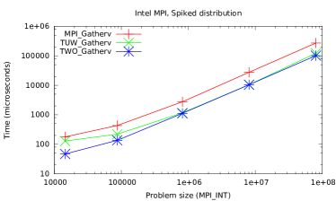
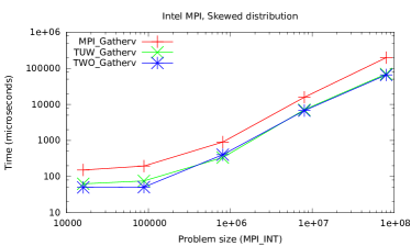
Figure 10: Running times of three different irregular gather implementations MPI_Gatherv, TUW_Gatherv, and TWO_Gatherv with $p=500\times 16=8000$ processes on an Intel/InfiniBand cluster with the Intel MPI library. Minimum completion times over 75 repetitions are in microseconds ($\mu s$), problem sizes in number of MPI_INT elements, doubly logarithmic plot.

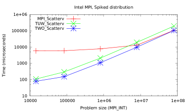
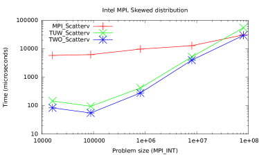
Figure 11: Running times of three different irregular scatter implementations MPI_Scatterv, TUW_Scatterv, and TWO_Scatterv with $p=500\times 16=8000$ processes on an Intel/InfiniBand cluster with the Intel MPI library. Minimum completion times over 75 repetitions are in microseconds ($\mu s$), problem sizes in number of MPI_INT elements, doubly logarithmic plot.

We finally investigate whether there are cases where non-binomial, optimal trees can do better than the adaptive binomial trees described and evaluated in [20] when implemented for a real system for and in MPI. We look at specific gather/scatter problems where it is obvious that the smallest completion time trees are not binomial. This is captured in Lemma 2.

Lemma 2

Let $x$ and $y$ be two distinct block sizes, $x<y$, for a gather or scatter problem with block sizes $m_{i},0\leq i<p$ with $m_{r}=y$ for exactly one $r$ and $m_{i}=x$ for all other $i\neq r$, such that the size of the problem is $m=(p-1)x+y$. Let $\alpha,\beta,\gamma$ be the communication parameters of a homogeneous system with $\gamma=\beta$. If $\lceil\log(p-1)\rceil\alpha+\beta(p-1)x\leq\beta y$, the cost of an optimal gather or scatter tree is $\alpha+\beta m$, and smaller than $\lceil\log p\rceil\alpha+\beta m$.

Proof: By Proposition 1, a tree of cost at most $\lceil\log(p-1)\rceil\alpha+\beta(p-1)x$ exists over the processors with $m_{i}=x$. Concurrently, the processor with $m_{r}=y$ can perform its local copy which takes $\beta y$, after which transmission between the roots of the two trees take place. Since there is only one communication latency to be accounted for in this tree, no better, lower latency tree can exist since also $p>1$. Any tree where the block $m_{r}$ is transmitted will have cost $\alpha+\beta m_{r}$ plus the cost of the other blocks, and thus larger. $\Box$

The argument assumes that processors can be freely ordered such that the $x$ and $y$ trees can be handled concurrently. If ordered gather or scatter trees are required, this is only possible if either $m_{0}=y$ or $m_{p-1}=y$, otherwise at least two communication operations will be required. This again shows that ordered trees can be slower than non-ordered trees. The dynamic programming algorithms would produce the best possible, ordered trees for such problem instances.

For problems with only two block sizes, optimal trees as outlined in Lemma 2 can readily be implemented by two concurrent gather or scatter operations on the domains of small and large blocks, respectively, and a single point-to-point communication. Since both gather/scatter operations are regular (small or large blocks), we can use the best implementations available for these problem, e.g., the library native MPI_Gather and MPI_Scatter operations. We use these implementations which we call TWO_Gatherv and TWO_Scatterv for the Spikes and Skewed distributions to compare against MPI library native MPI_Gatherv and MPI_Scatterv operations, and against implementations of the adaptive binomial tree algorithm called TUW_Gatherv and TUW_Scatterv [20]. We have done experiments on a medium-large Intel/InfiniBand cluster with 2000 Dual Intel Xeon E5-2650v2 8-core processors running at 2.6GHz, interconnected with an InfiniBand QDR-80 network. The MPI library is the native Intel MPI version 2018, and we choose the binomial tree algorithm for MPI_Gatherv and the linear algorithm for MPI_Scatterv which seemed to be the best performing available implementations in this library. We used $p=8000$ MPI processes on 500 nodes with 16 processes running on each.

Results for $b=1,10,100,1000,10000$ are plotted in Figure 10 and Figure 11, and show that optimal trees can perform better than binomial trees by a significant percentage, in the experiments with the Spikes scatter problems ranging from 25% to 50%. The poor performance of MPI_Scatterv on this system is due to a linear algorithm, which is clearly not the right choice for small(er), irregular scatter problems.

6 Concluding remarks

This paper investigated the irregular scatter and gather collective communication operations, both with respect to completion times for the operations, as well as with respect to the difficulty of finding communication trees leading to good completion times. The results under a synchronous, one-ported point-to-point communication model show that there is a difference in both respects between ordered and non-ordered communication trees as introduced here: Strongly ordered, minimal completion time trees can be computed in polynomial time, whereas constructing possibly better, non-ordered trees is NP-hard. We implemented dynamic programming algorithms for computing optimal ordered trees, and compared the quality (completion times) of the constructed trees for a set of different problem data block distributions. Based on these experiments, the problem-dependent, adaptive binomial tree construction which can compute trees fast in a distributed manner [20] can be seen to produce ordered trees that are very close to the optimal completion time trees and probably sufficient for all practical purposes. However, experiments with a real implementation for specially structured problems show that there are practical cases where optimal algorithms can do significantly better. This leaves room for devising practical algorithms that come still closer to the optimum solutions.

A number of interesting open problems has emerged that it would be worthwhile and fruitful to pursue further.

• Can the dynamic programming constructions be improved and extended? Monotonicity properties in the gather and scatter trees can possibly lower the complexity. Which alternative approaches can possibly lead to optimal or approximately optimal trees?

• What is the complexity of constructing weakly ordered communication trees, even in the one-ported model? Weakly ordered gather and scatter trees store consecutive segments of data blocks at all processors, but allow segments to be communicated in any order, not strictly in increasing rank order as required by the strictly ordered trees. Resolving this question could throw light on the problems in more asynchronous communication models.

• Under what conditions are trees not optimal communication structures for the gather and scatter problems? When might directed acyclic graphs (DAGs) perform better? How can such DAGs be constructed?

• How difficult are the problems with $k>1$ communication ports? How difficult are the problems under asynchronous communication models permitting overlap of communication operations?

Table 2: Gather tree completion times for ultra low latency network, $p=2000,b=1000,r=\lfloor p/2\rfloor,\rho=5,\alpha=1,\beta=1,\gamma=1,0$. For the different tree constructions, both the cases where the root $r$ is given externally (first row), and the case where a best root is chosen by the algorithm (second row) are shown. For the latter, the chosen root $(r)$ is given in brackets.

$\gamma=1$	$m$	Linear	($r$)	Binary	($r$)	Oblivious	($r$)	Adaptive	($r$)	Optimal	($r$)
Same	2000000	2001999		3610016		2000011		2000011		2000011
	2000000	2001999	(0)	3226015	(0)	2000011	(0)	2000011	(1023)	2000011	(1998)
Random	1983668	1985667		3586046		2030136		1993762		1983680
	1983668	1985667	(0)	3196585	(753)	2020053	(511)	1983679	(331)	1983679	(1171)
Random	1983668	1985667		4374656		2338418		2248476		1983680
decreasing	1983668	1985667	(0)	3192367	(0)	1983679	(0)	1983679	(1)	1983678	(0)
Random	1983668	1985667		3881291		3022129		2929259		1983680
increasing	1983668	1985667	(0)	3199725	(1236)	2076549	(1999)	1983679	(1791)	1983678	(1998)
Bucket	2005668	2007667		3612247		2032024		2012762		2005680
	2005668	2007667	(0)	3233050	(0)	2032024	(0)	2005679	(215)	2005679	(682)
Spikes	2001600	2003599		3567899		2141583		2036604		2001613
	2001600	2003599	(0)	3217645	(775)	2131633	(1999)	2001611	(1549)	2001610	(1198)
Decreasing	2003000	2004999		4415103		2352535		2265155		2003012
	2003000	2004999	(0)	3223175	(0)	2003011	(0)	2003011	(1)	2003010	(0)
Increasing	2003000	2004999		3915600		3047491		2954363		2003012
	2003000	2004999	(0)	3232091	(1999)	2096139	(1999)	2003011	(1791)	2003010	(1998)
Alternating	2000000	2001999		3609016		2000011		2000011		2000011
	2000000	2001999	(0)	3226015	(0)	2000011	(0)	2000011	(1023)	2000011	(1998)
Skewed	2001995	2003994		4402995		17201968		4002001		2002010
	2001995	2003994	(0)	2401998	(0)	2002006	(0)	2002006	(3)	2001998	(2)
Two blocks	2000000	2000002		3000002		11000011		3000002		2000002
	2000000	2000001	(0)	2000001	(0)	2000001	(0)	2000001	(1999)	2000001	(0)
$\gamma=0$	$m$	Linear	($r$)	Binary	($r$)	Oblivious	($r$)	Adaptive	($r$)	Optimal	($r$)
Same	2000000	2000999		3608016		1999011		1999011		1999011
	2000000	2000999	(0)	3225015	(0)	1999011	(0)	1999011	(1023)	1999011	(1998)
Random	1983668	1984973		3578075		2028324		1991822		1982985
	1983668	1983997	(1996)	3190317	(0)	2018241	(511)	1981739	(330)	1981679	(891)
Random	1983668	1984688		4371920		2336421		2246476		1982701
decreasing	1983668	1983667	(0)	3190627	(0)	1981679	(0)	1981679	(0)	1981678	(0)
Random	1983668	1984688		3876934		3020146		2927474		1982701
increasing	1983668	1983667	(1999)	3194265	(1999)	2074566	(1999)	1981894	(1791)	1981681	(1998)
Bucket	2005668	2006474		3607205		2030782		2011266		2004487
	2005668	2006334	(1999)	3229693	(1999)	2030782	(0)	2004183	(215)	2004180	(891)
Spikes	2001600	2003598		3542954		2136583		2031604		2001610
	2001600	1998599	(1992)	3192623	(775)	2126633	(1999)	1996611	(1549)	1996610	(1198)
Decreasing	2003000	2003998		4412223		2350535		2263154		2002011
	2003000	2002998	(0)	3221689	(0)	2001010	(0)	2001010	(0)	2001009	(0)
Increasing	2003000	2003997		3911230		3045506		2952570		2002010
	2003000	2002998	(1999)	3226539	(1999)	2094154	(1999)	2001218	(1791)	2001010	(1998)
Alternating	2000000	2000499		3603016		1999511		1998511		1998511
	2000000	2000499	(0)	3221515	(0)	1999511	(0)	1998511	(1022)	1998511	(1998)
Skewed	2001995	2003993		4002994		16801968		3602001		2002007
	2001995	1603994	(0)	2001998	(0)	1602006	(0)	1602006	(3)	1601998	(2)
Two blocks	2000000	2000002		2000002		11000011		2000002		2000002
	2000000	1000001	(0)	1000001	(0)	1000001	(0)	1000001	(1999)	1000001	(0)

Table 3: Gather tree completion times for high latency network, $p=2000,b=1000,r=\lfloor p/2\rfloor,\rho=5,\alpha=1000,\beta=1,\gamma=1,0$. For the different tree constructions, both the cases where the root $r$ is given externally (first row), and the case where a best root is chosen by the algorithm (second row) are shown. For the latter, the chosen root $(r)$ is given in brackets.

$\gamma=1$	$m$	Linear	($r$)	Binary	($r$)	Oblivious	($r$)	Adaptive	($r$)	Optimal	($r$)
Same	2000000	3999000		3626000		2011000		2011000		2011000
	2000000	3999000	(0)	3241000	(0)	2011000	(0)	2011000	(1023)	2011000	(1998)
Random	1983668	3982668		3601460		2041125		2004751		1995061
	1983668	3982668	(0)	3211992	(753)	2031042	(511)	1994668	(331)	1994668	(1014)
Random	1983668	3982668		4389641		2349407		2259465		1994878
decreasing	1983668	3982668	(0)	3206353	(0)	1994668	(0)	1994668	(1)	1993884	(0)
Random	1983668	3982668		3896276		3033118		2940248		1994878
increasing	1983668	3982668	(0)	3216898	(1236)	2087538	(1999)	1994668	(1791)	1993884	(1998)
Bucket	2005668	4004668		3627966		2043013		2023751		2017333
	2005668	4004668	(0)	3248035	(0)	2043013	(0)	2016668	(215)	2016668	(1006)
Spikes	2001600	4000600		3583827		2152572		2047593		2014600
	2001600	4000600	(0)	3232618	(775)	2142622	(1999)	2012600	(1549)	2011600	(1198)
Decreasing	2003000	4002000		4430088		2363524		2276144		2014256
	2003000	4002000	(0)	3237161	(0)	2014000	(0)	2014000	(1)	2013649	(0)
Increasing	2003000	4002000		3930239		3058480		2965352		2014256
	2003000	4002000	(0)	3247473	(1233)	2107128	(1999)	2014000	(1791)	2013649	(1998)
Alternating	2000000	3999000		3625000		2011000		2011000		2011000
	2000000	3999000	(0)	3241000	(0)	2011000	(0)	2011000	(1023)	2011000	(1998)
Skewed	2001995	4000995		4407990		17212957		4012990		2016995
	2001995	4000995	(0)	2404995	(0)	2012995	(0)	2012995	(3)	2004995	(2)
Two blocks	2000000	2002000		3002000		11011000		3002000		2002000
	2000000	2001000	(0)	2001000	(0)	2001000	(0)	2001000	(1999)	2001000	(0)
$\gamma=0$	$m$	Linear	($r$)	Binary	($r$)	Oblivious	($r$)	Adaptive	($r$)	Optimal	($r$)
Same	2000000	3998000		3624000		2010000		2010000		2010000
	2000000	3998000	(0)	3240000	(0)	2010000	(0)	2010000	(1023)	2010000	(1998)
Random	1983668	3981974		3594007		2039313		2002811		1994014
	1983668	3980998	(1996)	3205203	(0)	2029230	(511)	1992728	(330)	1992668	(891)
Random	1983668	3981689		4386905		2347410		2257465		1993877
decreasing	1983668	3980668	(0)	3204613	(0)	1992668	(0)	1992668	(0)	1992154	(0)
Random	1983668	3981689		3891919		3031135		2938463		1993877
increasing	1983668	3980668	(1999)	3211188	(1999)	2085555	(1999)	1992883	(1791)	1992157	(1998)
Bucket	2005668	4003475		3622985		2041771		2022255		2015857
	2005668	4003335	(1999)	3244678	(1999)	2041771	(0)	2015172	(215)	2015169	(891)
Spikes	2001600	4000599		3559937		2147572		2042593		2012599
	2001600	3995600	(1992)	3208607	(775)	2137622	(1999)	2007600	(1549)	2006600	(1198)
Decreasing	2003000	4000999		4427208		2361524		2274143		2013179
	2003000	3999999	(0)	3235675	(0)	2011999	(0)	2011999	(0)	2011712	(0)
Increasing	2003000	4000998		3925677		3056495		2963559		2013179
	2003000	3999999	(1999)	3241774	(1999)	2105143	(1999)	2012207	(1791)	2011713	(1998)
Alternating	2000000	3997500		3619000		2010500		2009500		2009500
	2000000	3997500	(0)	3236500	(0)	2010500	(0)	2009500	(1022)	2009500	(1998)
Skewed	2001995	4000994		4007989		16812957		3612990		2014994
	2001995	3600995	(0)	2004995	(0)	1612995	(0)	1612995	(3)	1604995	(2)
Two blocks	2000000	2002000		2002000		11011000		2002000		2002000
	2000000	1001000	(0)	1001000	(0)	1001000	(0)	1001000	(1999)	1001000	(0)

References

- [1] Albert Alexandrov, Mihai F. Ionescu, Klaus E. Schauser, and Chris J. Scheiman. LogGP: Incorporating long messages into the LogP model for parallel computation. Journal of Parallel and Distributed Computing, 44(1):71–79, 1997.
- [2] Sandeep N. Bhatt, Geppino Pucci, Abhiram Ranade, and Arnold L. Rosenberg. Scattering and gathering messages in networks of processors. IEEE Transactions on Computers, 42(8):938–949, 1993.
- [3] Jehoshua Bruck, Ching-Tien Ho, Schlomo Kipnis, Eli Upfal, and D. Weathersby. Efficient algorithms for all-to-all communications in multiport message-passing systems. IEEE Transactions on Parallel and Distributed Systems, 8(11):1143–1156, 1997.
- [4] Ernie Chan, Marcel Heimlich, Avi Purkayastha, and Robert A. van de Geijn. Collective communication: theory, practice, and experience. Concurrency and Computation: Practice and Experience, 19(13):1749–1783, 2007.
- [5] Ernie Chan, Robert A. van de Geijn, William Gropp, and Rajeev Thakur. Collective communication on architectures that support simultaneous communication over multiple links. In ACM SIGPLAN Symposium on Principles and Practice of Parallel Programming (PPoPP), pages 2–11, 2006.
- [6] Thomas H. Cormen, Charles E. Leiserson, Ronald L. Rivest, and Clifford Stein. Introduction to Algorithms. MIT Press, third edition, 2009.
- [7] Kiril Dichev, Vladimir Rychkov, and Alexey L. Lastovetsky. Two algorithms of irregular scatter/gather operations for heterogeneous platforms. In Recent Advances in the Message Passing Interface. 17th European MPI Users’ Group Meeting (EuroMPI), volume 6305 of Lecture Notes in Computer Science, pages 289–293. Springer, 2010.
- [8] Tarek El-Ghazawi, William Carlson, Thomas Sterling, and Katherine Yelick. UPC: Distributed Shared Memory Programming. John Wiley & Sons, 2005.
- [9] Pierre Fraigniaud and Emmanuel Lazard. Methods and problems of communication in usual networks. Discrete Applied Mathematics, 53(1–3):79–133, 1994.
- [10] M. R. Garey and D. S. Johnson. Computers and Intractability: A Guide to the Theory of NP-Completeness. Freeman, 1979. With an addendum, 1991.
- [11] S. Lennart Johnsson and Ching-Tien Ho. Optimum broadcasting and personalized communication in hypercubes. IEEE Transactions on Computers, 38(9):1249–1268, 1989.
- [12] Thilo Kielmann, Henri E. Bal, Sergei Gorlatch, Kees Verstoep, and Rutger F. H. Hofman. Network performance-aware collective communication for clustered wide-area systems. Parallel Computing, 27(11):1431–1456, 2001.
- [13] Damián A. Mallón, Guillermo L. Taboada, and Lars Koesterke. MPI and UPC broadcast, scatter and gather algorithms in Xeon Phi. Concurrency and Computation: Practice and Experience, 28(8):2322–2340, 2016.
- [14] MPI Forum. MPI: A Message-Passing Interface Standard. Version 3.1, June 4th 2015. www.mpi-forum.org.
- [15] Jarek Nieplocha, Bruce Palmer, Vinod Tipparaju, Manojkumar Krishnan, Harold Trease, and Edoardo Aprà. Advances, applications and performance of the global arrays shared memory programming toolkit. International Journal on High Performance Computing Applications, 20(2):203–231, 2006.
- [16] Paul Sack and William Gropp. Collective algorithms for multiported torus networks. ACM Transactions on Parallel Computing, 1(2):12:1–12:33, 2015.
- [17] Peter J. Slater, Ernest J. Cockayne, and Stephen T. Hedetniemi. Information dissemination in trees. SIAM Journal on Computing, 10(4):692–701, 1981.
- [18] Rajeev Thakur, William D. Gropp, and Rolf Rabenseifner. Improving the performance of collective operations in MPICH. International Journal on High Performance Computing Applications, 19:49–66, 2005.
- [19] Jesper Larsson Träff. Hierarchical gather/scatter algorithms with graceful degradation. In 18th International Parallel and Distributed Processing Symposium (IPDPS), page 80, 2004.
- [20] Jesper Larsson Träff. Practical, distributed, low overhead algorithms for irregular gather and scatter collectives. Parallel Computing, 75:100–117, 2018.
- [21] Yili Zheng, Amir Kamil, Michael B. Driscoll, Hongzhang Shan, and Katherine A. Yelick. UPC++: A PGAS extension for C++. In 28th IEEE International Parallel and Distributed Processing (IPDPS), pages 1105–1114, 2014.