Casimir Polder size consistency – a constraint violated by some dispersion theories

Abstract

A key goal in quantum chemistry methods, whether ab initio or otherwise, is to achieve size consistency. In this manuscript we formulate the related idea of “Casimir-Polder size consistency” that manifests in long-range dispersion energetics. We show that local approximations in time-dependent density functional theory dispersion energy calculations violate the consistency condition because of incorrect treatment of highly non-local “xc kernel” physics, by up to 10% in our tests on closed-shell atoms.

Quantum chemical approaches and electronic structure theories more generally aim to reproduce the key energetic physics of electrons with the goal of calculating energies for systems of interest. To a leading approximation two infinitely-separated quantum systems should have an energy that is given by the sum of the energies of the two components calculated separately – a feature known as size consistency. Thus, quantum chemistry methods are generally expected to reproduce this important property of quantum mechanics. Although its violation is sometimes tolerated (see e.g. Nooijen et al.¹) for greater accuracy or lower cost, it is nonetheless broadly accepted that size consistency is an important goal in method development as it captures a fundamental property of electronic systems.

The size consistency concept does not just apply at leading order, however. As two systems $A$ and $B$ approach each other, additional terms contribute to the energy, and these terms depend on properties of the isolated individual systems and the distance $D$ between them. As $D\to\infty$, the energy may thus be written as

$$E^{AB}(D)\sim E^{A}+E^{B}+U^{AB}(D).$$ (1)

where the potential energy

$$U^{AB}(D)\sim \sum_{p\geq 1}\frac{-C_{p}[\{\mathcal{L}^{A}\},\{\mathcal{L}^{B}\}]}{D^{p}}$$ (2)

depends in some factorizable way only on local properties $\mathcal{L}_{p}^{X}$ of the isolated systems $X=A,B$. Thus, e.g. for systems with net local charges $Q^{A}$ and $Q^{B}$, we have a leading term $U^{AB}(D)\to Q^{A}Q^{B}/D$ (i.e $C_{1}=-Q^{A}Q^{B}$).

Dipoles and higher multipoles yield similar expressions but with larger exponents $p>1$ and thus decay more rapidly. These static and multipolar contributions, including the static induction energy, are present at the electrostatic level and are properly included, via the Hartree energy, in all size consistent quantum chemical approximations the authors could think of. Note that induction is sometimes considered to be a correlation effect. Here we consider it to be an electostatic effect as it is present at the self-consistent Hartree level, unlike dispersion.

The leading beyond-electrostatic term is the attractive London dispersion (van der Waals) potential $U^{AB}_{\text{disp}}(D)=-C_{6}D^{-6}$, which is also the dominant asymptotic term for finite neutral systems without a permanent dipole or quadrupole. The coefficient,

$$C_{6,\text{CP}}= \int_{0}^{\infty}\frac{d\omega}{\pi}3\alpha^{A}(i\omega)\alpha^{B}(i\omega),$$ (3)

is obtained using an expression known as the Casimir-Polder formula² that is in the general form of (2). Eq. (3) can also be obtained by calculating $C_{6,\text{CP}}^{AB}=-\lim_{D\to\infty}D^{6}U^{AB}_{\text{CP}}(D)$ from

$$U^{AB}_{\text{CP}}= -\int_{0}^{\infty}\frac{d\omega}{2\pi}\text{Tr}\big{[}\hat{\chi}^{A}\hat{v}^{AB}\hat{\chi}^{B}\hat{v}^{BA}\big{]}\;,$$ (4)

sometimes called the generalized Casimir-Polder formula³ which applies to more general geometries. In this form it involves the anistropic density-density imaginary-frequency linear response functions $\hat{\chi}^{A/B}\equiv\hat{\chi}^{A/B}(i\omega)$ of the isolated systems, and the Coulomb potential $\hat{v}^{AB/BA}$ between them. Here and henceforth, products $\hat{G}\hat{H}=\int d\mathbf{r}G(\mathbf{r}_{1},\mathbf{r})H(\mathbf{r},\mathbf{r}_{2})$ indicate convolutions over space variables and the trace $\text{Tr}[\hat{G}]\equiv\int G(\mathbf{r},\mathbf{r})d\mathbf{r}$ is similarly defined.

Here the local variable $\mathcal{L}^{X}\equiv\alpha^{X}(i\omega)=-\frac{1}{3}\text{Tr}[(xx^{\prime}+yy^{\prime}+zz^{\prime})\hat{\chi}]$, from (2), is the spherically averaged imaginary-frequency dipole polarizability of the system $X$ and depends only on properties of $X$ calculated in isolation. Eq. (3) has proved to be exceedingly useful in practical calculations of dispersion forces^{4, 5, 6, 7, 8, 9, 10, 11, 12, 13, 14, 15}, which have been attracting much interest lately (see e.g. refs. [ 16, 17, 18, 19] and references therein) because of their increasingly recognised role in the behaviour of multiple chemical and material science processes.

Alternatively, we can adopt a direct route to calculating dispersion energies. We recognise that dispersion forces are a purely correlation effect – that is, they are absent in the Hartree and exchange energy terms which capture all electrostatic effects, at least for closed shell systems. Thus, $U^{AB}_{\text{disp}}(D)=E_{\text{c}}^{AB}(D)-E_{\text{c}}^{A}-E_{\text{c}}^{B}\to-C_{6}/D^{6}$, giving

$$C_{6,E_{\text{c}}}= -\lim_{D\to\infty}D^{6}\big{[}E_{\text{c}}^{AB}(D)-E_{\text{c}}^{A}-E_{\text{c}}^{B}\big{]}$$ (5)

where we calculate $E_{\text{c}}^{AB}$ for the combined system $AB$ separated at distance $D$. Thus, any method that can calculate correlation energies can be used to determine $C_{6}$ coefficients.

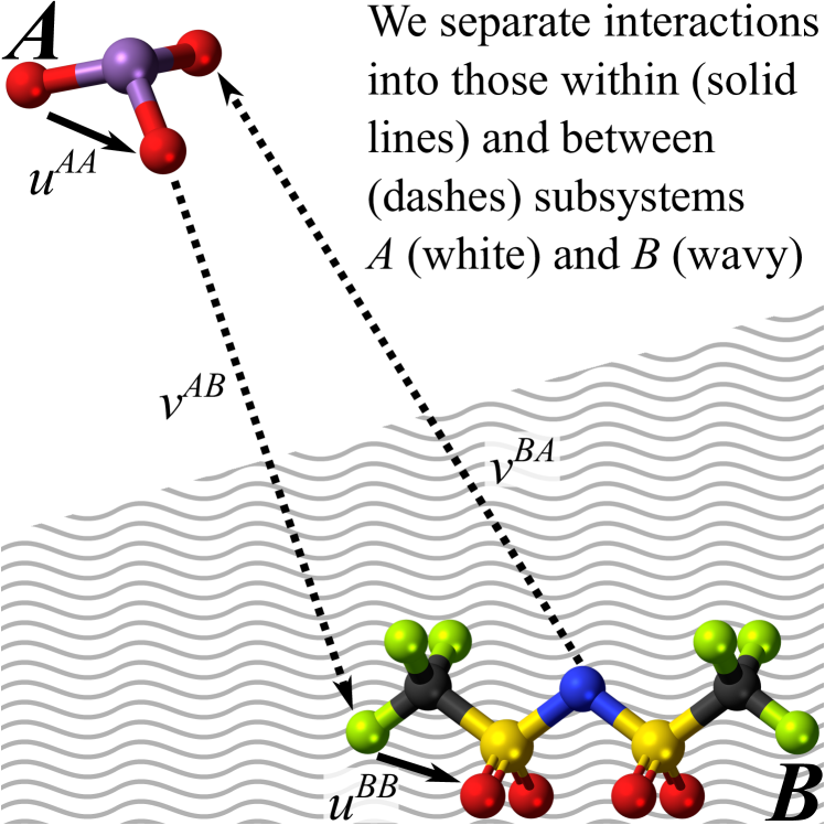
Figure 1: Interactions occur within ($u^{AA}$, $u^{BB}$) and between ($v^{AB}$, $v^{BA}$) systems $A$ and $B$. Switching off $v^{AB}/v^{BA}$ isolates the two systems.

This work now proceeds to formulate the idea of size consistency of dispersion forces, called “Casimir-Polder size consistency”²⁰. Then, it will show how time-dependent density functional theory²¹ approximations can violate Casimir-Polder size consistency. Next, it will give some examples illustrating the magnitude of the effect. Finally, some conclusions will be drawn and impact discussed.

Let us first define Casimir-Polder size consistency. Equations (3) and (5) are obtainable from first principles and thus should give the same result, i.e. coefficients obtained from the Casimir-Polder formula should be the same as those obtained from direct energy calculations. Thus any theory for which (3) equals (5) is Casimir-Polder size consistent. Any approximation where they are different is not Casimir-Polder size consistent and violates a fundamental property of well-separated systems.

We shall now proceed to show that, in time-dependent density functional theory (TDDFT) calculations of dispersion energies with a local exchange kernel, the two approaches give different results, and thus such theories are not Casimir-Polder size consistent. Furthermore, other high-level quantum chemical approaches based on screened response formalisms are also unlikely to be Casimir-Polder size consistent. Such approaches are attracting interest^{22, 23, 24, 25, 26, 27, 28, 29} because of their seamless inclusion of correlation physics, ability to deal with metals and gapped systems, and moderate cost. Any inconsistencies highlight a formal weakness of such approaches.

TDDFT offers two routes to dispersion energies. Firstly, it can be used to calculate dipole polarizabilities for use in the Casimir-Polder formula [Eq. (3)], or the density-density linear response functions for (4). Secondly, it can be used to obtain correlation energies by using the adiabatic connection formula³⁰ and fluctuation dissipation theorem (ACFD). Energies thus obtained include dispersion forces seamlessly^{31, 32, 18} [through Eq. (5)], making ACFD very useful for systems where dispersion competes with other effects, in stark contrast to semi-local theories which do not include any long-range dispersion.

It thus serves as a go-to approach for attacking dispersion calculations when beyond-empirical accuracy is required, but when more advanced quantum mechanical methods are infeasible. For example, TDDFT has been used to calculate $C_{6}$ coefficients of open shell atoms and ions, giving good agreement with experiment and more advanced methods^{33, 14}. A growing number of researchers are using TDDFT and ACFD for increasingly complex calculations^{18, 34, 35, 25, 26, 27, 28, 29} that are not yet feasible in wavefunction methods.

Table 1: $C_{6}$ coefficients calculated using ALDAx in Eqs. (3) and (5). $\Delta C_{6}$ quantifies the Casimir-Polder size consistency violation.

	He	Be	Ne	Mg	Ar	Ca	Zn	Kr
Eq. (3)	1.39	260	5.62	695	63.7	2420	349	132
Eq. (5)	1.37	235	5.59	635	63.0	2170	332	130
$\Delta C_{6}$	1.0%	9.5%	0.5%	8.6%	1.1%	10.5%	4.9%	1.3%

The ACFD correlation energy,

$$E_{\text{c}}^{\text{ACFD}}= -\int_{0}^{1}d\lambda\int_{0}^{\infty}\frac{d\omega}{2\pi}\text{Tr}\big{[}(\hat{\chi}_{\lambda}-\hat{\chi}_{0})\hat{v}\big{]}$$ (6)

of an electronic system is given in terms of $\hat{\chi}_{0}$, the linear response of its density to changes in the effective potential $\hat{v}_{s}$; and $\hat{\chi}_{\lambda}$, the equivalent linear response to an external potential at variable electron-electron interaction strength $\lambda$. Notably, $\hat{\chi}_{1}$ is the response of the real system to the external potential, and is the density-density linear response used in (4).

The relationship between these response functions is $\hat{\chi}_{\lambda}=\hat{\chi}_{0}+\hat{\chi}_{0}[\lambda(\hat{v}+\hat{f}_{\text{x}})+\hat{f}_{\text{c},\lambda}]\hat{\chi}_{\lambda}$, where all terms depend a priori on $\mathbf{r}$, $\mathbf{r}^{\prime}$ and $i\omega$, except for the Coulomb potential $\hat{v}=1/|\mathbf{r}-\mathbf{r}^{\prime}|$ which does not depend on $i\omega$. $\hat{f}_{\text{x}}$ is the exchange kernel,^{36, 37, 38, 39, 40, 41, 24} which is usually approximated. Finally, the correlation kernel $\hat{f}_{\text{c},\lambda}$²¹ is defined similarly to $\hat{f}_{\text{x}}$, but shall be assumed to be zero throughout this manuscript.

We have so far kept the ACFD general. Let us now consider specifically the $AB$ system, and introduce the “locality” assumption that occurs in most TDDFT approximations, i.e. that the exchange kernel is short-ranged in $|\mathbf{r}-\mathbf{r}^{\prime}|$ and depends only on the properties of the local system. We first partition space, as illustrated in Figure 1, between systems $A$ and $B$ to define $\hat{u}=\sum_{X=A,B}(\hat{v}^{XX}+\hat{f}_{\text{x}}^{XX})\equiv\hat{u}^{AA}+\hat{u}^{BB}$, $\hat{u}_{\text{H}}=\sum_{X=A,B}\hat{v}^{XX}$ and $\hat{w}=\hat{v}^{AB}+\hat{v}^{BA}$. Here $\hat{u}$ captures all intra-system interactions from both the Coulomb $\hat{v}^{XX}$ (corresponding to $\hat{u}_{\text{H}}$) and exchange kernel $\hat{f}_{\text{x}}^{XX}$ terms, where $\hat{f}_{\text{x}}^{XX}$ depends on properties of system $X$ only. $\hat{w}$ includes just the long-ranged inter-system Coulomb interactions $\hat{v}^{AB}/\hat{v}^{BA}$ and thus contains all dependencies on $D$. Then, we write the bare response $\hat{\chi}_{0}=\hat{\chi}_{0}^{A}+\hat{\chi}_{0}^{B}$ as a sum of subsystem responses $\hat{\chi}_{0}^{X}$ calculated in isolation.

Note that for our present purposes we can now see that TDDFT offers a conceptual advantage over wavefunction methods: both the Casimir-Polder formula and the ACFD expression are well-defined for any given kernel. Thus we can unequivocally talk about a subsystem calculation of the polarizability, and a correlation energy calcuation of the supersystem, at the same level of theory i.e. for a given kernel approximation.

Now that the details of the different response functions and interactions have been established, we shall next proceed to show that coefficients calculated using Eq. (3) [via (4)] are inconsistent with coefficients obtained from (5) [via (6)] in a common class of approximations, which thus lack Casimir-Polder size consistency.

With the assumptions described above, the TDDFT equation for the response $\hat{\chi}_{\lambda\gamma}$ of the combined system, with intra-system interaction strength $\lambda$ and inter-system interaction strength $\gamma$, is

$$\hat{\chi}_{\lambda\gamma}= \hat{\chi}_{00}+\hat{\chi}_{00}(\lambda\hat{u}+\gamma\hat{w})\hat{\chi}_{\lambda\gamma}\;,$$ (7)

where the bare response is $\hat{\chi}_{00}\equiv\hat{\chi}_{0}=\hat{\chi}_{0}^{A}+\hat{\chi}_{0}^{B}$. Let us start with $\lambda=\gamma=0$ and first switch on the intra-system interaction $\lambda$ while keeping $\gamma=0$ (equivalent to $D\to\infty$), to obtain the isolated system response $\hat{\chi}_{\lambda 0}=\hat{\chi}_{\lambda 0}^{A}+\hat{\chi}_{\lambda 0}^{B}=\sum_{X}[1-\lambda\hat{\chi}_{00}^{X}\hat{u}^{X}]^{-1}\hat{\chi}_{00}^{X}$ from

$$\hat{\chi}_{\lambda 0}= \hat{\chi}_{00}+\lambda\hat{\chi}_{00}\hat{u}\hat{\chi}_{\lambda 0}\;.$$ (8)

Then we switch on the inter-system interaction $\gamma$ to obtain

$$\hat{\chi}_{\lambda\gamma}= \hat{\chi}_{\lambda 0}+\gamma\hat{\chi}_{\lambda 0}\hat{w}\hat{\chi}_{\lambda\gamma}\;.$$ (9)

It is readily verified that (7) is reproduced by substituting the solution of (8) into (9).

Next we use (6) to write

$$U^{AB}= E_{\text{c}}^{AB}-E_{\text{c}}^{A}-E_{\text{c}}^{B}=-\int_{0}^{\infty}\frac{d\omega}{2\pi}\int_{0}^{1}d\lambda\Theta_{\lambda}\;,$$

where the equivalence between $\gamma=0$ and $D\to\infty$ gives $\Theta_{\lambda}=\text{Tr}[\hat{\chi}_{\lambda\gamma}(\hat{u}_{\text{H}}+\hat{w})-\hat{\chi}_{\lambda 0}\hat{u}_{\text{H}}]_{\gamma=\lambda}$. Iteration of (9) to second order in $\gamma$ (since inter-system interactions $\hat{w}$ are small) then gives $\hat{\chi}_{\lambda\gamma}\approx\hat{\chi}_{\lambda 0}+\gamma\hat{\chi}_{\lambda 0}\hat{w}\hat{\chi}_{\lambda 0}+\gamma^{2}\hat{\chi}_{\lambda 0}\hat{w}\hat{\chi}_{\lambda 0}\hat{w}\hat{\chi}_{\lambda 0}$, and

$$\Theta_{\lambda}= \text{Tr}\big{[}\lambda\hat{\chi}_{\lambda 0}\hat{w}\hat{\chi}_{\lambda 0}\hat{w}+\lambda^{2}\hat{\chi}_{\lambda 0}\hat{w}\hat{\chi}_{\lambda 0}\hat{w}\hat{\chi}_{\lambda 0}\hat{u}_{\text{H}}\big{]}$$ (10)

to leading order. Here we dropped terms involving odd powers of $\hat{w}$ as these are exactly zero in the trace.

Let us now digress from the general formula to consider the direct random-phase approximation (dRPA) which is the most popular, albeit flawed, approach to the seamless calculation of molecular and material properties using ACFD^{42, 43, 44, 45, 46, 18, 35, 47}. The dRPA consists of totally neglecting the exchange-correlation kernel ($f_{\text{xc}}=0$), giving $\hat{u}=\hat{v}^{AA}+\hat{v}^{BB}\equiv\hat{u}_{\text{H}}$. Taking the total derivative of (8) gives $\partial_{\lambda}\hat{\chi}_{\lambda 0}=\hat{\chi}_{\lambda 0}\hat{u}_{\text{H}}\hat{\chi}_{\lambda 0}$ so that (10) becomes $\Theta_{\lambda}^{\text{dRPA}}=\frac{1}{2}\partial_{\lambda}\text{Tr}\big{[}\lambda^{2}\hat{\chi}_{\lambda 0}\hat{w}\hat{\chi}_{\lambda 0}\hat{w}\big{]}=\partial_{\lambda}(\lambda^{2}\text{Tr}[\hat{\chi}_{\lambda 0}^{A}\hat{w}^{AB}\hat{\chi}_{\lambda 0}^{B}\hat{w}^{BA}])$, since $\hat{w}$ cannot couple points in the same subsystem. The occurrence of a perfect $\lambda$ derivative can be derived as follows: i) recognise that the explicit $O(\lambda)$ term can be expanded as $\lambda\text{Tr}[\hat{\chi}_{\lambda 0}^{A}\hat{w}^{AB}\hat{\chi}_{\lambda 0}^{B}\hat{w}^{BA}+\text{$B\Leftrightarrow A$}]=2\lambda\text{Tr}[\hat{\chi}_{\lambda 0}^{A}\hat{w}^{AB}\hat{\chi}_{\lambda 0}^{B}\hat{w}^{BA}]$; ii) then use $\partial_{\lambda}\hat{\chi}_{\lambda 0}^{X}=\hat{\chi}_{\lambda 0}^{X}\hat{v}^{XX}\hat{\chi}_{\lambda 0}^{X}$ in the explicit $O(\lambda^{2})$ term to get $\lambda^{2}\text{Tr}[\hat{\chi}_{\lambda 0}^{A}\hat{w}^{AB}\hat{\chi}_{\lambda 0}^{B}\hat{v}^{BB}\hat{\chi}_{\lambda 0}^{B}\hat{w}^{BA}+\text{$B\Leftrightarrow A$}]=\lambda^{2}\text{Tr}[\hat{\chi}_{\lambda 0}^{A}\hat{w}^{AB}[\partial_{\lambda}\hat{\chi}_{\lambda 0}^{B}]\hat{w}^{BA}+\text{$B\Leftrightarrow A$}]$, which can be written using the cyclic properties of the trace as $\lambda^{2}\partial_{\lambda}\text{Tr}[\hat{\chi}_{\lambda 0}^{A}\hat{w}^{AB}\hat{\chi}_{\lambda 0}^{B}\hat{w}^{BA}]$; iii) add the two terms to get $\Theta_{\lambda}^{\text{dRPA}}=\partial_{\lambda}(\lambda^{2}\text{Tr}[\hat{\chi}_{\lambda 0}^{A}\hat{w}^{AB}\hat{\chi}_{\lambda 0}^{B}\hat{w}^{BA}])$, as desired.

Integrating over $\lambda$ then gives⁴⁸,

$$U^{AB}_{\text{dRPA}}= -\int_{0}^{\infty}\frac{d\omega}{2\pi}\text{Tr}\big{[}\hat{\chi}_{\text{dRPA}}^{A}\hat{v}^{AB}\hat{\chi}_{\text{dRPA}}^{B}\hat{v}^{BA}\big{]}\;,$$ (11)

to second order in $\hat{w}$, which is Eq. (4) calculated using $\hat{\chi}_{\text{dRPA}}^{X}\equiv[1-\hat{\chi}_{00}^{X}\hat{v}^{XX}]^{-1}\hat{\chi}_{00}^{X}$, the dRPA response of the isolated system with full-strength ($\lambda=1$) internal Coulomb interaction $\hat{v}^{XX}$. Thus the energy calculated using the dRPA on the total system [Eq. (5)] is the same as that calculated using the Casimir-Polder formula [Eq. (11) or (3)] with the dRPA response functions. The dRPA is Casimir-Polder size consistent²⁰.

However, the dRPA is crude and relies on a cancellation of short-range errors³² for its successes. Thus, work is ongoing to improve on the dRPA by modelling the kernel^{22, 23, 24, 25, 26, 27, 28, 29}. Let us now consider an exchange term $f_{\text{x}}$ in our intra-system interactions to get $\hat{u}=\hat{u}_{\text{H}}+\hat{f}_{\text{x}}$. Now, $\partial_{\lambda}\hat{\chi}_{\lambda 0}=\hat{\chi}_{\lambda 0}(\hat{u}_{\text{H}}+\hat{f}_{\text{x}})\hat{\chi}_{\lambda 0}$ and we get $\Theta_{\lambda}^{\text{x}}=\frac{1}{2}\partial_{\lambda}\text{Tr}\big{[}\lambda^{2}\hat{\chi}_{\lambda 0}\hat{w}\hat{\chi}_{\lambda 0}w\big{]}-\lambda^{2}\text{Tr}\big{[}\hat{\chi}_{\lambda 0}\hat{w}\hat{\chi}_{\lambda 0}w\hat{\chi}_{\lambda 0}\hat{f}_{\text{x}}\big{]}$ via a similar set of steps exhibited above for the dRPA.

Thus, in contrast to the dRPA, local TDDFT theories have an additional term $\Theta_{\lambda}$ that cannot be written as a derivative. After integration, the derivative term gives the expected Casimir-Polder formula of Eq. (3) calculated with the appropriate response $\hat{\chi}_{10}^{\text{x}}=[1-\hat{\chi}_{00}(\hat{u}_{\text{H}}+\hat{f}_{\text{x}})]^{-1}\hat{\chi}_{00}$ including the exchange kernel. The other term thus quantifies the violation of Casimir-Polder size consistency by the approximation, which we can express as

$$\Delta U^{AB}_{\text{x}} =\int_{0}^{\infty}\frac{d\omega}{2\pi}\int_{0}^{1}d\lambda\lambda^{2}\sum_{X=A,B}$$

$$\times\text{Tr}\big{[}\hat{\chi}_{\lambda 0}^{X}\hat{v}^{XY}\hat{\chi}^{Y}_{\lambda 0}\hat{f}^{YY}_{\text{x}}\hat{\chi}^{Y}_{\lambda 0}\hat{v}^{YX}\big{]}\;,$$ (12)

where $Y\neq X$ indicates the other system.

Eq. (12) represents the key theoretical result of this work, either directly or via its contribution $\Delta C_{6}^{\text{x}}=-\lim_{D\to\infty}D^{6}\Delta U_{\text{x}}^{AB}(D)$ to the $C_{6}$ coefficient. It illustrates that ACFD methods with beyond-Coulomb kernels acting within systems $A$ or $B$, but only Coulomb interactions acting between systems $A$ and $B$ can give rise to a difference in energies calculated using the Casimir-Polder formula versus a full correlation energy calculation of the $AB$ system. Such approaches are not Casimir-Polder size consistent and thus violate a fundamental quantum mechanical constraint.

We now investigate the magnitude of Eq. (12) on a selection of atomic systems using an adiabatic local density approximation⁴⁹ for the exchange kernel only (ALDAx). Thus, $f_{\text{x}}(\mathbf{r},\mathbf{r}^{\prime})\equiv\delta(\mathbf{r}-\mathbf{r}^{\prime})f_{\text{x}}^{\text{ALDA}}(n(\mathbf{r}))$ where $f_{\text{x}}^{\text{ALDA}}(n)$ is the second-order derivative of the exchange energy density of the homogeneous electron gas with respect to the density $n$. This kernel is chosen not for its accuracy, but because it, like all semi-local kernels, is obviously consistent with the assumptions we made about $\hat{u}^{XX}$ depending only on properties of system $X$, and $\hat{w}$ neglecting kernel terms entirely.

It is worth noting that the local kernel used here produces a divergent on-top correlation hole but a finite correlation energy. Our general form (12) is not restricted to such local kernels and can accommodate more accurate short-range physics. The size-consistency issue is related to the long-range physics, however, and is unlikely to be systematically improved through better short-range physics.

Table 1 reports $C_{6}$ values calculated (see Gould and Bučko¹⁴ for numerical details) using Eqs. (3) and (5) within ALDAx, and shows the difference as a percent. In some cases the difference between the $C_{6}$ coefficients derived from the Casimir-Polder formula and the energy of the system as a whole is substantial. For the highly polarizable alkaline earth metals it can be as much as 10% of the total coefficient, a difference similar to the predicted accuracy of TDDFT-derived coefficients¹⁴. By contrast, for noble gases the difference is $\sim\!\!1\%$, similar to numerical errors.

In conclusion, we have shown that local approximations to TDDFT kernels violate a constraint we call “Casimir-Polder size consistency”, because the dispersion $C_{6}$ coefficient calculated from properties of the two systems $A$ and $B$ [Eq. (3)] differs from that calculated, within the same approximations, from the two systems studied together [Eq. (5)]. This result is inconsistent with ideas of separability as manifested in Eqs. (1) and (2). In the worst cases tested here, alkaline earth atoms, we find significant deviations of $\sim\!\!10\%$ using an exchange-only adiabatic local density approximation. Worryingly, the deviation seems to affect the most polarizable atoms the most, suggesting its importance is amplified in the very systems where dispersion contributes most greatly to energetics.

Generalization of our results suggests that even sophisticated “local” correlation kernels (e.g. rALDA²⁵) cannot resolve the issue. We believe that similar problems will manifest in some time-dependent generalized Kohn-Sham schemes involving four-point kernels, although notably it was observed by Szabo and Ostlund⁵⁰ that a variant of RPA with a nonlocal Hartree-Fock exchange kernel is Casimir-Polder size consistent (see also the discussion in Ref.  51). Work is ongoing to elucidate more general cases, including important wavefunction methods.

Caution is thus advised when comparing long-range forces calculated using polarizabilities, or via systems as a whole. Such approaches include range-separated approaches.^{52, 53, 54, 51, 55} Guaranteeing Casimir-Polder size consistency should be a goal for new kernel approximations³. Similarly, one might look for response models that can reproduce by construction quantum chemical theories of supersystems and thus automatically avoid Casimir-Polder size consistency issues.

The authors wish to acknowledge the important contribution of our good friend and colleague, the late Prof. János Ángyán. This work would not exist without his efforts, and we are saddened he could not see it completed. T.G. received funding from a Griffith University International Travel Fellowship.

References

- Nooijen et al. 2005 Nooijen, M.; Shamasundar, K. R.; Mukherjee, D. Reflections on size-extensivity, size-consistency and generalized extensivity in many-body theory. Molecular Physics 2005, 103, 2277–2298
- Casimir and Polder 1948 Casimir, H. B. G.; Polder, D. The Influence of Retardation on the London-van der Waals Forces. Phys. Rev. 1948, 73, 360–372
- Kevorkyants et al. 2014 Kevorkyants, R.; Eshuis, H.; Pavanello, M. FDE-vdW: A van der Waals inclusive subsystem density-functional theory. J. Chem. Phys. 2014, 141, 044127
- Dobson et al. 2000 Dobson, J. F.; Dinte, B. P.; Wang, J.; Gould, T. A Novel Constraint for the Simplified Description of Dispersion Forces. Aus. J. Phys. 2000, 53, 575–596
- Dobson et al. 2001 Dobson, J. F.; McLennan, K.; Rubio, A.; Wang, J.; Gould, T.; Le, H. M.; Dinte, B. P. Prediction of Dispersion Forces: Is There a Problem? Aust. J. Chem. 2001, 54, 513–527
- Grimme 2004 Grimme, S. Accurate description of van der Waals complexes by density functional theory including empirical corrections. J. Comput. Chem. 2004, 25, 1463–1473
- Becke and Johnson 2005 Becke, A. D.; Johnson, E. R. Exchange-hole dipole moment and the dispersion interaction. J. Chem. Phys. 2005, 122, 154104
- Grimme 2006 Grimme, S. Semiempirical GGA-type density functional constructed with a long-range dispersion correction. J. Comp. Chem. 2006, 27, 1787–1799
- Tkatchenko and Scheffler 2009 Tkatchenko, A.; Scheffler, M. Accurate Molecular Van Der Waals Interactions from Ground-State Electron Density and Free-Atom Reference Data. Phys. Rev. Lett. 2009, 102, 073005
- Grimme et al. 2010 Grimme, S.; Antony, J.; Ehrlich, S.; Krieg, H. A consistent and accurate ab initio parametrization of density functional dispersion correction (DFT-D) for the 94 elements H-Pu. J. Chem. Phys. 2010, 132, 154104
- Tkatchenko et al. 2012 Tkatchenko, A.; DiStasio, R. A.; Car, R.; Scheffler, M. Accurate and Efficient Method for Many-Body van der Waals Interactions. Phys. Rev. Lett. 2012, 108, 236402
- Toulouse et al. 2013 Toulouse, J.; Rebolini, E.; Gould, T.; Dobson, J. F.; Seal, P.; Ángyán, J. G. Assessment of range-separated time-dependent density-functional theory for calculating dispersion coefficients. J. Chem. Phys. 2013, 138, 194106
- Gould 2016 Gould, T. How polarizabilities and coefficients actually vary with atomic volume. J. Chem. Phys. 2016, 145
- Gould and Bučko 2016 Gould, T.; Bučko, T. C6 Coefficients and Dipole Polarizabilities for All Atoms and Many Ions in Rows 1–6 of the Periodic Table. J. Chem. Theory Comput. 2016, 12, 3603–3613
- Gould et al. 2016 Gould, T.; Lebègue, S.; Ángyán, J. G.; Bučko, T. Many-body dispersion corrections for periodic systems: an efficient reciprocal space implementation. J. Chem. Theor. Comput. 2016, 12, 5920–5930
- Grimme 2011 Grimme, S. Density functional theory with London dispersion corrections. Wiley Interdisciplinary Reviews: Computational Molecular Science 2011, 1, 211–228
- Dobson and Gould 2012 Dobson, J. F.; Gould, T. Calculation of dispersion energies. J. Phys.: Condens. Matter 2012, 24, 073201
- Eshuis et al. 2012 Eshuis, H.; Bates, J. E.; Furche, F. Electron correlation methods based on the random phase approximation. Theor. Chem. Acc. 2012, 131, 1–18
- Woods et al. 2016 Woods, L.; Dalvit, D.; Tkatchenko, A.; Rodriguez-Lopez, P.; Rodriguez, A.; Podgornik, R. Materials perspective on Casimir and van der Waals interactions. Rev. Mod. Phys. 2016, 88, 045003
- Dobson 2012 Dobson, J. F. In Fundamentals of Time Dependent Density Functional Theory; Marques, M. A., Maitra, N. T., Nogueira, F. M., Gross, E. K., Rubio, A., Eds.; Springer Science & Business Media, 2012; Vol. 837
- Runge and Gross 1984 Runge, E.; Gross, E. K. U. Density-Functional Theory for Time-Dependent Systems. Phys. Rev. Lett. 1984, 52, 997–1000
- Petersilka et al. 1996 Petersilka, M.; Gossmann, U. J.; Gross, E. K. U. Excitation Energies from Time-Dependent Density-Functional Theory. Phys. Rev. Lett. 1996, 76, 1212–1215
- Gould 2012 Gould, T. Communication: Beyond the random phase approximation on the cheap: Improved correlation energies with the efficient “radial exchange hole” kernel. J. Chem. Phys. 2012, 137, 111101
- Hellgren and Gross 2013 Hellgren, M.; Gross, E. K. U. Discontinuous functional for linear-response time-dependent density-functional theory: The exact-exchange kernel and approximate forms. Phys. Rev. A 2013, 88, 052507
- Olsen and Thygesen 2013 Olsen, T.; Thygesen, K. S. Beyond the random phase approximation: Improved description of short-range correlation by a renormalized adiabatic local density approximation. Phys. Rev. B 2013, 88, 115131
- Heßelmann and Görling 2013 Heßelmann, A.; Görling, A. On the Short-Range Behavior of Correlated Pair Functions from the Adiabatic-Connection Fluctuation-Dissipation Theorem of Density-Functional Theory. J. Chem. Theory Comput. 2013, 9, 4382–4395, PMID: 26589155
- Jauho et al. 2015 Jauho, T. S.; Olsen, T.; Bligaard, T.; Thygesen, K. S. Improved description of metal oxide stability: Beyond the random phase approximation with renormalized kernels. Phys. Rev. B 2015, 92, 115140
- Dixit et al. 2016 Dixit, A.; Ángyán, J. G.; Rocca, D. Improving the accuracy of ground-state correlation energies within a plane-wave basis set: The electron-hole exchange kernel. J. Chem. Phys. 2016, 145, 104105
- Mussard et al. 2016 Mussard, B.; Rocca, D.; Jansen, G.; Ángyán, J. G. Dielectric Matrix Formulation of Correlation Energies in the Random Phase Approximation: Inclusion of Exchange Effects. J. Chem. Theory Comput. 2016, 12, 2191–2202
- Gunnarsson and Lundqvist 1976 Gunnarsson, O.; Lundqvist, B. I. Exchange and correlation in atoms, molecules, and solids by the spin-density-functional formalism. Phys. Rev. B 1976, 13, 4274–4298
- Dobson and Wang 1999 Dobson, J. F.; Wang, J. Successful Test of a Seamless van der Waals Density Functional. Phys. Rev. Lett. 1999, 82, 2123–2126
- Furche and Voorhis 2005 Furche, F.; Voorhis, T. V. Fluctuation-dissipation theorem density-functional theory. J. Chem. Phys. 2005, 122, 164106
- Chu and Dalgarno 2004 Chu, X.; Dalgarno, A. Linear response time-dependent density functional theory for van der Waals coefficients. J. Chem. Phys. 2004, 121, 4083–4088
- Ren et al. 2012 Ren, X.; Rinke, P.; Joas, C.; Scheffler, M. Random-phase approximation and its applications in computational chemistry and materials science. J. Mater. Sci. 2012, 47, 7447–7471
- Björkman et al. 2012 Björkman, T.; Gulans, A.; Krasheninnikov, A. V.; Nieminen, R. M. van der Waals Bonding in Layered Compounds from Advanced Density-Functional First-Principles Calculations. Phys. Rev. Lett. 2012, 108, 235502
- Görling 1998 Görling, A. Exact exchange kernel for time-dependent density-functional theory. Int. J. Quantum Chem. 1998, 69, 265–277
- Hellgren and von Barth 2008 Hellgren, M.; von Barth, U. Linear density response function within the time-dependent exact-exchange approximation. Phys. Rev. B 2008, 78, 115107
- Heßelmann and Görling 2010 Heßelmann, A.; Görling, A. Random phase approximation correlation energies with exact Kohn–Sham exchange. Mol. Phys. 2010, 108, 359–372
- Hellgren and von Barth 2010 Hellgren, M.; von Barth, U. Correlation energy functional and potential from time-dependent exact-exchange theory. J. Chem. Phys. 2010, 132, 044101
- Hellgren and Gross 2012 Hellgren, M.; Gross, E. K. U. Discontinuities of the exchange-correlation kernel and charge-transfer excitations in time-dependent density-functional theory. Phys. Rev. A 2012, 85, 022514
- Bleiziffer et al. 2012 Bleiziffer, P.; Heßelmann, A.; Görling, A. Resolution of identity approach for the Kohn-Sham correlation energy within the exact-exchange random-phase approximation. J. Chem. Phys. 2012, 136, 134102
- Dobson et al. 2006 Dobson, J. F.; White, A.; Rubio, A. Asymptotics of the dispersion interaction: analytic benchmarks for van der Waals energy functionals. Phys. Rev. Lett. 2006, 96, 073201
- Harl and Kresse 2008 Harl, J.; Kresse, G. Cohesive energy curves for noble gas solids calculated by adiabatic connection fluctuation-dissipation theory. Phys. Rev. B 2008, 77, 045136
- Grüneis et al. 2009 Grüneis, A.; Marsman, M.; Harl, J.; Schimka, L.; Kresse, G. Making the random phase approximation to electronic correlation accurate. J. Chem. Phys. 2009, 131, 154115
- Dobson et al. 2009 Dobson, J. F.; Gould, T.; Klich, I. Dispersion interaction between crossed conducting wires. Phys. Rev. A 2009, 80, 012506
- Lebègue et al. 2010 Lebègue, S.; Harl, J.; Gould, T.; Ángyán, J. G.; Kresse, G.; Dobson, J. F. Cohesive Properties and Asymptotics of the Dispersion Interaction in Graphite by the Random Phase Approximation. Phys. Rev. Lett. 2010, 105, 196401
- 47 Gould, T.; Lebègue, S.; Björkman, T.; Dobson, J. In 2D Materials; Francesca Iacopi, J. J. B., Jagadish, C., Eds.; Semiconductors and Semimetals; Elsevier, Vol. 95; pp 1–33
- Dobson 1994 Dobson, J. F. In Topics in Condensed Matter Physics; Das, M. P., Ed.; Nova Science Publisher, 1994; pp 121–142, Available as arXiv preprint cond-mat/0311371
- Zangwill and Soven 1980 Zangwill, A.; Soven, P. Resonant Photoemission in Barium and Cerium. Phys. Rev. Lett. 1980, 45, 204–207
- Szabo and Ostlund 1977 Szabo, A.; Ostlund, N. S. The correlation energy in the random phase approximation: Intermolecular forces between closed-shell systems. J. Chem. Phys. 1977, 67, 4351–4360
- Toulouse et al. 2011 Toulouse, J.; Zhu, W.; Savin, A.; Jansen, G.; Ángyán, J. G. Closed-shell ring coupled cluster doubles theory with range separation applied on weak intermolecular interactions. J. Chem. Phys. 2011, 135, 084119
- Toulouse et al. 2009 Toulouse, J.; Gerber, I. C.; Jansen, G.; Savin, A.; Ángyán, J. G. Adiabatic-connection fluctuation-dissipation density-functional theory based on range separation. Phys. Rev. Lett. 2009, 102, 096404
- Toulouse et al. 2010 Toulouse, J.; Zhu, W.; Ángyán, J. G.; Savin, A. Range-separated density-functional theory with the random-phase approximation: Detailed formalism and illustrative applications. Phys. Rev. A 2010, 82, 032502
- Zhu et al. 2010 Zhu, W.; Toulouse, J.; Savin, A.; Ángyán, J. G. Range-separated density-functional theory with random phase approximation applied to noncovalent intermolecular interactions. J. Chem. Phys. 2010, 132, 244108
- Ángyán et al. 2011 Ángyán, J. G.; Liu, R.-F.; Toulouse, J.; Jansen, G. Correlation Energy Expressions from the Adiabatic-Connection Fluctuation-Dissipation Theorem Approach. J. Chem. Theory Comput. 2011, 7, 3116