Landau levels in QCD in an external magnetic field

Abstract

We will discuss the issue of Landau levels of quarks in lattice QCD in an external magnetic field. We will show that in the two-dimensional case the lowest Landau level can be identified unambiguously even if the strong interactions are turned on. Starting from this observation, we will then show how one can define a "lowest Landau level" in the four-dimensional case, and discuss how much of the observed effects of a magnetic field can be explained in terms of it. Our results can be used to test the validity of low-energy models of QCD that make use of the lowest-Landau-level approximation.

1 Introduction

The effects of a background magnetic field on strongly interacting matter are relevant to a number of problems in particle physics, astrophysics and cosmology, see the recent reviews Kharzeev:2013jha ; Miransky:2015ava . In heavy ion collisions, the colliding ions generate strong magnetic fields that affect the quark-gluon plasma formed in the collision. Moreover, the equation of state of hadronic matter in an external magnetic field is needed in the study of magnetars (a type of neutron stars), and also in the study of the evolution of the early Universe. This provides enough motivation to study the phase diagram of QCD in an external, uniform magnetic field.

This task has been (partially) accomplished in recent years by means of numerical calculations from first principles on the lattice. Due to the yet unsolved sign problem at finite chemical potential, only the corner of the phase diagram at vanishing chemical potential can be reliably determined in this way. What is known in this case is that for temperatures well below and well above the QCD pseudocritical temperature $T_{c}$ at $B=0$, a constant magnetic field increases the quark condensate, a phenomenon dubbed magnetic catalysis (MC), while around $T_{c}$ it decreases the condensate, i.e., it gives inverse magnetic catalysis (IMC) Bali:2011qj . This results in $T_{c}$ decreasing with $B$. This behaviour was missed in early lattice studies DElia:2010abb , due to the fact that lattice artefacts can turn IMC into MC: fine lattices and physical quark masses are needed to observe IMC on the lattice.

An important question is how can these phenomena be understood in the framework of QCD. To this end, it is convenient to distinguish the two effects that an external magnetic field has on the formation of a quark condensate. The magnetic field appears in fact both in the operator being averaged (here the inverse of the Dirac operator) and in the fermionic determinant, i.e., in the functional integral measure. The presence of a magnetic field has been observed to increase the density of low modes of the Dirac operator in a typical gauge configuration: this effect, dubbed valence effect, tends to increase the condensate via the Banks-Casher relation, and therefore pushes in the direction of MC. On the other hand, configurations with a higher density of low modes are relatively suppressed because of the determinant: this tends to reduce the condensate and therefore goes in the direction of IMC. This is the so-called sea effect, which is typically weaker than the valence effect, so that in general one finds MC. Near $T_{c}$, though, where the Polyakov loop effective potential is flatter and so the sea effect is most effective, the latter ends up winning against the valence effect, therefore leading to IMC Bruckmann:2013oba .

IMC near $T_{c}$ was a quite unexpected result, given the pre-existing common lore based on analytic calculations in low-energy models for QCD, which predicted MC at all temperatures (see, e.g., the reviews Miransky:2015ava ; Shovkovy:2012zn ; Andersen:2014xxa ). The basis for this common lore is the expected behaviour of the lowest Landau level (LLL) of quarks in a constant magnetic field: as its degeneracy is proportional to the magnetic field, an increase in the density of low Dirac modes is expected. This would explain the valence effect, which is required for MC. In this framework, one expects that only the LLL is physically relevant for sufficiently large magnetic fields: this leads to the frequently used LLL approximation, where all higher Landau levels are neglected (see, e.g., Refs. Leung:2005xz ; Fayazbakhsh:2010gc ; Fukushima:2011nu ; Ferrer:2013noa ). However, in QCD quarks interact with the SU(3) gauge fields besides the external magnetic field, and therefore the very meaning of Landau levels is not obvious. In the rest of this proceeding we will discuss in detail how the LLL can be interpreted in this setup, how one can identify it on the lattice, and how much it actually contributes to the (change of the) chiral condensate in a magnetic field, so testing the validity of the LLL approximation. This work is based on the paper Bruckmann:2017pft .

2 Landau levels in the continuum

As is well known, Landau levels (LLs) are the energy levels of an otherwise free particle immersed in a uniform magnetic field $B$. For brevity, in the following we will refer to this simply as the “free case”. In the presence of interactions, one expects for weakly coupled particles that the LL structure gets only slightly perturbed. This has been verified on the lattice in the case of pions in the presence of both strong interactions and an external magnetic field Bali:2011qj . The LLs relevant to the problem of MC are however those of quarks with “Hamiltonian” given by the Dirac operator in the presence of non-Abelian gauge fields. Since quarks are strongly coupled to the non-Abelian gauge fields, the question of whether the LL structure survives the introduction of strong interactions is a rather nontrivial one.

We begin our discussion by reviewing the simplest possible case of spin-$\frac{1}{2}$ fermions of charge $q$ in the continuum, confined to live in a two-dimensional plane, and subject only to a uniform magnetic field orthogonal to that plane. In this case the eigenvalues $\lambda_{n}^{2}$ of $-{\not{D}}^{2}$ and their degeneracies $\nu_{n}$ read

$$\lambda^{2}_{n}=qBn\,,\qquad n=2k+1-2s_{z}\,,\qquad\nu_{n}=N_{b}(2-\delta_{0n})\,,$$ (1)

where $k=0,1,\ldots$, $s_{z}=\pm\frac{1}{2}$ is the spin of the particle along the direction of the magnetic field, and so $n=0,1,2,\ldots$, and where $N_{b}=\frac{L_{x}L_{y}qB}{2\pi}=\frac{\Phi_{B}}{2\pi}\in\mathbb{Z}$ due to the quantisation of the magnetic flux $\Phi_{B}$ in a finite volume. For quarks with $N_{c}$ colours one gets an extra factor $N_{c}$ in the degeneracies. The generalisation to quarks in four dimensions is easy. The eigenvalues get also contributions from the momenta in the $t$ and $z$ directions, while the degeneracies are doubled due to particle-antiparticle symmetry:

$$\lambda^{2}_{np_{z}p_{t}}=qBn+p_{z}^{2}+p_{t}^{2}\,,\qquad\nu_{n}=2N_{c}N_{b}(2-\delta_{0n})\,.$$ (2)

This result provides the basis for a simple argument for the valence effect and in favour of MC. If we believe that the LL structure is not affected very much by the strong interactions, then since the LLL is just at $\lambda=0$ one would expect an increase in the spectral density near the origin roughly proportional to $B$, and therefore an increase in the chiral condensate. Assuming that the LL structure is preserved is, however, quite a strong assumption that should be carefully tested on the lattice, especially in the light of the fact that quarks are strongly coupled.

3 Landau levels on the lattice: two-dimensional case

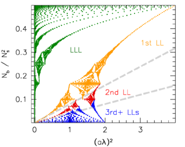
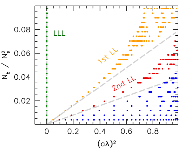
Figure 1: Classification of the lattice eigenvalues according to continuum Landau level degeneracies in the free case. Continuum Landau levels are shown as gray dashed lines. The right panel shows a zoom into the region around the origin, where the continuum Landau levels are approached.

Our next step is to study the two-dimensional case on the lattice, using the staggered Dirac operator $D_{\rm stag}$. This discretisation entails an exact twofold doubling of the squared eigenvalues, which in the continuum limit in the free case would lead to an extra factor of two in the degeneracy of the LLs. The results for the spectrum in the free case are well known (see Fig. 1): the eigenvalues spread around the continuum values due to lattice artefacts, and give rise to a fractal structure known in the condensed matter literature as Hofstadter’s butterfly Hofstadter:1976zz ; Endrodi:2014vza . The LL structure is spoiled by the lattice, but nevertheless a remnant of it still remains, as signalled by the presence of clear gaps between groups of eigenvalues that match in size the degeneracies of the continuum levels.

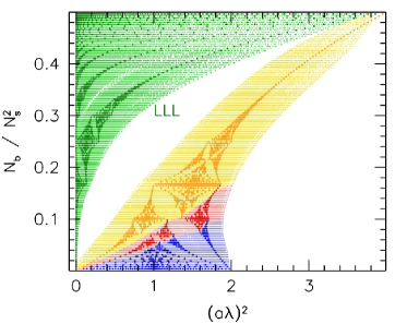
Figure 2: Lattice eigenvalues in the interacting case. In the left panel eigenmodes from a single configuration are compared to the eigenmodes in the free case. The colour code corresponds to the classification into Landau levels according to the continuum degeneracy. In the right panel, the gap between the LLL and the HLLs in physical units is shown for various lattice spacings (corresponding to the different colours) in the interacting case.

We then switch on non-Abelian interactions, in practice by taking a 2D spatial slice of a typical four-dimensional QCD configuration (for 2+1 dynamical flavours with physical masses at $T\approx 400\,{\rm MeV}$). This results into the butterfly being smeared out and the gaps disappearing, with a notable exception: the lowest group of eigenvalues remains clearly separated from the rest even in the presence of colour interactions (see Fig. 2, left panel). Moreover, the number of eigenvalues in this group matches precisely those of the continuum LLL. These features are not lattice artefacts: they survive as the lattice is made finer and finer, if the appropriate units are used, namely if eigenvalues are divided by the bare quark mass (see Fig. 2, right panel). The notion of a LLL can then be defined without ambiguity on the lattice also in the interacting case. For brevity, higher modes will be collectively labelled as higher Landau levels (HLLs), even though such higher levels do not exist individually.

3.1 Lowest Landau level and topology

The reason behind the survival of the LLL in 2D in the presence of non-Abelian fields is its topological origin, which makes it robust under (relatively) small deformations. In 2D the index theorem reads $Q^{\rm 2D}_{\rm top}=N_{\uparrow}-N_{\downarrow}$, with $Q^{\rm 2D}_{\rm top}$ the topological charge and $N_{\uparrow},N_{\downarrow}$ the number of zero modes with spin-up and spin-down polarisation in the direction of the magnetic field. Here the topological charge is just the magnetic flux (even in the presence of non-Abelian interactions),

$$Q^{\rm 2D}_{\rm top}=\frac{1}{2\pi}\int d^{2}x\,F_{xy}=\frac{1}{2\pi}\,L^{2}\cdot qB=N_{b}\,.$$ (3)

Moreover, the “vanishing theorem” Kiskis:1977vh ; Nielsen:1977aw ; Ansourian:1977qe entails that $N_{\uparrow}\cdot N_{\downarrow}=0$, and so for $qB>0$ there are exactly $N_{b}$ spin-up zero modes: these are precisely the LLL modes in the continuum (for each colour). Notice that these are the only modes with well-defined spin. When switching on non-Abelian interactions, LLL modes survive as they are protected by topology, while HLL modes mix and the corresponding structure is washed away.

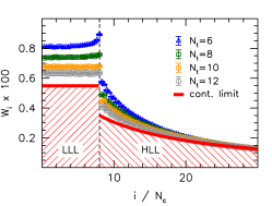
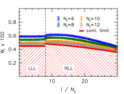
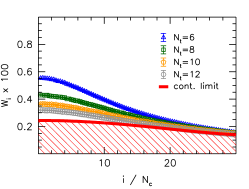
Figure 3: The overlap Eq. (7) of 4D eigenmodes with the 2D modes as a function of the 2D index (in units of $N_{c}=3$) for a magnetic flux quantum $N_{b}=8$, on configurations generated at $T\approx 400\textmd{ MeV}$. Left panel: low-lying 4D modes (with eigenvalue $220<\lambda/m<225$). Central panel: bulk 4D modes ($535<\lambda/m<545$). Right panel: same 4D modes as in the left panel, but overlap on 2D modes at $N_{b}=0$.

For staggered fermions the LLL modes are not exact zero modes, but are expected to be (and indeed are) well separated from the HLL eigenvalues. The identification of these near-zero modes as LLL modes is further supported by the finding that the matrix elements of the spin operator $\sigma_{xy}=\sigma_{z}$ are almost perfectly diagonal, and considerably different from zero only for the near-zero, LLL modes.

4 Landau levels on the lattice: four-dimensional case

In four dimensions the LLs cannot be identified by looking at the spectrum even in the free continuum case, as the contribution of the $t$ and $z$ momenta make them overlap with each other. This is however not a major obstacle: the eigenmodes $\tilde{\psi}^{(j)}_{p_{z}p_{t}}$ are in fact factorised,

$$\tilde{\psi}^{(j)}_{p_{z}p_{t}}(x,y,z,t)=\phi^{(j)}(x,y)e^{ip_{z}z}e^{ip_{t}t}\,,$$ (4)

with $\phi^{(j)}$ a solution of the 2D Dirac equation, and so one can define a projector on the LLL (or on the other levels, if so desired) and extract its contribution to any observable:

$$P =\sum_{j\leavevmode\nobreak\ \in\leavevmode\nobreak\ {\rm LLL}}\sum_{p_{z},p_{t}}\tilde{\psi}^{(j)}_{p_{z}p_{t}}\tilde{\psi}^{(j){\dagger}}_{p_{z}p_{t}}=\sum_{j\leavevmode\nobreak\ \in\leavevmode\nobreak\ {\rm LLL}}\phi^{(j)}\phi^{(j){\dagger}}\otimes\mathbf{1}_{z}\otimes\mathbf{1}_{t}=\sum_{j\leavevmode\nobreak\ \in\leavevmode\nobreak\ {\rm LLL}}\sum_{z,t}\psi^{(j)}_{zt}\psi^{(j){\dagger}}_{zt}\,.$$ (5)

In the last passage we have recast the projector as a sum over modes localised on $x,y$ slices at fixed $z,t$, namely $\psi^{(j)}_{z_{0}t_{0}}(x,y,z,t)=\phi^{(j)}(x,y)\delta_{zz_{0}}\delta_{tt_{0}}$. This construction carries over unchanged to the free lattice case, provided the appropriate extra degeneracy of staggered fermions is taken into account. Moreover, the formulation in terms of slice-localised states can be exported with little modification to the interacting case. In fact, as we have seen in the previous section, the LLL can be defined on 2D slices even in the interacting case. If we now denote with $\psi^{(j)}_{z_{0}t_{0}}$ the solutions of the 2D Dirac equation on the $x,y$ slice at $z=z_{0}$ and $t=t_{0}$ including the non-Abelian fields, the projector $P$ extracts precisely the contribution of the LLLs on all the slices to the desired observable. Ordering the 2D modes according to their eigenvalue, and taking into account the appropriate doubling and colour factors we find for staggered fermions on the lattice in the interacting case

$$P(B)=\sum_{j=1}^{2N_{c}N_{b}}\sum_{z,t}\psi^{(j)}_{zt}(B)\psi^{(j){\dagger}}_{zt}(B)\,,$$ (6)

where we have made explicit the dependence on the magnetic field. Our procedure consists essentially in changing basis from the usual localised basis, where basis vectors are localised on the lattice sites, to a new basis where the basis vectors are localised on an $x,y$ slice at fixed $z,t$, and solve the 2D Dirac equation on that slice, and then extract the LLL contribution to observables by projecting on the union of the modes corresponding to the 2D LLLs.

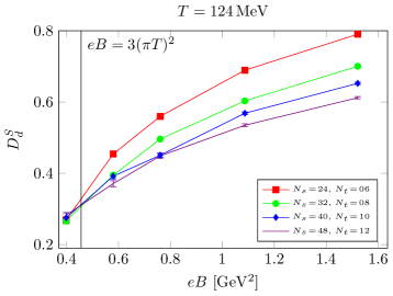
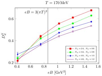
Figure 4: The ratio $D^{S}_{d}$ of Eq. (11) for the $d$ quark as a function of the magnetic field at temperatures below $T_{c}$ (left panel) and above $T_{c}$ (right panel).

If the 2D LLLs have any physical effect we should be able to see some distinctive feature in the overlap $\psi^{(i){\dagger}}_{zt}\phi$ between the solutions $\phi$ of the 4D Dirac equation and the 2D LLL modes defined on the slices. Summing over slices and 2D doublers, we define the overlap factor as

$$W_{i}(\phi)=\sum_{\rm doublers}\sum_{z,t}\big{|}\psi^{(i){\dagger}}_{zt}\phi\big{|}^{2}\,.$$ (7)

In Fig. 3 we show $W_{i}(\phi)$ after averaging over a small spectral interval of the 4D Dirac operator and over gauge configurations. The overlap of low 4D modes with the LLL modes is almost independent of the 2D mode index, and jumps abruptly downwards at the end of the LLL; in contrast, in the $B=0$ case this quantity is just continuous and monotonically decreasing. For bulk modes the jump turns upwards, but the flatness in the LLL remains. All modes turn out to have an LLL component, which is bigger for low modes. Notice that the overlap with 2D modes seems to have a finite continuum limit.

5 LLL approximation for the quark condensate

Having defined the LLL in the 4D interacting case we can now return to our main problem, and measure its contribution to the quark condensate. We have already answered (mostly negatively) the question whether the LL structure survives the introduction of colour interactions, but since the LLL survives it is still possible that it is indeed mostly responsible for MC. The LLL contribution to the condensate is simply obtained by projecting the Dirac operator on the LLL. Denoting with $\langle\ldots\rangle_{B}$ the average over gauge configurations in the presence of an external magnetic field, the full and the projected condensates read

$$\langle\bar{\psi}\psi\rangle_{B}=\langle{\rm Tr}D^{-1}_{\rm stag}\rangle_{B}\,,\qquad\langle\bar{\psi}\psi^{\rm LLL}\rangle_{B}=\langle{\rm Tr}\,PD_{\rm stag}^{-1}P\rangle_{B}\,.$$ (8)

However, both the full and the projected condensate are affected by UV divergences, and they have to be renormalised. For the full condensate it is known that the change in the condensate due to a magnetic field, $\Delta\langle\bar{\psi}\psi\rangle(B)=\langle\bar{\psi}\psi\rangle_{B}-\langle\bar{\psi}\psi\rangle_{B=0}$, is free from additive divergences. On the other hand, subtracting the LLL projected condensate at $B=0$ from that at nonzero $B$ cannot cure the analogous problem, since at $B=0$ the LLL is empty and $\langle\bar{\psi}\psi^{\rm LLL}\rangle_{B=0}=0$ identically. Instead, we notice that from the 2D perspective the change in the full condensate corresponds to the change in the contribution from all the 2D modes on all slices. Its analogue in the projected case is thus the change in the contribution of the first $2N_{c}N_{b}$ 2D modes on all slices from zero to nonzero $B$, measuring the change in the condensate due to the change in the nature of the modes which end up forming the LLL. Defining the new projector

$$\widetilde{P}(B)=\sum_{j=1}^{2N_{c}N_{b}}\sum_{z,t}\psi^{(j)}_{zt}(0)\psi^{(j){\dagger}}_{zt}(0)\,,$$ (9)

which is $B$-dependent due to the upper limit in the sum, the subtracted LLL-projected condensate is defined as

$$\Delta\langle\bar{\psi}\psi^{\rm LLL}\rangle(B)=\langle\bar{\psi}P(B)\psi\rangle_{B}-\langle\bar{\psi}\widetilde{P}(B)\psi\rangle_{0}\,.$$ (10)

It can be shown explicitly that this quantity is indeed free of additive divergences in the free case. Since the additive divergence comes from the large 4D modes where the SU$(3)$ interaction is negligible, we expect that $\Delta\langle\bar{\psi}\psi^{\rm LLL}\rangle(B)$ be free of additive divergences also in the interacting case.

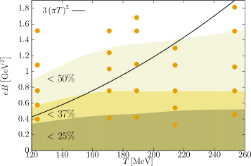
Figure 5: Visualisation of the validity of the LLL-approximation for the $d$ quark condensate. The lighter the color, the closer the LLL-projected condensate is to the full result. The orange dots denote our simulation points and the solid black line marks $|q_{d}B|=(\pi T)^{2}$.

The multiplicative divergence can be studied by means of a spectral decomposition of the projected condensate. If the overlap of 4D modes with the LLL, averaged over configurations and small (infinitesimal) spectral intervals, has a continuum limit throughout the spectrum both at zero and finite $B$, then the multiplicative divergence is the same as in the full condensate, and therefore cancels in ratios. The plots in Fig. 3 indeed support the existence of a continuum limit for the overlap. Nonetheless, such a delicate issue requires more detailed studies than the present one, and for this reason the continuum limit is not taken in this work.

Independently of the issue of renormalisability, the ratio of the projected and full condensates after subtracting their additive divergences,

$$D^{S}=\frac{\Delta\langle\bar{\psi}\psi^{\rm LLL}\rangle(B)}{\Delta\langle\bar{\psi}\psi\rangle(B)}=\frac{\langle\bar{\psi}P(B)\psi\rangle_{B}-\langle\bar{\psi}\widetilde{P}(B)\psi\rangle_{0}}{\langle\bar{\psi}\psi\rangle_{B}-\langle\bar{\psi}\psi\rangle_{0}}\,,$$ (11)

measures how much of the change of the condensate is due to the LLL at a given lattice spacing. If this ratio is divergence-free, then it has full physical meaning, and it measures the physical contribution of the LLL to the change of the condensate. By measuring it we can therefore answer our question about the role of the LLL in the valence effect. If the LLL dominates the (change in the) condensate, then this would naturally provide an explanation for the valence effect (and thus for MC) as a consequence of the increased degeneracy of the LLL. If the LLL does indeed dominate the condensate, it is expected to do so on a configuration-by-configuration basis, and therefore it should not matter, at least from the qualitative point of view, whether we include the magnetic field in the fermionic determinant or not: this would just lead to a reweighting of the configurations. For this reason, we decided to simplify our problem and consider only the valence effect of the magnetic field, i.e., we included it in the observables but not in the fermionic determinant. This should be enough to decide whether the condensate is dominated by the LLL or not.

In Fig. 4 we show the results for $D^{S}$ at two temperatures, one below and one above $T_{c}$, obtained for the $d$ quark condensate ($q_{d}=-\frac{e}{3}$) in our numerical simulations of 2+1 flavours of improved rooted staggered fermions (see Ref. Bali:2011qj for technical details). The $B$ field was not included in the fermionic determinant. We show results for various magnetic fields and different lattice spacings $a=1/(N_{t}T)$, where $N_{t}$ is the temporal extension of the lattice in lattice units. The ratio $D^{S}_{d}$ seems to show a nice scaling towards the continuum limit; increases with $B$, slowly approaching 1, as one expects; and decreases with $T$. The results of all our simulations are summarised in Fig. 5, where we show the regions of the $T-B$ plane where the change in the projected condensate reaches a given fraction of the change in the full condensate. This is estimated using our finest lattices, which, given the trend shown in Fig. 4, probably overestimates this fraction. This allows to answer our question whether the LLL dominates or not the change in the condensate: except for very large magnetic fields ($eB\sim 1\div 1.5\,{\rm GeV}^{2}$) the LLL is responsible for less than 50% of the change in the condensate.

6 Conclusions

In this work we studied the issue of Landau levels on the lattice and investigated the validity of the lowest-Landau-level (LLL) approximation to QCD in the presence of background magnetic fields. The presence of (nonperturbative) color interactions mixes the levels, washing away the Landau level structure, with the exception of the LLL. This can be defined in a consistent manner even for strongly interacting quarks, thanks to a two-dimensional topological argument that characterises the plane perpendicular to the magnetic field. This allows to define a projector on the LLL that can be used to extract its contribution to the observables. Observables in 4D are sensitive to the LLL, and in particular a sizeable fraction of the change in the quark condensate comes from it. On the other hand, the LLL does not dominate this change except for very large magnetic fields, i.e., the LLL approximation typically underestimates the change in the condensate. In other words, the LLL alone cannot fully explain the valence effect and MC in most of the $T-B$ plane.

References

- (1) D. Kharzeev, K. Landsteiner, A. Schmitt, H.U. Yee, Lect. Notes Phys. 871, 1 (2013)
- (2) V.A. Miransky, I.A. Shovkovy, Phys. Rept. 576, 1 (2015), 1503.00732
- (3) G.S. Bali, F. Bruckmann, G. Endrődi, Z. Fodor, S.D. Katz, S. Krieg, A. Schäfer, K.K. Szabó, JHEP 02, 044 (2012), 1111.4956
- (4) M. D’Elia, S. Mukherjee, F. Sanfilippo, Phys. Rev. D82, 051501 (2010), 1005.5365
- (5) F. Bruckmann, G. Endrődi, T.G. Kovács, JHEP 04, 112 (2013), 1303.3972
- (6) I.A. Shovkovy, Lect. Notes Phys. 871, 13 (2013), 1207.5081
- (7) J.O. Andersen, W.R. Naylor, A. Tranberg, Rev. Mod. Phys. 88, 025001 (2016), 1411.7176
- (8) C.N. Leung, S.Y. Wang, Annals Phys. 322, 701 (2007), hep-ph/0503298
- (9) S. Fayazbakhsh, N. Sadooghi, Phys. Rev. D82, 045010 (2010), 1005.5022
- (10) K. Fukushima, Phys. Rev. D83, 111501 (2011), 1103.4430
- (11) E.J. Ferrer, V. de la Incera, I. Portillo, M. Quiroz, Phys. Rev. D89, 085034 (2014), 1311.3400
- (12) F. Bruckmann, G. Endrődi, M. Giordano, S.D. Katz, T.G. Kovács, F. Pittler, J. Wellnhofer, Phys. Rev. D96, 074506 (2017), 1705.10210
- (13) D.R. Hofstadter, Phys. Rev. B14, 2239 (1976)
- (14) G. Endrődi, PoS LATTICE2014, 018 (2014), 1410.8028
- (15) J.E. Kiskis, Phys. Rev. D15, 2329 (1977)
- (16) N.K. Nielsen, B. Schroer, Nucl. Phys. B127, 493 (1977)
- (17) M.M. Ansourian, Phys. Lett. B70, 301 (1977)
- (18) R. Bignell, D. Leinweber, W. Kamleh, M. Burkardt, PoS INPC2016, 287 (2017), 1704.08435