On Minimal Dark Matter coupled to the Higgs

Abstract

We provide a unified presentation of extensions of the Minimal Dark Matter framework in which new fermionic electroweak multiplets are coupled to each other via the Standard Model Higgs doublet. We study systematically the generic features of all the possibilities, starting with a singlet and two doublets (akin to Bino-Higgsino dark matter) up to a Majorana quintuplet coupled to two Weyl quadruplets. We pay special attention to this last case, since it has not yet been discussed in the literature. We estimate the parameter space for viable dark matter candidates. This includes an estimate for the mass of a quasi-pure quadruplet dark matter candidate taking into account the Sommerfeld effect. We also argue how the coupling to the Higgs can bring the Minimal Dark Matter scenario within the reach of present and future direct detection experiments.

1 Introduction

The Minimal Dark Matter (MDM) Cirelli:2005uq ; Cirelli:2009uv scenario is one of the simplest extensions of the Standard Model with a dark matter (DM) candidate. It requires the addition of one single (real or complex) scalar or (Majorana or Dirac) fermionic $SU(2)_{L}$ multiplet, with mass $M$ as the only free parameter. A mass splitting between the components of the multiplet arises as a loop correction and it is a generic outcome that the lightest component is neutral and thus a potential dark matter candidate. Such a candidate is a WIMP (indeed a perfect WIMP, or WIMP archetype, as it has only electroweak interactions) and matching with the observed DM abundance points to a specific prediction for the mass $M$ of the thermal candidate, different for each representation, but all in the TeV range. The precise determination of this mass is however notoriously delicate because of non-perturbative effects that must be taken into account to calculate the effective annihilation cross section of the DM in the early Universe, a point to which we shall come back. The classification of possible $SU(2)_{L}$ representations may be further restricted by requiring the absence of a Landau pole, potentially up to the Planck scale. For a fermion (scalar) candidate, the largest admissible representation is in a quintuplet (respectively septuplet) of $SU(2)_{L}$. Interestingly the stability of DM may be automatic in the case of a quintuplet (in the sense that the lifetime of the DM candidate is naturally long, even taking into account the possible contribution from effective operators), without the need to impose an ad hoc discrete $Z_{2}$ symmetry Cirelli:2005uq (a scalar septuplet however, despite being in a large representation of $SU(2)_{L}$, may be unstable at one-loop DiLuzio:2015oha ). For this reason, depending on the context or on the authors, Minimal Dark Matter may refer to the quintuplet candidate only, or the whole set of admissible electroweak multiplets; we will adopt the latter definition.

Minimal Dark Matter candidates, like potentially any WIMP, may be searched experimentally. Most relevant for MDM are constraints from indirect and direct searches (assuming that MDM is the dominant form of DM within a standard cosmological evolution). First, direct detection limits exclude any MDM candidate with non-zero hypercharge (hence a Dirac fermion or a complex scalar) due to scattering off nucleons through $Z$ boson exchange. Now, sufficient mass spitting between the neutral components can help to alleviate such constraints, see e.g. DeSimone:2010tf . This is what we will assume when quoting doublet and quadruplet cross-sections below. For a Majorana or real scalar candidate, a coupling to nucleons arises at one-loop (with only a spin-independent (SI) contribution in the scalar case), see e.g. Cirelli:2005uq for a first estimation. The scattering cross-section of MDM off nucleons has been carefully revisited at NLO in ref. Hisano:2015rsa and, for a fermion MDM-proton scattering, in a representation of dimension $n$ and of hypercharge $Y$, one has:

$$\sigma_{\rm SI}=\frac{4}{\pi}\mu^{2}f_{p}^{2}\quad{\rm with}\quad f_{p}=(n^{2}-4Y^{2}-1)f^{W}_{p}+Y^{2}f^{Z}_{p}$$ (1)

with $f_{p}^{W}=2.9\,10^{-10}$ GeV^-2 and $f_{p}^{Z}=-1.8\,10^{-10}$ GeV^-2 and $\mu=m_{DM}m_{p}/(m_{DM}+m_{p})$ is the reduced mass. Such estimation gives rise to lower cross-sections than originally estimated and appear to be above the neutrino floor (except for the doublet) and potentially marginally testable by the Xenon 1T Aprile:2015uzo experiment. In particular, from eq. (1), one gets $\sigma_{\rm SI}=8.4\times 10^{-50}$ cm² for a fermion doublet, with $(n,Y)=(2,1/2)$, $\sigma_{\rm SI}=2.7\times 10^{-47}$ cm² for a triplet (or 3-plet for short), with $(n,Y)=(3,0)$, $\sigma_{\rm SI}=1.6\times 10^{-46}$ cm² for a quadruplet (4-plet), with $(n,Y)=(4,1/2)$, and finally, $\sigma_{\rm SI}=2.4\times 10^{-46}$ cm² for a quintuplet (5-plet), with $(n,Y)=(5,0)$. Notice that in all cases, one can also compute the spin-dependent scattering on nucleons. We have checked that, at tree-level, the spin-dependent scattering cross-sections are way beyond current DM searches limits (for a recent analysis, see e.g. Hill:2014yxa ).

Indirect detection limits on MDM candidates are also strong, at least assuming an Einasto or Navarro-Frenk-White (NFW) profiles for the dark matter distribution in the Galaxy. This is because of the Sommerfeld effect, which typically enhances the annihilation cross section of MDM candidates at small relative velocities, giving rise to strong gamma-ray spectral features, see Lefranc:2016fgn ; Ovanesyan:2014fwa ; Baumgart:2014saa for the wino case and Cirelli:2015bda ; Garcia-Cely:2015dda for the quintuplet. Notice that on general grounds, dark matter bound state formation MarchRussell:2008tu ; Ellis:2015vaaw ; vonHarling:2014kha ; Wise:2014jva ; Liew:2016hqo could also affect the dark matter annihilation. It has been shown that the latter effect is expected to be relevant for quintuplet dark matter, while it is negligible in the case of the triplet Asadi:2016ybp ; Mitridate:2017izz . In general, the wino-like dark matter appears now strongly disfavoured by current indirect detection searches Ovanesyan:2016vkk while the quintuplet could be tested by very near future HESS-II data release on searches for gamma-ray lines from the 10 years Galactic Center data HESStalk .

Because of the advent of these constraints, it may be timely to consider possible variations around the MDM framework, which at the same time may lead to a broader range of possible DM candidates. As mentioned above, a basic assumption of this framework is that there is one and only one electroweak multiplet. This, in particular, precludes Yukawa coupling to the SM Higgs doublet for fermionic candidates. A natural yet simple variation on the MDM framework is to consider simultaneously different multiplets, in particular fermionic representations that differ by isospin $\Delta I=1/2$, that allows for “integrating the Higgs portal to fermion DM” Freitas:2015hsa . A familiar instance is the neutralino of the Minimal Supersymmetric Standard Model (MSSM), which is generically a mixture of bino/higgsino/wino complex. Recently, there have been much studies of DM candidates from mixed (as compared to pure) representations: singlet-doublet ($\sim$ bino-higgsino) Mahbubani:2005pt ; D'Eramo:2007ga ; Enberg:2007rp ; Cohen:2011ec ; Cheung:2013dua ; Calibbi:2015nha ; Banerjee:2016hsk ; Freitas:2015hsa (see also Yaguna:2015mva for the case of a Dirac singlet), doublet-triplet ($\sim$ higgsino-wino) Beneke:2016jpw ; Freitas:2015hsa ; Dedes:2014hga and triplet-quadruplet Tait:2016qbg ; Banerjee:2016hsk .

In the present work, we complete this panorama by adding to this list the case of two Weyl 4plets coupled to a Majorana 5-plet (thus called $5_{M}4_{D}$), while discussing in an unified manner the rest of the HMDM candidates. This may be of particular interest given the special status of the fermionic 5-plet within the MDM framework, as alluded to above. The scenarios that we consider rest on only 4 free parameters: 2 bare masses (one Dirac mass, $m_{D}$, and one Majorana mass, $m_{M}$), and two Yukawa couplings to the Higgs, $y_{1}$ and $y_{2}$ hence 3 extra parameters compared to the pure MDM case (in the sequel, we will refer to pure, i.e. à la MDM, and mixed states). Considering thermal candidates leaves a 3-dimensional subspace of possible candidates to explore. The goal of this paper is to illustrate that, due to the Yukawa coupling to the Higgs, Higgs coupled MDM (denoted HMDM in what follows) scenarios allow to enlarge the DM mass range of pure MDM scenarios in a controlled way, and to argue that they could potentially allow to evade current indirect detection constraints while providing the opportunity to give rise to a signal in near future direct detection facilities.

The structure of the paper is as follows. We begin this article describing the general properties of HMDM in a unified framework and analyze the properties of the mass spectra of both neutral and charged states in Sec. 2. We then discuss the viable parameter space for a HMDM dark matter candidate taking into account non perturbative corrections to the processes of (co)-annihilation making use of the SU(2)_L symmetric limit and discuss briefly the prospects for dark matter detection in Sec. 3. We finally conclude in Sec. 4 and provide some extra material in the appendix.

2 Higgs coupled Minimal Dark Matter (HMDM)

We consider left-handed Weyl fermions, $\psi$ and $\tilde{\psi}$, in a $2n$-dimensional representation of $SU(2)_{L}$ with hypercharge $Y_{\psi}=-Y_{\tilde{\psi}}=1/2$ (i.e. an anomaly free, vector-like fermion), together with a Majorana fermion, $\chi$, (hence with $Y_{\chi}=0$) in a $2n\pm 1$ representation of $SU(2)_{L}$. Going to 4-components notation, one can construct the Dirac fermion $2n$-plet as $\Psi=(\psi,\epsilon\tilde{\psi}^{\dagger})$, with ($\epsilon=i\sigma_{2}$ the anti-symmetric tensor of SU(2)) and $X=(\chi,\epsilon\chi^{\dagger})$ the Majorana fermion. As mentioned in the introduction, the fermions quantum numbers are chosen so that these fields may have a Yukawa coupling to the SM Higgs and contain a neutral particle. To ensure DM stability, we assume that all fields of the dark sector are odd under a $Z_{2}$ symmetry, while the Standard Model particles are even.

M\D	2	4	6
1	✓ Mahbubani:2005pt ; D'Eramo:2007ga ; Enberg:2007rp ; Cohen:2011ec ; Cheung:2013dua ; Calibbi:2015nha ; Banerjee:2016hsk ; Freitas:2015hsa
3	✓ Beneke:2016jpw ; Freitas:2015hsa ; Dedes:2014hga	✓ Tait:2016qbg ; Banerjee:2016hsk
5		✓	✓
7			✓

Table 1: The HMDM Model Space. Check marks correspond to pairs of Dirac (D) and Majorana (M) DM representations that can have a Yukawa coupling to the SM Higgs. The green cells are models with a Landau pole (LP) for $\alpha_{2}$ at $\Lambda_{\rm LP}\geq M_{Pl}$, while the yellow, orange and red cells correspond to $\Lambda_{\rm LP}$ in $[M_{Pl},10^{10}{\rm GeV}]$, $[10^{10}{\rm GeV},10^{5}{\rm GeV}]$ and $<10^{5}$ GeV respectively.

As in the usual MDM framework, we may require that the DM sector does not drive electroweak couplings to a Landau pole at a too low energy scale. This requirement sets upper limits on the possible pairs of Dirac (noted $D$) and Majorana (resp. $M$) $SU(2)_{L}$ representations that are stronger than for pure MDM candidates. This leads to the results summarized in Table 2, where we show the $D/M$ pairs with, respectively, no Landau pole below $\Lambda_{\rm LP}=M_{\rm Pl}$ (green cells), $\Lambda_{\rm LP}=10^{10}\,$GeV (yellow cells) and $\Lambda_{\rm LP}=100\,$TeV (orange cells). The red cells correspond to representations that have a Landau pole below $100\,$TeV. In this work, we will consider that models with no Landau pole below $10^{10}$ GeV are acceptable, which leaves some room for other, heavier degrees of freedom to address the Landau pole problem.

2.1 Lagrangian

The generic form of the Lagrangian we consider is

$${\cal L}\supset-m_{D}\psi\tilde{\psi}-{1\over 2}m_{M}\chi\chi-y_{1}\psi\chi H^{*}-y_{2}\tilde{\psi}\chi H+\mbox{\rm h.c.}$$ (2)

together with the kinetic terms of the new degrees of freedom. We take the Yukawa couplings to be real. We use the $SU(2)$ tensor formalism so that appropriate contractions of indices are assumed. It may be useful to explicitly discuss a few examples. Writing the components of the Higgs doublet as $H=(\phi^{+},\phi^{0})^{T}$, the simplest case is the Yukawa coupling of two Weyl doublets, $\psi_{i}$ and $\tilde{\psi}_{i}$ with $i=1,2$, and one Majorana singlet $\chi$ or Bino-Higgsino system, to which we will refer as $1_{M}2_{D}$,

$$-y_{1}\chi\psi_{i}H^{*i}=-y_{1}(\phi^{0*}\chi^{0}\psi^{0}+\phi^{+*}\chi^{0}\psi^{+})\,,$$

$$-y_{2}\chi\tilde{\psi}_{i}H_{j}\epsilon^{ij}=-y_{2}(\phi^{0}\chi^{0}\tilde{\psi}^{0}-\phi^{+}\chi^{0}\tilde{\psi}^{-})\,.$$ (3)

The next instance is the doublet-triplet system (i.e. Wino-Higgsino) or $3_{M}2_{D}$. The Weyl fermions are as above, while the Majorana triplet is represented by an $SU(2)_{L}$ symmetric tensor with 2 indices, $\chi_{ij}=\chi_{ji}$. The correspondence between the tensor basis and the more familiar basis in terms of eigenmodes of the $T_{3}$ generators ($T_{3}$ basis below) is easy to work out. For the $3_{M}$ we have

$$\left(\!\begin{array}[]{c}\chi_{11}\\ \sqrt{2}\chi_{12}\\ \chi_{22}\end{array}\!\!\!\right)\equiv\left(\!\begin{array}[]{c}\chi^{+}\\ \chi^{0}\\ \chi^{-}\end{array}\!\right)\,,$$ (4)

and the Yukawa couplings then take the form

$$-y_{1}\psi_{i}\chi_{i^{\prime}j}H^{*j}\epsilon^{i^{\prime}i}=-y_{1}({1\over\sqrt{2}}\phi^{0*}\chi^{0}\psi^{0}-\phi^{0*}\chi^{-}\psi^{+}+\phi^{+*}\chi^{+}\psi^{0}-{1\over\sqrt{2}}\phi^{+*}\chi^{0}\psi^{+})\,,$$

$$-y_{2}\tilde{\psi}_{i}\chi_{i^{\prime}j}H_{j^{\prime}}\epsilon^{ii^{\prime}}\epsilon^{jj^{\prime}}=-y_{2}({1\over\sqrt{2}}\phi^{+}\chi^{0}\tilde{\psi}^{-}-\phi^{+}\chi^{-}\tilde{\psi}^{0}+{1\over\sqrt{2}}\phi^{0}\chi^{0}\tilde{\psi}^{0}-\phi^{0}\chi^{+}\tilde{\psi}^{-})\,.$$

The other cases are compiled in Appendix A.

The above combination of bare masses and Yukawa couplings gives rise to mass matrices $M_{Q}$ for a set of fermions of charge $Q=T_{3}+Y$ that take the same form for all the models studied here and are uniquely determined by group representation. In e.g. the basis $\{\chi^{Q},\psi^{Q},\tilde{\psi}^{Q}\}$, in the cases where 3 fermions appear to have the same charge $Q$, $M_{Q}$ is given by:

$$M_{Q}^{3\times 3}\!=\!(-1)^{Q}\left(\!\!\begin{array}[]{ccc}m_{M}&a_{Q}\hat{m}_{1}&\tilde{a}_{Q}\hat{m}_{2}\\ \tilde{a}_{Q}\hat{m}_{1}&0&m_{D}\\ a_{Q}\hat{m}_{2}&m_{D}&0\end{array}\!\!\right)\,,$$ (5)

while for one or two states of charge $Q$, $M_{Q}$ take the form:

$$M_{Q}^{2\times 2}\!=\!(-1)^{Q}\left(\!\!\begin{array}[]{cc}m_{M}&\hat{m}_{1}\\ \hat{m}_{2}&m_{D}\\ \end{array}\!\!\right)\,,\quad M_{Q}^{1\times 1}\!=\!(-1)^{Q}m_{D}\,,$$ (6)

with $\hat{m}_{1,2}=y_{1,2}v/\sqrt{2}$ (with $v=246\,$ GeV) and

$$a_{Q}=\textrm{min}\Big{[}{n_{\chi^{(-Q)}}\over n_{\psi^{Q}}},{n_{\psi^{Q}}\over n_{\chi^{(-Q)}}}\Big{]}\,,\quad\tilde{a}_{Q}=\textrm{min}\Big{[}{n_{\chi^{(-Q)}}\over n_{\tilde{\psi}^{Q}}},{n_{\tilde{\psi}^{Q}}\over n_{\chi^{(-Q)}}}\Big{]}\,.$$ (7)

Here the $n_{\Psi^{(\pm Q)}}$ is the normalization factor that relates a given component of a multiplet $\Psi$ of charge $\pm Q$ in the tensor basis to that in the $T_{3}$ basis, as given in Appendix A. For instance, from (4) we have for the triplet $\sqrt{2}\chi_{12}\equiv\chi^{0}$ and thus $n_{\chi^{0}}=\sqrt{2}$, while $\chi_{22}\equiv\chi^{+}$ and so $n_{\chi^{+}}=1$. For Yukawa couplings between a triplet and doublets, $a_{0}=\tilde{a}_{0}=1/\sqrt{2}$.

2.2 Mass spectra

To discuss the mass spectra we will exploit the existence of a global $SU(2)_{R}$ symmetry, that mixes $\psi$ and $\tilde{\psi}$ when $y_{1}=\pm y_{2}$, to which we will refer as custodial points (see e.g. Tait:2016qbg ). A practical interest of that symmetry is that one can have rather transparent and simple analytic expressions for the mass spectrum and mixing matrices (at least at tree level). More physically, we will see that it implies that, after EW symmetry breaking, the particles fall into multiplets of the diagonal subgroup $SU(2)\subset SU(2)_{L}\times SU(2)_{R}$. Away from $y_{1}=\pm y_{2}$, the mass eigenstates are split but, thanks to the custodial symmetry, we will see that they remain nearly degenerate and thus can still be classified in terms of $SU(2)$ multiplets.

We begin by considering the custodial limit, and then discuss in qualitative terms the more general situation. In principle we only need to consider the case $y_{1}=y_{2}$ as, through the field redefinition $\tilde{\psi}\rightarrow-\tilde{\psi}$, $y_{1}=-y_{2}$ is equivalent to $y_{1}=y_{2}$ together with a flip in sign of the Dirac mass, $m_{D}\rightarrow-m_{D}$. However, we find it more convenient to fix the sign of $m_{D}$ and let the Yukawa couplings to have arbitrary signs.

2.2.1 Neutral states

Setting $y_{1}=y_{2}=y$ the mass matrix of neutral states is diagonalized by going from the basis $\xi_{i}=\{\chi_{0},\psi_{0},\tilde{\psi}_{0}\}$ with ${\cal L}_{m}=-\frac{1}{2}\sum_{ij}M_{0,ij}\xi_{i}\xi_{j}$ to the basis $\chi_{i}=\{\chi^{0}_{1},\chi^{0}_{2},\chi^{0}_{3}\}$ with ${\cal L}_{m}=-\frac{1}{2}\sum_{i}m_{i}\chi_{i}\chi_{i}$ and

$$m_{1} = \frac{1}{2}(m_{M}+m_{D}+\Delta m_{\eta})$$

$$m_{2} = m_{D}$$ (8)

$$m_{3} = \frac{1}{2}(m_{M}+m_{D}-\Delta m_{\eta})$$

where

$$\Delta m_{\eta}=\sqrt{(m_{D}-m_{M})^{2}+8(\eta yv/\sqrt{2})^{2}}\,.$$ (9)

Notice that $\eta$ is equal to the coefficients $a_{Q=0}=a_{\tilde{Q}=0}$ that appear in the $M_{0}$ mass matrix of eq. (5). In particular, for the cases that we are interested in, we have:

$$\eta=\left\{\begin{array}[]{lllc}1&&&1_{M}2_{D}\\ {1/\sqrt{2}}&&&3_{M}2_{D}\;\&\;5_{M}4_{D}\\ \sqrt{2/3}&&&3_{M}4_{D}\end{array}\right.$$ (10)

For the diagonalisation, we use the transformation

$$\left(\!\begin{array}[]{c}\chi_{1}^{0}\\ \chi_{2}^{0}\\ \chi_{3}^{0}\end{array}\!\right)\!=\!\left(\!\!\begin{array}[]{ccc}c_{\eta}&s_{\eta}/\sqrt{2}&s_{\eta}/\sqrt{2}\\ 0&i/\sqrt{2}&-i/\sqrt{2}\\ -s_{\eta}&c_{\eta}/\sqrt{2}&c_{\eta}/\sqrt{2}\\ \end{array}\!\!\right)\!\left(\!\begin{array}[]{c}\chi_{0}\\ \psi_{0}\\ \tilde{\psi}_{0}\end{array}\!\right)$$ (11)

with $s_{\eta}=\sin\theta_{\eta}$ and $c_{\eta}=\cos\theta_{\eta}$ considering

$$\sin^{2}\theta_{\eta}=\frac{1}{2}\left(1+\frac{m_{D}-m_{M}}{\Delta m_{\eta}}\right)\,.$$ (12)

The transformation matrix used in eq. (11) is equivalent to the one of Freitas:2015hsa up to some differences in normalization and sign conventions. In addition, our $\chi^{0}_{i}$ indices $i=1,2,3$ do not point to any mass ordering. The latter depends on the hierarchies between $m_{D}$ and $m_{M}$ and between $\eta yv$ and $\sqrt{m_{D}^{2}-m_{M}m_{D}}$. Going from the basis above to the mass ordered basis $\{\chi^{0}_{\alpha}\}$ with indices $\alpha=l,m,h$ (refering to the light, medium and heavy states) just simply imply a reordering of the transformation matrix entries. The Lagrangian with couplings to the Higgs ($h$) and the Z boson takes the form

$$\cal L = -\frac{g}{2}(\psi_{0}^{\dagger}\bar{\sigma}^{\mu}\psi_{0}-\tilde{\psi}_{0}^{\dagger}\bar{\sigma}^{\mu}\tilde{\psi}_{0})Z_{\mu}-y\eta(\tilde{\psi}_{0}-\psi_{0})\chi_{0}\,h,$$ (13)

which corresponds in the basis of mass eigenstates to

$$\cal L = \frac{g}{2}\chi_{2}^{0*}\bar{\sigma}^{\mu}(s_{\eta}\chi_{1}^{0}+c_{\eta}\chi_{3}^{0})Z_{\mu}+h.c.$$ (15)

$$-\frac{y\eta}{2\sqrt{2}}\left(s_{2\eta}(\chi_{1}^{0}\chi_{1}^{0}-\chi_{3}^{0}\chi_{3}^{0})+2c_{2\eta}\chi_{1}^{0}\chi_{3}^{0}\right)\,h+h.c.$$

with $s_{2\eta}=\sin(2\theta_{\eta})$ and $c_{2\eta}=\cos(2\theta_{\eta})$. This is in agreement with Freitas:2015hsa for $1_{M}2_{D}$ and $3_{M}2_{D}$, up to distinct phase conventions.

We first briefly comment on the above Lagrangian, as it will be of interest for DM scattering on nucleons. First of all, the couplings to the $Z$ are non-diagonal reflecting the fact that, unless $y=0$, the mass eigenstates are all Majorana particles. The constraints from direct dark matter searches are thus avoided provided the mass differences between $\chi_{1,3}$ and $\chi_{2}$ are larger than ${\cal O}$(100 keV) TuckerSmith:2001hy . Notice also that one of the neutral particles (here $\chi_{2}$) does not couple to the Higgs. This feature is also generic, as only the combination $\sim y_{1}\psi+y_{2}\tilde{\psi}$ mixes with the Majorana multiplet (see also footnote 6). Then there are some potentially interesting limiting cases (see also Freitas:2015hsa ):

• From (2.2.1) and (12) we see that the Lightest Neutral Particle (LNP) has maximal coupling to the Higgs when $m_{M}\simeq m_{D}$ and $y_{1}\simeq y_{2}$ with $y_{1},y_{2}\gg|m_{M}-m_{D}|/(2\sqrt{2}\eta v)$. Indeed at the custodial point $y_{1}=y_{2}$ and $m_{N}=m_{D}$ so that $\chi_{3}^{0}=\chi_{0}$ is the DM candidate and $\theta_{\eta}=\pi/4$. Moving away from this custodial point, we have checked numerically that the coupling to the Higgs remains close to maximal coupling when $m_{M}\simeq m_{D}$, $y_{1}$ and $y_{2}$ have the same sign and $|y_{1}+y_{2}|\gg 1$.

• In the limit $m_{D}\gg m_{M}$ and $y_{1}\simeq y_{2}$ with $y_{1},y_{2}\ll|m_{M}-m_{D}|/(2\sqrt{2}\eta v)$ one recovers the case of the Majorana DM case with zero coupling to the Higgs and kinematically suppressed coupling to the $Z$. Indeed, at the custodial point $y_{1}=y_{2}$ ($y_{1}=-y_{2}$), $\chi_{3}^{0}=\chi_{0}$ (resp. $\chi_{1}^{0}=\chi_{0}$) is the DM candidate and $\theta_{\eta}=\pi/2$ (resp. $\theta_{\eta}=0$).

• When $m_{M}\gg m_{D}$ and $y_{1}\simeq y_{2}$ with small enough Yukawa couplings the states $\chi_{0}^{3}$ and $\chi_{0}^{2}$ have a mass splitting $\delta m={\cal O}(y^{2}v^{2}/m_{N})$, forming a pseudo-Dirac fermion and their coupling to the $Z$ is maximal as $\theta_{\eta}\simeq 0$. As usual, to avoid constraints from direct detection, the mass splitting must satisfy $\delta m>{1/2}\mu v^{2}\sim 100$ keV, where $v\simeq 10^{-3}$ is the velocity of the dark matter and $\mu$ is the reduced mass of the dark matter/direct detection target nucleus TuckerSmith:2001hy , see Sec. 3.3.1 for more details.

• Finally, let us stress that for $m_{M}\simeq m_{D}$ but $y_{1}\simeq-y_{2}$, i.e. with Yukawas of opposite signs, the lightest neutral state has suppressed coupling to the Higgs. This can be seen from Eqs. (2.2.1) and (12), obtained in the limit $y_{1}=y_{2}=y$, by setting $m_{D}\rightarrow-m_{D}$. In the latter case, the LNP is $\chi_{2}^{0}$ and corresponds to the combination of Weyl states $\propto\psi_{0}-\tilde{\psi}_{0}$ that does not couple to the Higgs. As one departs from this custodial point, the LNP mixes with the neutral component of the Majorana multiplet, $\chi_{0}$, and so couples to the Higgs. We have checked numerically that this behavior holds over a broad range of parameters away from the custodial point $y_{1}=-y_{2}$.

2.2.2 Charged states and $SU(2)$ multiplets structure

We now comment on the mass spectrum of the charged partners. As mentioned above, at the custodial points the neutral, singly charged and, if present, doubly charged eigenstates combine into multiplets of the custodial $SU(2)$. Of course, the custodial symmetry is only approximate, being explicitly broken by coupling to $U(1)_{Y}$ gauge bosons. In the case of Minimal Dark Matter, one-loop electroweak corrections induce splittings ${\cal O}$(100 MeV) between the components of a multiplet such that the neutral state of a multiplet with $Y=0$ is always the lightest component, and so is potentially a dark matter candidate Cirelli:2005uq , see also McKay:2017rjs for a recent discussion. Once non-zero Yukawa couplings between different representations are considered, there are more possibilities as, away from the custodial points, mass splittings between components are obtained already at tree level. We first focus on tree-level splittings and then comment on the potential effects of loop corrections.

A first feature is that for $y_{1}=\pm y_{2}$, the Majorana and two Weyl states mix and, together, neutral and charged particles combine to form Majorana $SU(2)$ multiplets according to the following pattern:

$$1_{M}2_{W}2_{W}\rightarrow 1_{M}1_{M}3_{M} 3_{M}2_{W}2_{W}\rightarrow 3_{M}1_{M}3_{M}$$

$$3_{M}4_{W}4_{W}\rightarrow 3_{M}3_{M}5_{M} 5_{M}4_{W}4_{W}\rightarrow 5_{M}3_{M}5_{M}\,.$$

In essence, the two n-plet Weyl states (of same chirality and thus opposite hypercharge) combine to form a Majorana $(n+1)$-plet, the orthogonal state being a Majorana $(n-1)$-plet. At the custodial points, the components of each multiplet are degenerate, but distinct multiplets have a distinct mass. The multiplet that contains the dark matter candidate can be determined by direct evaluation of the mass eigenstates. However, as the mixing between three neutral states involves solving a cubic equation, the outcome is not a priori obvious. Fortunately, the mass spectra have some general features, which are easy to grasp using the custodial symmetry.

In what follows, we provide a detailed case by case study. In essence, the relevant points of the discussion below can be summarized as follows: 1) at the custodial points, the LNP belongs in general (it can be in a $1_{M}$, for instance in the $1_{M}2_{D}$) to a multiplet of the $SU(2)$ custodial symmetry; 2) away from the custodial points, the multiplet components are split, but the splitting is somewhat protected by the custodial symmetry and 3) the LNP is always the lightest component of the multiplet; 4) the mass splitting are ${\cal O}((y_{1}\pm y_{2})^{2}v^{2}/m_{M})$ if $m_{M}\gg m_{D}$ and ${\cal O}((y_{1}^{2}-y_{2}^{2})v^{4}/m_{D}^{3})$ if $m_{M}\ll m_{D}$, assuming small Yukawa couplings.

M-D system	$m_{M}<m_{\ast}\sim m_{D}$	$m_{M}>m_{\ast}\sim m_{D}$
$1_{M}2_{D}\sim 1_{M}1_{M}3_{M}$	$\chi_{l}^{0}\sim 1_{M}$	$\chi_{l}^{0}\subset\left\{\begin{array}[]{lll}3_{M}&{\rm at}&y_{1}=-y_{2}\\ 1_{M}&{\rm at}&y_{1}=y_{2}\end{array}\right.$
$3_{M}2_{D}\sim 1_{M}3_{M}3_{M}$	$\chi_{l}^{0}\subset 3_{M}$	$\begin{array}[]{lll}1_{M}&&y_{1}=-y_{2}\\ 3_{M}&&y_{1}=y_{2}\end{array}$
$3_{M}4_{D}\sim 3_{M}3_{M}5_{M}$	$3_{M}$	$\begin{array}[]{lll}5_{M}&&y_{1}=-y_{2}\\ 3_{M}&&y_{1}=y_{2}\end{array}$
$5_{M}4_{D}\sim 3_{M}5_{M}5_{M}$	$5_{M}$	$\begin{array}[]{lll}3_{M}&&y_{1}=-y_{2}\\ 5_{M}&&y_{1}=y_{2}\end{array}$

Table 2: After EWSB the Weyl and Majorana states mix. At the custodial points ($y_{1}=\pm y_{2}$) they combine into multiplets of a custodial $SU(2)$ symmetry. Away from the custodial points, the multiplets component are split, but remain nearly degenerate, thanks to the custodial symmetry. See text. The table shows to which $SU(2)$ multiplet the LNP (lightest neutral particle) $\chi_{l}^{0}$ belongs for each case. This depends on the mass hierarchy between the bare Majorana and Dirac masses, or more precisely on whether $m_{M}$ is smaller or larger than $m_{\ast}=m_{D}-y_{1}^{2}(\eta v)^{2}/2m_{D}$.

The $1_{M}2_{D}$ case

The typical spectra are shown in Fig.1 for the cases $m_{M}\gtrsim m_{D}$ (left panel) and $m_{M}\lesssim m_{D}$ (right panel).

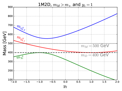
Figure 1: Mass spectra on the $1_{M}2_{D}$ system for $y_{1}=1$ as a function of $y_{2}$. The masses of the neutral states are depicted with continuous colored lines and by a black dashed line for the charged components. We use the subscripts $l$ and $h_{1,2}$ to refer respectively to light and heavy neutral eigenstates. These spectra illustrate the fact that the charged states combined with a singlet to form a Majorana triplet $3_{M}$ at the custodial points $y_{1}=\pm y_{2}$. The lightest neutral particle (LNP $\sim\chi_{l}^{0}$) is in this case generically a Majorana singlet, except near the custodial point $y_{2}=-y_{1}\equiv-1$ if $m_{M}>m_{\ast}\sim m_{D}$ where it forms a $3_{M}$. There is another $3_{M}$ at $y_{2}=y_{1}\equiv 1$ but its neutral component is not the LNP. See text for more details.

In each panel, the three solid lines correspond to the three neutral states, the lightest being a potential DM candidate. The horizontal dashed line corresponds to the charged states, with $m_{\chi^{\pm}}=m_{D}$. Focusing on the custodial point $y_{2}=-y_{1}$, we observe that clearly two of the neutral states, one of which has mass $m_{D}$ at $y_{2}=-y_{1}$, have an avoided level crossing. The latter corresponds to the combination of Weyl states that does not couple to the Higgs. This state is degenerate with the charged states, and altogether they form an $SU(2)$ triplet, $3_{M}$. Whether the LNP belongs to this triplet depends on the hierarchy between the bare Dirac and Majorana masses, $m_{M}\gtrsim m_{D}$ (left panel) or $m_{M}\lesssim m_{D}$ (right panel). More precisely, it is easy to verify that the levels cross when

$$m_{M}=m_{\ast}\equiv m_{D}-y_{1}^{2}\,{\eta^{2}v^{2}\over 2m_{D}}$$ (17)

were we assumed $y_{1}v\ll m_{D}$ with $y_{2}=-y_{1}$. If $m_{M}>m_{\ast}$, the LNP has mass $m_{D}$ and, together with the charged states, is in a triplet, $3_{M}$. If instead $m_{M}<m_{\ast}$, the LNP is a singlet, $1_{M}$. The latter state is a mixture of the original Majorana singlet $\chi_{0}$ and of the combination of Weyl states to which it couples through the Yukawa.

Away from the custodial point $y_{2}=-y_{1}$, we observe from Fig.1 that the mass eigenstates repel each other so that the mass of the LNP decreases while the mass of the charged partner stays constant, $m_{\chi^{\pm}}\equiv m_{D}$. Level repulsion thus explains why the LNP is also the lightest particle, and so potentially a dark matter candidate. For $m_{M}>m_{\ast}$ and working in the limit $|y_{1}+y_{2}|v\ll m_{M,D}$, it is easy to obtain that the mass splitting is given by

$$\Delta m=m_{\chi_{l}^{\pm}}-m_{\chi^{0}_{l}}\approx{a_{0}^{2}\over 4}(y_{1}+y_{2})^{2}{v^{2}\over m_{M}}\equiv(y_{1}+y_{2})^{2}{v^{2}\over 4\,m_{M}}$$

where the subscript $l$ stands for ”light”. So for $y_{1}+y_{2}\neq 0$, the LNP is a singlet, and this both for $m_{M}>m_{\ast}$ and $m_{M}<m_{\ast}$.

Finally, from Fig.1 we notice that the charged states combine with another singlet at $y_{1}=y_{2}$. This triplet is however heavier than the LNP. To recap, at the custodial points, the pattern of multiplet is as in (2.2.2), with $1_{M}2_{W}2_{W}\rightarrow 1_{M}1_{M}3_{M}$. Whether the LNP is in a $1_{M}$ or a $3_{M}$ is summarized in Table 2.

The $3_{M}4_{D}$ case

We discuss this next because it shares features with the $1_{M}2_{D}$ case. According to (2.2.2), we have the pattern $3_{M}4_{W}4_{W}\rightarrow 3_{M}3_{M}5_{M}$ at the custodial points. This is illustrated in Fig. 2 that shows that the neutral states follow always the same pattern as in the $1_{M}2_{D}$ system discussed above. The question is what is the mass spectrum of the charged partners? In the $3_{M}4_{D}$ case, it is the doubly charged state $\chi^{\pm\pm}$ that does not mix and so has mass $m_{D}$. At the custodial point $y_{1}=-y_{2}$ we observe from Fig.2 that it belongs to a $5_{M}$ formed with states (neutral and singly charged) that do not couple to the Higgs. This $5_{M}$ contains the LNP if $m_{M}>m_{\ast}$. If $m_{M}<m_{\ast}$, the LNP is instead in a $3_{M}$. The twist compared to the $1_{M}2_{D}$ case is that, away from $y_{1}=-y_{2}$, level repulsion brings down both the mass of the LNP and that of its singly charged partners, so that the LNP belongs to a nearly degenerate $3_{M}$ multiplet. The reason for this interesting behavior may be understood analytically by considering the hierarchies $y_{1,2}v\ll m_{D}\ll m_{M}$ or $y_{1,2}v\ll m_{M}\ll m_{D}$.

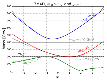
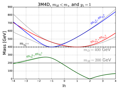
Figure 2: Mass spectra on the $3_{M}4_{D}$ system for $y_{1}=1$ as a function of $y_{2}$. The eigenmass of the neutral states are depicted with the same color coding as in Fig.1; singly charged eigenmass are shown as black dotted lines; the doubly charged states have constant mass $m_{D}$. These spectra are meant to illustrate the fact that the neutral and charged states combine in 2 Majorana $3_{M}$ and one $5_{M}$ of $SU(2)$ at the custodial points $y_{2}=\pm y_{1}\equiv\pm 1$ and, also, that they are nearly degenerate away from these points.

1. $m_{M}\gg m_{D}$ At $y_{1}=-y_{2}$, the LNP belongs to a $5_{M}$ of $SU(2)$ with mass $m_{D}$. The doubly charged components do not mix, so the mass is equal to $m_{D}$ for all $y_{1,2}$. Away from the custodial point $y_{1}=-y_{2}$, level repulsion brings down the mass of both the neutral and singly charged components. In the limit $y_{1,2}v\ll m_{D}\ll m_{M}$, we get near $y_{2}=-y_{1}$ that

   $$m_{\chi^{0}_{l}} \approx m_{D}-{a_{0}^{2}\over 4}(y_{1}+y_{2})^{2}{v^{2}\over m_{M}}$$ (18)

   $$\approx m_{D}-{1\over 6}(y_{1}+y_{2})^{2}{v^{2}\over m_{M}}$$

   while

   $$m_{\chi^{\pm}_{l}} \approx m_{D}-{a_{1}^{2}\tilde{a}_{1}^{2}\over 2(a_{1}^{2}+\tilde{a}_{1}^{2})}(y_{1}+y_{2})^{2}{v^{2}\over m_{M}}$$ (19)

   $$\approx m_{D}-{1\over 8}(y_{1}+y_{2})^{2}{v^{2}\over m_{M}}$$

   Thus, the mass splitting between the singly charged components and the LNP is

   $$\Delta m=m_{\chi^{\pm}_{l}}-m_{\chi^{0}_{l}}\approx{1\over 24}(y_{1}+y_{2})^{2}{v^{2}\over m_{M}}>0$$ (20)

   and the LNP is, at tree level, the lightest component of a nearly degenerate $3_{M}$ away from the custodial point. This is a generic conclusion: in all cases, the LNP is at tree level always the lightest component of the $SU(2)$ multiplet to which it belongs, and thus a priori a DM candidate. Why this is so is a bit mysterious but may be traced to the entries in the mass matrices, see (5-7). The outcome is that, somehow, level repulsion is stronger for the neutral particles than it is for their charged partners. We also infer that the custodial symmetry is keeping the $3_{M}$ nearly degenerate. We interpret this as being due to the fact that at the other custodial point, $y_{1}=y_{2}$, the lightest singly charged and neutral particles must again combine to form an exactly degenerate $SU(2)$ multiplet. As the mass of the doubly charged states stays constant, the only possibility is that the LNP is in a $3_{M}$, in agreement with what is observed Fig.2. Within the same approximations as above we get that, around $y_{1}=y_{2}$, the mass splitting between the charged component and the LNP is again

   $$\Delta m\approx{1\over 24}(y_{1}-y_{2})^{2}{v^{2}\over m_{M}}>0$$ (21)

   At the point $y_{1}=y_{2}$ the doubly charged states belong to a $5_{M}$, but this multiplet does not contain the LNP.

2. $m_{D}\gg m_{M}$ The main difference compared to $m_{D}\ll m_{M}$ is that the mass splittings are parametrically smaller. From inspection of the right panel of Fig.2, we see that the LNP is part of $3_{M}$ for all the range of Yukawa couplings; this multiplet is essentially the original Majorana triplet. Near $y_{2}=\pm y_{1}$, and for $m_{D}\gg m_{M}\gg y_{1,2}v$, we get

   $$\Delta m\approx{1\over 9}(y_{1}^{2}-y_{2}^{2})^{2}{v^{4}\over m_{D}^{3}}>0$$ (22)

   We see that the mass splitting is indeed parametrically smaller than in the case $m_{D}\ll m_{M}$ as it involves four powers of the Higgs vev, compare with Eq.(20). The mass splittings away from the custodial points depend too on the hierarchy of Majorana and Dirac masses, a feature already observed in Tait:2016qbg . This is illustrated diagrammatically in Fig.3 for $m_{M}\gg m_{D}$ (left panel) and $m_{M}\ll m_{D}$ (right panel). These Feynman graphs mean to illustrate the fact that mass splitting within custodial $SU(2)$ multiplets requires both $y_{1}\neq y_{2}$ and a Majorana mass insertion.

To recap, in the $3_{M}4_{D}$ system, at the custodial points, the pattern of multiplet is as in (2.2.2), with $3_{M}4_{W}4_{W}\rightarrow 3_{M}3_{M}5_{M}$. Whether the LNP is in a $5_{M}$ or a $3_{M}$ depends on the hierarchy between $m_{M}$ and $m_{D}$, as summarized in Table 2.

(a)

(b)

Figure 3: Contributions to mass splitting within n-plets for $m_{M}\gg m_{D}$ (3(a)) and $m_{D}\gg m_{M}$ (3(b)).

The $3_{M}2_{D}$ and $5_{M}4_{D}$ cases

have common features. The spectra of the neutral states are analogous to those of the $1_{M}2_{D}$ and $3_{M}4_{D}$ systems. The main difference is that all states (neutral, charged and, if they exist, doubly charged) mix, see Figs.4 and 5. Again, we distinguish $m_{M}>m_{\ast}\sim m_{D}$ and $m_{M}<m_{\ast}$.

1. $m_{M}\gg m_{D}$ At the custodial point $y_{2}=-y_{1}$, the LNP is the combination of Weyl states $\psi$ and $\tilde{\psi}$ that does not couple to the Higgs, and so has mass $m_{D}$. It is a $1_{M}$ in the $3_{M}2_{D}$ case (Fig.4), and is in a $3_{M}$ in the $5_{M}4_{D}$ one (Fig.5). Away from $y_{1}=-y_{2}$, level repulsion decreases the mass of the LNP. Interestingly, because all the states are mixed, we see in the left panel of Fig.4 (Fig.5) in the $3_{M}2_{D}$ (resp. $5_{M}4_{D}$) also the mass of the singly charged states $\chi_{l}^{\pm}$ (resp. doubly charged $\chi_{l}^{\pm\pm}$) decrease, so that at the other custodial point, $y_{1}=y_{2}$, the LNP belongs to a $3_{M}$ (resp. a $5_{M}$).

2. $m_{M}\ll m_{D}$ In this case, shown in the right panel of Fig.4 (Fig.5) the LNP is always in a $3_{M}$ (resp. $5_{M}$) in the $3_{M}2_{D}$ (resp. $5_{M}4_{D}$), as it is essentially the original Majorana $\chi_{0}$ with a small (in the limit $m_{M}\ll m_{D}$) admixture of $\psi_{1,2}^{0}$ states.

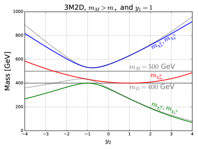
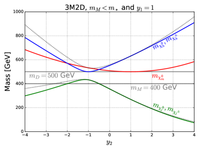
Figure 4: Mass spectra in the $3_{M}2_{D}$ system for $y_{1}=1$ as a function of $y_{2}$ for $m_{M}\gtrsim m_{\ast}$ (left panel) and $m_{M}\lesssim m_{\ast}$ (right panel). Masses of neutral states are depicted with continuous colored lines and the singly charged states with black dotted lines.

To recap, in the $3_{M}2_{D}$ ($5_{M}4_{D}$) system, and at the custodial points, the pattern of multiplet is as in (2.2.2), with $3_{M}2_{W}2_{W}\rightarrow 3_{M}3_{M}5_{M}$ (resp. $5_{M}4_{W}4_{W}\rightarrow 5_{M}5_{M}3_{M}$). Whether the LNP is in a $1_{M}$ or a $3_{M}$ (resp. a $3_{M}$ or a $5_{M}$) depends on the hierarchy between $m_{M}$ and $m_{D}$, see Table 2.

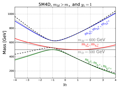
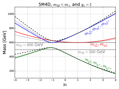
Figure 5: Mass spectra in the $5_{M}4_{D}$ system for $y_{1}=1$ as a function of $y_{2}$ for $m_{M}\gtrsim m_{\ast}$ (left panel) and $m_{M}\lesssim m_{\ast}$ (right panel). Masses of neutral states are depicted with continuous colored lines, for the singly charged states with black dotted lines and for the doubly charged states with black dashed lines.

2.2.3 Comments on effects of loop corrections

The conclusions of the previous section raises the question of the effects of radiative corrections. The custodial symmetry is broken at one-loop by electroweak corrections. For pure MDM, $\Delta m\propto\alpha_{2}m_{W}\sin^{2}\theta_{W}={\cal O}(100)$ MeV  Cirelli:2005uq . For mixed states, one expects that the situation is more complex. We have not studied the spectra at one-loop, so we will be sketchy, but we may refer to other works.

A first naive conclusion would be that, at the custodial points, as the LNP belongs to a multiplet of $SU(2)$, the situation must be the same as for MDM. That this is not quite the case is illustrated in Fig. 2 of ref. Tait:2016qbg for the $3_{M}4_{D}$ case when including NLO corrections. Beware that we used different conventions, so their case $y=y_{1}=y_{2}$ corresponds to our case $y=y_{1}=-y_{2}$. Regardless, their Fig. 2, illustrate the mass splittings dependence in $y$, at one-loop, at one of the custodial points. The LNP is noted $\chi_{1}^{0}\equiv\chi_{l}^{0}$ and at tree level it is in a $5_{M}$ if $m_{M}\gg m_{D}$ and a $3_{M}$ if $m_{M}\lesssim m_{D}$ (see our Fig. 2). One first sees in their Figure 2 that the mass splitting between the LNP and its singly charged partners depends on $y$. This is manifest for $m_{M}\gtrsim m_{D}$ (left panel), in which case the LNP has mass $m_{D}$ and is a Majorana built of the states $\psi$ and $\tilde{\psi}$. As these states have opposite hypercharge, their coupling to the neutral gauge bosons breaks the custodial symmetry even if at the custodial point $y_{1}=y_{2}$. For the case $m_{M}\lesssim m_{D}$ (right panel), the DM is essentially the original Majorana multiplet, with an admixture of Weyl states, so we expect this case to be closer to MDM. The dependence on $y$ must be mild, consistent with the right panel of Figure 2 of ref. Tait:2016qbg .

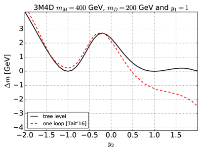
Figure 6: Mass splitting $\Delta m=m_{\chi_{l}^{\pm}}-m_{\chi_{l}^{0}}$ in the $3_{M}4_{D}$ system at tree level for $y_{1}=1$ as a function of $y_{2}$ for $m_{M}\gtrsim m_{\ast}$. The continuous black curve is the mass splitting at tree level. The red dashed curved is that at one-loop as obtained in ref. Tait:2016qbg .

Another naive conclusion would be that, away from the custodial points, the LNP remains the lightest component of the multiplet even at one-loop. After all, in the MDM, radiative corrections make the charged partners heavier than the neutral one. However, it seems that this is not the case either, see again ref. Tait:2016qbg . To be precise, if we remain in a regime in which the Yukawa couplings are not “too large”, one may expect that the dominant contributions to mass splitting are either determined from $|y_{1}|\neq|y_{2}|$ at tree level or at one-loop through gauge corrections; in both cases, the mass splittings are such that the LNP must be the lightest stable particle and thus potentially a dark matter candidate. If the Yukawa couplings get large however, this intuition may become invalid. For instance, one may get into a regime in which the mass of the LNP (and its charged partners) vanishes at tree level. This is possible if $y_{1}$ and $y_{2}$ are large and have the same sign (again, following our convention), see our Fig. 2. More precisely, one may check that this occurs if the product $m_{M}m_{D}\approx\eta^{2}y_{1}y_{2}v^{2}$, so that it may happen only for bare Majorana and Dirac masses below the TeV range provided $y_{1,2}\lesssim 4\pi$. For the sake of comparison, we show in Fig. 6 both the mass splitting at tree level derived here (black curve) and the result at one loop obtained in ref. Tait:2016qbg (we report here with red dashed line the red curve ref. Tait:2016qbg plotted the left panel of their Fig. 4). There we see that $\Delta m$ at one loop (red dashed) becomes negative when $y_{1}$ and $y_{2}$ are large and have the same sign, corresponding to the range of parameters for which the mass of the components of the lightest multiplet, and their mass splittings, are driven to zero at tree level (black continuous). That one-loop corrections can jeopardize the mass splitting in these conditions is thus perhaps not surprising. More strange is the fact, stated in ref. Tait:2016qbg , that $\Delta m$ becomes negative at one-loop even if the bare masses are large, which we suppose corresponds to $m_{M}m_{D}\gg\eta^{2}y_{1}y_{2}v^{2}$. Also, ref. Tait:2016qbg reports that this happens for $m_{M}\gtrsim m_{D}$. It could be interesting to explore further this feature.

3 HMDM: cosmology and astrophysics

The questions that we would like to address now is what is the mass range for which our candidates can accommodate all the DM (i.e. $\Omega_{DM}h^{2}=0.12$) and where, within this mass range, one would expect to get observable signals from the dark matter? As mentioned in the introduction, a complete treatment of these questions would require to take into account Sommerfeld corrections and bound state formation contribution to the annihilation cross-section for arbitrary Majorana-Dirac mixing. This is a difficult problem, which has only been tackled in details for specific SUSY-inspired scenarios, see e.g. Beneke:2016jpw ; Beneke:2016ync ; Beneke:2014gja . It is beyond the scope of this work to discuss these non-perturbative corrections in the generic HMDM. In what follows, we first analyze the viable parameter space in the perturbative limit. We then review how non-perturbative corrections affect these predictions for the limiting cases of pure MDM, and we provide an estimate of the Sommerfeld corrections for the pure quadruplet scenario. The latter is the only MDM case for which the Sommerfeld effect has not yet been explicitly studied in the literature. We close the discussion on non perturbative effects deriving the boundaries of the parameter space of the viable HMDM under study in this paper making use of the $SU(2)_{L}$ symmetric limit. Finally, we briefly comment on the possible prospects for DM direct and indirect searches. As we focus on candidates in the multi-TeV range, collider searches are not relevant and are altogether ignored in our discussions.

3.1 HMDM enlarging the MDM space: perturbative results

In this section we want to explore to which extent the parameter space of Minimal Dark Matter candidates is enlarged when different multiplets are coupled to the Higgs. This of course has been discussed case by case in many works, but as far as we know, no systematic comparison has yet been provided in the literature. For a given system, say the $3_{M}2_{D}$, the parameter space is a priori 4 dimensional, as we have two bare masses, $m_{M}$ and $m_{D}$ and two Yukawa couplings, $y_{1}$ and $y_{2}$. Fixing the relic abundance reduces this to 3 independent parameters (the “viable” DM candidates). For pure MDM, and thus zero Yukawa couplings, the mass of the viable DM candidate is fixed Cirelli:2005uq and for non-zero Yukawa couplings, the viable candidates should cover a domain in the plane $m_{M}-m_{D}$.

To estimate the boundary of the HMDM domains, we will make use of the electroweak symmetric limit. We will do so first because this tremendously simplifies the discussion, as we may neglect the mass splittings, mixing effects and annihilation through Higgs mediated processes in determining the abundance. A further motivation is that we may expect that the boundaries correspond to candidates for which Yukawa couplings are small, and so are close to the pure MDM cases. Last, the masses of MDM candidates are typically in the multi-TeV range, at least for MDM multiplet larger than the doublet, so that freeze-out occurs close or above the electroweak phase transition Cirelli:2005uq ; Cirelli:2009uv . Nevertheless, we should keep in mind that the symmetric approximation is better for the largest multiplets we consider.  We will comment further on the validity of this approximation towards the end of this section.

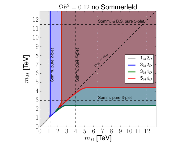
Figure 7: Viable parameter space in the perturbative $SU(2)_{L}$ symmetric approximation. Shaded regions enclose all models giving rise to $\Omega h^{2}=0.12$ for the 1M2D (in gray), for the 3M2D (in blue), for the 3M4D (in green) and 5M4D (in red). The limits of these contours, represented with thick continuous lines, have been obtained in the pure gauge limit, see text for details. The pure doublet, triplet, quadruplet and quintuplet limits including Sommerfeld corrections (and bounds state (B.S.) formation from Mitridate:2017izz in the 5-plet case) are indicated with dashed lines, see Sec. 3.2.

In the symmetric limit, we may neglect the mass splittings between the multiplet components, so that our ingredients are a mixture of pure Dirac and Majorana multiplets, which may co-annihilate with each other if their masses are within $\sim 10\%$ Griest:1990kh . On the other hand, in the presence of Yukawa interactions between the Dirac and the Majorana multiplets one expect that for $m_{M}\simeq m_{D}$ the coannihilation processes are quite efficient. To determine the boundary of the HMDM domains, we assume that the Yukawa couplings are sufficiently large for co-annihilations to be relevant, but that they are small enough so that the DM $n$-plet annihilation cross-section relevant for freeze-out is dominated by gauge interactions:

$$\sigma v_{{\rm eff},n}\simeq\frac{\zeta}{n^{2}}\frac{\alpha_{2}^{2}{\cal C}_{n}}{m_{DM}^{2}}$$ (23)

where $\zeta=1$ for the Majorana multiplet and 1/2 for the Dirac one, and ${\cal C}_{n}$ is a dimensionless coefficient that mainly depends on $n$ (see Sec. 3.2.3 below for more details). Also, we have neglected the mass of the gauge bosons. Following the treatment of Griest:1990kh , a proxy for the total annihilation cross-section at freeze-out for a mixture of Dirac and Majorana multiplets in interaction, would be:

$$\sigma v_{\rm eff} \simeq \frac{1}{g_{\rm eff}^{2}}\sum_{i=M,D}g_{i}^{2}\sigma v_{{\rm eff},i}\quad{\rm and}\quad g_{\rm eff}=\sum_{i=M,D}g_{i}$$ (24)

$$g_{i} = n_{i}(1+\Delta_{i})^{3/2}\exp(-\,x_{f}\Delta_{i})$$ (25)

where the sum runs over the two multiplets and $\Delta_{i}=(m_{i}-m_{0})/m_{0}$ with $m_{0}=\min(m_{M},m_{D})$, $n_{i}$ denotes the total number of degrees of freedom for the Majorana ($M$) or Dirac multiplet ($D$) and $\sigma v_{{\rm eff},i}$ corresponds to (23) for $n=n_{i}$. For concreteness, we will take $x_{f}=m_{0}/T_{f}=30$ when computing the cross-sections in the $SU(2)_{L}$ symmetric limit. We also use the standard approximate expression for the relic abundance

$$\Omega_{\rm DM}h^{2} \simeq \frac{1.07\,10^{9}\,x_{f}}{M_{pl}/{\rm GeV}\sqrt{g_{*}}\,\eta\,\sigma v_{eff}}\,,$$ (26)

valid for annihilation into an s-wave, with $M_{pl}=1.22\,10^{1}9$ GeV is the Planck mass and $g_{*}$ is the number of relativistic degrees of freedom at the time of freeze-out. Imposing $\Omega h^{2}=0.12$, we obtain the contours shown in Fig 7 with continuous colored lines. Notice that the material necessary to work out the expression of the relevant annihilation cross-sections is discussed in more detail in Sec. 3.2.

For each pair of Dirac and Majorana multiplets, the contours have asymptotic solutions corresponding to the pure (Majorana or Dirac) MDM candidates, linking each others approximatively along the diagonal $m_{M}=m_{D}$. Along this diagonal, the effective number of degrees of freedom is larger than for the pure cases, an effect which must be compensated by larger annihilation cross sections and thus smaller DM masses, compared to the pure cases. To put it simply, the situation is like having together two DM particles, with a similar mass, and so a larger abundance for fixed annihilation cross sections. This is the origin of the bottom-left pointing nose-shaped features observed in the contours along the $m_{M}\sim m_{D}$ direction. For larger Yukawa couplings DM depletion is more efficient due to the opening of more annihilation channels and more efficient co-annihilation channels, and so with extra terms contributing to eq. 25, see Griest:1990kh . Thus the contours feature a top-right pointing “nose” instead, i.e. the observed relic abundance would be obtained for a value $m_{M}=m_{D}$ larger than for the pure cases. Such features are observed in the plots of Ref. Tait:2016qbg for the case $3_{M}4_{D}$. Thus we infer that the shaded regions delimited by the contours (gray for 1M2D, blue for 3M2D, green for 3M4D and red for 5M4D) enclose all the candidates that would give rise to $\Omega h^{2}=0.12$ for a proper choice of the Yukawas $y_{1},y_{2}$. For a given model, larger couplings are required in the innermost regions when larger $(m_{D},m_{M})$ masses are considered. Outside the shaded regions, the DM candidates have an abundance below $\Omega h^{2}=0.12$.

To corroborate this simple, yet qualitative picture we have checked that the contour, obtained here in the electroweak symmetric limit, is in a good agreement with the numerical results for the dark matter abundance computed with micrOMEGAs, i.e. working in the $SU(2)_{L}$ broken limit, including mass splittings. For illustrative purposes, we show in Fig. 8 the results from a random scan over the parameter space of the $5_{M}4_{D}$ system, imposing $0.11<\Omega h^{2}<0.13$, $10^{-4}<|y_{1}|,|y_{2}|<4\pi$ and $1.5<m_{\chi},m_{\psi}<10\mbox{TeV}$. Let us emphasize that we do not incorporate the possible non perturbative effects in Fig. 8. The latter effects are discussed in the next section. Yet, we see that the viable parameter space of candidates obtained with micrOMEGAs (colored points) fit very well within the boundaries obtained in the $SU(2)_{L}$ symmetric limit, shown with dashed red contour (corresponding to the continuous red colored line in Fig. 7). The latter was obtained using the simple equations  (25) and (26).

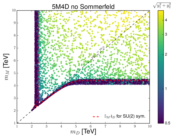
Figure 8: Viable parameter space in the perturbative 5M4D case for an explicit integration of the dark matter abundance with micrOMEGAs in the $SU(2)_{L}$-broken limit. All points give rise to $\Omega h^{2}\simeq 0.12$ for a value of the yukawa combination $\sqrt{y_{1}^{2}+y_{2}^{2}}$ indicated with the color code. Notice that we have considered $|y_{1}|,|y_{2}|$ as small as $10^{-4}$ but all points with $\sqrt{y_{1}^{2}+y_{2}^{2}}<0.5$ are shown in blue as they all end up in the contours of the 5M4D parameter space. With red dashed line, we show the (red) contour obtained in the $SU(2)_{L}$ symmetric limit for the 5M4D case in Fig. 7.

3.2 Dark matter abundance and Sommerfeld corrections

As mentioned above, computing Sommerfeld corrections in each HMDM case in general is a very involved calculation. In the $SU(2)_{L}$ symmetric limit, important simplifications of the Sommerfeld computation come from the fact that isospin is conserved in the annihilation and scattering processes. This allows to solve Schrodinger equations of 2-particle wavefunctions $\Psi_{I}$ of definite total isospin $I$, without mixing among them. As a consequence the Sommerfeld correction compution of a system of a large number $N$ of coupled differential equation is reduced to the resolution of $N^{\prime}<N$ uncoupled differential equations, which strongly simplifies the problem Strumia:2008cf ; deSimone:2014pda ; Garcia-Cely:2015khw ; Garcia-Cely:2015dda ; Garcia-Cely:2015quu ; Asadi:2016ybp ; Mitridate:2017izz . We will work in this framework in what follows.

3.2.1 Sommerfeld corrections in the $SU(2)_{L}$ symmetric limit

The $N^{\prime}$ above is associated to the number of possible irreducible representations ${\cal R}_{a}$ resulting from the direct product:

$$R_{i}\otimes R_{j}=\sum_{k=1}^{N^{\prime}}{\cal R}_{a}$$ (27)

where $R_{i}$ and $R_{j}$ denote the representation under $SU(2)_{L}$ of the two annihilating particles $i$ and $j$. Assuming zero mass gauge bosons in the unbroken $SU(2)_{L}$ limit, the potentials driving the $SU(2)_{L}$ long range interactions, take the form deSimone:2014pda :

$$V_{I_{a}}^{SU(2)}(r)=\frac{\alpha_{I_{a}}}{r}=\frac{\alpha_{2}}{r}\frac{1}{2}\left(C_{a}-C_{i}-C_{j}\right)\,,$$ (28)

where $\alpha_{2}=g/4\pi$, with the $SU(2)_{L}$ gauge coupling $g$, and the $C_{l}$ with $l=i,j$ and $a$ are the quadratic Casimir operators associated to the representation $R_{i}$,$R_{j}$ and ${\cal R}_{a}$. In the case of $SU(2)_{L}$, $C_{l}=I_{l}(I_{l}+1)$ where $I_{l}$ is the isospin corresponding to the representation $R_{l}$. Also, for annihilating particles with non zero hypercharge, we get a U$(1)_{Y}$ contribution to the potential that reads:

$$V^{U(1)}=\frac{\alpha^{\prime}}{r}=\frac{-\alpha_{2}t_{w}^{2}Y^{2}}{r}$$ (29)

where $\alpha^{\prime}=g^{\prime}/(4\pi)$, $g^{\prime}$ is the U(1)_Y gauge coupling related to $g$ by the tangent of the Weinberg angle $t_{w}$ and $Y=|Y_{i}|=|Y_{j}|$ is the absolute value the hypercharge of the particles $i$ and $j$.

In this way the total potential associated to a pair of particles annihilating in the total isospin state $I=I_{a}$ becomes

$$V_{I}=V_{I}^{SU(2)}+V^{U(1)}=\frac{\alpha_{I}+\alpha^{\prime}}{r}\leavevmode\nobreak\ .$$ (30)

In the zero mass approximation for the gauge bosons, each of the $N^{\prime}$ Shrödinger equations can be solved analytically. As a result, in the s-wave limit, the annihilation cross section $\sigma v_{I}$ of a given total isospin $I$ 2-particles state is given by:

$$\sigma v_{I}=S_{I}\,\sigma v_{I}^{\rm pert}\quad{\rm with}\quad S_{I}=\dfrac{-\pi a_{I}}{1-\exp(\pi/a_{I})}$$ (31)

where $S_{I}$ is the Sommerfeld factor that multiplies the perturbative annihilation cross section $\sigma v_{I}^{\rm pert}$ and $a_{I}=v/[2(\alpha_{I}+\alpha^{\prime})]$ where $v$ denote the relative velocity of the initial state particles. A priori, one should be concerned with the fact that at finite temperature, the gauge boson masses are non zero. The Higgs vev is temperature dependent and, in addition, the squared masses of the gauge bosons get an extra thermal mass contribution, see e.g. Cirelli:2007xd . We have however checked that due to these effects, for large representations, the Sommerfeld correction factors obtained resolving the Shrödinger equations including the thermal mass corrections agree with the Coulomb approximation of eq. (31) with an error $<1\%$ for $I\leq 2$ that is the maximum total isospin of a pair of standard model particles $XX^{\prime}$ into which $ij$ is annihilating into. See also Mitridate:2017izz for a careful treatment.

For computing the relic abundance in a pure case, we use eq. (26) with

$$\sigma v_{eff}=\zeta\sum_{ij}\dfrac{g_{i}g_{j}}{g_{eff}}\sigma v_{ij}$$ (32)

with $\zeta=1$ for self-conjugate particles and $1/2$ otherwise and $g_{eff}=\sum g_{i}$ with $g_{i}$ the number of degrees of freedom associated to the species $i$. Notice that the eq. (32) is only valid in the limit of negligible mass splittings between the (co-)annihilating particles that is relevant in the $SU(2)_{L}$ unbroken limit. The (co-)annihilation cross-sections of initial state particles $ij$ to any 2-body SM final state, $\sigma v_{ij}$, can easily be obtained from Feynmman rules. Making use of Clebsch-Gordan decomposition one can recast the $|ij\rangle$ contributions in terms of the isospin of 2 particle states $|I_{a}\rangle$, see appendix B for one example in the quadruplet case that is addressed in more detail below. As a result, for a dark matter candidate in a representation $R_{X}$ of $SU(2)_{L}$ with an isospin $I_{X}$ , in the simple case of $Y=0$, the effective cross section of eq. (32) reduces to:

$$\sigma v_{eff}=\frac{\zeta}{(2I_{X}+1)^{2}}\sum_{I}(2I+1)\,\sigma v_{I}\qquad[{\rm case}\,Y=0]\,,$$ (33)

where $I$ runs over the $I_{a}$ values with $a=1,..,N^{\prime}$. The cross-sections $\sigma v_{I}$ should be taken as in eq. (31). For $Y\neq 0$, extra contributions to $\sigma v_{eff}$ are expected from $U(1)_{Y}$ gauge bosons ($B_{\mu}$) insertions giving rise to annihilation cross sections proportional to ${\alpha^{\prime}}^{2}$, denoted by $\sigma v_{g^{\prime}}$, and cross sections proportional to $\alpha^{\prime}\alpha$, denoted by $\sigma v_{g^{\prime}g}$. The former results from $B_{\mu}$ mediated annihilations into two fermions or two Higgs, corresponding to $SU(2)_{L}$ singlet state, while the latter results from annihilations into both $B_{\mu}$ and an $SU(2)_{L}$ gauge boson, corresponding to $SU(2)_{L}$ triplet state. The overall Sommerfeld-corrected effective cross section relevant for the relic abundance computation thus reads:

$$\sigma v_{eff}=\frac{\zeta}{(2I_{X}+1)^{2}}\left(\sum_{I}(2I+1)S_{I}\sigma v_{I}^{\rm pert}+S_{I=1}\,\sigma v_{gg^{\prime}}^{\rm pert}+S_{I=0}\,\sigma v_{g^{\prime}}^{\rm pert}\right)\,\qquad[{\rm case}\,Y\neq 0]\,,$$ (34)

where, in the sum, $I$ runs over the $I_{a}$ values with $a=1,..,N^{\prime}$. Let us emphasize that the perturbative results, used for the plot in Fig. 7, can simply be obtained setting the Sommerfeld factors $S_{I}$ to 1.

3.2.2 One example: the pure quadruplet

We now illustrate in more detail how the method above can be applied to the pure 4-plet dark matter case. To our knowledge, this is the only pure case in which Sommerfeld corrections have not been previously computed explicitly. The 4-plet appears in a study of ref. Tait:2016qbg , a treatment at perturbative level only, while the treatment of the doublet, the triplet, the quintuplet and the 7-plet at non-perturbative level can readily be found in refs. Garcia-Cely:2015khw ; Garcia-Cely:2015quu ; Mitridate:2017izz ; Asadi:2016ybp ; Cirelli:2007xd ; Cirelli:2015bda ; Garcia-Cely:2015dda . Our results agree with the most recent updates, see Sec. 3.2.3 for more details.

We thus provide here a detailed computation of the Sommerfeld correction in the $SU(2)_{L}$ symmetric limit for the 4-plet. The Weyl multiplets that we are dealing with are:

$$\psi=\left(\begin{array}[]{c}\psi^{++}\\ \psi^{+}\\ \psi^{0}\\ \psi^{-}\end{array}\right)\qquad{\rm and}\qquad\tilde{\psi}=\left(\begin{array}[]{c}\tilde{\psi}^{+}\\ \psi^{0}\\ \psi^{-}\\ \psi^{--}\end{array}\right),$$ (35)

with opposite hypercharges equals to 1/2 and -1/2. In the scattering of 4 and $\bar{4}$, we know that $4\otimes\bar{4}=\sum_{a=1}^{N^{\prime}}{\cal R}_{a}=1\oplus 3\oplus 5\oplus 7$, where ${\cal R}_{a}$ are the $SU(2)_{L}$ representations of the 2-particle states with $a=1,..,4$ and isospins $I=\{0,1,2,3\}$. In the Coulomb limit, the associated $SU(2)_{L}$ potentials from eq. (28) take the values

$$V^{SU(2)}_{I}=\dfrac{-\alpha_{2}}{r}\left\{\frac{15}{4},\frac{11}{4},\frac{3}{4},\frac{-9}{4}\right\}\,,\qquad\mbox{ [4-plet]}$$ (36)

where we have used that the 4-plet has isospin $I_{4}=3/2$. In addition, the $U(1)_{Y}$ contribution reads

$$V^{U(1)}=-\alpha_{2}t_{w}^{2}Y^{2}_{4}/r\quad{\rm with}\quad Y_{4}=1/2\,.\qquad\mbox{ [4-plet]}$$ (37)

The overall potentials for $I=\{0,1,2,3\}$ involved in the long range physics computation associated to the annihilation of the 4 and $\bar{4}$ is thus a sum of $SU(2)_{L}$ potentials from eq. (36) and $V^{U(1)}$ as in eq. (30). Using (31) with $v\simeq 0.2$, we obtain the following Sommerfeld correction factors:

$$S_{I}=\{3.9,3.0,1.5,0.3\}\,.\qquad\mbox{ [4-plet]}$$ (38)

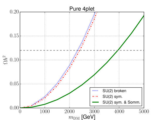
Figure 9: Pure 4-plet relic abundance $\Omega h^{2}$ including the Sommerfeld corrections (continuous brown) or not (red dotted) in the s-wave $SU(2)_{L}$ symmetric limit for the annihilation of quadruplet dark matter. With the blue dashed line we also show the results obtained with micrOMEGAs neglecting the Sommerfeld corrections in the $SU(2)_{L}$ broken case.

After extracting the $\sigma v_{I,g,g^{\prime}}$ following the method above, see appendix B for more details, the results for the relic abundances in the s-wave $SU(2)_{L}$ symmetric limit are summarized in Fig. 9 using:

$$\sigma v_{I=0}^{\rm pert}=\frac{75}{4}\frac{\alpha_{2}^{2}\pi}{M_{DM}^{2}},\quad\sigma v_{I=1}^{\rm pert}=\frac{125}{8}\frac{\alpha_{2}^{2}\pi}{M_{DM}^{2}},\quad\sigma v_{I=2}^{\rm pert}=6\frac{\alpha_{2}^{2}\pi}{M_{DM}^{2}}$$ (39)

$$\sigma v_{g^{\prime}g}^{\rm pert}=\frac{15}{2}\,t_{w}^{2}\,\frac{\alpha_{2}^{2}\pi}{M_{DM}^{2}},\quad\sigma v_{g^{\prime}}^{\rm pert}=\frac{43}{8}\,t_{w}^{4}\,\frac{\alpha_{2}^{2}\pi}{M_{DM}^{2}}\quad\mbox{ [4-plet]}$$ (40)

From Fig. 9, in order to account for $\Omega_{DM}h^{2}=0.12$, one would thus get $M_{DM}=2.4$ TeV in the perturbative limit, while taking into account the Sommerfeld corrections one gets $M_{DM}=3.9$ TeV. Also notice that, working in the $SU(2)_{L}$ broken limit using micrOMEGAs to compute the relic abundance, one obtains $M_{DM}=2.3$ TeV in the perturbative limit to account for $\Omega_{DM}h^{2}=0.12$ (see the blue dashed line in Fig. 9). This agrees with results of Tait:2016qbg in the $3_{M}4_{D}$ case in the limit of high mass triplet (i.e DM almost pure quadruplet). We are thus making a $\sim 4\%$ error working in the $SU(2)_{L}$ symmetric case in order to determine the relevant dark matter mass in the perturbative limit.

It has recently been pointed out that bound state formation (BSF) can provide an extra enhancement of the annihilation cross-section of minimal dark matter Asadi:2016ybp ; Mitridate:2017izz . In particular Asadi:2016ybp first showed that the rate of BSF in the triplet case is suppressed compared to direct annihilation. In Mitridate:2017izz , it was shown that BSF raises the mass of the 5-plet to 11.5 TeV, i.e. a $\sim$ 20% ($\sim$ 40%) correction to the mass (annihilation cross section) obtained with Sommerfeld corrections only while essentially no corrections appear in the 3-plet case.

It is beyond the scope of this paper to compute in detail the impact of BSF on freeze-out calculations. Here we just want to argue that the correction from BSF corresponding to the 4-plet case is expected to be smaller than for the 5-plet case. As noted by  Mitridate:2017izz , bound states can efficiently form even at temperatures $T\sim m_{\rm DM}/x_{f}$ larger than the corresponding bound state binding energies, because the dissociation rate can be suppressed with respect to naive expectations. Nonetheless, the intuition that smaller $E_{B}/T_{f}$ ratios (i.e. binding energy to freeze-out temperature) lead to smaller corrections from BSF remains valid, as shown in Mitridate:2017izz for the 3-plet case compared to the 5-plet case. Indeed for the former, $E_{B}\lesssim 0.05$ GeV at $T_{f}\sim 100$ GeV leads to a correction to the DM relic density at the % level, whereas for the latter, $E_{B}\lesssim 60$ GeV at $T_{f}\sim 460$ GeV leads to a 40% correction. In the case of the 4-plet, the most attractive potential (corresponding to the singlet two-particle state) has a strength of $15\alpha_{2}/4$, which corresponds to an $n=0$ bound state with binding energy $E_{B}\sim 4.2$ GeV at $T_{f}\sim 160$ GeV, following the method of estimation of  Mitridate:2017izz . As can be noted, $E_{B}/T_{f}$ is a factor $\sim 5$ smaller for the 4-plet than for the 5plet, thus the BSF correction to the relic abundance in the case of the 4-plet should be much less important.

3.2.3 HMDM: Sommerfeld correction of the viable parameter space

$n$	$I_{a}$	$\lambda_{a}$	$S_{I_{a}}$	$\sigma v_{I_{a}}^{\rm pert}$	$m_{DM}^{\rm pert}$ [TeV]	$m_{DM}^{\rm Som}$ [TeV]
2	$0$	$\frac{3}{4}+\frac{1}{4}t_{w}^{2}$	1.5	$\frac{3\pi\alpha_{2}^{2}}{8m_{DM}^{2}}$	1.1	1.1
	$1$	$-\frac{1}{4}+\frac{1}{4}t_{w}^{2}$	0.9	$\frac{25\pi\alpha_{2}^{2}}{16m_{DM}^{2}}$
3	$0$	$2$	2.3	$\frac{4\pi\alpha_{2}^{2}}{m_{DM}^{2}}$	2.4	3.
	$1$	$1$	1.6	$\frac{25\pi\alpha_{2}^{2}}{4m_{DM}^{2}}$
	$2$	$-1$	0.6	$\frac{\pi\alpha_{2}^{2}}{m_{DM}^{2}}$
4	$0$	$\frac{15}{4}+\frac{1}{4}t_{w}^{2}$	3.9	$\frac{75\pi\alpha_{2}^{2}}{4m_{DM}^{2}}$	2.4	3.9
	$1$	$\frac{11}{4}+\frac{1}{4}t_{w}^{2}$	3.	$\frac{125\pi\alpha_{2}^{2}}{8m_{DM}^{2}}$
	$2$	$\frac{3}{4}+\frac{1}{4}t_{w}^{2}$	1.5	$\frac{6\pi\alpha_{2}^{2}}{m_{DM}^{2}}$
	$3$	$-\frac{9}{4}+\frac{1}{4}t_{w}^{2}$	0.3	$-$
5	$0$	$6$	5.9	$\frac{60\pi\alpha_{2}^{2}}{m_{DM}^{2}}$	4.4	9.3
	$1$	$5$	5.	$\frac{125\pi\alpha_{2}^{2}}{4m_{DM}^{2}}$
	$2$	$3$	3.1	$\frac{21\pi\alpha_{2}^{2}}{m_{DM}^{2}}$
	$3$	$0$	1.	$-$

Table 3: For the pure multiplet of dimension $n$, the Isospins of the relevant 2-particle states are given by $I_{a}$, the potentials are driven by the $\lambda_{a}=-(\alpha_{I_{a}}+\alpha^{\prime})/\alpha_{2}$ couplings and, using $\sigma v_{I_{a}}^{\rm pert}$ together with the appropriate $\sigma v_{g,\,gg^{\prime}}^{\rm pert}$ in the 2-blet, 4-plet cases, one obtains $m_{DM}$ TeV for the dark matter mass including Sommerfeld corrections only in the $SU(2)_{L}$ symmetric limit ($m_{DM}^{\rm pert}$ is obtained without Sommerfeld corrections).

Figure 10: Boundaries of the viable parameter space of HMDM models in the $m_{M}-m_{D}$ plane represented with continuous lines when computing the relic abundance in the $SU(2)_{L}$ symmetric limit with Sommerfeld corrections for the 2-blet, 3-plet, 4-plet limiting cases. For the 5-plet, BSF corrections of Mitridate:2017izz are taken into account. As a guide for the eye, the perturbative results for the pure MDM cases are indicated with dashed lines.

The impact of Sommerfeld corrections on the viable space for dark matter is illustrated in Fig. 10. In order to derive the Sommerfeld enhanced pure n-plet limits we have followed the same recipe as in the case of the 4-plet above. For all the pure cases, corresponding to the limits $m_{M}\gtrsim(\lesssim)m_{D}$ of the models considered here, we summarize our findings in Tab. 3. These results were obtained considering an average velocity of $v\simeq 0.2$ in the computation of $S_{I_{a}}$ and the dark matter masses for the candidate giving rise to all the DM assuming $x_{f}=30$. For the doublet, as in the case of 4-plet (see eq. (40), one has to take into account $\sigma v_{g^{\prime}}$ and $\sigma v_{gg^{\prime}}$ (the $U(1)_{Y}$ and mixed $U(1)_{Y}$ & $SU(2)_{L}$ contribution as in eq. (34)). In the s-wave limit, for the doublet, we have found:

$$\sigma v_{g^{\prime}g}^{\rm pert}=\frac{3}{4}\,t_{w}^{2}\,\frac{\alpha_{2}^{2}\pi}{m_{DM}^{2}}\qquad\sigma v_{g^{\prime}}^{\rm pert}=\frac{43}{16}\,t_{w}^{4}\,\frac{\alpha_{2}^{2}\pi}{m_{DM}^{2}}\quad\mbox{ [doublet]}$$ (41)

Also notice that in Tab. 3, we only provide $\sigma v_{I_{a}}$ for $I_{a}<3$ as we focus on 2 body final states only which total isospin is always smaller than 3 in the SM. Our results are in agreement with the cases already available in the literature Garcia-Cely:2015quu ; Mitridate:2017izz .

The dark matter mass obtained to match $\Omega h^{2}=0.12$ when considering Sommerfeld corrections in the $SU(2)_{L}$ symmetric limit are provided in the last column of Tab. 3 and can be compared to the latest derived value present in the literature. Considering Sommerfeld corrections only, one can get from Beneke:2014hja $m_{DM}\simeq 1.2$ TeV in the doublet case, while in the 3-plet and in the 5-plet case ref. Mitridate:2017izz reports $m_{DM}\simeq$ 2.7 TeV and $m_{DM}\simeq$ 9.3 TeV respectively. We see that the $SU(2)_{L}$ symmetric limit provides a very good way to estimate Sommerfeld corrections at freeze-out. In the 5-plet case however, bound state formation changes the dark matter annihilation cross-section and eventually gives rise to the right abundance for $m_{DM}\simeq$ 11.5 TeV Mitridate:2017izz . We have not tried to re-evaluate this effect here but we account for it in our summary plot of Fig. 10. In the latter plot, we make use of our results from Tab. 3 except in the case of the 5-plet where we use the BSF result from Mitridate:2017izz . The interpolating regions between the pure cases have been obtained with the same method as in the perturbative case, see Sec. 3.1, Eq.25.

3.3 Dark matter detection prospects

As regards prospects for DM detection, we hereby discuss the main features and effects that can be expected when moving from the pure MDM scenarios to the HMDM ones, without providing a full-fledged analysis that would also require computing the conditions for the right relic abundances of the various HMDM scenarios.

3.3.1 Direct detection

HMDM has spin-dependent and spin-independent interactions at tree level with quarks. As mentioned in the introduction, we have checked numerically that spin-dependent cross-section (computed at tree-level) always appear to be way beyond the reach of current experiments, we will thus focus here on spin independent (SI) scattering. For the latter, the relevant processes for HMDM are scatterings with quarks via Higgs exchange at tree level and, at loop level, scattering with quarks and gluons via exchange of electroweak bosons. In the limit of pure MDM candidate, the tree level interactions vanish and the leading interaction occurs via loops Cirelli:2005uq ; Hisano:2015rsa . Here we mainly discuss the salient features of the spin independent scattering cross-section on nucleons at tree level, with particular emphasis on the 5M4D model, while arguing about the expected behavior at loop level. A detailed computation of the scattering cross-section in HMDM should be the subject of a dedicated analysis that is beyond the scope of this work.

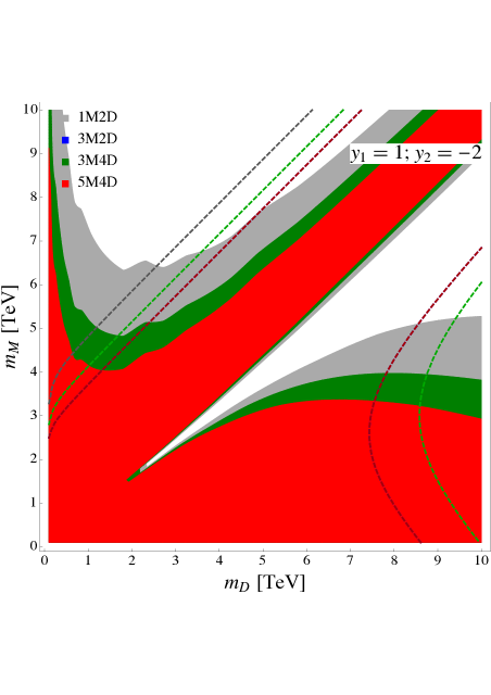
Figure 11: Tree-level DM-nucleon SI scattering in the plane $m_{D}-m_{M}$ for all the models considered in this work. Colored regions are excluded by prospects of limits from the XENON1T experiment Aprile:2015uzo for $y_{1}=1$ and $y_{2}=-2$. Colored lines show contours of DM composition, the lower right ones denote $|Z_{11}^{M}|^{2}=0.999$ while the upper left ones correspond to $|Z_{11}^{M}|^{2}=0.001$. The contours of the $3_{\textrm{\footnotesize M}}2_{\textrm{\footnotesize D}}$ model overlap with those of the $5_{\textrm{\footnotesize M}}4_{\textrm{\footnotesize D}}$ model.

From the discussion in sec. 2.2.1 focusing on the custodial symmetry limit, it appears that the DM coupling to the Higgs (driving the direct detection cross-section at tree-level) is expected to be maximal in the limit $m_{M}\rightarrow m_{D}$ and $y_{1}\rightarrow y_{2}$ while it is expected to vanish for $m_{M}\rightarrow m_{D}$ and $y_{1}\rightarrow-y_{2}$. Let us see how this goes beyond the custodial limit. The SI scattering cross section for the DM candidate off a nucleon $N$ at tree level for the model $M$ is Cheung:2013dua :

$$\sigma^{M}_{\rm SI}\propto\dfrac{\mu^{2}}{m_{h}^{4}}(c^{M}_{h\chi^{0}_{l}\chi^{0}_{l}})^{2}\leavevmode\nobreak\ ,$$ (42)

where $\mu={m_{\chi^{0}_{l}}m_{N}}/{(m_{\chi^{0}_{l}}+m_{N})}$ is the nucleon-DM reduced mass, $m_{h}$ is the Higgs mass, and the coefficient $c^{M}_{h\chi^{0}_{l}\chi^{0}_{l}}$ contains the Higgs-DM coupling in the model $M$, and is:

$$c^{M}_{h\chi^{0}_{l}\chi^{0}_{l}}=-\dfrac{c_{M}}{\sqrt{2}}\left[y_{1}(Z^{M}_{11})^{*}(Z^{M}_{12})^{*}+y_{2}(Z^{M}_{11})^{*}(Z^{M}_{13})^{*}\right]\leavevmode\nobreak\ .$$ (43)

The matrix ${\bf Z}^{M}$ defines the rotation to the mass basis with the $\{\chi^{0}_{\alpha}\}$ states ordered from light to heavy states ($\alpha=l,m,h$). Going from the basis used in Sec. 2.2.1, with $\{\chi^{0}_{i}\}$ indices $i=1,2,3$ not pointing to any mass ordering, to the basis used here just simply imply a permutation of the entries of the transformation matrix of Eq. (11) in order to get ${\bf Z}^{M}$. Finally, the coefficients $c_{M}$ for all the models are:

$$c_{\rm 1M2D}=1,\leavevmode\nobreak\ \leavevmode\nobreak\ \leavevmode\nobreak\ c_{\rm 3M2D}=\dfrac{1}{\sqrt{2}},\leavevmode\nobreak\ \leavevmode\nobreak\ \leavevmode\nobreak\ c_{\rm 3M4D}=\sqrt{\dfrac{2}{3}},\leavevmode\nobreak\ \leavevmode\nobreak\ \leavevmode\nobreak\ c_{\rm 5M4D}=\dfrac{1}{\sqrt{2}}\leavevmode\nobreak\ .$$ (44)

We show in Fig. 11 the present and future exclusion region from XENON1T experiment Aprile:2015uzo ; Aprile:2017iyp from the calculation at tree-level for a choice of Yukawa couplings $y_{1}=1$ and $y_{2}=-2$. As can be seen, there are common features to all models considered above. First, there are parts of the parameter space where the cross section is suppressed, even for light DM that is largely mixed. In Fig. 11, this translates as incursions of the white area into the colored regions illustrating the reach of Xenon 1T for a given choice of $y_{1}$ and $y_{2}$. Around these “blind spots”, the coupling of the Higgs to DM that mediates the tree-level interactions is suppressed, as has been discussed in the literature for the case of the supersymmetric neutralino Cheung:2012qy and the $1_{M}2_{D}$ model Cheung:2013dua ; Calibbi:2015nha . Second, for a given size of the Yukawa couplings and for large enough masses the composition of DM seems to depend on $m_{M}-m_{D}$. Indeed, as observed in Hill:2013hoa , in this limit the dynamics can be described in terms of two parameters only, $\Delta=(m_{M}-m_{D})/2$ and $a=|y_{1}+y_{2}|/2$ for real Yukawa couplings. The reason is that the DM-Higgs effective vertex is in this case proportional to $a^{2}/\sqrt{a^{2}+(\Delta/2m_{W})^{2}}$. In the $\Delta\to 0$ limit (i.e. along the diagonal), the cross section is thus maximised. This behavior generalizes the dependence in $\Delta$ and $a$ that we observed in the custodial symmetry limit in Sec.2.2.1 .

Let us now illustrate the above discussion in a concrete HMDM model. We focus on the 5M4D model for which we have already discussed the viable parameter space in Sec. 3.1. In particular the results of Fig. 8 were obtained from a random scan in the $SU(2)_{L}$ broken limit with all calculations at tree-level using micrOMEGAs. Here we project in Fig. 12 the same parameter space in the $m_{M}-m_{D}$ plane with, this time, the gradient color corresponding to the values of the spin independent scattering cross-section computed with micrOMEGAs, $\sigma_{SI}$, on the left hand (LH) side and $|y_{1}+y_{2}|$ on the right hand (RH) side. Let us first focus on the LH side plot illustrating the $\sigma_{SI}$ dependence on the parameters. The largest values of $\sigma_{SI}$ clearly appear to cluster along the diagonal, i.e. $\Delta=0$ as expected from the above discussion. On the other hand, the dark blue colored points correspond to the vanishing tree-level $\sigma_{SI}$. Most of them appear to cluster at the boundary of the viable parameter space, i.e. for vanishing Yukawas or pure MDM cases. In addition, we see that some more blue points appear to have a suppressed $\sigma_{SI}$ outside from the boundaries, within the mixed region. Comparing the LH side plot to the RH side plot, illustrating the dependence in $|y_{1}+y_{2}|$, it appears that there is clearly a close correlation between suppressed $\sigma_{SI}$ (darker points on the RH side) and vanishing $|y_{1}+y_{2}|$. In the mixed region, we know from Fig. 8 that such points typically have non-zero $\sqrt{y_{1}^{2}+y_{2}^{2}}$ values. As a consequence, we can see that, in the 5M4D case (at tree-level), points with suppressed $\sigma_{SI}$ and non negligible Yukawa couplings can be obtained $y_{1}\rightarrow-y_{2}$ corresponding to $a\rightarrow 0$ in agreement with the above discussion.

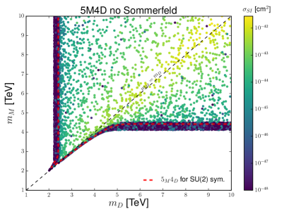
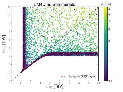
Figure 12: Viable parameter space in the perturbative 5M4D case for an explicit integration of the dark matter abundance with micrOMEGAs in the $SU(2)_{L}$-broken limit as in Fig. 8. All points give rise to $\Omega h^{2}\simeq 0.12$ and the value of the corresponding $\sigma_{SI}$ and $|y_{1}+y_{2}|$ are indicated with the color code in the left and right plot respectively. With red dashed line, we show the contour obtained in the $SU(2)_{L}$ symmetric limit for the 5M4D case in Fig. 7.

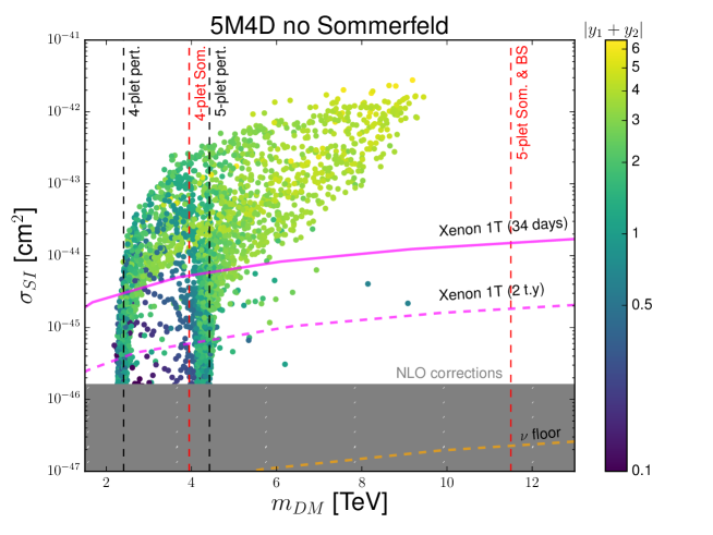
Figure 13: $\sigma_{SI}$ in the 5M4D case for an explicit integration of the dark matter abundance with micrOMEGAs in the $SU(2)_{L}$-broken limit as in Fig. 8. All points give rise to $\Omega h^{2}\simeq 0.12$. The gray zone is expected to be strongly affected by NLO corrections as in this zone $\sigma_{SI}<1.6\,10^{-46}$ cm${}^{2}=\sigma_{SI,{\rm 4-plet}}^{\rm NLO}$ computations. The vertical black dashed lines indicate the DM mass obtained in the $SU(2)_{L}$ symmetric limit for the pure 4-plet and 5-plet case without sommerfeld corrections. The red dashed lines include the Sommerfeld correction for the 4-plet and the Sommerfeld + Bound state effects from Mitridate:2017izz in the 5-plet case. The continuous magenta line denote the current constraints from the Xenon 1T experiment Aprile:2017iyp and the magenta line shows the reach prospects for the same experiment Aprile:2015uzo . The dashed orange line shows the “discovery limit” from Billard:2013qya .

Figure 13 shows the same information as the LH plot of Fig. 12 but now in the $\sigma_{SI}$ vs. $m_{DM}$ plane, where the color represents the value of $|y_{1}+y_{2}|\propto a$. Again, all the points in the scatter plot reproduce the observed relic abundance computed without taking into account Sommerfeld nor bound-state formation. However, we may expect that these corrections will only shift (and enlarge) the overall shape of the points cloud to the right, and that the features will remain the same. Around the pure limits, ie near the vertical dashed lines without (with) non-perturbative corrections in black (red) color, the tree-level $\sigma_{SI}$ can typically be much smaller than for the mixed regions (away from the vertical dashed lines) and even below the direct detection experiments prospects. In these regions, we expect that the loop corrections are quite relevant. As a guide for the eye, we show with gray color in Fig. 13, the region where electroweak corrections already appear to be relevant. In practice we do not expect to have cross-sections, including NLO corrections, to sum up well below the pure 4-plet result $\sigma_{SI,{\rm 4-plet}}^{\rm NLO}=1.6\,10^{-46}$ cm² obtained in Hisano:2015rsa . In practice, Higgs mediated loop corrections should provide some extra features. Some estimation of this effect is already provided by Hill:2014yka ; Hill:2013hoa for the $1_{M}2_{D}$ and the $3_{M}2_{D}$ models taking into account two-loop contribution to the twist-2 gluon effective operator and running of the Wilson coefficients down to the nuclear scale. The main feature that we underline here also is that the tree level cross-section dominates in the region of $m_{M}=m_{D}$ or equivalently $\Delta=0$. Beyond tree-level, loop-level blind spots could occur because of a cancellation between the contribution from the scalar and the twist-2 operators, as shown e.g. in Hill:2014yka ; Hill:2013hoa .

3.3.2 Discussion of indirect searches

In section 3.2, we estimated the impact of the Sommerfeld effect on the relic abundance, which is clearly important in estimating the mass of the thermal candidates. By the same token, the Sommerfeld corrections can affect DM annihilation in the recent Universe, like at the Galactic Centre, where the DM is highly non-relativistic. In particular, they can lead to annihilation cross sections that are much larger (potentially by orders of magnitude) than the canonical value $\sim 3\cdot 10^{-26}$ cm²/s required for the relic abundance Hisano:2004ds . This is particularly true for large multiplet Minimal Dark Matter candidates, not only because they tend to be in the TeV mass regime, substantially larger than the mass of the $Z$ and $W$ gauge bosons, but also because their multiplet contain particles multiply charged under $U(1)_{\rm em}$. This aspect of MDM has been much studied, starting with Cirelli:2007xd (see also Cirelli:2009uv ). Calculating the Sommerfeld corrections is infamously involved because of resonant behaviors due to mass splittings, and the results have been somewhat varying in time (but eventually converged, see Figure 7 Cirelli:2015bda and Figure 3 in Garcia-Cely:2015dda ).

A pure fermionic minimal dark matter candidate is strongly constrained by searches for gamma-ray spectral features (e.g. monochromatic lines) from the GC region by the HESS collaboration Ackermann:2013yva . The 3-plet and the 5-plet are both are excluded if the DM profile is cuspy, NFW or Einasto, while the 5-plet is marginally viable if the profile is cored, isothermal or Burkert Cohen:2013ama ; Hryczuk:2014hpa ; Cirelli:2015bda ; Garcia-Cely:2015dda ; Ovanesyan:2016vkk ; Lefranc:2016fgn .  Does mixing of a Majorana multiplet with two Weyl states bring anything new? To fully address this question one should calculate the non-perturbative corrections for each possible viable candidate, taking into account mixing and also the existence of new channels associated to Higgs exchange, etc. This is a very technical task, way beyond our scope. Instead we merely argue that, if anything, mixing brings some new freedom, possibly relaxing the constraints from gamma-rays observations. The key point is basic, and has been partly considered in some works for the case of Minimal Dark Matter candidates, either to enhance or deplete the annihilation cross sections at low velocities, see e.g. Chun:2012yt ; Chun:2016cnm . It rest on the fact that Sommerfeld corrections that lead to mono-chromatic gamma-rays are very sensitive to the mass splitting between the DM candidate and its charged partners. For pure MDM candidates, the splitting is set by electroweak corrections, while mixed states receive an extra contribution from their direct coupling to the Higgs. Simple criteria to assess the impact of mass splitting on the Sommerfeld corrections are given in Slatyer:2009vg . Suppressing the effect of excited states requires that the mass splitting $\Delta$ is larger than the kinetic energy of the DM, $m_{\rm DM}v^{2}/2\leq\sim\Delta m$. Less obvious, but natural, it that the binding energy of DM in an attractive channel, $\sim\alpha^{2}m_{\rm DM}$ must be smaller than the energy required to produced an excited state, $\Delta m$. Regardless, changing $\Delta m$ allows to move around the position of the resonant peaks, as is for instance illustrated in Chun:2012yt and can potentially help in evading the gamma-ray constraints.

4 Conclusion

In the Minimal Dark Matter framework, a dark matter candidate is the neutral component of an electroweak multiplet of dimension $n$. As such a candidate has only gauge interactions, all observables are in principle univocally determined. In particular, its relic abundance through thermal freeze-out can match the cosmological observed value only for a unique dark matter mass. Also, their signal in both direct and indirect searches are fixed, at least modulo astrophysical uncertainties. As such, they are very useful benchmark WIMP candidates. Focusing on fermionic cases, the highest possible representation, at least if ones want to avoid Landau poles at low energies, is a Majorana 5-plet. A nice feature of such candidate is that it may be automatically long-lived, without the need of imposing some symmetry, as its coupling to SM degrees of freedom can only come through a dimension 6 operator. Lower dimension representations are nevertheless of much interest, if anything because they correspond to specific corners of well-motivated candidates. For instance, a Majorana triplet is equivalent to a pure wino candidate, while a doublet is a pure higgsino. The latter has non-zero hypercharge, and so is excluded by direct detection if it is a pure Dirac state but mixing with a triplet or a singlet (i.e. a bino), through the Higgs doublet, makes it Majorana (or quasi-Dirac).

In this work we have extended on the Minimal Dark Matter framework by considering all pairs of electroweak fermionic multiplets (up to a 5-plet) that can have a Yukawa coupling with the Standard Model Higgs doublet, a framework we dubbed Higgs coupled Minimal Dark Matter or HMDM. As in the MDM framework, avoiding the Landau pole for the EW coupling at a low scales, we end up considering four possible models of mixed Majorana and Dirac fermions, including the $1_{M}2_{D},3_{M}2_{D},3_{M}4_{D}$ and $5_{M}4_{D}$. Because of mixing, and the coupling to the Higgs, the phenomenology of such scenarios is much more involved than in the pure MDM case. Several cases have been already considered in the literature, in particular in relation with the neutralino candidates to which we alluded to above. The $3_{M}4_{D}$ case has only been discussed recently, see Tait:2016qbg . To our knowledge, the $5_{M}4_{D}$ case the has not yet been considered in the literature.

Our purpose was to provide a unified presentation of the different cases. Doing so, we have first provided a detailed analysis of the dark matter mass spectrum. We have made use of the existence of a custodial symmetry that arises for specific Yukawa couplings and that provides a way to understand many features of the mass spectra, including the emergence of quasi-degenerate electroweak multiplets and an understanding of the mass splitting between the components. In particular, we have shown that, at tree level, the lightest neutral particle (LNP) is always the lightest component, and so potentially a dark matter candidate. This conclusion has however to be moderated as one-loop corrections may change the hierarchy of masses, a fact that we have inferred from Tait:2016qbg and their analysis of the $3_{M}4_{D}$ case. Next, we have then analyzed the viable parameter space of HMDM both in the perturbative approximation and taking into account non-perturbative effects. Indeed, as is the case of MDM, the candidates considered here are expected to be particularly affected by Sommerfeld effect and also, in the case of largest $SU(2)_{L}$ representations, by bound state formation. The calculations of these phenomena is notoriously delicate, and even more so for mixed candidates, and have only been tackled for specific mixed scenarios associated to SUSY phenomenology. Here, we have merely extracted the boundaries of the viable HMDM parameter space, and this using the electroweak symmetric limit, both for the perturbative regime and for non-perturbative corrections. This procedure greatly simplifies the calculations and yet, we argued, provides a good proxy to more precise calculations. Doing so, we have provided the first estimate of the mass of a (quasi-pure) 4-plet candidate, taking into the Sommerfeld effects. Figure 10 and Tab. 3 summarize our findings for all the considered HMDM scenarios.

The HMDM framework greatly increases the range of possible DM candidates. Their coupling to the Higgs, on top of gauge bosons, also greatly enhances the possibility for their search through direct detection experiments. This is clear using the parameter space of HMDM candidates using only perturbative calculations. We have argue that the same should hold taking into account the correction on the mass of the dark matter candidates due to Sommerfeld effect. In particular, several candidate in the multi-TeV range should be within reach of the current Xenon-1T experiment and, a fortiori, of future direct detection experiments. We have not addressed in details indirect detection, for which Sommerfeld corrections are particularly at the same time very relevant and very sensitive to the precise characteristics of not only the LNP particle, but also of the other components of the electroweak multiplet to which it may belong, and in particular the mass splittings, which in the HMDM scenario arises at tree level, except at exceptional custodial points. A complete analysis would require to take into account a full one-loop calculation of the mass spectrum, as well as the Sommerfeld effects. Such study remains to be done for the $3_{M}4_{D}$ and $5_{M}4_{D}$ cases, which are of particular interest as they point to DM candidate in the multi-TeV mass range. We leave this however for future works.

Appendix A Generators of $SU(2)$ and other useful formulas

We enlist all the generators of the su(2) algebra up to the 6-dimensional representation

$$T_{2}^{1}=\left(\begin{array}[]{cc}0&{1\over 2}\\ {1\over 2}&0\end{array}\right)\,,\quad T_{2}^{2}=\left(\begin{array}[]{cc}0&-{i\over 2}\\ {i\over 2}&0\end{array}\right)\,,\quad T_{2}^{3}=\left(\begin{array}[]{cc}{1\over 2}&0\\ 0&-{1\over 2}\end{array}\right)\,,$$ (51)

$$T_{3}^{1}=\left(\begin{array}[]{ccc}0&{1\over\sqrt{2}}&0\\ {1\over\sqrt{2}}&0&{1\over\sqrt{2}}\\ 0&{1\over\sqrt{2}}&0\end{array}\right)\,,\quad T_{3}^{2}=\left(\begin{array}[]{ccc}0&{-i\over\sqrt{2}}&0\\ {i\over\sqrt{2}}&0&{-i\over\sqrt{2}}\\ 0&{i\over\sqrt{2}}&0\end{array}\right)\,,\quad T_{3}^{3}=\left(\begin{array}[]{ccc}1&0&0\\ 0&0&0\\ 0&0&-1\end{array}\right)\,,$$ (61)

$$T^{1}_{4}\!=\!\left(\!\!\begin{array}[]{cccc}0&{\sqrt{3}\over 2}&0&0\\ {\sqrt{3}\over 2}&0&1&0\\ 0&1&0&{\sqrt{3}\over 2}\\ 0&0&{\sqrt{3}\over 2}&0\end{array}\!\!\right)\,,\ T^{2}_{4}\!=\!\left(\!\!\begin{array}[]{cccc}0&\textrm{-}i{\sqrt{3}\over 2}&0&0\\ i{\sqrt{3}\over 2}&0&\textrm{-}i&0\\ 0&i&0&\textrm{-}i{\sqrt{3}\over 2}\\ 0&0&i{\sqrt{3}\over 2}&0\end{array}\!\!\right)\,,\ T^{3}_{4}\!=\!\left(\!\!\begin{array}[]{cccc}{3\over 2}&0&0&0\\ 0&{1\over 2}&0&0\\ 0&0&\textrm{-}{1\over 2}&0\\ 0&0&0&\textrm{-}{3\over 2}\end{array}\!\!\right)\,,$$ (74)

$$T^{1}_{5}\!=\!\left(\!\!\begin{array}[]{ccccc}0&1&0&0&0\\ 1&0&{\sqrt{6}\over 2}&0&0\\ 0&{\sqrt{6}\over 2}&0&{\sqrt{6}\over 2}&0\\ 0&0&{\sqrt{6}\over 2}&0&1\\ 0&0&0&1&0\end{array}\!\!\right)\,,\ T^{2}_{5}\!=\!\left(\!\!\begin{array}[]{ccccc}0&\textrm{-}i&0&0&0\\ i&0&\textrm{-}i{\sqrt{6}\over 2}&0&0\\ 0&i{\sqrt{6}\over 2}&0&\textrm{-}i{\sqrt{6}\over 2}&0\\ 0&0&i{\sqrt{6}\over 2}&0&\textrm{-}i\\ 0&0&0&i&0\end{array}\!\!\right)\,,\ T^{3}_{5}\!=\!\left(\!\!\begin{array}[]{ccccc}2&0&0&0&0\\ 0&1&0&0&0\\ 0&0&0&0&0\\ 0&0&0&\textrm{-}1&0\\ 0&0&0&0&\textrm{-}2\end{array}\!\!\right)\,,$$ (90)

$$T_{6}^{1}\!=\!\left(\!\!\begin{array}[]{cccccc}0&{\sqrt{5}\over 2}&0&0&0&0\\ {\sqrt{5}\over 2}&0&\sqrt{2}&0&0&0\\ 0&\sqrt{2}&0&{3\over 2}&0&0\\ 0&0&{3\over 2}&0&\sqrt{2}&0\\ 0&0&0&\sqrt{2}&0&{\sqrt{5}\over 2}\\ 0&0&0&0&{\sqrt{5}\over 2}&0\end{array}\!\!\right)\,,\ T_{6}^{2}\!=\!\left(\!\!\begin{array}[]{cccccc}0&-i{\sqrt{5}\over 2}&0&0&0&0\\ i{\sqrt{5}\over 2}&0&-i\sqrt{2}&0&0&0\\ 0&i\sqrt{2}&0&-i{3\over 2}&0&0\\ 0&0&i{3\over 2}&0&-i\sqrt{2}&0\\ 0&0&0&i\sqrt{2}&0&-i{\sqrt{5}\over 2}\\ 0&0&0&0&i{\sqrt{5}\over 2}&0\end{array}\!\!\right),$$ (103)

$$T_{6}^{3}=\left(\begin{array}[]{cccccc}{5\over 2}&0&0&0&0&0\\ 0&{3\over 2}&0&0&0&0\\ 0&0&{1\over 2}&0&0&0\\ 0&0&0&-{1\over 2}&0&0\\ 0&0&0&0&-{3\over 2}&0\\ 0&0&0&0&0&-{5\over 2}\end{array}\right)\,.$$ (110)

We use the tensor formalism where

$$\left(\!\begin{array}[]{c}\chi_{1111}\\ \sqrt{4}\chi_{1112}\\ \sqrt{6}\chi_{1122}\\ \sqrt{4}\chi_{1222}\\ \chi_{2222}\end{array}\!\right)\equiv\left(\!\begin{array}[]{c}\chi^{++}\\ \chi^{+}\\ \chi^{0}\\ \chi^{-}\\ \chi^{--}\end{array}\!\right) \left(\!\begin{array}[]{c}\psi_{111}\\ \sqrt{3}\psi_{112}\\ \sqrt{3}\psi_{122}\\ \psi_{222}\end{array}\!\right)\equiv\left(\!\begin{array}[]{c}\psi^{++}\\ \psi^{+}\\ \psi^{0}\\ \psi^{-}\end{array}\!\right)$$ (129)

$$\left(\!\begin{array}[]{c}\tilde{\psi}_{111}\\ \sqrt{3}\tilde{\psi}_{112}\\ \sqrt{3}\tilde{\psi}_{122}\\ \tilde{\psi}_{222}\end{array}\!\right)\equiv\left(\!\begin{array}[]{c}\tilde{\psi}^{+}\\ \tilde{\psi}^{0}\\ \tilde{\psi}^{-}\\ \tilde{\psi}^{--}\end{array}\!\!\!\right) \left(\!\begin{array}[]{c}\chi_{11}\\ \sqrt{2}\chi_{12}\\ \chi_{22}\end{array}\!\right)\equiv\left(\!\begin{array}[]{c}\chi^{+}\\ \chi^{0}\\ \chi^{-}\end{array}\!\right)$$ (145)

These normalization factors appearing above just simply correspond to $\sqrt{{\rm Binomial}[n-1,i-1]}$, where $n$ is the length of the multiplet and $i$ is the position of the component of charge $Q$ in the $T_{3}$ basis. For the $a_{Q}$ coefficients defined in (7), we have thus for e.g. the neutral component of the Majorana triplet $a_{\chi^{0}}=\sqrt{{\rm Binomial}[2,1]}=\sqrt{2}$ while for the neutral component of the Majorana quintuplet we have $a_{\chi^{0}}=\sqrt{{\rm Binomial}[4,2]}=\sqrt{6}$.

Appendix B Cross-sections for two-particle states in $SU(2)$ symmetric limit

On can recast the cross-sections $\sigma v_{ij}$, where $ij$ characterizes the two initial state particles, in terms of the $\sigma v_{I}$ associated to eigenstates of total isospin $I$ in the $SU(2)_{L}$ symmetric limit. For the latter purpose, one has to derive the coefficients $C_{I_{a},ij}$ relating a total isospin 2 particle states $|I_{a}\rangle$ to a sum states $|ij\rangle$. This is obtained inverting the Clebsch-Gordan decomposition of $|ij\rangle$ in terms of $|I_{a}\rangle$. The relation between cross-sections then reads:

$$\sigma v_{ij}^{\rm pert}=\sum_{I}|C_{I,ij}|^{2}\sigma v_{I}^{\rm pert}$$ (146)

where $I$ runs over the $I_{a}$ values with $a=1,..,N^{\prime}$. In our case, we have obtained the analystica expressions of $\sigma v_{ij}$ making use of Calchep.

Below, we detail the derivation of the different contributions to the total annihilation cross-section in the case of the quadruplet. Notice that we have provided the relevant $\sigma v_{I}^{\rm pert}$ for all cases of interest for this paper in Tab. 3. In the quadruplet case, one considers the annihilation of a $4$ with a $\bar{4}$ with hypercharges $Y_{4}=1/2$ and $Y_{\bar{4}}=-1/2$ and respectively. The index $i$ in $\sigma v_{ij}$ denotes the charge of annihilating component of the 4 while the index $j$ denotes the charge of annihilating component of the $\bar{4}$. The $SU(2)_{L}$ only contributions to the annihilation cross are given by:

• $Q_{tot}=i+j=0$

  $$\sigma v_{0,0} = \sigma v_{I=0}/4+\sigma v_{I=1}/20+\sigma v_{I=2}/4=\sigma v_{+,-}$$ (147)

  $$\sigma v_{++,--} = \sigma v_{I=0}/4+9\sigma v_{I=1}/20+\sigma v_{I=2}/4=\sigma v_{-,+}$$ (148)

• $Q_{tot}=i+j=1$

  $$\sigma v_{++,-} = 3\sigma v_{I=1}/10+\sigma v_{I=2}/2=\sigma v_{0,+}$$ (149)

  $$\sigma v_{+,0} = 2/5\sigma v_{I=1}$$ (150)

• $Q_{tot}=i+j=2$

  $$\sigma v_{++,-} = \sigma v_{I=2}/2=\sigma v_{+,+}\,.$$ (151)

Notice that in this case $\sigma v_{ij}\neq\sigma v_{ji}$ as the charge indices are not the good representative quantum numbers to specify the isospin projection of each of the annihilating particles that have opposite hypercharges.

Using eq. (26), with $\zeta=1/2$ for a Dirac dark matter particle, the relic abundance can be computed using

$$\sigma v_{eff}=\sum_{ij}\dfrac{g_{i}g_{j}}{g^{2}_{tot}}\sigma v_{ij}=\dfrac{1}{16} ( \sigma v_{0,0}+\sigma v_{+,-}+\sigma v_{-,+}+\sigma v_{++,--}+2(\sigma v_{+,0}+\sigma v_{0,+})+2\sigma v_{++,-}$$ (152)

$$+ 2\sigma v_{+,+}+2\sigma v_{++,0}+2\sigma v_{++,+})$$

where the index $i$ and $j$ of the annihilation cross-section $\sigma v_{ij}$ refer here to the charges of $\psi$ and $\tilde{\psi}$ respectively. Using the Clebsh-Gordan decomposition one can extract the $\sigma v_{I}$, with $I=0,1,2,3$, from the $SU(2)_{L}$ contributions to $\sigma v_{ij}$, i.e. the non zero contributions for $g^{\prime}\rightarrow 0$. The expression of $\sigma v_{eff}$ can then be rewritten as:

$$\sigma v_{eff}=\dfrac{1}{16}\left(\sigma v_{I=0}+3\sigma v_{I=1}+5\sigma v_{I=5}+\sigma v_{g^{\prime}}+\sigma v_{g^{\prime}g}\right)$$ (153)

with $\sigma v_{g^{\prime}}$ and $\sigma v_{gg^{\prime}}$ being the $U(1)_{Y}$ and mixed $U(1)_{Y}$ & $SU(2)_{L}$ contribution as in eq. (34). In the s-wave limit, we have thus found for the 4-plet the results of eq. (40).

References

- (1) Marco Cirelli, Nicolao Fornengo, and Alessandro Strumia. Minimal dark matter. Nucl.Phys., B753:178–194, 2006, hep-ph/0512090.
- (2) Marco Cirelli and Alessandro Strumia. Minimal Dark Matter: Model and results. New J. Phys., 11:105005, 2009, 0903.3381.
- (3) Luca Di Luzio, Ramona Gr ber, Jernej F. Kamenik, and Marco Nardecchia. Accidental matter at the LHC. JHEP, 07:074, 2015, 1504.00359.
- (4) Lawrence M. Krauss and Frank Wilczek. Discrete Gauge Symmetry in Continuum Theories. Phys. Rev. Lett., 62:1221, 1989.
- (5) Mario Kadastik, Kristjan Kannike, and Martti Raidal. Matter parity as the origin of scalar Dark Matter. Phys. Rev., D81:015002, 2010, 0903.2475.
- (6) Natsumi Nagata, Keith A. Olive, and Jiaming Zheng. Weakly-Interacting Massive Particles in Non-supersymmetric SO(10) Grand Unified Models. JHEP, 10:193, 2015, 1509.00809.
- (7) Andrea De Simone, Veronica Sanz, and Hiromitsu Phil Sato. Pseudo-Dirac Dark Matter Leaves a Trace. Phys. Rev. Lett., 105:121802, 2010, 1004.1567.
- (8) Junji Hisano, Koji Ishiwata, and Natsumi Nagata. QCD Effects on Direct Detection of Wino Dark Matter. JHEP, 06:097, 2015, 1504.00915.
- (9) E. Aprile et al. Physics reach of the XENON1T dark matter experiment. JCAP, 1604(04):027, 2016, 1512.07501.
- (10) Richard J. Hill and Mikhail P. Solon. Standard Model anatomy of WIMP dark matter direct detection II: QCD analysis and hadronic matrix elements. Phys. Rev., D91:043505, 2015, 1409.8290.
- (11) Valentin Lefranc, Emmanuel Moulin, Paolo Panci, Filippo Sala, and Joseph Silk. Dark Matter in lines: Galactic Center vs dwarf galaxies. JCAP, 1609(09):043, 2016, 1608.00786.
- (12) Grigory Ovanesyan, Tracy R. Slatyer, and Iain W. Stewart. Heavy Dark Matter Annihilation from Effective Field Theory. Phys. Rev. Lett., 114(21):211302, 2015, 1409.8294.
- (13) Matthew Baumgart, Ira Z. Rothstein, and Varun Vaidya. Constraints on Galactic Wino Densities from Gamma Ray Lines. JHEP, 04:106, 2015, 1412.8698.
- (14) Marco Cirelli, Thomas Hambye, Paolo Panci, Filippo Sala, and Marco Taoso. Gamma ray tests of Minimal Dark Matter. JCAP, 1510(10):026, 2015, 1507.05519.
- (15) Camilo Garcia-Cely, Alejandro Ibarra, Anna S. Lamperstorfer, and Michel H. G. Tytgat. Gamma-rays from Heavy Minimal Dark Matter. JCAP, 1510(10):058, 2015, 1507.05536.
- (16) John David March-Russell and Stephen Mathew West. WIMPonium and Boost Factors for Indirect Dark Matter Detection. Phys. Lett., B676:133–139, 2009, 0812.0559.
- (17) John Ellis, Feng Luo, and Keith A. Olive. Gluino Coannihilation Revisited. JHEP, 09:127, 2015, 1503.07142.
- (18) Benedict von Harling and Kalliopi Petraki. Bound-state formation for thermal relic dark matter and unitarity. JCAP, 1412:033, 2014, 1407.7874.
- (19) Mark B. Wise and Yue Zhang. Stable Bound States of Asymmetric Dark Matter. Phys. Rev., D90(5):055030, 2014, 1407.4121. [Erratum: Phys. Rev.D91,no.3,039907(2015)].
- (20) Seng Pei Liew and Feng Luo. Effects of QCD bound states on dark matter relic abundance. JHEP, 02:091, 2017, 1611.08133.
- (21) Pouya Asadi, Matthew Baumgart, Patrick J. Fitzpatrick, Emmett Krupczak, and Tracy R. Slatyer. Capture and Decay of Electroweak WIMPonium. JCAP, 1702(02):005, 2017, 1610.07617.
- (22) Andrea Mitridate, Michele Redi, Juri Smirnov, and Alessandro Strumia. Cosmological Implications of Dark Matter Bound States. JCAP, 1705(05):006, 2017, 1702.01141.
- (23) Grigory Ovanesyan, Nicholas L. Rodd, Tracy R. Slatyer, and Iain W. Stewart. One-loop correction to heavy dark matter annihilation. Phys. Rev., D95(5):055001, 2017, 1612.04814.
- (24) L. Rinchiuso. Search for dark matter signals with 10-year obsevations by H.E.S.S. towards the Galactic Centre. talk: Moriond 2017, 2017.
- (25) T. Hambye, F. S. Ling, L. Lopez Honorez, and J. Rocher. Scalar Multiplet Dark Matter. JHEP, 07:090, 2009, 0903.4010.
- (26) Ayres Freitas, Susanne Westhoff, and Jure Zupan. Integrating in the Higgs Portal to Fermion Dark Matter. JHEP, 09:015, 2015, 1506.04149.
- (27) Rakhi Mahbubani and Leonardo Senatore. The Minimal model for dark matter and unification. Phys. Rev., D73:043510, 2006, hep-ph/0510064.
- (28) Francesco D’Eramo. Dark matter and Higgs boson physics. Phys. Rev., D76:083522, 2007, 0705.4493.
- (29) R. Enberg, P. J. Fox, L. J. Hall, A. Y. Papaioannou, and M. Papucci. LHC and dark matter signals of improved naturalness. JHEP, 11:014, 2007, 0706.0918.
- (30) Timothy Cohen, John Kearney, Aaron Pierce, and David Tucker-Smith. Singlet-Doublet Dark Matter. Phys.Rev., D85:075003, 2012, 1109.2604.
- (31) Clifford Cheung and David Sanford. Simplified Models of Mixed Dark Matter. JCAP, 1402:011, 2014, 1311.5896.
- (32) Lorenzo Calibbi, Alberto Mariotti, and Pantelis Tziveloglou. Singlet-Doublet Model: Dark matter searches and LHC constraints. JHEP, 10:116, 2015, 1505.03867.
- (33) Shankha Banerjee, Shigeki Matsumoto, Kyohei Mukaida, and Yue-Lin Sming Tsai. WIMP Dark Matter in a Well-Tempered Regime: A case study on Singlet-Doublets Fermionic WIMP. JHEP, 11:070, 2016, 1603.07387.
- (34) Carlos E. Yaguna. Singlet-Doublet Dirac Dark Matter. Phys. Rev., D92(11):115002, 2015, 1510.06151.
- (35) Martin Beneke, Aoife Bharucha, Andrzej Hryczuk, Stefan Recksiegel, and Pedro Ruiz-Femenia. The last refuge of mixed wino-Higgsino dark matter. JHEP, 01:002, 2017, 1611.00804.
- (36) Athanasios Dedes and Dimitrios Karamitros. Doublet-Triplet Fermionic Dark Matter. Phys.Rev., D89(11):115002, 2014, 1403.7744.
- (37) Tim M. P. Tait and Zhao-Huan Yu. Triplet-Quadruplet Dark Matter. JHEP, 03:204, 2016, 1601.01354.
- (38) David Tucker-Smith and Neal Weiner. Inelastic dark matter. Phys. Rev., D64:043502, 2001, hep-ph/0101138.
- (39) James McKay, Pat Scott, and Peter Athron. Pitfalls of iterative pole mass calculation in electroweak multiplets. 2017, 1710.01511.
- (40) M. Beneke, A. Bharucha, F. Dighera, C. Hellmann, A. Hryczuk, S. Recksiegel, and P. Ruiz-Femenia. Relic density of wino-like dark matter in the MSSM. JHEP, 03:119, 2016, 1601.04718.
- (41) M. Beneke, C. Hellmann, and P. Ruiz-Femenia. Non-relativistic pair annihilation of nearly mass degenerate neutralinos and charginos III. Computation of the Sommerfeld enhancements. JHEP, 05:115, 2015, 1411.6924.
- (42) Bryan Ostdiek. Constraining the minimal dark matter fiveplet with LHC searches. Phys. Rev., D92:055008, 2015, 1506.03445.
- (43) Camilo Garcia-Cely and Julian Heeck. Phenomenology of left-right symmetric dark matter. 2015, 1512.03332. [JCAP1603,021(2016)].
- (44) Chiara Arina, Mikael Chala, Victor Martin-Lozano, and Germano Nardini. Confronting SUSY models with LHC data via electroweakino production. JHEP, 12:149, 2016, 1610.03822.
- (45) Marco Cirelli, Filippo Sala, and Marco Taoso. Wino-like Minimal Dark Matter and future colliders. JHEP, 10:033, 2014, 1407.7058. [Erratum: JHEP01,041(2015)].
- (46) Qian-Fei Xiang, Xiao-Jun Bi, Peng-Fei Yin, and Zhao-Huan Yu. Exploring Fermionic Dark Matter via Higgs Precision Measurements at the Circular Electron Positron Collider. 2017, 1707.03094.
- (47) Ahmed Ismail, Eder Izaguirre, and Brian Shuve. Illuminating New Electroweak States at Hadron Colliders. Phys. Rev., D94(1):015001, 2016, 1605.00658.
- (48) Eugenio Del Nobile, Marco Nardecchia, and Paolo Panci. Millicharge or Decay: A Critical Take on Minimal Dark Matter. JCAP, 1604(04):048, 2016, 1512.05353.
- (49) Kim Griest and David Seckel. Three exceptions in the calculation of relic abundances. Phys. Rev., D43:3191–3203, 1991.
- (50) Alessandro Strumia. Sommerfeld corrections to type-II and III leptogenesis. Nucl. Phys., B809:308–317, 2009, 0806.1630.
- (51) Andrea De Simone, Gian Francesco Giudice, and Alessandro Strumia. Benchmarks for Dark Matter Searches at the LHC. JHEP, 06:081, 2014, 1402.6287.
- (52) Camilo Garcia-Cely, Michael Gustafsson, and Alejandro Ibarra. Probing the Inert Doublet Dark Matter Model with Cherenkov Telescopes. JCAP, 1602(02):043, 2016, 1512.02801.
- (53) Marco Cirelli, Alessandro Strumia, and Matteo Tamburini. Cosmology and Astrophysics of Minimal Dark Matter. Nucl. Phys., B787:152–175, 2007, 0706.4071.
- (54) M. Beneke, Charlotte Hellmann, and P. Ruiz-Femenia. Heavy neutralino relic abundance with Sommerfeld enhancements - a study of pMSSM scenarios. JHEP, 03:162, 2015, 1411.6930.
- (55) E. Aprile et al. First Dark Matter Search Results from the XENON1T Experiment. Phys. Rev. Lett., 119(18):181301, 2017, 1705.06655.
- (56) Clifford Cheung, Lawrence J. Hall, David Pinner, and Joshua T. Ruderman. Prospects and Blind Spots for Neutralino Dark Matter. JHEP, 05:100, 2013, 1211.4873.
- (57) Richard J. Hill and Mikhail P. Solon. WIMP-nucleon scattering with heavy WIMP effective theory. Phys. Rev. Lett., 112:211602, 2014, 1309.4092.
- (58) J. Billard, L. Strigari, and E. Figueroa-Feliciano. Implication of neutrino backgrounds on the reach of next generation dark matter direct detection experiments. Phys. Rev., D89(2):023524, 2014, 1307.5458.
- (59) Richard J. Hill and Mikhail P. Solon. Standard Model anatomy of WIMP dark matter direct detection I: weak-scale matching. Phys. Rev., D91:043504, 2015, 1401.3339.
- (60) Junji Hisano, Shigeki. Matsumoto, Mihoko M. Nojiri, and Osamu Saito. Non-perturbative effect on dark matter annihilation and gamma ray signature from galactic center. Phys.Rev., D71:063528, 2005, hep-ph/0412403.
- (61) Timothy Cohen, Mariangela Lisanti, Aaron Pierce, and Tracy R. Slatyer. Wino Dark Matter Under Siege. JCAP, 1310:061, 2013, 1307.4082.
- (62) M. Ackermann et al. Dark matter constraints from observations of 25 Milky Way satellite galaxies with the Fermi Large Area Telescope. Phys.Rev., D89:042001, 2014, 1310.0828.
- (63) Andrzej Hryczuk, Ilias Cholis, Roberto Iengo, Maryam Tavakoli, and Piero Ullio. Indirect Detection Analysis: Wino Dark Matter Case Study. JCAP, 1407:031, 2014, 1401.6212.
- (64) Eung Jin Chun, Jong-Chul Park, and Stefano Scopel. Non-perturbative Effect and PAMELA Limit on Electro-Weak Dark Matter. JCAP, 1212:022, 2012, 1210.6104.
- (65) Eung Jin Chun, Sunghoon Jung, and Jong-Chul Park. Very Degenerate Higgsino Dark Matter. JHEP, 01:009, 2017, 1607.04288.
- (66) Tracy R. Slatyer. The Sommerfeld enhancement for dark matter with an excited state. JCAP, 1002:028, 2010, 0910.5713.