Finite temperature effects in helical quantum turbulence

Abstract

We perform a study on the evolution of helical quantum turbulence at different temperatures by solving numerically the Gross-Pitaevskii and the Stochastic Ginzburg-Landau equations, using up to $4096^{3}$ grid points with a pseudospectral method. We show that for temperatures close to the critical the fluid described by these equations can act as a classical viscous flow, with the decay of the incompressible kinetic energy and the helicity becoming exponential. The transition from this behavior to the one observed at zero temperature is smooth as a function of temperature. Moreover, the presence of strong thermal effects can inhibit the development of a proper turbulent cascade. We provide anzats for the effective viscosity and friction as a function of the temperature.

I Introduction

In experiments of superfluids and Bose-Einstein condensates (BECs) a highly disorganized and chaotic behavior, known as quantum turbulence, can be observed Vinen and Niemela (2002); Henn et al. (2009); Barenghi et al. (2014). At zero temperature quantum flows are characterized by their lack of viscosity, and by having all of their vorticity concentrated along vortex filaments with quantized circulation Feynman (1955); Donnelly (1991). But at finite temperatures dissipative effects creep in. Landau and Tisza’s two fluid model Landau and Lifshitz (2004), where a mixture of superfluid and normal fluid coexist and interact (with the ratio between the two determined by the temperature), is perhaps the most simple way to represent the finite temperature dynamics of superfluids and BECs.

Based on the two fluid model, the Hall-Vinen-Bekarevich-Khalatnikov (HVBK) model Hall and Vinen (1956); Bekarevich and Khalatnikov (1961) adds a term accounting for the “mutual friction” between the normal and superfluid components. This model has been successful in, for example, explaining the Taylor-Couette instability in liquid helium Barenghi and Jones (1987). It has also been used to study turbulent flows; for example, Roche et al. (2009) found that there is a strong locking between both fluid components and that both develop a turbulent cascade, Shukla et al. (2015) found the existence of both an inverse and a forward cascade in the two dimensional case, and shell models based on the HVBK model were developed and used to study the mutual friction terms Wacks and Barenghi (2011); Boué et al. (2015), intermittency Boué et al. (2013), and scaling exponents Shukla and Pandit (2016). An alternative to the HVBK model is the vortex filament model Schwarz (1985), which, as the name implies, takes the vortex filaments into account explicitly by modeling them as classical Eulerian vortices of negligible width which evolve under the Biot-Savart law. As mutual friction can also be added to this model, it has been used to study quantum turbulence at finite temperatures Khomenko et al. (2015, 2016). But two important aspects of quantum turbulence are omitted in these two models. One is the lack of compressibility effects, and thus, of sound waves. The other is vortex reconnection. While in the HVBK model the former is omitted completely, as the fluid is averaged over volumes larger than the vortex width, in the vortex filament model it is introduced phenomenologically.

There is another family of models to study finite temperature effects based on extensions of the Gross-Pitaevskii equation (GPE). At zero or near zero temperatures the GPE, for which quantized vortices are exact solutions which can reconnect with no extra ad-hoc assumptions, is a very succesful model for BECs Proukakis and Jackson (2008). Moreover, a hydrodynamic analogy can be easily obtained from the GPE by means of the Madelung transformation, and it has been shown that at the larger scales its turbulent solutions match those of classical turbulence Nore et al. (1997a); Clark di Leoni et al. (2017). There are various ways of generalizing the GPE for studying finite-temperature effects Berloff et al. (2014). These include solving the spectrally truncated version of the equations Davis et al. (2001); Connaughton et al. (2005), coupling them with a Boltzmann equation describing the evolution of the thermalized modes as in the Zaremba-Nikuni-Griffin model Zaremba et al. (1999), or simply adding a phenomenological dissipation term Pitaevskii (1959); Choi et al. (1998). Previous studies of these models have concentrated on understanding the thermalization processes Davis et al. (2001); Krstulovic and Brachet (2011a, b); Shukla et al. (2013), on investigating single vortex decay Kobayashi and Tsubota (2006); Jackson et al. (2009); Rooney et al. (2010); Allen et al. (2014); Rooney et al. (2016), or on modelling traps with several vortices Rooney et al. (2013); Stagg et al. (2015) in configurations similar to experiments of BECs Neely et al. (2013); Moon et al. (2015); Kim et al. (2016); Seo et al. (2017). However, few studies have focused on the properties of the turbulent motions and on how finite temperature effects come into play in this regime.

In this context, it is worth noting that the study of quantum turbulence has garnered much interest in the past years. Two of the main areas of work have been establishing the differences between classical and quantum turbulence Barenghi et al. (2014); Paoletti et al. (2008), and understanding the dynamics of Kelvin waves Fonda et al. (2014); Clark di Leoni et al. (2015). The usual picture of quantum turbulence (see, for example, Vinen and Niemela (2002)) goes by the following: while at the larger scales the nonlinear energy transfer in quantum flows is mediated by the interaction between vortices and reconnection processes Meichle et al. (2012), and the turbulent flow resembles that of a classical fluid, at scales smaller than the mean intervortex length Kelvin waves are believed to be the ones responsible for the energy transfer, thus generating Kelvin wave turbulence Kozik and Svistunov (2004); L’vov and Nazarenko (2010); Boué et al. (2011, 2015); Clark di Leoni et al. (2015). Nonlinear interaction of Kelvin waves leads to the creation of phonons Vinen et al. (2003), which are finally responsible for the depletion of incompressible kinetic energy in quantum turbulence Nore et al. (1997b); Clark di Leoni et al. (2017). Additionally, recently it was shown that at zero temperature helical quantum turbulence (i.e., for flows with non-zero large-scale helicity) develops a dual cascade of energy and of helicity reminiscent of the dual cascade observed in classical helical flows, and that the emission of phonons also result in the depletion of helicity Clark di Leoni et al. (2017). The presence of such a dual cascade, where both energy and helicity are being transferred from the larger to the smaller scales to be finally dissipated, has a strong impact in the evolution and decay of turbulence. In classical flows, this dual cascade has received significant attention (see, e.g., Brissaud et al. (1973); Chen et al. ; Teitelbaum and Mininni ; Moffatt (2014)), as well as the effects of helicity in the evolution and statistical properties of turbulence. As a result, understanding how helical flows and their dual cascade are affected by the interaction with the effective thermal dissipation in finite temperature models will be the first main objective of the present work.

Indeed, the overall purpose of this paper is to study finite temperature effects on a helical quantum flow in high resolution numerical simulations of the truncated Gross-Pitaesvkii equation, with the thermal states being generated by the Stochastic Ginzburg Landau method Berloff et al. (2014). Our results show that for high temperatures the quantum fluid described by this model can behave as a classical viscous flow, with the decay of energy and of helicity becoming exponential in time, and with the development of the dual turbulent cascade being hindered. The transition from the zero to the high temperature behavior is smooth as a function of the temperature, as long as the temperature is smaller than the critical. As a second objective, we will profit from the high spatial resolution of our simulations to provide anzats for the effective viscosity as a function of the temperature. The structure of the paper is as follows. In Sec. II we outline the physical model used, and describe the simulations we performed. The main results are presented in Sec. III. Finally, closing comments are presented in Sec. IV.

II The finite temperature model

In this section we first present a brief summary of some key concepts and definitions of the zero temperature model (the GPE), used in this work as the starting point for the finite temperature model. Then, we explain how to generate finite temperature states using the Stochastic Ginzburg Landau equation (SGLE), following the method outlined in Krstulovic and Brachet (2011a, b), and how to use these states in quantum turbulence simulations solving the GPE. Finally, we give details of a large number of high resolution simulations performed for the present study.

II.1 The Gross-Pitaevskii equation

At zero (or near zero) temperatures, a field of weakly interacting bosons can be appropriately described by the GPE,

$$i\hbar\frac{\partial\Psi}{\partial t}=-\frac{\hbar^{2}}{2m}\nabla^{2}\Psi+g|\Psi|^{2}\Psi,$$ (1)

where $\Psi$ is the wavefunction of the condensate, $m$ is the mass of the bosons, and $g$ is proportional to the bosons scattering length. The GPE conserves the total energy

$$E=\int_{V}dV\left(\frac{\hbar^{2}}{2m}|\nabla\Psi|^{2}+\frac{g}{2}|\Psi|^{4}\right),$$ (2)

the momentum

$${\bf P}=\int_{V}dV\frac{i\hbar}{2}\left(\Psi\nabla\bar{\Psi}-\bar{\Psi}\nabla\Psi\right),$$ (3)

(where the overbar denotes complex conjugate), and the total number of particles

$$\mathcal{N}=\int_{V}dV|\Psi|^{2}.$$ (4)

A hydrodynamical description of the flow can be recovered via the Madelung transformation

$$\Psi({\bf r},t)=\sqrt{\frac{\rho({\bf r},t)}{m}}e^{im\phi({\bf r},t)/\hbar},$$ (5)

where $\rho({\bf r},t)$ is the fluid mass density, and $\phi({\bf r},t)$ is the velocity potential. Applying this transformation to the GPE yields the equations for an ideal barotropic fluid plus an extra term with the gradient of the so-called quantum pressure. This hydrodynamical description is useful to separate the total energy into different components Nore et al. (1997b). These are respectively the kinetic energy

$$E_{k}=\int_{V}dV\frac{1}{2}\rho|{\bf v}|^{2},$$ (6)

(which in turn can be separated into an incompressible component $E^{i}_{k}$ and a compressible one $E^{c}_{k}$ using a Helmholtz decomposition of the velocity field), the quantum energy

$$E_{q}=\int_{V}dV\frac{\hbar^{2}}{2m^{2}}(\nabla\sqrt{\rho})^{2},$$ (7)

and the internal (or potential) energy

$$E_{p}=\int_{V}dV\frac{g}{2m^{2}}\rho^{2}.$$ (8)

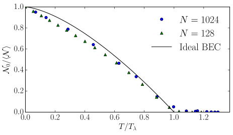
Figure 1: (Color online) Condensate fraction $\mathcal{N}_{0}/\langle\mathcal{N}\rangle$ of constant total density scans as a function of the temperature at two different spatial resolutions. The simulations with $N^{3}$ grid points, with $N=1024$, are marked with (blue) circles, while the simulations with $N=128$ are marked with (green) triangles. The solid black line indicates the usual ideal BEC theory prediction for the condensate fraction as a function of temperature.

By linearising Eq. (1) around $\Psi=\Psi_{0}$ (constant), one can obtain the Bogoliubov dispersion relation $\omega_{B}(k)=ck(1+\xi^{2}k^{2}/2)^{1/2}$, where $c=[g|\Psi_{0}|^{2}/m]^{1/2}$ is the speed of sound and $\xi=[\hbar^{2}/(2m|\Psi_{0}|^{2}g)]^{1/2}$ is the healing length. The GPE can also sustain Kelvin waves, which are helical perturbations that travel along the quantum vortices. As stated in Sec. I, Kelvin waves play a major role in zero temperature quantum turbulence, where they are responsible for the energy transfer at scales smaller than the intervortex distance.

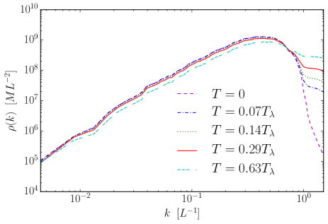
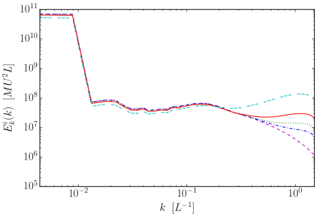
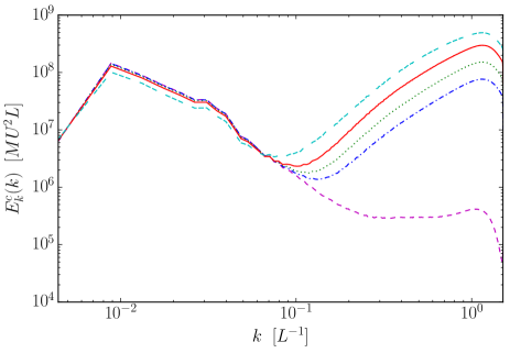
Figure 2: (Color online) From top to bottom, spectra of mass fluctuations, of the incompressible kinetic energy, and of the compressible kinetic energy, for several initial conditions of the GPE at different temperatures. All simulations have $N=1024$ linear spatial resolution.

One last aspect of the GPE dynamics of relevance for this work is the concept of helicity. In classical fluids the helicity is defined as

$$H=\int_{V}dV{\bm{v}}\cdot{\bm{\omega}},$$ (9)

where ${\bf\omega}$ stands for the vorticity field. Helicity is a measure of the mean alignment between velocity and vorticity (and thus, of the depletion of nonlinearities), of the topological complexity of vorticity field lines, as well as a measure of the departure of mirror-symmetry of the flow Moffatt (1969); Moffatt and Ricca (1992); Moffatt and Tsinober (1992); Moffatt (2014). In classical turbulence the presence of helicity in a turbulent flow can have multiple consequences, such as the depletion of the nonlinearities and energy transfers Kraichnan (1973), the slowing down of the onset of dissipation André and Lesieur (1977), and it can even affect the evolution of convective storms Lilly (1986). It has also been show that the helicity, just like the energy, develops a turbulent cascade where it is transferred from the larger to the smaller scales Brissaud et al. (1973). Moreover, the form of the cascade implies that it is a dual cascade, meaning that both energy and helicity have simultaneously non-zero transfer rates in the inertial range. In quantum fluids, Kelvin waves are helical and thus $H$ could in principle be used as a proxy to quantify the excitation of Kelvin waves at small scales. However, both ${\bf v}$ and ${\bf\omega}$ are singular along the vortex lines of a quantum fluid, where all the vorticity is concentrated. To overcome this problem, many authors have chosen to work with a definition of helicity based on its topological interpretation Scheeler et al. (2014). These geometric decompositions can result in zero net helicity Hänninen et al. (2016) but recover a classical non-zero value at large-scales Salman ; Kedia et al. (2017). Other authors have chosen to work with filtered fields Zuccher and Ricca (2015). Here we will use the regularized helicity introduced in Clark di Leoni et al. (2016), where the velocity field is regularized before being used to compute $H$. This method was shown to give results compatible with other methods in the literature to estimate the helicity of a quantum flow, and was used successfully to study helical quantum turbulence at zero temperature in massive numerical simulations in Clark di Leoni et al. (2017), where the existence of a dual cascade of energy and helicity was confirmed for the quantum case.

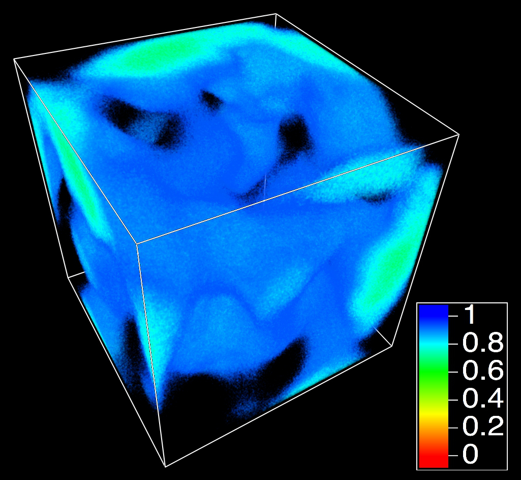
Figure 3: (Color online) Volume rendering of the density field for the simulation with $N=4096$ and $T=0.64T_{\lambda}$. Similar to the zero temperature ABC flow Clark di Leoni et al. (2017), large structures and regions of quiescencenot present in the initial conditions are spontaneously formed within the flow. At the large scales, the flow resembles the structure of a classical ABC flow. The possibility of seeing these large scale structures formed by the quantized vortices (the smallest structures in the flow) in such detail is in part due to the large scale separation, product of the high resolution used in the simulation. At low resolution there is not enough scale separation between the large scales and the thermal fluctuations for such a structures to develop.

II.2 The Stochastic Ginzburg Landau equation

The spatially truncated version of different conservative systems of partial differential equations can achive, after long time integration, states of thermodynamic equilibrium known as thermalized states where energy is equipartitioned among all the possible spatial modes Lee (1952); Kraichnan and Chen (1989). A common way to truncate a system is via a Galerkin projector. Given a Fourier series expansion of the wavefunction

$$\Psi({\bm{r}},t)=\sum^{\infty}_{k=-\infty}\hat{\Psi}_{\bm{k}}(t)e^{i{{\bm{k}}\cdot\bm{r}}},$$ (10)

where $\hat{\Psi}_{\bm{k}}$ are the Fourier coefficients and ${\bm{k}}$ are the wavevectors, the projector has the form

$${P}_{k_{G}}[\Psi({\bm{r}},t)]=\sum_{|k|\leq k_{G}}\hat{\Psi}_{\bm{k}}(t)e^{i{{\bm{k}}\cdot\bm{r}}}.$$ (11)

Applying it to Eq. (1) would give the so-called Fourier (or Galerkin) truncated version of the GPE.

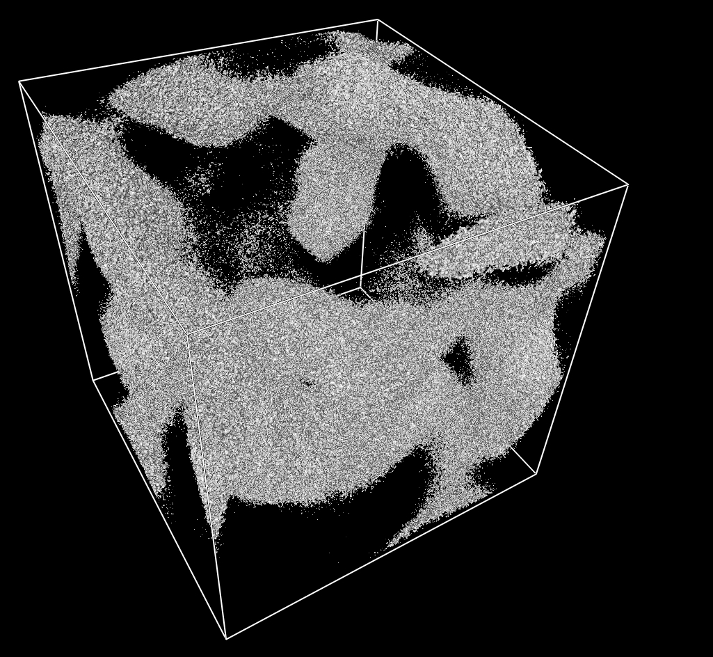
Figure 4: (Color online) Isosurfaces of the density field for the simulation with $N=4096$ and $T=0.64T_{\lambda}$. Contrary to the zero temperature case Clark di Leoni et al. (2017), it is not possible to discern individual vortices now. But their presence in the flow is still evident when looking at the fine-grain structures. Also, the formation of the vortex bundles observed in the zero temperature case is hampered in this case.

The studies of Davis et al. (2001) and of Connaughton et al. (2005) showed that if the Fourier truncated version of the GPE is integrated for long enough, the system indeed reaches a thermodynamic equilibrium. The statistical properties of this state are given by the microcanonical ensamble defined with fixed energy $E$, momentum ${\bf P}$, and number of particles $\mathcal{N}$. Moreover, if $E$ is varied, a phase transition akin to that of BECs can be observed, where the zero-wavenumber $A_{0}=\langle\Psi\rangle$ mode becomes equal to zero for finite $E$. But there are two problems with generating thermal states in this way. One is that the truncated GPE takes a very long time to converge to the equilibrium state, making it computationally expensive. The other is that the temperature is not easily accessed nor controlled in this way, given the complicated expression for the entropy in the microcanonical state of the the system. In order to overcome these problems, Krstulovic and Brachet (2011a, b) suggested using a Langevin process to generate grand-canonical states with distribution probability $\mathbb{P}_{\rm st}$ given by a Boltzmann weight $\mathbb{P}_{\rm st}=e^{-\beta F}/\mathcal{Z}$, where $\mathcal{Z}$ denotes the grand partition function and

$$F=E-\mu\mathcal{N}-{\bf W}\cdot{\bf P},$$ (12)

is a free energy with $\beta$ the inverse temperature, $\mu$ is the chemical potential, and ${\bf W}$ is related to the counterflow velocity. These grand-canonical states are faster to generate than microcanonical states, and give easy access and control of the temperature in the equilibrium.

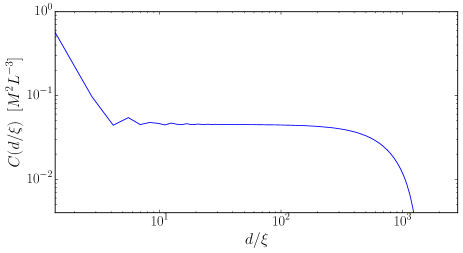
Figure 5: (Color online) Mass density correlation function $C(d)=\left<(\rho({\bf x}+d\hat{x})-\rho_{0})(\rho({\bf x})-\rho_{0})\right>$ for the simulation with $N=4096$ and $T=0.64T_{\lambda}$ at $t\approx 1$, with the displacement $d$ normalized in units of the healing length $\xi$. Note the slow decay of the correlation up to distances $\approx 10^{3}\xi$.

The Langevin process that generates these states has a Ginzburg-Landau equation of the type

$$\hbar\frac{\partial A_{\bf k}}{\partial t}=-\frac{\partial F}{\partial A^{*}_{\bf k}}+\sqrt{\frac{2\hbar}{\beta}}\hat{\xi}({\bf k},t),$$ (13)

$$\langle\xi({\bf r},t)\bar{\xi}({\bf r}^{\prime},t^{\prime})\rangle=\delta(t-t^{\prime})\delta({\bf r}-{\bf r}^{\prime}),$$ (14)

where $A_{\bf k}$ are the Fourier modes of the wavefunction, and $\hat{\xi}({\bf k},t)$ is the Fourier transform of the Gaussian delta-correlated noise $\xi({\bf r},t)$. In Krstulovic and Brachet (2011b) it is shown that the stationary probability of the solutions of Eq. (13) is indeed $\mathbb{P}_{\rm st}$. Thus, the grand-canonical states are simply generated by integrating the Langevin Eq. (13) in time until statistical convergence is obtained.

In physical space, the Langevin equation reads

$$\hbar\frac{\partial\Psi}{\partial t}= \left[\frac{\hbar^{2}}{2m}\nabla^{2}\Psi+\mu\Psi-g|\Psi|^{2}\Psi-i\hbar{\bf W}\cdot\nabla\Psi\right]$$

$$+\sqrt{\frac{2\hbar}{\beta}}\xi.$$ (15)

This equation will be referred to as the Stochastic Ginzburg-Landau equation (SGLE). The chemical potential $\mu$ controls the total number of particles $\mathcal{N}$. Different solutions obtained by varying $\beta$ will have different ratios of condensed fraction $|A_{0}|^{2}/\mathcal{N}=\mathcal{N}_{0}/\langle\mathcal{N}\rangle$, except below a critical $\beta$ (or, in terms of temperature, above the transition temperature $T_{\lambda}$) where this ratio will be equal to zero.

The thermal states obtained from the SGLE can then be fed to the GPE, in combination with an initial condition for the large-scale flow, to simulate a quantum turbulent flow at finite temperature. The total initial condition for the GPE $\Psi$ then has the form

$$\Psi=\Psi_{\mathrm{flow}}\times\Psi_{\mathrm{SGLE}},$$ (16)

where $\Psi_{\mathrm{flow}}$ is an initial wavefunction describing the flow, and $\Psi_{\mathrm{SGLE}}$ is a thermal solution of the SGLE which gives account of the occupation numbers of the different energy levels in the thermal state at a given temperature.

Although for simplicity the projector defined in Eq. (11) is not explicity written in Eqs. (1) and (15), in the following we will indeed solve the truncated versions of each equation. It is also worth noting that every time one solves a system of partial differential equations numerically, one is actually solving for truncated equations. Depending on the numerical method used for spatial discretization, the integration can preserve the conservation properties of the truncated system or not. The method used here, and described next, preserves all quantities conserved by the Galerkin truncated Eqs. (1) and (15) in the continuum-time case (i.e., before time discretization).

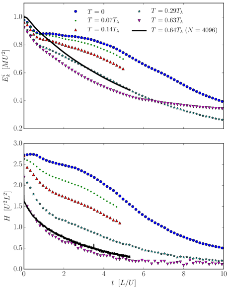
Figure 6: (Color online) Evolution of the incompressible kinetic energy (top) and of the helicity (bottom) as function of time at different temperatures. All simulations have $N=1024$ linear resolution, except the the one indicated with the solid black line which has $N=4096$. The early “inviscid-like” behavior seen at low temperature, in which energy and helicity remain approximately constant, is lost as the temperature is increased.

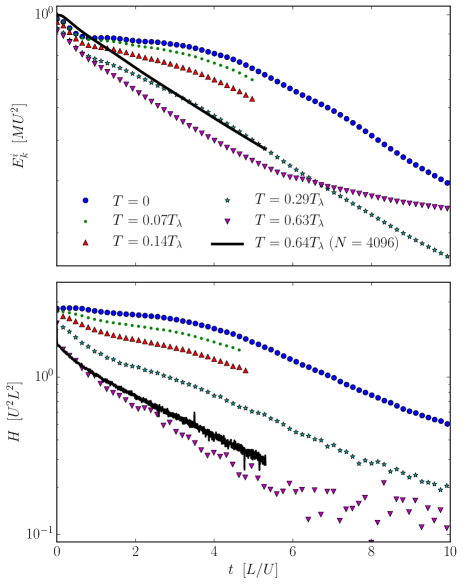
Figure 7: (Color online) Evolution of the incompressible kinetic energy (top) and of the helicity (bottom) as a function of time and at different temperatures in semi-logarithmic scale. All simulations have $N=1024$, except the one indicated with the solid black line which has $N=4096$. At the highest temperatures quantities decay exponentially in time.

II.3 Initial conditions and numerical simulations

To solve numerically Eqs. (1) and (15) in three dimensions we used GHOST Mininni et al. (2011), which uses a pseudospectral method combined with a fourth order Runge-Kutta scheme to solve Eq. (1), and an implicit Euler scheme to solve Eq. (15). Boundary conditions are periodic, each side of the simulation box is of size $2\pi L$ (where $L$ is a characteristic scale of the flow), and the “2/3 rule” is used for dealising. A hybrid OpenMP-MPI scheme is used for the parallelization. Multiple simulations were done at three different spatial resolutions $N^{3}$, with linear resolutions $N=128$, $N=1024$ and $N=4096$. In all cases, the speed of sound is chosen to be twice the characteristic flow velocity. For the simulation at the largest resolution ($N=4096$), a total of 8192 processors were used with 4096 MPI jobs and 2 threads per MPI job, and over 16 million CPU hours were used for the integration of this simulation.

All quantities are made dimensionless using a characteristic length, a speed, and a mass. Quantities with units can be determined at any time by doing $L=L^{\prime}/(2\pi)$, $U=c^{\prime}/2$, and $M=M^{\prime}/(2\pi)^{3}$, where $L^{\prime}$ is the characteristic length of the physical system, $c^{\prime}$ is the speed of sound, and $M^{\prime}$ is the fluid or gas mass (note all primed quantities have units). With this choice, the length of the simulation domain is equal to $2\pi L$, the speed of sound $c$ is equal to $2U$, and the mean density $\rho_{0}$ is equal to $1\,M/L^{3}$. The healing length $\xi$ is such that $k_{\max}\xi=1.5$, where $k_{\max}=N/3$ (in units of $1/L$) is the largest resolved wavenumber in each simulation (the equivalent of $k_{G}$ in Eq. (11)). In the highest resolved simulation, the healing length then is $\xi\approx 0.0011L$. As a referece, in superfluid ⁴He experiments the characteric system size is $L^{\prime}\approx 10^{-2}$ m, the speed of sound is $c^{\prime}\approx 230$ m/s, the fluid density is $\approx 125$ kg/m³ (thus $M^{\prime}\approx 1.25\times 10^{-4}$ kg), and the healing length is $\xi^{\prime}\approx 10^{-8}\,\textrm{m}\approx 10^{-6}L$ Barenghi et al. (2014). The insufficient scale separation of our highest resolved simulation (even with the massive resolution considered) is however much better suited for comparisons with BECs. In this case $L^{\prime}\approx 10^{-4}$ m, $c^{\prime}\approx 2\times 10^{-3}$ m/s, and $\xi\approx 5\times 10^{-7}\,\textrm{m}\approx 0.005L$ White et al. (2014). For the sake of simplicity, in the following all quantities are quoted using $L=M=U=1$, units can be added later using the procedure explained above. Finally, temperatures in the following will be always expressed explicitly in units of the transition temperature $T_{\lambda}$. More details on how units can be handled in GPE and SGLE simulations can be found in Nore et al. (1997b); Krstulovic and Brachet (2011a, b).

Simulations with $N=128$ and with $N=1024$ were performed at different temperatures, while only one simulation at a fixed temperature was performed at $N=4096$. All simulations were performed with no counterflow, so ${\bf W}$ in Eq. (15) is always set to zero, and the normal and superfluid components are in all cases in perfect coflow.

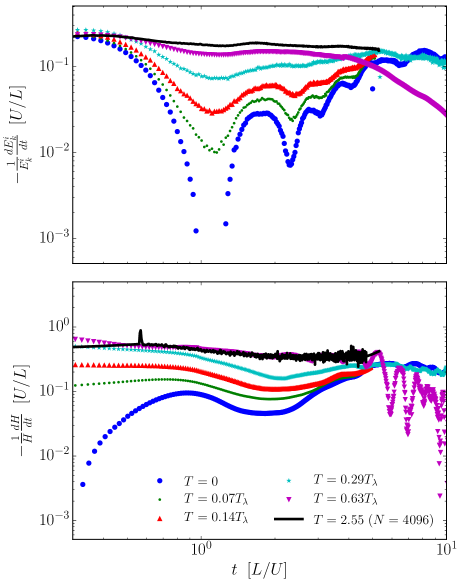
Figure 8: (Color online) Confirmation of exponential decay for the high temperature simulations, akin to that of a viscous classical fluid: incompressible kinetic energy exponential decay rate $-(1/E^{i}_{k})dE^{i}_{k}/dt$ for different temperatures in $N=1024$ runs (top), and same for the helicity $-(1/H)dH/dt$ (bottom). While simulations at low temperature display oscillations at early times and growth at late times, at the highest temperatures these quantities remain approximately constant for long times, allowing us to estimate an exponential decay rate.

In order to get a helical flow at large-scales, for the flow initial conditions $\Psi_{\mathrm{flow}}$ we used a superposition of two quantum Arnold-Beltrami-Childress (ABC) flows Clark di Leoni et al. (2017). The velocity field is a superposition of an ABC flow at $k=1$ and of an ABC flow at $k=2$: ${\bf v}_{\rm ABC}={\bf v}_{\rm ABC}^{(1)}+{\bf v}_{\rm ABC}^{(2)}$, with

$${\bf v}_{\rm ABC}^{(k)}= \left[B\cos(ky)+C\sin(kz)\right]{\bf i}+\left[C\cos(kz)+\right.$$ (17)

$$\left.A\sin(kx)\right]{\bf j}+\left[A\cos(kx)+B\sin(ky)\right]{\bf k}$$

with $(A,B,C)=(0.9,1,1.1)/\sqrt{3}$, and where ${\bf i}$, ${\bf j}$, and ${\bf k}$ are the three Cartesian vectors. The wavefunction that generates this flow after a Madelung transformation is obtained by the following procedure, detailed in Clark di Leoni et al. (2016). First, we set $\Psi_{\rm flow}=\Psi_{\rm ABC}^{(1)}\times\Psi_{\rm ABC}^{(2)}$, with $\Psi_{\rm ABC}^{(k)}=\Psi_{A,k}^{x,y,z}\times\Psi_{B,k}^{y,z,x}\times\Psi_{C,k}^{z,x,y}$, and with $\Psi_{A,k}^{x,y,z}=\exp\{i[A\sin(kx)\,m/\hbar]y+i[A\cos(kx)\,m/\hbar]z\}$, where $[a]$ stands for the nearest integer to $a$. In order to minimize the amount of energy in acoustic modes at the initial condition, we then evolve $\Psi_{\mathrm{flow}}$ using the advected real Ginzburg-Landau equation (ARGLE), whose stationary solutions are solutions of the GPE with minimal amount of phonons. The ARGLE explicitly reads

$$\partial_{t}\Psi= \frac{\hbar}{2m}\nabla^{2}\Psi+(\frac{g\rho_{0}}{m}-g|\Psi|^{2}-\frac{m{\bf v}_{\rm ABC}^{2}}{2\hbar})\Psi$$

$$-i{\bf v}_{\rm ABC}\cdot\nabla\Psi.$$ (18)

More information on the ARGLE can be found in Nore et al. (1997b), while the details of the quantum ABC flow are discussed in Clark di Leoni et al. (2016, 2017). The resulting flow has maximal helicity, and was used in Clark di Leoni et al. (2017) to study helical quantum turbulence at zero temperature.

Once $\Psi_{\mathrm{flow}}$ has been computed, we solve Eq. (15) to obtain a thermal solution at a given temperature, and finally we compute the initial conditions for the GPE using Eq. (16).

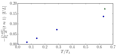
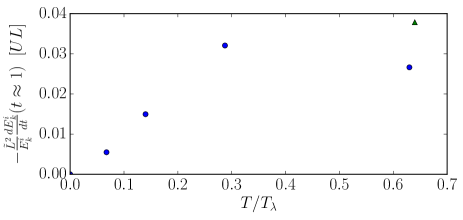
Figure 9: (Color online) Estimation of the effective viscosity from the energy decay rate, $\nu_{\textrm{eff}}=-(\tilde{L}^{2}/E^{i}_{k})dE^{i}_{k}/dt$ in the vicinity of $t\approx 1$, as a function of the temperature. Two choices for the characteristic scale are shown: the lengthscale of the initial ABC flow $\tilde{L}=L_{0}$ (top), and the correlation length of the incompressible velocity field $\tilde{L}=L_{i}$ in the vicinity of $t\approx 1$ (bottom). The (blue) circles indicate the simulations with $N=1024$, and the (green) triangle the simulation with $N=4096$.

III Numerical results

III.1 Temperature scans

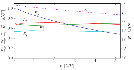
Figure 10: (Color online) Evolution of the total energy and its different components for the simulation with $T=0.64T_{\lambda}$ and $N=4096$.

In order to characterize the system we first perform a temperature scan solving the SGLE with the chemical potential $\mu$ adjusted to keep the total density $\rho_{0}=1$. In Fig. 1 we show the condensate fraction $\mathcal{N}_{0}/\langle\mathcal{N}\rangle$ (with $\mathcal{N}_{0}=|A_{0}|^{2}$) at late times in the evolution, as a function of the temperature $T$. As reported before in Krstulovic and Brachet (2011a, b), the typical behavior for second order transitions can be observed, with $\mathcal{N}_{0}/\langle\mathcal{N}\rangle\approx 0$ for $T>T_{\lambda}$, and $\mathcal{N}_{0}/\langle\mathcal{N}\rangle$ growing as in a phase transition for $T<T_{\lambda}$. The value of the critical temperature $T_{\lambda}$ was determined from this analysis. The scans were performed at two different linear resolutions $N=128$ and $N=1024$. The results from both coincide, showing the simulations are well converged. Also shown in the figure is the usual prediction for the condensate fraction coming from ideal BEC theory Pathria and Beale (1996) where $\mathcal{N}_{0}/\langle\mathcal{N}\rangle=1-(T/T_{\lambda})^{3/2}$. This prediction does not match our results exactly as it is derived for non-interacting bosons, which is not our case. Nonetheless, the behaviors are similar.

As explained above, these thermal states were coupled to solutions of the ARGL to generate initial conditions for the GPE at different temperatures. In Fig. 2 we show the spectrum of the mass fluctuations $\rho(k)$ of the initial condition for five different temperatures, as well as the incompressible kinetic energy spectrum $E_{k}^{i}(k)$, and the compressible kinetic energy spectrum $E_{k}^{c}(k)$. In all cases, the increasing amplitude of high wavenumber (small scale) modes as $T$ is increased (but specially in $E_{k}^{c}(k)$, associated with phonon excitations) accounts for the increasing thermal effects. Note however that the low wavenumber (large scale) spectrum of $E_{k}^{i}(k)$, associated with the initial ABC flow, remains largely unaffected by the thermal fluctuations, a result of the sufficient scale separation in these runs.

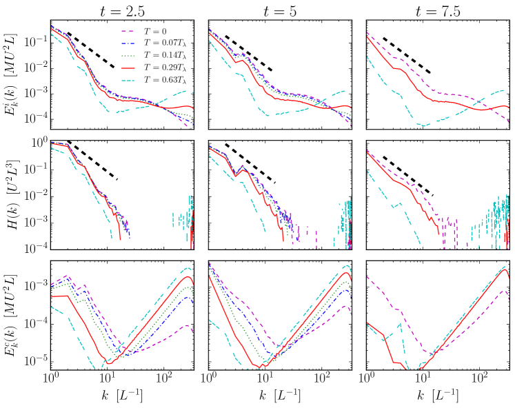
Figure 11: (Color online) Spectra of incompressible kinetic energy, helicity, and compressible kinetic energy at different temperatures and at different times. All simulations have $N=1024$ linear resolution. The thick dashed line indicates $k^{-5/3}$ scaling, predicted for the dual cascade of energy and helicity Brissaud et al. (1973), and previously observed in zero temperature simulations Clark di Leoni et al. (2017). This scaling is compatible with the simulations at at low temperatures, but it is lost once the temperature is increased and viscous effects become strong enough.

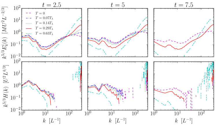
Figure 12: (Color online) Compensated version of the incompressible kinetic energy and helicity spectra shown in Fig. 11. As seen in the figure, only at the smaller temperatures some range of wave numbers compatible with $k^{-5/3}$ scaling (i.e., an approximately flat compensated spectrum) is recovered.

III.2 Dynamical evolution

We now focus on understanding finite temperature effects on the evolution of the GPE. We thus show results from six different simulations. Five of them were done at a linear resolution of $N=1024$, with temperatures ranging from zero to $T=0.63T_{\lambda}$, while the sixth simulation was performed at a linear resolution of $N=4096$ and at $T=0.64T_{\lambda}$.

III.2.1 Large-scale flow structure

We begin by showing two visualizations of the density field for the simulation with $N=4096$ and $T=0.64T_{\lambda}$ at time $t\approx 1$. In Fig. 3, a volumetric rendering of mass density is shown using VAPOR Clyne et al. (2007). Similarly to the zero temperature quantum ABC flow Clark di Leoni et al. (2017), large vortex bundles are formed within the flow, and regions of quiescence (with almost no vorticity) appear. At the larger scales the structure of the flow looks similar to that of a classical ABC flow, as expected. Moreover, although the thermal fluctuations blur the small scales, the large scale flow is clearly discernible. In Fig. 4 isosurfaces of the density field are shown. As in Fig. 3, and contrary to the zero temperature case where it is easy to spot individual vortices (see Clark di Leoni et al. (2017)), the thermal noise lumps the vortices inside the bundles, making it difficult to discern individual structures from visual inspection, although traces of their presence are evident.

To further confirm the coexistence of large-scale correlations (associated with the flow) with small-scale thermal fluctuations and vortices, we show in Fig. 5 the spatial correlation function of mass density fluctuations

$$C(d)=\left<(\rho({\bf x}+d\hat{x})-\rho_{0})(\rho({\bf x})-\rho_{0})\right>/\rho_{0}^{2},$$ (19)

for the simulation with $N=4096$ and $T=0.64T_{\lambda}$ at time $t\approx 1$, where $d$ is the spatial displacement (which in Fig. 5 is normalized in units of the healing length $\xi$). The function $C(d)$ is also proportional, by the Wiener-Khinchin theorem, to the Fourier transform of the internal energy spectrum. Note $C(d)$ decays rapidly with $d/\xi$ in a distance proportional to the vortex core size, thus further confirming the presence of quantized vortices in the flow. Then, $C(d)$ remains almost constant up to very long-range distances ($d\approx 10^{3}\xi$), confirming the presence of a large-scale structure in the system.

III.2.2 Energy and helicity decay

In the zero temperature case nonlinear interactions of Kelvin waves lead to the emission of phonons L’vov and Nazarenko (2010); Vinen and Niemela (2002), which deplete the incompressible kinetic energy Nore et al. (1997b) and the helicity Clark di Leoni et al. (2017). The presence of thermal noise adds a new depletion mechanism. In order to study it, we show in Figs. 6 and 7 the evolution of the incompressible kinetic energy $E^{i}_{k}$ and of the helicity $H$ for five different temperatures, in linear and in semi-logarithmic scales respectively.

As expected, for all temperatures both $E^{i}_{k}$ and $H$ decay in time. At very early times a short transient can be seen (due to the system correcting frustration effects coming from the initial conditions), after which the different dynamical mechanisms come into play. This transient is similar for all the runs, and almost independent of the temperature. After this transient, at low temperatures both the incompressible energy and the helicity decay very slowly or remain approximately constant (see in particular the case with $T=0$ in Fig. 7), up until $t\approx 3$. This is similar to what is observed in freely decaying classical turbulence: in that case the early “inviscid-like” phase corresponds to the build up of the turbulent cascade while dissipation remains negligible, and which (in the classical case) ends when small scale excitations reach the viscous dissipation scale. In classical turbulent flows, the presence of helicity is known to extend the duration of this “inviscid-like” phase (see, e.g., Teitelbaum and Mininni and references therein). As explained in (Clark di Leoni et al., 2017), in the quantum case and for $T$ close to zero this inviscid phase corresponds to the time during which vortices interact and the Kelvin wave cascade builds up, so after $t\approx 4$ the emission of phonons becomes prominent and the incompressible kinetic energy and the helicity start being depleted. Note that during this phase both energy and helicity are transferred towards smallers scales, as will be confirmed later by the energy and helicity spectra.

Unlike the simulations at low temperature, the simulations at the highest temperatures go directly from the short initial transient to a seemingly exponential decay, without an inviscid-like phase in between (see Fig. 7). At late times ($t>6$), all simulations show similar exponential decay rates (see Fig. 7) as a significant fraction of the energy has already thermalized, with the exception of the simulation with $T=0.64T_{\lambda}$ and $N=1024$, which has a higher initial temperature and thus can reach a thermal equilibrum faster. The exponential decay observed in these runs is reminiscent of what is observed in the free decay of low Reynolds classical flows. To further verify this we show estimations of the exponential decay rates $-(1/E^{i}_{k})dE^{i}_{k}/dt$ and $-(1/H)dH/dt$ in Fig. 8. For the higher temperatures these magnitudes become close to constant for long periods of time, confirming an exponential decay. This is not the case for the lower temperatures, where oscillations and a late growth of these quantities are present at all times. Moreover, the exponential decay behavior at high temperatures is compatible with weak nonlinearities and can be used, as explained below, to estimate an effective eddy viscosity of the flow by assuming a governing equation for the velocity of the Stokes form, $\partial{\bf v}/\partial t\approx\nu_{\textrm{eff}}\nabla^{2}{\bf v}$.

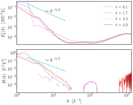
Figure 13: (Color online) Spectra of the incompressible kinetic energy and of the helicity at $T=0.64T_{\lambda}$ in the simulation with $N=4096$ at different times. A turbulent scaling law is shown as a reference. Although nonlinear excitations develop, the range of scales compatible with the turbulent scaling is short and at late times the spectrum decays rapidly.

So far, these results indicate several things: The effects of the thermal states generated with the SGLE upon the quantum turbulent flow can be modeled, at least for global quantities and in the simplest scenario, using an effective viscous dissipation. This effect can be, at the highest temperatures considered, strong enough (even at the highest resolution) that nonlinear interactions and Kelvin wave turbulence cannot fully develop, such that (pseudo) viscous effects dominate the dynamics. As observed from Fig. 8, the rate of change of the energy at zero temperature is almost negligible at $t\approx 1$, but increases and becomes considerable in the other cases. Thus, we can draw from this fact to construct anzats for the effective viscosity as a function of temperature. In a freely decaying classical flow an eddy viscosity can be estimated as $\nu_{\textrm{eff}}=-(\tilde{L}^{2}/E^{i}_{k})dE^{i}_{k}/dt$, where $\tilde{L}$ is some large-scale correlation length. Here we have several choices for a characteristic length $\tilde{L}$: a fixed length $L_{0}$ given by the length scale of the large-scale flow at $t=0$, the integral scale (i.e., the correlation length) of the incompressible velocity field

$$L_{i}=\frac{2\pi}{E_{k}^{i}}\int{\frac{E_{k}^{i}(k)}{k}dk},$$ (20)

(where $E_{k}^{i}(k)$ is the spectrum of the incompressible kinetic energy), the intervortex distance $\ell$, or the healing length $\xi$. We verified that the behavior with temperature of $\nu_{\textrm{eff}}$ with all these choices for $\tilde{L}$ is qualitatively similar, except for a prefactor, and thus show in Fig. 9 two estimations of $\nu_{\textrm{eff}}$ based on large-scale correlation lengths: the fixed length $L_{0}$ and the integral length $L_{i}$. The viscosity estimates are close to zero for $T=0$, grow linearly with temperature up to $T/T_{\lambda}\approx 0.3$, and then either keep growing at a lower rate or decrease for larger temperatures, depending on the choice of $L$. Moreover, the estimations of $\nu_{\textrm{eff}}$ for the $N=1024$ and the $4096$ runs at the highest temperature are similar.

These results can be interpreted as follows. The viscosity of the normal fluid $\nu_{n}$ can be expected to be proportional to mean free path $\lambda_{m}$ times the sound velocity, i.e., $\nu_{n}\sim\lambda_{m}c$. When we increase the resolution fixing $\xi k_{\rm max}$ (as done here), $c$, and the temperature $T$, the mean free path depending only on the temperature is constant (in units of $\xi$), i.e.,

$$\lambda_{m}\sim\xi f(T/T_{\lambda}),$$ (21)

where $f(T/T_{\lambda})$ is a dimensionless function. Therefore $\nu_{n}$ should scale as the inverse of the spatial resolution, $\nu_{n}\sim 1/N$. But this argument holds as long as the mean free path is smaller than the box size, $\lambda_{m}<2\pi$, while the mean free path diverges when $T\to 0$. Thus, at a given temperature the viscosity of the normal fluid should first remain constant with resolution, and then after a certain critical resolution go to zero as $1/N$. This is for the normal fluid alone, and its contribution to the total flow should scale as $\rho_{n}/\rho\sim T$. Thus, we can expect an effective viscosity measured on the total fluid to scale as

$$\nu_{\rm eff}\sim\nu_{n}\rho_{n}/\rho\sim\nu_{n}T/T_{\lambda},$$ (22)

which should first grow like $T$ and then decrease when the mean free path becomes less than the box size. Further confirmation of this scaling would require a direct measure of the mean free path; we discuss possible methods to achieve this goal in the conclusions.

Finally, it is important to note that, as in the zero temperature case, the Galerking truncated GPE conserves the total energy, and that our spatial discretization method is also conservative (although time discretization introduces new errors as discussed next). So, while the incompressible kinetic energy is depleted, the other components of the energy can be expected to grow. As an illustration, the evolution of the total energy, the incompressible kinetic energy, the compressible kinetic energy, the quantum energy, and the potential energy for the simulation with $N=4096$ and $T=T0.64T_{\lambda}$ is shown in Fig. 10. Note a fraction of the total energy is indeed lost due to numerical errors, resulting from the fact that the great cost of doing such a high resolution simulation did not allow us to use a very small time step. Nonetheless, energy is conserved up to 95% when $t\approx 1$ (which is when most of the physics we are interested occurs) and up to 82% at the very end of the simulation.

III.2.3 Spatial spectra

Finally, we study the effect of temperature on the evolution of the spatial spectra of the two components of the kinetic energy (compressible and incompressible), and of the helicity. This should give further confirmation that for large enough temperatures, the nonlinear cascade of energy and of helicity is strongly arrested. The results for the simulations with $N=1024$ are shown in Fig. 11 (with compensated versions of the spectra shown in Fig. 12), while the results for the simulation with $N=4096$ are shown in Fig. 13. Note that the compensated spectra stemming from the simulations with $N=1024$ shown in Fig. 12 are expected to be flat in regions that follow Kolmogorov-like scaling; animations showing the evolution of each spectra can be also found in SI .

While, as shown in Fig. 2, the initial spectra at small wavenumbers (large scales) are relatively similar for all temperatures, differences can already be seen in Fig. 11 at $t=2.5$ for the simulations at different temperatures. In particular, the simulations with the largest temperatures have less power at small wavenumbers (for all quantities $E_{k}^{i}$, $H$, and $E_{k}^{c}$), and more power at large wavenumbers (specially for $E_{k}^{c}$), as can be expected from the larger thermal fluctuations. As the flow evolves and nonlinear interactions take place (see the spectra at $t=5$), the low temperature simulations develop a range of wavenumbers compatible with a Frisch-Brissaud dual cascade of energy and of helicity towards small scales Brissaud et al. (1973) (which corresponds to Kolmogorov-like scaling for both spectra), previously observed in zero temperature simulations Clark di Leoni et al. (2017). However, the simulations with the highest temperatures do not develop a broad spectrum, and although excitations grow at intermediate and at small wavenumbers in $E_{k}^{i}(k)$ and $H(k)$, the spectra drops faster confirming the effect of damping discussed in the previous section, and in agreement with the effect expected for a large effective viscosity. The compensated spectra shown in Fig. 12 confirm this. The $N=4096$ simulation (see Fig. 13) also shows this damped behavior, and as estimated from the results in Fig. 9 has an effective viscosity of the same order as the simulation with $N=1024$ at a similar temperature.

All spectra at all temperatures have a pronounced change (or knee) at around $k\approx 10$. At low temperatures, this bump (which in the case of the spectrum of $E_{k}^{i}$ is followed by a range of wavenumbers with decreasing amplitude as $k$ increases) can be associated with a bottleneck produced by the Kelvin wave cascade at scales smaller than the mean intervortex distance Clark di Leoni et al. (2017). This is seen more clearly in the compressible kinetic energy spectra. For the simulations at the highest temperatures this second range is swallowed up by the presence of the thermalized modes. As it can be expected, the flat portion of the spectra between the cascading part at small wavenumers and the thermalized part at large wavenumbers is wider in the $N=4096$ (Fig. 13) simulation compared to the ones at $N=1024$ (Fig. 11). The spectra of the helicity fluctuate around zero with fast changes in sign above this wavenumber in all cases, a result of the depletion of helicity by phonons (as the spectra are plotted in logarithmic scale only positive values are shown, the missing parts correspond to the negative values). The spectrum of compressible kinetic energy grows as $\sim k^{2}$, which can be expected for a thermalized state (and its amplitude increases with increasing temperature).

IV Conclusions

Modeling quantum flows at nonzero temperatures is key to understand recent experimental results of quantum turbulence. However, models for quantum flows at finite temperature are limited, sometimes derived from phenomenological models, in other cases obtained from coarse approximations, and in many cases their dynamics have not been fully characterized. Here we presented a study of helical quantum turbulence at various temperatures using very large resolution simulations and a model based on the Gross-Pitaevskii equation with thermal states generated by the Stochastic Guinzburg-Landau equation.

Our results show that in this model, under the presence of thermal noise, a quantum flow can behave as a viscous classical flow, with exponential decay of the incompressible kinetic energy and of the helicity. A smooth transition between the behavior at zero temperatures and at large temperatures (for temperatures lower than the critical) was reported. Moreover, the (pseudo) viscous effects can strongly quench the formation of a turbulent cascade, even at the largest spatial resolution considered. However, when the temperature is not too high, a dual cascade of energy and of helicity (as also observed in classical turbulence and in quantum flows at zero temperature) can be reobtained.

We presented a phenomenological estimation of the effective viscosity in this model, which shows linear scaling with increasing temperature, and a saturation for very high temperatures. An argument based on the mean free path accounts for this behavior, and opens the door to better estimations of the effective viscosity by measuring directly this lengthscale. This can be done by studying the spatio-temporal spectrum of the flow as a function of the temperature, which gives access to the spectrum of phonons in the system Clark di Leoni et al. (2015). However, as computation of this spectrum is computationally intensive, it can only be done at lower resolutions or using a different flow configuration, and is thus left for future work.