Exciton-phonon cooperative mechanism of the triple-$\bm{q}$ charge-density-wave
and antiferroelectric electron polarization in TiSe₂

Abstract

We investigate the microscopic mechanisms of the charge-density-wave (CDW) formation in a monolayer TiSe₂ using a realistic multiorbital $d$-$p$ model with electron-phonon coupling and intersite Coulomb (excitonic) interactions. First, we estimate the tight-binding bands of Ti $3d$ and Se $4p$ orbitals in the monolayer TiSe₂ on the basis of the first-principles band-structure calculations. We thereby show orbital textures of the undistorted band structure near the Fermi level. Next, we derive the electron-phonon coupling using the tight-binding approximation and show that the softening occurs in the transverse phonon mode at the M point of the Brillouin zone. The stability of the triple-$\bm{q}$ CDW state is thus examined to show that the transverse phonon modes at the M₁, M₂, and M₃ points are frozen simultaneously. Then, we introduce the intersite Coulomb interactions between the nearest-neighbor Ti and Se atoms that lead to the excitonic instability between the valence Se $4p$ and conduction Ti $3d$ bands. Treating the intersite Coulomb interactions in the mean-field approximation, we show that the electron-phonon and excitonic interactions cooperatively stabilize the triple-$\bm{q}$ CDW state in TiSe₂. We also calculate a single-particle spectrum in the CDW state and reproduce the band folding spectra observed in photoemission spectroscopies. Finally, to clarify the nature of the CDW state, we examine the electronic charge density distribution and show that the CDW state in TiSe₂ is of a bond-type and induces a vortex-like antiferroelectric polarization in the kagomé network of Ti atoms.

I Introduction

Transition-metal dichalcogenides (TMDs) Wilson and Yoffe (1969); Chhowalla et al. (2013) are representative materials that show the charge-density-wave (CDW) states Motizuki (1986); Rossnagel (2011). The majority of the group-IV (Ti, Zr, Hf) TMDs are simple $d^{0}$ semiconductors, in which the Fermi level is located between the valence chalcogen $p$ and conduction transition-metal $d$ bands Chhowalla et al. (2013). However, 1$T$-TiSe₂, one of the group IV TMDs, is either a slightly band-overlap semimetal or a small band-gap semiconductor Zunger and Freeman (1978); Fang et al. (1997), which is the only material that shows the CDW transition among this group Woo et al. (1976); Di Salvo et al. (1976); Holt et al. (2001). Thus, in contrast to the conventional (nesting induced) CDWs in low-dimensional solids Grüner (1988, 2000) or to the CDWs in the $d^{1}$ TMDs Wilson et al. (1974, 1975), a peculiar mechanism of the CDW formation should be expected in the $d^{0}$ TMD, 1$T$-TiSe₂. Furthermore, in 1$T$-TiSe₂, it is known that the emergence of superconductivity (SC) with melting of the CDW is caused by intercalation Morosan et al. (2006, 2007); Li et al. (2007a); Morosan et al. (2010); Giang et al. (2010); Luo et al. (2016a); Song et al. (2016); Sato et al. (2017), applying pressures Kusmartseva et al. (2009); Joe et al. (2014), or carrier doping Li et al. (2016); Luo et al. (2016b). Therefore, clarifying the origin of the CDW is significant also for the elucidation of the mechanism of its SC.

Because the electronic band structure of TiSe₂ is located near the semimetal-semiconductor phase boundary, its CDW phase has been investigated as a candidate for the excitonic phase Wilson (1977); Traum et al. (1978). This phase is also referred to as an excitonic insulator state, where a spontaneous hybridization between the orthogonal valence and conduction bands occurs by the interband Coulomb interaction to open the band gap Keldysh and Kopeav (1965); Des Cloizeaux (1965); Jérome et al. (1967); Kohn (1967); Halperin and Rice (1968a, b). Studies of the excitonic phases have recently been developed in terms of localized orbital models appropriate for strongly correlated electron systems Seki et al. (2011); Kaneko et al. (2012); Ejima et al. (2014); Kuneš and Augustinský (2014a, b); Kuneš (2015); Nasu et al. (2016) and adaptation of the excitonic theory for real materials is desired. Because TiSe₂ as well as another candidate material Ta₂NiSe₅ Di Salvo et al. (1986); Wakisaka et al. (2009); KTK ; Seki et al. (2014); Yamada et al. (2016); Lu et al. (2017) are among transition-metal compounds, the orbital textures and Coulomb interactions between the local orbitals may be essential factors in considering their electronic properties. In fact, photoemission spectroscopies and related theoretical analyses have suggested that the excitonic mechanism can be applied for the CDW formation in TiSe₂ Pillo et al. (2000); Kidd et al. (2002); Cercellier et al. (2007); Li et al. (2007b); Qian et al. (2007); Zhao et al. (2007); Monney et al. (2009, 2010a, 2010b); May et al. (2011); Cazzaniga et al. (2012); Monney et al. (2012a, b, 2015).

The phononic mechanism (or the band-type Jahn-Teller mechanism) of the CDW formation has also been suggested Hughes (1977); White and Lucovsky (1977), where the CDW transition around $T=200$ K associated with the 2$\times$2$\times$2 periodic lattice displacement (PLD) Woo et al. (1976); Di Salvo et al. (1976); Holt et al. (2001) is essentially explained by the electron-phonon coupling. Microscopic theory of the phononic mechanism was developed by Motizuki and coworkers Yoshida and Motizuki (1980); Takaoka and Motizuki (1980); Motizuki et al. (1981a, b); Suzuki et al. (1984, 1985); Motizuki (1986) using the realistic crystal and electronic structures of 1$T$-TiSe₂. The realization of the 2$\times$2$\times$2 PLD was thereby explained quantitatively. Recent first-principles phonon calculations Calandra and Mauri (2011); Bianco et al. (2015); Duong et al. (2015); Fu et al. (2016); Singh et al. (2017); Hellgren et al. (2017) have also predicted consistent results with those of Motizuki et al.. Experimentally, the lattice dynamics and phonon softening corresponding to the superlattice formation have been studied by the Raman and infrared spectroscopy Holy et al. (1977); Sugai et al. (1980); Snow et al. (2003); Barath et al. (2008); Goli et al. (2012); Duong et al. (2017), as well as by the inelastic neutron and x-ray scattering experiments Stirling et al. (1976); Wakabayashi et al. (1978); Jaswal (1979); Weber et al. (2011); Maschek et al. (2016).

Thus the two different driving forces for the CDW formation, i.e., excitonic and phononic forces, have been suggested in TiSe₂, of which the determination is still controversial. Recent theoretical studies have also suggested that the electron-phonon coupling and excitonic interactions cooperatively stabilize the CDW state van Wezel et al. (2010); Zenker et al. (2013); Watanabe et al. (2015); Kaneko et al. (2015). These studies, however, do not assume the electron-phonon couplings with realistic phonon modes corresponding to the experimentally observed PLD. The studies by Motizuki et al. and first-principles phonon calculations, on the other hand, do not assume the excitonic ordering induced by the interband Coulomb interaction. In addition, local orbital textures of the CDW in TiSe₂ have not been investigated in detail. Therefore, to elucidate the origin and local structure of the CDW and PLD in TiSe₂, it is highly desired to develop a quantitative microscopic theory based on a realistic model that reflects the actual crystal and electronic orbital structures in TiSe₂, taking into account both the phononic and excitonic interactions.

Motivated by these developments in the field, here we investigate the microscopic mechanisms and electronic structures of the CDW phase in a monolayer TiSe₂ on the basis of the realistic multi-orbital $d$-$p$ model, where both the electron-phonon coupling and intersite Coulomb interactions are taken into account. We thereby clarify both the phononic and excitonic mechanisms of the CDW transition. Although we assume the monolayer TiSe₂ for simplicity, our theoretical study will provide helpful interpretations of recent experiments on monolayer as well as few-layer TiSe₂ Peng et al. (2015); Chen et al. (2015); Sugawara et al. (2016); Chen et al. (2016); Fang et al. (2017).

First, we construct the tight-binding bands of the Ti 3$d$ and Se 4$p$ orbitals in the monolayer TiSe₂ using the first-principles band-structure calculations. From the obtained energy bands in the undistorted crystal structure, we show orbital components of the bands and deduce the effective electronic structure near the Fermi level. Next, we derive the electron-phonon coupling in the tight-binding approximation for the transverse phonon modes, of which the softening has been observed experimentally Holt et al. (2001). Then, taking into account the electron-phonon coupling only, we show the softening of the transverse phonon mode at the M point of the Brillouin zone (BZ). We thus discuss the instability toward the triple-$\bm{q}$ CDW state, where the transverse phonon modes at the M₁, M₂, and M₃ points are frozen simultaneously. Furthermore, we introduce the intersite Coulomb interaction between the nearest-neighbor Ti and Se atoms that induces the excitonic instability between the valence Se 4$p$ and conduction Ti 3$d$ bands. We investigate the roles of the excitonic interaction in the triple-$\bm{q}$ CDW state using the mean-field approximation for the intersite Coulomb interactions. We thus show that the electron-phonon and excitonic interactions cooperatively stabilize the triple-$\bm{q}$ CDW state in TiSe₂. We can also show that the calculated single-particle spectrum in the CDW state can reproduce the band folding spectrum observed in photoemission spectroscopies. Finally, we examine the nature of the CDW state by calculating the change in the electron density distribution and predict that the CDW state in TiSe₂ is of a bond-centered-type, rather than a site-centered-type, and induces a vortex-like antiferroelectric polarization in the kagomé network of Ti atoms.

The rest of this paper is organized as follows. In Sec. II, we derive the effective eleven-orbital $d$-$p$ model for the monolayer TiSe₂ taking into account both the electron-phonon coupling and intersite Coulomb interactions. In Sec. III, we show the effective electronic structure near the Fermi level in the undistorted crystal structure. In Sec. IV, we present the phonon softening and instability toward the triple-$\bm{q}$ CDW state without taking into account the intersite Coulomb interactions. In Sec. V, we briefly review the mean-field approximation for the excitonic ordering and discuss the roles of the Coulomb interaction for the triple-$\bm{q}$ CDW in TiSe₂. In Sec. VI, we show the single-particle spectrum and charge density distribution in the CDW state. Discussions and summary are given in Sec. VII. Details of the calculations are provided in Appendices A–E.

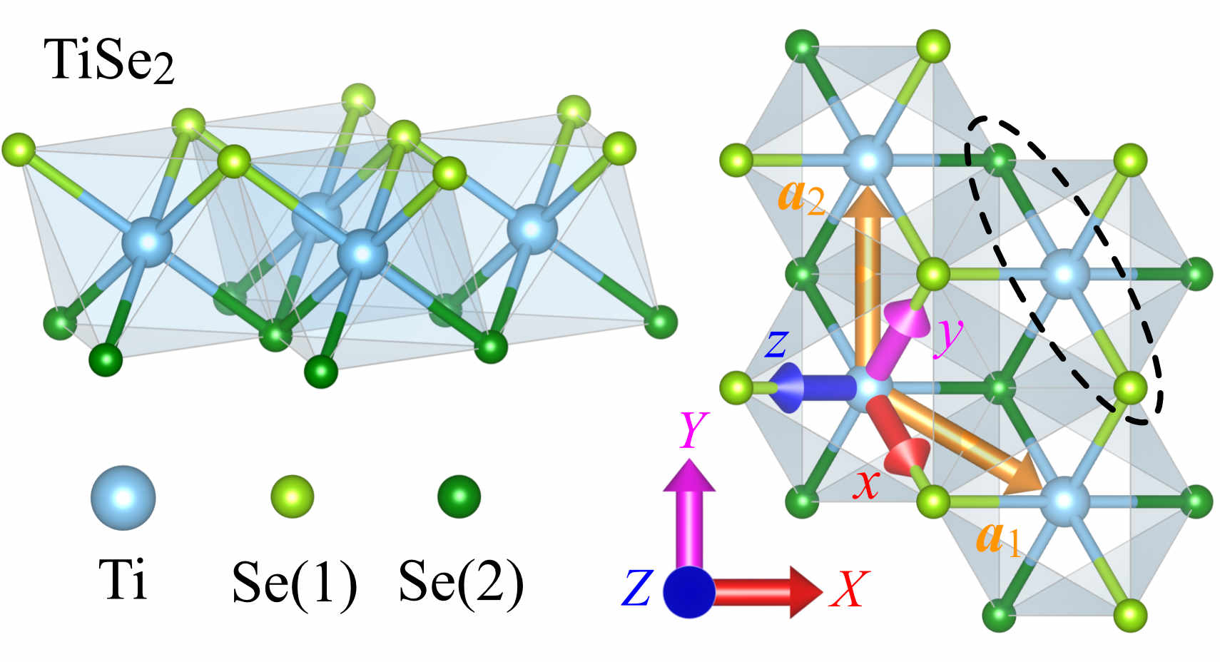
Figure 1: Schematic representations of the crystal structure of the monolayer TiSe₂. $X$-$Y$-$Z$ are the global coordinate axes and $x$-$y$-$z$ are the local coordinate axes in the TiSe₆ octahedron. Dashed ellipse is the unit cell taken in this paper. $\bm{a}_{1}$ and $\bm{a}_{2}$ are the primitive translation vectors.

II Model

First, let us construct the effective eleven-orbital $d$-$p$ model for the monolayer TiSe₂ taking into account the electron-phonon coupling and interband Coulomb interactions. The model enables us to consider both the phononic and excitonic mechanisms of the CDW transition. The crystal structure, tight-binding bands, electron-phonon coupling, and Coulomb interactions in TiSe₂ are discussed in the following subsections.

II.1 Crystal structure

The crystal structure of the monolayer 1$T$-TiSe₂ is illustrated in Fig. 1 . We assume the lattice constant $a=3.54$ Å Riekel (1976) and use the primitive translation vectors $\bm{a}_{1}=(\sqrt{3}a/2,-a/2)$ and $\bm{a}_{2}=(0,a)$ shown in Fig. 1. The unit cell contains one Ti ion and two Se ions, Se(1) and Se(2). The position of the Ti and Se ions in the unit cell are $\bm{\tau}_{\rm Ti}=(0,0,0)$ and $\bm{\tau}_{\rm Se1}=-\bm{\tau}_{\rm Se2}=(a/2\sqrt{3},-a/2,z_{\rm Se})$ with $z_{\rm Se}=1.552$ Å, where we apply the atomic position optimization in the WIEN2k code Blaha et al. (2001) to determine $z_{\rm Se}$ . We also illustrate the BZ of the monolayer TiSe₂ in Fig. 2, where the reciprocal primitive vectors are given by $\bm{b}_{1}=(4\pi/\sqrt{3}a,0)$ and $\bm{b}_{2}=(2\pi/\sqrt{3}a,2\pi/a)$.

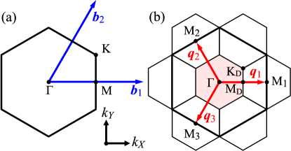
Figure 2: (a) The BZ of the monolayer TiSe₂, where $\bm{b}_{1}$ and $\bm{b}_{2}$ are the reciprocal primitive vectors. (b) Three M-points and reduced BZ (RBZ). $\bm{q}_{1}$, $\bm{q}_{2}$, and $\bm{q}_{3}$ corresponding to the modulation wave vectors of the CDW in TiSe₂. Red shaded area indicates the RBZ in the 2$\times$2 superlattice structure.

II.2 Tight-binding bands

We use the energy bands in the tight-binding (TB) approximation as a noninteracting band structure. The Hamiltonian of the TB bands is given by

$$\mathcal{H}_{e}=\sum_{\bm{k}}\sum_{\mu\ell,\nu m}t_{\mu\ell,\nu m}(\bm{k})c^{{\dagger}}_{\bm{k},\mu\ell}c_{\bm{k},\nu m},$$ (1)

where $c^{({\dagger})}_{\bm{k},\mu\ell}$ is the annihilation (creation) operator of an electron in orbital $\ell$ of atom $\mu$ at momentum $\bm{k}$. We do not write the spin index explicitly in this paper. $t_{\mu\ell,\nu m}(\bm{k})$ is the Fourier transform of the transfer integral

$$t_{\mu\ell,\nu m}(\bm{k})=\sum_{\bm{R}_{n}}t_{\mu\ell,\nu m}(\bm{R}_{n})e^{-i\bm{k}\cdot\bm{R}_{n}}.$$ (2)

$t_{\mu\ell,\nu m}(\bm{R}_{n})$ is the transfer integral between the atomic orbitals $\mu\ell$ and $\nu m$ at $\bm{R}_{n}=n_{1}\bm{a}_{1}+n_{2}\bm{a}_{2}$, where $n_{1}$ and $n_{2}$ are integers. The energy levels of the atomic orbitals are given by $t_{\mu\ell,\mu\ell}(\bm{R}_{n}=\bm{0})=\varepsilon_{\mu\ell}$.

From the first-principles band calculations Zunger and Freeman (1978); Fang et al. (1997), it is known that the band structure of TiSe₂ is given by six bands based on the Se 4$p$ orbitals below the Fermi level and five bands based on the Ti 3$d$ orbitals above the Fermi level. Therefore we consider the total eleven orbitals from the five 3$d$ orbitals in the Ti atom and three 4$p$ orbitals in the Se(1) and Se(2) atoms. A TiSe₆ octahedron has the $D_{3d}$ point-group symmetry and therefore we define the local coordinate axes $x$-$y$-$z$ from the global coordinate axes $X$-$Y$-$Z$ using the rotational transformation Kamimura et al. (1969)

$$\left(\begin{array}[]{c}x\\ y\\ z\end{array}\right)=\left(\begin{array}[]{r r r}{1}/{\sqrt{6}}&-{1}/{\sqrt{2}}&{1}/{\sqrt{3}}\\ {1}/{\sqrt{6}}&{1}/{\sqrt{2}}&{1}/{\sqrt{3}}\\ -{2}/{\sqrt{6}}&0&{1}/{\sqrt{3}}\end{array}\right)\left(\begin{array}[]{c}X\\ Y\\ Z\end{array}\right)$$ (12)

as shown in Fig. 1. In the local coordinate axes $x$-$y$-$z$, we define the $d_{xy}$, $d_{yz}$, $d_{zx}$, $d_{x^{2}-y^{2}}$, and $d_{3z^{2}-r^{2}}$ orbitals in the Ti atom and $p_{x}$, $p_{y}$, and $p_{z}$ orbitals in the Se(1) and Se(2) atoms.

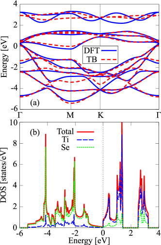
Figure 3: (a) Tight-binding (TB) bands of the monolayer TiSe₂ compared with the density-functional-theory (DFT) based bands used as the reference bands in the fitting of the TB parameters. The Fermi energy of the TB bands is set to zero, and thus the Fermi energy of the DFT bands is located at $-0.19$ eV. (b) Density of states (DOS) of the TB bands of the monolayer TiSe₂. The partial densities of states of the Ti (dashed line) and Se (dotted line) orbitals are also shown.

Table 1: Slater-Koster transfer integrals determined by fitting to the first-principles DFT bands shown in Fig. 3(a). In this fitting, the energy levels of the Ti $d\gamma$ ($d_{x^{2}-y^{2}}$, $d_{3z^{2}-r^{2}}$), Ti $d\varepsilon$ ($d_{xy}$, $d_{yz}$, $d_{zx}$), and Se $p$ ($p_{x}$, $p_{y}$, $p_{z}$) orbitals satisfy $\varepsilon_{d\gamma}-\varepsilon_{d\varepsilon}=1.112$ eV and $\varepsilon_{d\varepsilon}-\varepsilon_{p}=2.171$ eV. Note that $t(pd\sigma)=-t(dp\sigma)$ and $t(pd\pi)=-t(dp\pi)$.

Transfer Integral [eV]
$t(pd\sigma)$	=	$-$1.422		$t(pp\sigma)_{1}$	=	0.709
$t(pd\pi)$	=	0.797		$t(pp\pi)_{1}$	=	$-$0.103
$t(dd\sigma)$	=	$-$0.347		$t(pp\sigma)_{2}$	=	0.592
$t(dd\pi)$	=	0.119		$t(pp\pi)_{2}$	=	$-$0.009
$t(dd\delta)$	=	$-$0.030

Since a TiSe₆ has octahedral structure, we consider the energy levels $\varepsilon_{d\gamma}$, $\varepsilon_{d\varepsilon}$, and $\varepsilon_{p}$ of the Ti $d\gamma$ ($d_{x^{2}-y^{2}}$, $d_{3z^{2}-r^{2}}$), Ti $d\varepsilon$ ($d_{xy}$, $d_{yz}$, $d_{zx}$), and Se $p$ ($p_{x}$, $p_{y}$, $p_{z}$) orbitals, respectively Yoshida and Motizuki (1980); Suzuki et al. (1985); Motizuki (1986); Monney et al. (2011). The transfer integrals $t_{\mu\ell,\nu m}(\bm{R}_{n})$ are obtained by the Slater-Koster scheme Slater and Koster (1954) as the nine transfer integrals, $t(pd\sigma)$, $t(pd\pi)$, $t(dd\sigma)$, $t(dd\pi)$, $t(dd\delta)$, $t(pp\sigma)_{1}$, $t(pp\pi)_{1}$, $t(pp\sigma)_{2}$, and $t(pp\pi)_{2}$, where $t(pd\sigma)$ and $t(pd\pi)$ are the transfer integrals between the nearest-neighbor (NN) Ti 3$d$ and Se 4$p$ orbitals, and $t(dd\sigma)$, $t(dd\pi)$, and $t(dd\delta)$ are the transfer integrals between the NN Ti-Ti 3$d$ orbitals. The subscripts 1 and 2 in $t(pp\sigma)$ and $t(pp\pi)$ indicate the transfer integrals between the NN Se(1)-Se(1) [Se(2)-Se(2)] 4$p$ orbitals and between the NN Se(1)-Se(2) 4$p$ orbitals, respectively. The Slater-Koster transfer integrals are evaluated by a least-square fitting of the TB bands to the first-principles DFT bands along the high symmetry lines $\Gamma$-M-K-$\Gamma$. In the DFT band calculation , we use the full-potential linearized augmented-plane-wave method with the generalized gradient approximation (GGA) Perdew et al. (1996) for electron correlations implemented in the WIEN2k code Blaha et al. (2001). As the initial values of the parameters in the least-square fitting procedure, we use the Slater-Koster transfer integrals [$t(pd\sigma)$ etc.] roughly estimated from the TB bands obtained via the maximally localized Wannier functions Kuneš et al. (2010); Mostofi et al. (2008). We use 252 $\bm{k}$-points along the $\Gamma$-M-K-$\Gamma$ lines in our least-square fitting.

The optimized values of the transfer integrals are summarized in Table 1. The obtained TB bands are compared with the original DFT bands in Fig 3(a) to find a good agreement, indicating that our TB band structure can capture the overall character of the first-principles DFT band structure. We find that the valence bands are composed mainly of the Se $p$ ($p_{x}$, $p_{y}$, $p_{z}$) orbitals and the conduction bands near the Fermi level are composed mainly of the Ti $d\varepsilon$ ($d_{xy}$, $d_{yz}$, $d_{zx}$) orbitals. The Ti $d\gamma$ bands are located well above the $d\varepsilon$ bands due to the crystal field splitting $\varepsilon_{d\gamma}>\varepsilon_{d\varepsilon}$. The valence-band top is located at the $\Gamma$ point of the BZ and the conduction-band bottom is located at the M points of the BZ. The valence-band maximum and conduction-band minimum are +0.081 eV and -0.007 eV, respectively, from the Fermi level, resulting in the semimetallic band structure located in the vicinity of a zero-gap semiconducting state.

II.3 Electron-Phonon Coupling

To discuss the lattice displacements in TiSe₂, we introduce the electron-phonon coupling, following the method of Motizuki et al.. Yoshida and Motizuki (1980, 1980); Takaoka and Motizuki (1980); Motizuki et al. (1981a, b); Suzuki et al. (1984, 1985); Motizuki (1986). The electron-phonon coupling strengths are given by the changes in the transfer integrals with respect to the lattice displacements $\delta\bm{R}_{i\mu}$ from their equilibrium positions $\bm{R}_{i\mu}$. In the reciprocal lattice space, $\delta\bm{R}_{i\mu}$ is given by

$$\delta\bm{R}_{i\mu} =\frac{1}{\sqrt{N}}\sum_{\bm{q}}e^{i\bm{q}\cdot\bm{R}_{i}}\bm{u}_{\bm{q},\mu}$$

$$=\frac{1}{\sqrt{NM_{\mu}}}\sum_{\bm{q}}e^{i\bm{q}\cdot\bm{R}_{i}}\bm{\varepsilon}(\bm{q},\mu)Q_{\bm{q}},$$ (13)

where $\bm{u}_{\bm{q},{\mu}}$ is the lattice displacement in $\bm{q}$-space given by $\bm{u}_{\bm{q},\mu}=\left(\bm{\varepsilon}(\bm{q},\mu)/\sqrt{M_{\mu}}\right)Q_{\bm{q}}$. The displacement $\bm{u}_{\bm{q},\mu}$ is characterized by the normal coordinate $Q_{\bm{q}}$ and polarization vector $\bm{\varepsilon}(\bm{q},\mu)$ of a particular phonon mode at $\bm{q}$, where $M_{\mu}$ is the mass of atom $\mu$. Details of the derivation and general form of the electron-phonon coupling are summarized in Appendix A.1. In this approach, the Hamiltonian of the electron-phonon coupling is given by

$$\mathcal{H}_{ep}=\frac{1}{\sqrt{N}}\sum_{\bm{k},\bm{q}}\sum_{\mu\ell,\nu m}g_{\mu\ell,\nu m}(\bm{k},\bm{q})Q_{\bm{q}}c^{{\dagger}}_{\bm{k},\mu\ell}c_{\bm{k}-\bm{q},\nu m}$$ (14)

with the electron-phonon coupling constant

$$g_{\mu\ell,\nu m}(\bm{k},\bm{q}) =\sum_{\bm{R}_{n}}\left[\bm{\nabla}t_{\mu\ell,\nu m}(\bm{R}_{n})\right]$$ (15)

$$\cdot\left[\frac{\bm{\varepsilon}(\bm{q},\mu)}{\sqrt{M_{\mu}}}e^{-i(\bm{k}-\bm{q})\cdot\bm{R}_{n}}-\frac{\bm{\varepsilon}(\bm{q},\nu)}{\sqrt{M_{\nu}}}e^{-i\bm{k}\cdot\bm{R}_{n}}\right],$$

where $\bm{\nabla}t_{\mu\ell,\nu m}(\bm{R}_{n})$ is the first derivative of the transfer integral with respect to $\bm{R}_{n}$.

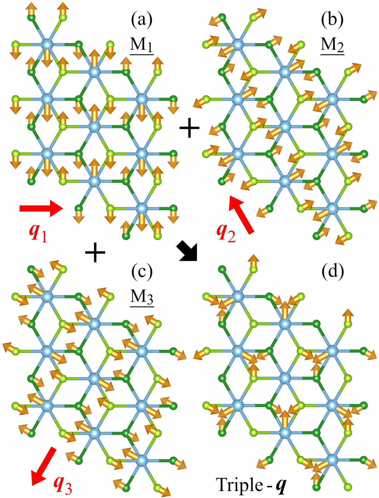
Figure 4: Schematic representation of the transverse phonon modes at the (a) M₁, (b) M₂ and (c) M₃ points of the BZ. (d) Periodic lattice displacement in the triple-$\bm{q}$ state.

In Fig. 4(d), we show the schematic picture of the periodic lattice displacement (PLD) observed experimentally in TiSe₂ Di Salvo et al. (1976). Realization of this PLD has been explained theoretically by Motizuki et al. Suzuki et al. (1985); Motizuki (1986). A first-principles calculation for this PLD has also been performed by Bianco $et$ $al$. Bianco et al. (2015). Accordingly, the 2$\times$2 PLD shown in Fig. 4(d) is realized by the sum of the transverse phonon modes at the M₁, M₂, and M₃ points of the BZ illustrated in Figs. 4(a)–4(c). Therefore the 2$\times$2 PLD is the triple-$\bm{q}$ structure characterized by the wave vectors $\bm{q}_{1}=\bm{b}_{1}/2$, $\bm{q}_{2}=(\bm{b}_{2}-\bm{b}_{1})/2$, and $\bm{q}_{3}=-\bm{b}_{2}/2$ shown in Fig. 2(b). In this paper, we consider the transverse phonon modes shown in Figs. 4(a)–4(c) as the specific phonon modes in Eqs. (13)–(15).

To estimate the coupling constants $g_{\mu\ell,\nu m}(\bm{k},\bm{q})$, we need the polarization vector $\bm{\varepsilon}(\bm{q},\mu)$ characterized by the eigenstate of the transverse phonon mode. $\bm{\varepsilon}(\bm{q},\mu)$ for the PLD in TiSe₂ has been provided by Motizuki et al. Suzuki et al. (1985); Motizuki (1986) (see also Appendix C). When the ratio between the lattice displacements of Ti and Se ions is given as $\xi=|\bm{u}_{\bm{q}_{j},{\rm Se}}|/|\bm{u}_{\bm{q}_{j},{\rm Ti}}|$, the polarization vectors for the transverse phonon mode at the M₁ point, which are perpendicular to the vector $\bm{q}_{1}$, are given by

$$\bm{\varepsilon}(\bm{q}_{1},{\rm Ti})=\sqrt{M_{\rm Ti}/M^{*}}\bm{e}_{Y},$$ (16)

$$\bm{\varepsilon}(\bm{q}_{1},{\rm Se1})=\bm{\varepsilon}(\bm{q}_{1},{\rm Se2})=-\xi\sqrt{M_{\rm Se}/M^{*}}\bm{e}_{Y},$$ (17)

where $M^{*}=M_{\rm Ti}+2\xi^{2}M_{\rm Se}$ is the effective mass of the transverse mode at the M point. Similarly, the polarization vectors $\bm{\varepsilon}(\bm{q}_{2},\mu)$ and $\bm{\varepsilon}(\bm{q}_{3},\mu)$ are perpendicular to their respective wave vectors (see also Appendix C). The ratio $\xi$ was estimated as $\xi\simeq 1/3$ in previous experimental Di Salvo et al. (1976); Fang et al. (2017) and theoretical Motizuki et al. (1981b); Bianco et al. (2015) studies. We therefore assume $\xi=1/3$ and $M^{*}=M_{\rm Ti}+(2/9)M_{\rm Se}$ ($=65.416$ u) Suzuki et al. (1985); Motizuki (1986) throughout this paper.

In addition to the polarization vector $\bm{\varepsilon}(\bm{q},\mu)$, the first derivative of the transfer integrals $\bm{\nabla}t_{\mu\ell,\nu m}(\bm{R}_{n})$ is required to estimate the coupling constants $g_{\mu\ell,\nu m}(\bm{k},\bm{q})$. Here we briefly describe the estimation of this quantity and the details are found in Appendix B. We follow the approximation introduced by Motizuki et al. Yoshida and Motizuki (1980); Motizuki (1986):

$$\frac{t^{\prime}(pd\sigma)}{t(pd\sigma)}=\alpha_{\rm c}\frac{s^{\prime}(pd\sigma)}{s(pd\sigma)},\;\;{\rm etc.},$$ (18)

where $t^{\prime}(pd\sigma)$ is the first derivative of the transfer integral $t(pd\sigma)$ with respect to the interatomic distance, and $s(pd\sigma)$ and $s^{\prime}(pd\sigma)$ indicate the overlap integral and its derivative, respectively. $\alpha_{\rm c}$ is the coupling constant that determines the strength of the electron-phonon coupling. In this paper, we treat $\alpha_{\rm c}$ as a tunable parameter; the value of $\alpha_{\rm c}$ is determined such that the calculated results are in good agreement with experiment. Note that $\alpha_{\rm c}=0$ does not indicate $g_{\mu\ell,\nu m}(\bm{k},\bm{q})=0$ since $\bm{\nabla}t_{\mu\ell,\nu m}(\bm{R}_{n})$ also includes the terms given by the transfer integrals $t(pd\sigma)$ (see Appendix B). In the estimation of the overlap integrals and their derivatives, we use the Slater-type orbital Slater (1930); Clementi and Raimondi (1963); Clementi et al. (1967). We can thus calculate the values analytically (see Appendix B). The Slater-type orbital is characterized by the orbital exponents, which are estimated by Clementi et al. Clementi and Raimondi (1963); Clementi et al. (1967): $\zeta_{3d}=2.7138$ and $\zeta_{4p}=2.0718$ for the Ti 3$d$ and Se 4$p$ orbitals, respectively. As shown in Fig. 3(b), the valence and conduction bands near the Fermi level are composed of Se $p$ ($p_{x}$, $p_{y}$, $p_{z}$) and Ti $d\varepsilon$ ($d_{xy}$, $d_{yz}$, $d_{zx}$) orbitals, respectively (see also Fig. 5). We therefore consider the electron-lattice coupling between the nearest-neighbor Ti $d\varepsilon$ ($d_{xy}$, $d_{yz}$, $d_{zx}$) and Se $p$ ($p_{x}$, $p_{y}$, $p_{z}$) orbitals only. In this approximation, we need the ratio between the overlap integral and its first derivative for both $pd\sigma$ and $pd\pi$; the estimated values given by the Slater-type orbitals are listed in Table 2.

Table 2: Ratio between the Slater-Koster overlap integral and its first derivative estimated by the Slater-type orbital. $s(pd\sigma)$ and $s(pd\pi)$ are the overlap integrals between nearest-neighbor Ti $d$ and Se $p$ orbitals. $s^{\prime}(pd\sigma)$ and $s^{\prime}(pd\pi)$ are the first derivative of the overlap integrals. In the Slater-type orbitals, we use the orbital exponents $\zeta_{3d}=2.7138$ and $\zeta_{4p}=2.0718$, for the Ti 3$d$ and Se 4$p$ orbitals, respectively Clementi and Raimondi (1963); Clementi et al. (1967). $R$ is the distance between Ti and Se ions: $R_{\rm Ti-Se}=2.566$ Å.

$R\times s^{\prime}(pd)/s(pd)$				$s^{\prime}(pd)/s(pd)$ [1/Å]
$R\!\times\!s^{\prime}(pd\sigma)/s(pd\sigma)$	​=​	$\!-$3.860		$s^{\prime}(pd\sigma)/s(pd\sigma)$	​=​	$\!-$1.504
$R\!\times\!s^{\prime}(pd\pi)/s(pd\pi)$	​=​	$\!-$5.933		$s^{\prime}(pd\pi)/s(pd\pi)$	​=​	$\!-$2.312

When the ions are displaced from their equilibrium position, the lattice system increases the elastic energy. The Hamiltonian of the elastic term is given by

$$\mathcal{H}_{p}=\frac{1}{2}\sum_{\bm{q}}\omega_{0}^{2}(\bm{q})|Q_{\bm{q}}|^{2},$$ (19)

where $\omega_{0}(\bm{q})$ is the bare phonon frequency of the transverse mode at momentum $\bm{q}$. A bare phonon frequency $\omega_{0}(\bm{q})$ has been estimated by Motizuki et al. in comparison with the experimentally observed phonon dispersions Motizuki et al. (1981a); Suzuki et al. (1985); Motizuki (1986). Monney et al. have also assumed the value close to it Monney et al. (2011). In this paper, we use a similar value $M^{*}\omega^{2}_{0}(\bm{q}_{\rm M})=10$ eV/Ų [$\omega_{0}(\bm{q}_{\rm M})\simeq 6.11$ THz] at the M point ($\bm{q}=\bm{q}_{\rm M}$). We may also treat $\omega_{0}(\bm{q}_{\rm M})$ as a tunable parameter.

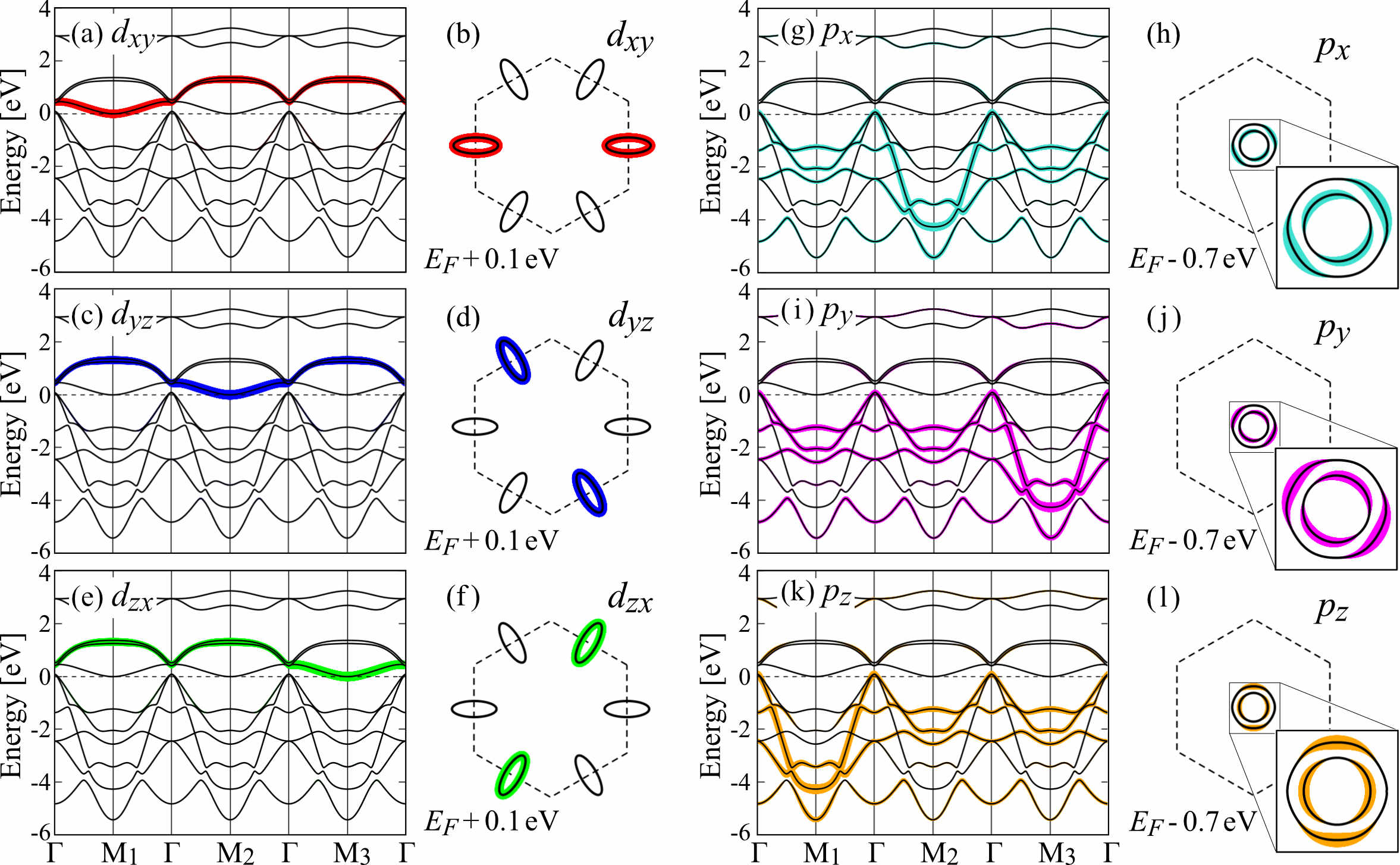
Figure 5: Weighted band dispersions and equal energy surfaces (lines) of the undistorted TB band structure. The width of the curves is in proportion to the weight of the (a, b) Ti $d_{xy}$, (c, d) Ti $d_{yz}$, (e, f) Ti $d_{zx}$, (g, h) Se $p_{x}$, (i, j) Se $p_{y}$, and (k, l) Se $p_{z}$ orbitals. In (b), (d), and (f), we plot the equal energy surfaces above the Fermi energy, $E_{F}+0.1$ eV, and in (h), (j), and (l), we plot the equal energy surfaces below the Fermi energy, $E_{F}-0.7$ eV. Dashed line indicates the original BZ without distortion.

II.4 Coulomb Interaction

To treat the excitonic mechanism of the CDW formation, we also consider the intersite Coulomb interactions. In general, the excitonic order (or excitonic insulator state) should be induced by the interband Coulomb interactions. In TiSe₂, the interband Coulomb (or excitonic) interactions are given by the interactions between the valence Se 4$p$ and the conduction Ti 3$d$ bands. In real space, the interband Coulomb (or excitonic) interaction in TiSe₂ is essentially given by the intersite Coulomb interaction between the nearest-neighbor Ti and Se sites. Therefore, as the excitonic interactions, we consider the intersite Coulomb interaction between the nearest-neighbor Ti and Se sites given by

$$\mathcal{H}_{ee}=\sum_{\bm{R}_{j},\bm{R}_{n}}\sum_{\ell,\nu m}V^{dp}_{\ell,\nu m}(\bm{R}_{n})n^{d}_{\ell}(\bm{R}_{j})n^{p}_{\nu m}(\bm{R}_{j}+\bm{R}_{n})$$

$$=\!\frac{1}{N}\!\sum_{\bm{k},\bm{k}^{\prime},\bm{q}}\sum_{\ell,\nu m}V^{dp}_{\ell,\nu m}(\bm{k}-\bm{k}^{\prime})d^{{\dagger}}_{\bm{k},\ell}d_{\bm{k}^{\prime},\ell}p^{{\dagger}}_{\bm{k}^{\prime}-\bm{q},\nu m}p_{\bm{k}-\bm{q},\nu m},$$ (20)

where $V^{dp}_{\ell,\nu m}(\bm{R}_{n})$ is the intersite Coulomb interaction between the nearest-neighbor Ti $d_{\ell}$ and Se($\nu$) $p_{m}$ orbitals, and $n^{d}_{\ell}(\bm{R}_{j})$ and $n^{p}_{\nu m}(\bm{R}_{j})$ are the number operators of the electron of the Ti $d_{\ell}$ and Se($\nu$) $p_{m}$ orbitals, respectively, in the unit cell at $\bm{R}_{j}$. Second line of Eq. (20) indicates the Fourier transformed Coulomb interaction, where

$$V^{dp}_{\ell,\nu m}(\bm{k}-\bm{k}^{\prime})=\sum_{\bm{R}_{n}}V^{dp}_{\ell,\nu m}(\bm{R}_{n})e^{-i(\bm{k}-\bm{k}^{\prime})\cdot\bm{R}_{n}},$$ (21)

and $d^{({\dagger})}_{\bm{k},\ell}$ and $p^{({\dagger})}_{\bm{k},\nu m}$ are the annihilation (creation) operators of an electron in the Ti $d_{\ell}$ and Se($\nu$) $p_{m}$ orbitals, respectively, at momentum $\bm{k}$. In this paper, we assume the orbital independent interaction, $V^{dp}_{\ell,\nu m}(\bm{R}_{n})=V$, for simplicity, and we treat $V$ as a tunable parameter.

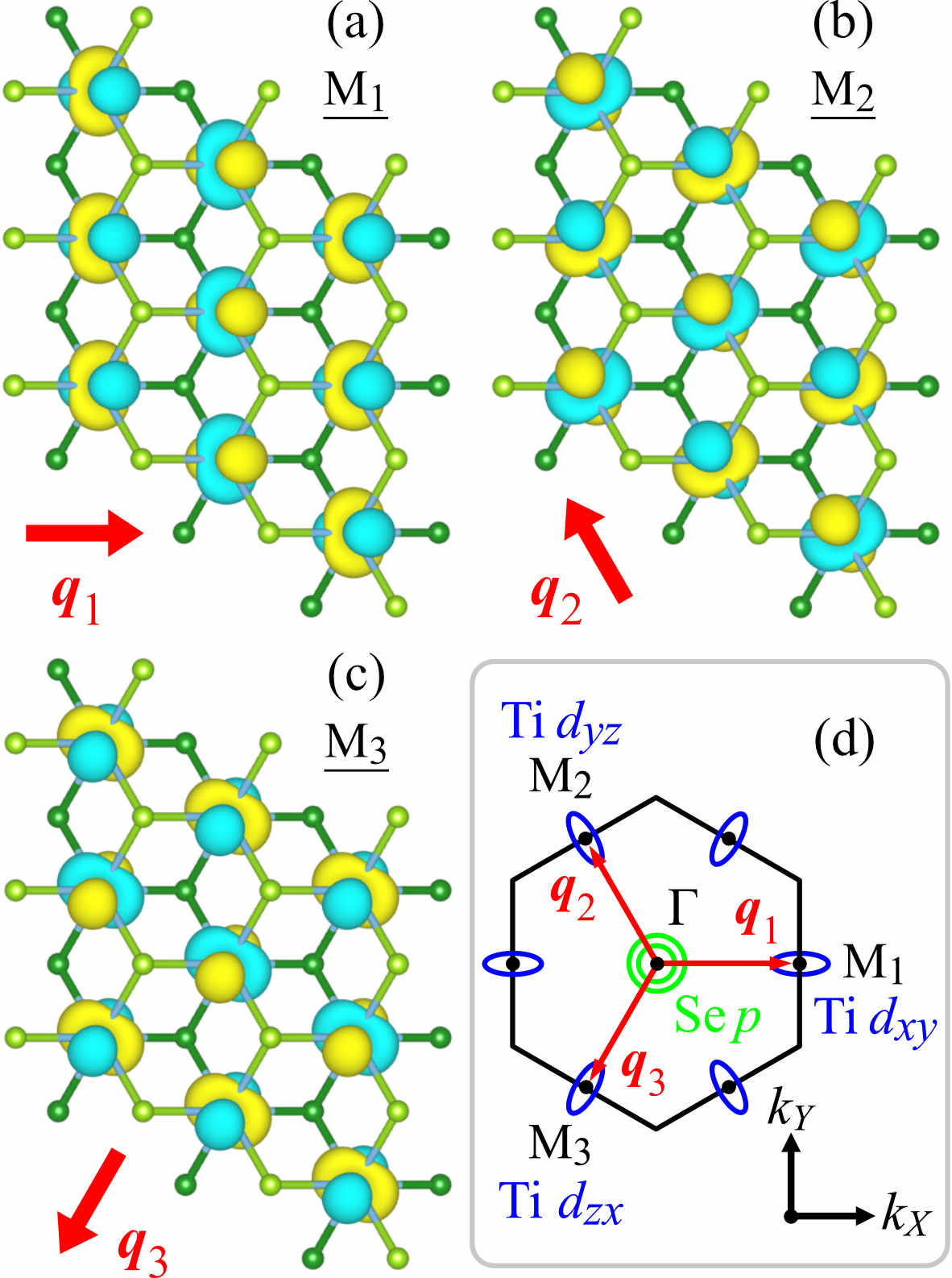
Figure 6: Bloch wave functions $\psi^{(0)}_{\bm{k},a}(\bm{r})$ of the conduction-band bottom at the (a) M₁, (b) M₂, and (c) M₃ points, where the Slater-type orbitals are employed as the atomic orbitals. (d) Schematic Fermi surfaces of the monolayer TiSe₂. Note that areas of the hole and electron pockets are slightly larger than those of our TB bands.

III Undistorted Band Structure

Before discussing the CDW state caused by the electron-phonon and excitonic interactions, we overview the characters of undistorted band structure given by diagonalizing the TB Hamiltonian $\mathcal{H}_{e}$.

Figure 5 shows the calculated band dispersions along the $\bm{k}$-path through the M₁, M₂, and M₃ points of the BZ defined in Fig. 2(b). Here, we also plot the weight of orbitals on each band given by $|u^{(0)}_{\mu\ell,a}(\bm{k})|^{2}$, where $u^{(0)}_{\mu\ell,a}(\bm{k})$ is the $\mu\ell$ component of the eigenvector for the band $a$. Figures 5(a), 5(c), and 5(e) show the weighted band dispersions of the Ti $d_{xy}$, $d_{yz}$, and $d_{zx}$ orbitals, respectively. We find that the Ti $d_{xy}$, $d_{yz}$, and $d_{zx}$ orbital characters appear in the conduction-band bottom at the M₁, M₂, and M₃ points of the BZ, respectively. To show the corresponding characters in $\bm{k}$-space, we also plot in Figs. 5(b),  5(d), and  5(f) the equal energy surfaces (lines) above the Fermi level $E_{F}$ with the weight of the Ti $d$ orbitals. We find that the equal energy surface around the M₁ point is almost completely composed of the Ti $d_{xy}$ orbital. Similarly, the equal energy surfaces around the M₂ and M₃ points are given by $d_{yz}$ and $d_{zx}$ orbitals, respectively. Thus the characters of the Ti $d_{xy}$, $d_{yz}$, and $d_{zx}$ orbitals are related to each other by the $2\pi/3$ rotation around the $\Gamma$ point. These results are consistent with the orbital characters in the bulk TiSe₂, which was pointed out by van Wezel van Wezel (2011). Figures 5(g)–5(l) show the weighted band dispersions and the equal energy surfaces below $E_{F}$ for the Se $p_{x}$, $p_{y}$, and $p_{z}$ orbitals. We find that the two valence bands around the $\Gamma$ point are composed of the Se $p$ orbitals but that the inequivalence in the weight of the $p_{x}$, $p_{y}$, and $p_{z}$ orbitals appears along the different $\bm{k}$-directions. The equal energy surfaces in the valence bands show the similar $2\pi/3$ rotational property of Se $p_{x}$, $p_{y}$, and $p_{z}$ orbitals around the $\Gamma$ point.

Figures 6(a)–6(c) show the Bloch wave functions $\psi^{(0)}_{\bm{k},a}(\bm{r})$ of the conduction-band bottoms at the M₁, M₂, and M₃ points. When the Hamiltonian in the TB approximation is diagonalized, the Bloch wave function of band $a$ is given by $\psi^{(0)}_{\bm{k},a}(\bm{r})=\sum_{\mu\ell}u^{(0)*}_{\mu\ell,a}(\bm{k})\phi^{(0)}_{\bm{k},\mu\ell}(\bm{r})$, where $\phi^{(0)}_{\bm{k},\mu\ell}(\bm{r})$ is the Bloch sum of the atomic orbitals $\phi^{(0)}_{\bm{k},\mu\ell}(\bm{r})=(1/\sqrt{N})\sum_{\bm{R}_{i}}\phi_{\ell}(\bm{r}-\bm{R}_{i\mu})e^{i\bm{k}\cdot\bm{R}_{i}}$ and we use the Slater-type orbital as the atomic orbital $\phi_{\ell}(\bm{r})$, as in the estimation of the overlap integrals discussed in Sec. II.3. We find in Fig. 6(a) that the Bloch wave function $\psi^{(0)}_{\bm{k},a}(\bm{r})$ at the M₁ point clearly shows the shape nearly consistent with the $d_{xy}$ orbital around Ti atoms. Note that, due to $e^{i\bm{k}\cdot\bm{R}_{i}}=e^{i\bm{q}_{1}\cdot\bm{R}_{i}}$ in the Bloch function at the M₁ point, the wave functions on Ti atoms change signs along the direction of $\bm{q}_{1}$. Similarly, the shapes of the $d_{yz}$ and $d_{zx}$ orbitals appear in the Bloch functions at the M₂ and M₃ points, respectively. Ti $d_{xy}$, $d_{yz}$, and $d_{zx}$ orbitals, which appear in the Bloch functions at the M₁, M₂, and M₃ points, respectively, are rotated by $2\pi/3$ around the $Z$ axis in the global coordinates due to the three-fold rotational symmetry of the crystal structure. We do not show the Bloch functions of the valence-band top at the $\Gamma$ point here, but we have confirmed that they clearly show the shapes of the $p$ orbitals around Se atoms.

Figure 6(d) summarizes the Fermi surfaces of the undistorted band structure of the monolayer TiSe₂ schematically. The hole pockets (i.e., valence-band top) at the $\Gamma$ point are characterized by the Se $p$ orbitals and the electron pockets (i.e., conduction-band bottom) at the M₁, M₂, and M₃ points are characterized by the Ti $d_{xy}$, $d_{yz}$, and $d_{zx}$ orbitals, respectively. The CDW state in TiSe₂ may therefore be given by the mixture of the Se $p$ orbitals at the $\Gamma$ point and Ti $d_{xy}$, $d_{yz}$, $d_{zx}$ orbitals at the M₁, M₂, and M₃ points.

IV Phonon Softening and CDW

In this section, we discuss the realization of the CDW without introducing the excitonic interaction. We first discuss the softening of the transverse modes at the M points shown in Figs. 4(a)–4(c). We then examine the stability of the static triple-$\bm{q}$ CDW state, where the transverse phonon modes at the M₁, M₂, and M₃ points are frozen simultaneously, as shown in Fig. 4(d).

IV.1 Phonon Softening

To discuss the structural instability in TiSe₂, we evaluate the effective phonon frequency $\omega(\bm{q})$ given as Motizuki (1986)

$$\omega^{2}(\bm{q})=\omega^{2}_{0}(\bm{q})-\chi(\bm{q}),$$ (22)

where $\omega_{0}(\bm{q})$ is the bare phonon frequency of the transverse mode and $\chi(\bm{q})$ is the susceptibility including the electron-phonon coupling $g_{\mu\ell,\nu m}(\bm{k},\bm{q})$ (see Appendix A.2). Specifically, the susceptibility $\chi(\bm{q})$ is given by

$$\chi(\bm{q})=\!-\frac{2}{N}\sum_{\bm{k}}\sum_{a,b}\left|V_{ep}(a\bm{k},b\bm{k}\!-\!\bm{q})\right|^{2}\!\frac{f(\varepsilon^{(0)}_{\bm{k},a})\!-\!f(\varepsilon^{(0)}_{\bm{k}-\bm{q},b})}{\varepsilon^{(0)}_{\bm{k},a}\!-\!\varepsilon^{(0)}_{\bm{k}-\bm{q},b}}$$ (23)

with

$$V_{ep}(a\bm{k},b\bm{k}\!-\!\bm{q})=\!\sum_{\mu\ell,\nu m}u^{(0)*}_{\mu\ell,a}(\bm{k})g_{\mu\ell,\nu m}(\bm{k},\bm{q})u^{(0)}_{\nu m,b}(\bm{k}\!-\!\bm{q}),$$ (24)

where $\varepsilon^{(0)}_{\bm{k},a}$ is the undistorted energy band, $u^{(0)}_{\mu\ell,a}(\bm{k})$ is the $\mu\ell$ component of the eigenvector for the band $a$, and $f(\varepsilon^{(0)}_{\bm{k},a})$ is the Fermi distribution function (see Appendix A.2). In the calculations of the susceptibility, we use $500\times 500$ $\bm{k}$ points for summation. In Eq. (18), we assume $\alpha_{\rm c}=0.1$, which provides results in good agreement with the observed lattice displacement Di Salvo et al. (1976) (see next subsection) if we use $M^{*}\omega^{2}_{0}(\bm{q}_{\rm M})=10$ eV/Ų as the bare phonon frequency $\omega_{0}(\bm{q})$ at the M point. In this section, we assume $\alpha_{\rm c}=0.1$ unless otherwise stated. The $\alpha_{\rm c}$ dependence will be discussed in the next section.

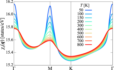
Figure 7: Calculated temperature dependence of the bare electronic susceptibility $\chi_{0}(\bm{q})$ as a function of $\bm{q}$.

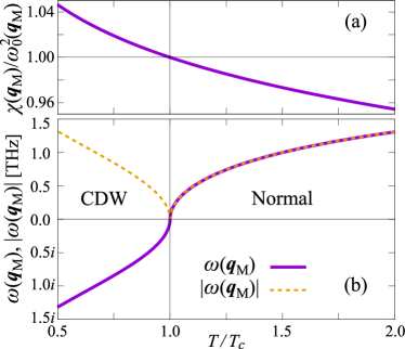
Figure 8: Calculated temperature dependence of the (a) susceptibility $\chi(\bm{q}_{\rm M})$ [$\chi(\bm{q}_{\rm M})/\omega^{2}_{0}(\bm{q}_{\rm M})$] and (b) effective phonon frequency $\omega(\bm{q}_{\rm M})$ at the M point. We assume $M^{*}\omega^{2}_{0}(\bm{q}_{\rm M})=10$ eV/Ų [$\omega_{0}(\bm{q}_{\rm M})\simeq 6.11$ THz], which gives the transition temperature $T_{c}\simeq 443$ K.

Before discussing the phonon softening, we show the character of the bare electronic susceptibility Yoshida and Motizuki (1980); Motizuki (1986); Calandra and Mauri (2011) given as

$$\chi_{0}(\bm{q})=-\frac{1}{N}\sum_{\bm{k}}\sum_{a,b}\frac{f(\varepsilon^{(0)}_{\bm{k},a})-f(\varepsilon^{(0)}_{\bm{k}-\bm{q},b})}{\varepsilon^{(0)}_{\bm{k},a}-\varepsilon^{(0)}_{\bm{k}-\bm{q},b}}.$$ (25)

Note that, if $\bm{k}$- and $\bm{q}$-dependences of $V_{ep}(a\bm{k},b\bm{k}\!-\!\bm{q})$ in Eq. (23) are negligible, $\chi_{0}(\bm{q})$ corresponds to $\chi(\bm{q})$. In Fig. 7, we show the calculated bare electronic susceptibility $\chi_{0}(\bm{q})$ at different temperatures $T$. The behavior of the $\bm{q}$ dependence of $\chi_{0}(\bm{q})$ reflects the band structure near $E_{F}$ [see Fig. 3(a)], which is in good agreement with previous theoretical estimates Yoshida and Motizuki (1980); Calandra and Mauri (2011). We find the temperature sensitive peak in $\chi_{0}(\bm{q})$ at the M point ($\bm{q}=\bm{q}_{\rm M}$), which corresponds to the wave vector of the CDW in monolayer TiSe₂. An enhancement of $\chi_{0}(\bm{q}_{\rm M})$ with decreasing temperature induces softening of the phonon mode at the M point. We note that $\chi_{0}(\bm{q})$ has a peak also at the $\Gamma$ point. However, previous studies have found that the phonon mode at the $\Gamma$ point does not show softening Motizuki et al. (1981a); Calandra and Mauri (2011); Bianco et al. (2015); Duong et al. (2015); Fu et al. (2016); Singh et al. (2017); Hellgren et al. (2017) because the phonon frequencies of the optical modes at the $\Gamma$ point is higher than the frequency of the softened transverse mode at the M point. We therefore consider the susceptibility $\chi(\bm{q})$ only at the M point in the following discussion.

Figure 8 shows the temperature dependence of the susceptibility $\chi(\bm{q})$ and effective phonon frequency $\omega(\bm{q})$ at the M point ($\bm{q}=\bm{q}_{\rm M}$), where we assume $M^{*}\omega^{2}_{0}(\bm{q}_{\rm M})=10$ eV/Ų [$\omega_{0}(\bm{q}_{\rm M})\simeq 6.11$ THz] as a bare phonon frequency. At this frequency $\omega_{0}(\bm{q}_{\rm M})$, we find that the susceptibility $\chi(\bm{q}_{\rm M})$ becomes larger than $\omega^{2}_{0}(\bm{q}_{\rm M})$ at $T\simeq 443$ K. To show this character clearly, we plot $\chi(\bm{q}_{\rm M})/\omega^{2}_{0}(\bm{q}_{\rm M})$ as a function of $T$ in Fig. 8(a). When the susceptibility reaches $\chi(\bm{q}_{\rm M})/\omega^{2}_{0}(\bm{q}_{\rm M})=1$, the effective phonon frequency $\omega(\bm{q}_{\rm M})$ [$=\omega_{0}(\bm{q}_{\rm M})\sqrt{1-\chi(\bm{q}_{\rm M})/\omega_{0}^{2}(\bm{q}_{\rm M})}$] vanishes, resulting in the structural phase transition. The transition temperature $T_{c}$ is given by $\omega(\bm{q}_{\rm M})=0$, or $\chi(\bm{q}_{\rm M})/\omega^{2}_{0}(\bm{q}_{\rm M})=1$, in this estimation. Although $T_{c}$ is higher than the experimental value in this parameter setting, the temperature dependent curve of $\omega(\bm{q}_{\rm M})$ is in good agreement with experimental result obtained by the x-ray diffuse scattering Holt et al. (2001).

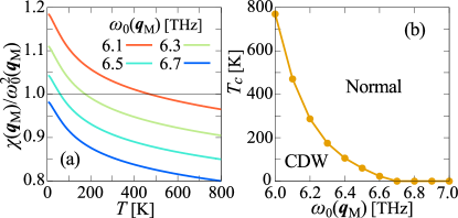
Figure 9: (a) Calculated temperature dependence of $\chi(\bm{q}_{\rm M})/\omega^{2}_{0}(\bm{q}_{\rm M})$ at different values of $\omega_{0}(\bm{q}_{\rm M})$. (b) Calculated transition temperature $T_{c}$ as a function of $\omega_{0}(\bm{q}_{\rm M})$.

To investigate $\omega_{0}(\bm{q}_{\rm M})$-dependence of the critical temperature $T_{c}$, we also show the temperature dependence of $\chi(\bm{q}_{\rm M})/\omega^{2}_{0}(\bm{q}_{\rm M})$ in Fig. 9(a) for different values of $\omega_{0}(\bm{q}_{\rm M})$. With increasing $\omega_{0}(\bm{q}_{\rm M})$ and thus decreasing $\chi(\bm{q}_{\rm M})/\omega^{2}_{0}(\bm{q}_{\rm M})$, $T_{c}$ is suppressed and vanishes at $\omega_{0}(\bm{q}_{\rm M})=6.7$ THz. Figure 9(b) shows the transition temperature $T_{c}$ as a function of $\omega_{0}(\bm{q}_{\rm M})$. We find that the calculated $T_{c}$ is in good agreement with the experimental value $T_{c}\simeq 200$ K when $\omega_{0}(\bm{q}_{\rm M})=6.2-6.3$ THz. Note that the estimation of $\chi({\bm{q}})$ in Eq. (23) corresponds to a random phase approximation Motizuki (1986) and overestimations of $T_{c}$ may be due to this approximation.

IV.2 Triple-$\bm{q}$ CDW

In this subsection, we discuss the stability of the static triple-$\bm{q}$ CDW state induced by the electron-phonon coupling $g_{\mu\ell,\nu m}(\bm{k},\bm{q})$. Here, we estimate the change in the total energy when the static triple-$\bm{q}$ crystal structure shown in Fig. 4(d) is realized.

When the transverse phonon modes at $\bm{q}_{1}$, $\bm{q}_{2}$, and $\bm{q}_{3}$ are frozen simultaneously, the corresponding expectation value is $\braket{Q_{\bm{q}_{j}}}=\sqrt{NM^{*}}u$ and the electron-phonon coupling in the static triple-$\bm{q}$ structure is given by

$$\mathcal{H}_{ep}=\sum_{\bm{k},\bm{q}_{j}}\sum_{\mu\ell,\nu m}\bar{g}_{\mu\ell,\nu m}(\bm{k},\bm{q}_{j})uc^{{\dagger}}_{\bm{k},\mu\ell}c_{\bm{k}-\bm{q}_{j},\nu m},$$ (26)

where $\bar{g}_{\mu\ell,\nu m}(\bm{k},\bm{q}_{j})\equiv\sqrt{M^{*}}g_{\mu\ell,\nu m}(\bm{k},\bm{q}_{j})$ for $\bm{q}_{j}=\bm{q}_{1}$, $\bm{q}_{2}$, $\bm{q}_{3}$ and $u$ corresponds to the magnitude of the displacement of the Ti atoms Suzuki et al. (1985); Motizuki (1986). Since Eq. (26) is not diagonal for $\bm{k}$ in the original BZ without distortion, we must introduce the reduced BZ (RBZ) shown in Fig. 2(b). In order to write the Hamiltonian simply in the matrix notation, here we introduce the 11$\times$11 matrices of the transfer integral $\hat{t}(\bm{k})$ and electron-phonon coupling $\hat{\bar{g}}(\bm{k},\bm{q})$, and the eleven dimensional vector of the annihilation (creation) operator $\bm{c}^{({\dagger})}_{\bm{k}}$. When we define the row vector $\bar{\bm{c}}^{{\dagger}}_{\bm{k}}=(\,\bm{c}^{{\dagger}}_{\bm{k}_{0}}\;\bm{c}^{{\dagger}}_{\bm{k}_{1}}\;\bm{c}^{{\dagger}}_{\bm{k}_{2}}\;\bm{c}^{{\dagger}}_{\bm{k}_{3}}\,)$ with $\bm{k}_{j}=\bm{k}-\bm{q}_{j}$ and $\bm{q}_{0}=\bm{0}$, the Hamiltonian of the tight-binding band and electron-phonon coupling $\mathcal{H}_{cdw}^{ep}=\mathcal{H}_{e}+\mathcal{H}_{ep}$ may be written as

$$\mathcal{H}_{cdw}^{ep}=\sum_{\bm{k}\in{\rm RBZ}}\bar{\bm{c}}^{{\dagger}}_{\bm{k}}\hat{\mathcal{H}}^{ep}_{\bm{k}}\bar{\bm{c}}_{\bm{k}}=\sum_{\bm{k}\in{\rm RBZ}}\sum_{i,j}\bm{c}^{{\dagger}}_{\bm{k}_{i}}\hat{\mathcal{H}}^{ep}_{\bm{k}_{i},\bm{k}_{j}}\bm{c}_{\bm{k}_{j}},$$ (27)

where $\hat{\mathcal{H}}^{ep}_{\bm{k}_{i},\bm{k}_{j}}$ is the 11$\times$11 block matrix of $(\bm{k}_{i},\bm{k}_{j})$ component of $\hat{\mathcal{H}}^{ep}_{\bm{k}}$ and is given as

$$\hat{\mathcal{H}}^{ep}_{\bm{k}_{i},\bm{k}_{j}}=\begin{cases}\hat{t}({\bm{k}_{i}})&(\bm{k}_{i}=\bm{k}_{j})\\ \hat{\bar{g}}(\bm{k}_{i},\bm{q}_{i}+\bm{q}_{j})u&(\bm{k}_{i}\neq\bm{k}_{j})\end{cases}.$$ (28)

We estimate the distorted energy band $\varepsilon_{\bm{k},a}$ in the static triple-$\bm{q}$ structure by diagonalizing the 44$\times$44 matrix $\hat{\mathcal{H}}^{ep}_{\bm{k}}$ in the RBZ. See Appendix C for details.

Figure 10(a) shows the calculated energy bands $\varepsilon_{\bm{k},a}$ of the undistorted ($u/a=0$) and triple-$\bm{q}$ superlattice ($u/a=0.02$) structures in the RBZ. In the normal state, the conduction-band bottoms at the M points are folded to the $\Gamma$ point of the RBZ and the semi-metallic state is realized with the small band overlap. When the electron-phonon coupling induces the lattice displacement with $u\neq 0$, the band hybridization occurs to open the band gap around the $\Gamma$ point in the RBZ.

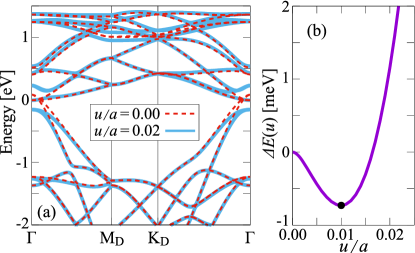
Figure 10: (a) Calculated band dispersions of TiSe₂ in the undistorted structure ($u/a=0$) and triple-$\bm{q}$ superlattice structure ($u/a=0.02$) displayed in the RBZ. The energy 0 corresponds to the Fermi energy in the undistorted structure ($u/a=0$). (b) Calculated energy $\Delta E(u)$ as a function of $u$. We assume $\alpha_{\rm c}=0.1$ and $M^{*}\omega^{2}_{0}(\bm{q}_{\rm M})=10$ eV/Ų [$\omega_{0}(\bm{q}_{\rm M})\simeq 6.11$ THz], and $a$ ($=3.54$ Å) is the lattice constant. A solid dot indicates the stationary point in (b).

By the gap opening at the Fermi level, the electronic energy in the triple-$\bm{q}$ structure is lowered. The energy difference at zero temperature is simply given as

$$\Delta E_{\rm elec}(u)=\frac{2}{N}\left[\sum_{\bm{k},a}^{{\rm occ.}}\varepsilon_{\bm{k},a}(u)-\sum_{\bm{k},a}^{{\rm occ.}}\varepsilon_{\bm{k},a}(0)\right],$$ (29)

where $\varepsilon_{\bm{k},a}(u)$ and $\varepsilon_{\bm{k},a}(0)$ are the band energies in the triple-$\bm{q}$ and undistorted structures, respectively, and ${\rm occ.}$ indicates the sum over the occupied $\bm{k}$ points in the RBZ. $N$ and 2 in Eq. (29) correspond to the number of the unit cells in the normal phase and spin degrees of freedom, respectively. When the atoms are displaced from their equilibrium positions, the energy of the lattice system increases as

$$\Delta E_{\rm elas}(u)=\frac{1}{2}\sum_{\bm{q}_{j}}M^{*}\omega^{2}_{0}(\bm{q}_{j})u^{2},$$ (30)

where $\omega_{0}(\bm{q}_{j})$ [$=\omega_{0}(\bm{q}_{\rm M})$] is the bare phonon frequency for $\bm{q}_{j}=\bm{q}_{1}$, $\bm{q}_{2}$, and $\bm{q}_{3}$. The sum of the electronic and elastic terms in Eqs. (29) and (30) gives the change in the total energy in the triple-$\bm{q}$ structure,

$$\Delta E(u)=\Delta E_{\rm elec}(u)+\Delta E_{\rm elas}(u).$$ (31)

Figure 10(b) shows the calculated $\Delta E(u)$ as a function of $u$, where we assume $M^{*}\omega^{2}_{0}(\bm{q}_{\rm M})\!=\!10$ eV/Ų [$\omega_{0}(\bm{q}_{\rm M})\!\simeq\!6.11$ THz] and $\alpha_{\rm c}=0.1$ in the electron-phonon coupling $g_{\mu\ell,\nu m}(\bm{k},\bm{q}_{j})$. The sum over $\bm{k}$ in Eq. (29) is evaluated by the tetrahedron method Blöchl et al. (1994) with a sampling of 100$\times$100 $\bm{k}$ points in the RBZ. In this parameter setting, the energy curve of $\Delta E(u)$ has a stationary point at a finite value of $u$, indicating the realization of the stable triple-$\bm{q}$ CDW state. The calculated lattice displacement $u/a=0.010$ at the stationary point is consistent with the experimental value $u/a=0.012$ estimated by the neutron diffraction Di Salvo et al. (1976). Recent x-ray study for monolayer TiSe₂ also observed a consistent value Fang et al. (2017).

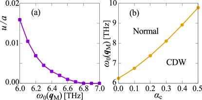
Figure 11: (a) Calculated lattice displacement $u$ in the triple-$\bm{q}$ CDW state as a function of $\omega_{0}(\bm{q}_{\rm M})$ at $\alpha_{\rm c}=0.1$. $a$ ($=3.54$ Å) is the lattice constant. (b) Calculated phase boundary between the normal ($u=0$) and triple-$\bm{q}$ CDW ($u\neq 0$) states.

We also check the stability of the triple-$\bm{q}$ CDW state for different values of $\omega_{0}(\bm{q}_{\rm M})$ and $\alpha_{\rm c}$ at $T=0$. In Fig. 11(a), we show the stationary $u$ point in $\Delta E(u)$ as a function of $\omega_{0}(\bm{q}_{\rm M})$ at $\alpha_{\rm c}=0.1$. The lattice displacement $u$ is suppressed with increasing $\omega_{0}(\bm{q}_{\rm M})$ and vanishes at $\omega_{0}(\bm{q}_{\rm M})=6.8$ THz. Note that the phase boundary of $\omega_{0}(\bm{q}_{\rm M})$ shown in Fig. 11(a) is slightly larger than the boundary shown in Fig. 9(b) estimated from the phonon softening $\chi(\bm{q}_{\rm M})/\omega^{2}_{0}(\bm{q}_{\rm M})$. This is because the susceptibility $\chi(\bm{q})$ is derived from the perturbation for a single-$\bm{q}$ phonon mode (see Appendix. A.2) and the triple-$\bm{q}$ CDW state including the couplings among different $\bm{q}$ phonon modes is more stable than a single-$\bm{q}$ CDW state, which is also discussed in Refs. Suzuki et al. (1985) and Bianco et al. (2015). As shown in Fig. 11(a), the lattice displacement $u$ is in good agreement with the experimental value when $\omega_{0}(\bm{q}_{\rm M})=6.0$ – $6.1$ THz. Moreover, we estimate in Fig. 11(b) the phase boundary between the normal ($u=0$) and triple-$\bm{q}$ CDW ($u\neq 0$) state in the parameter space of $\alpha_{\rm c}$ and $\omega_{0}(\bm{q}_{\rm M})$ at $T=0$. We find that, with increasing $\alpha_{\rm c}$, the triple-$\bm{q}$ CDW state becomes more stable due to the enhancement of the electron-phonon coupling $g_{\mu\ell,\nu m}(\bm{k},\bm{q})$, despite the fact that the bare phonon frequency $\omega_{0}(\bm{q}_{\rm M})$ becomes larger.

V Roles of Excitonic Interaction

In this section, we treat the intersite Coulomb interaction term $\mathcal{H}_{ee}$ in the mean-field approximation and discuss roles of the excitonic interaction for the triple-$\bm{q}$ CDW state shown in the previous section. Hereafter, we assume $\alpha_{\rm c}=0.1$ in the electron-phonon coupling $g_{\mu\ell,\nu m}(\bm{k},\bm{q})$ unless otherwise indicated.

V.1 Excitonic Order

Let us briefly discuss the mean-field approximation for the intersite Coulomb interaction term $\mathcal{H}_{ee}$. Details of the calculations are given in Appendix D. In TiSe₂, the locations of the top of the valence Se $p$ bands and the bottom of the conduction Ti $d$ bands are separated in momentum space by $\bm{q}_{j}=\bm{q}_{1}$, $\bm{q}_{2}$, and $\bm{q}_{3}$. We therefore introduce the excitonic order parameters defined by

$$\Delta^{dp}_{\ell,\nu m}(\bm{k},\bm{q}_{j})\!\equiv\!-\frac{1}{N}\sum_{\bm{k}^{\prime}}V^{dp}_{\ell,\nu m}(\bm{k}\!-\!\bm{k}^{\prime})\braket{p^{{\dagger}}_{\bm{k}^{\prime}-\bm{q}_{j},\nu m}d_{\bm{k}^{\prime},\ell}},$$ (32)

for $\bm{q}_{j}=\bm{q}_{1}$, $\bm{q}_{2}$, $\bm{q}_{3}$. The order parameters thus defined indicate the spontaneous hybridization between the Se $p$ and Ti $d$ bands due to the Coulomb interaction $V^{dp}_{\ell,\nu m}(\bm{k}\!-\!\bm{k}^{\prime})$, which results in the excitonic CDW state. The driving force of the CDW state is hence the interband Coulomb interaction. The mean-field Hamiltonian may then be written as $\mathcal{H}_{ee}\sim\mathcal{H}^{\rm MF}_{ee}=\mathcal{H}^{ex}_{cdw}+E^{ex}_{0}$ with

$$\mathcal{H}^{ex}_{cdw} =\sum_{\bm{k},\bm{q}_{j}}\sum_{\ell,\nu m}\Delta^{dp}_{\ell,\nu m}(\bm{k},\bm{q}_{j})d^{{\dagger}}_{\bm{k},\ell}p_{\bm{k}-\bm{q}_{j},\nu m}+{\mathrm{H.c.}},$$ (33)

$$E^{ex}_{0} =-\sum_{\bm{k},\bm{q}_{j}}\sum_{\ell,\nu m}\Delta^{dp}_{\ell,\nu m}(\bm{k},\bm{q}_{j})\braket{d^{{\dagger}}_{\bm{k},\ell}p_{\bm{k}-\bm{q}_{j},\nu m}}.$$ (34)

We may write the Hamiltonian in the matrix form in the RBZ, using the 5$\times$6 matrix of the order parameter $\hat{\Delta}(\bm{k},\bm{q}_{j})$, the five-dimensional vector of the annihilation (creation) operator of Ti $d$ orbitals $\bm{d}^{({\dagger})}_{\bm{k}}$, and six-dimensional vector of the annihilation (creation) operator of Se($\nu$) $p$ orbitals $\bm{p}^{({\dagger})}_{\bm{k}}$. Thus we may rewrite Eq. (33) as

$$\mathcal{H}^{ex}_{cdw}=\!\sum_{\bm{k}\in{\rm RBZ}}\bar{\bm{c}}^{{\dagger}}_{\bm{k}}\hat{\mathcal{H}}^{ex}_{\bm{k}}\bar{\bm{c}}_{\bm{k}}=\!\sum_{\bm{k}\in{\rm RBZ}}\sum_{i\neq j}\bm{c}^{{\dagger}}_{\bm{k}_{i}}\hat{\mathcal{H}}^{ex}_{\bm{k}_{i},\bm{k}_{j}}\bm{c}_{\bm{k}_{j}},$$ (35)

where $\bm{c}^{{\dagger}}_{\bm{k}_{i}}=(\,\bm{d}^{{\dagger}}_{\bm{k}_{i}}\;\bm{p}^{{\dagger}}_{\bm{k}_{i}}\,)$ and $\hat{\mathcal{H}}^{ex}_{\bm{k}_{i},\bm{k}_{j}}$ is the 11$\times$11 block matrix consisting of the $(\bm{k}_{i},\bm{k}_{j})$ components of $\hat{\mathcal{H}}^{ex}_{\bm{k}}$, i.e.,

$$\hat{\mathcal{H}}^{ex}_{\bm{k}_{i},\bm{k}_{j}}=\left[\begin{array}[]{c c }\hat{0}&\hat{\Delta}(\bm{k}_{i},\bm{q}_{i}+\bm{q}_{j})\\ \hat{\Delta}^{{\dagger}}(\bm{k}_{j},\bm{q}_{i}+\bm{q}_{j})&\hat{0}\\ \end{array}\right].$$ (38)

In the calculation, we assume the excitonic order parameters defined between the nearest-neighbor Ti $d\varepsilon$ ($d_{xy}$, $d_{yz}$, $d_{zx}$) and Se $p$ ($p_{x}$, $p_{y}$, $p_{z}$) orbitals only. We diagonalize the mean-field Hamiltonian, $\hat{\mathcal{H}}^{ex}_{\bm{k}}$ defined above plus $\hat{\mathcal{H}}^{ep}_{\bm{k}}$ defined in Eq. (27), and optimize the order parameter $\hat{\Delta}(\bm{k}_{i},\bm{q}_{j})$ self-consistently at each value of the lattice displacement $u$. Using the band dispersion with the optimized order parameters, we evaluate $\Delta E(u)=\Delta E_{\rm elec}(u)+\Delta E_{\rm elas}(u)+E^{ex}_{0}/N$ and find the stationary point of $\Delta E(u)$. In the self-consistent calculation, we use a sampling of 50$\times$50 $\bm{k}$ points in the RBZ.

Figure 12: (a) Calculated energy $\Delta E(u)$ as a function of $u$ with different values of $V$. We assume $M^{*}\omega^{2}_{0}(\bm{q}_{\rm M})=10$ eV/Ų and $a=3.54$ Å. Solid dots indicate the stationary points. (b) Calculated lattice displacement $u$ at the stationary point and the corresponding order parameter $\bar{\Delta}(\bm{q}_{j})$ as a function of $V$.

V.2 Enhancement of CDW

Figure 12(a) shows the calculated $u$ dependence of the energy $\Delta E(u)$ at $M^{*}\omega^{2}_{0}(\bm{q}_{\rm M})=10$ eV/Ų for different values of the Coulomb interaction $V$ [$=V^{dp}_{\ell,\nu m}(\bm{R}_{n})$]. We find that, with increasing $V$, the energy of the triple-$\bm{q}$ CDW state becomes more stable and the lattice displacement $u$ at the stationary point is enhanced. The stationary values of $u$ are shown in Fig. 12(b) as a function of $V$, which clearly indicates that the excitonic (intersite Coulomb) interactions stabilize the triple-$\bm{q}$ CDW state in TiSe₂, working cooperatively with the electron-phonon coupling.

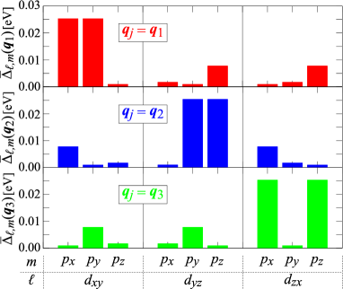
Figure 13: Orbital dependence of the averaged order parameters: $\bar{\Delta}_{\ell,m}(\bm{q}_{1})$ (upper panels), $\bar{\Delta}_{\ell,m}(\bm{q}_{2})$ (middle panels), and $\bar{\Delta}_{\ell,m}(\bm{q}_{3})$ (lower panels) at $V=0.3$ eV. Also see Fig. 12.

To study the character of the excitonic ordering, we calculate the average of the absolute values of the order parameters defined by

$$\bar{\Delta}_{\ell,m}(\bm{q}_{j})\equiv\frac{1}{N}\sum_{\bm{k}\in{\rm RBZ}}\sum_{i=0}^{3}\sum_{\nu=1,2}|\Delta^{dp}_{\ell,\nu m}(\bm{k}_{i},\bm{q}_{j})|.$$ (39)

As an indicator of the excitonic ordering, we also define the total value of the averaged order parameters $\bar{\Delta}_{\ell,m}(\bm{q}_{j})$,

$$\bar{\Delta}(\bm{q}_{j})\equiv\sum_{\ell,m}\bar{\Delta}_{\ell,m}(\bm{q}_{j}).$$ (40)

As shown in Fig. 12(b), the calculated total order parameter $\bar{\Delta}(\bm{q}_{j})$ satisfies the relation $\bar{\Delta}(\bm{q}_{1})=\bar{\Delta}(\bm{q}_{2})=\bar{\Delta}(\bm{q}_{3})$ due to the three-fold rotational symmetry. With increasing $V$, $\bar{\Delta}(\bm{q}_{j})$ increases monotonically from $\bar{\Delta}(\bm{q}_{j})=0$ at $V=0$, which indicates that the excitonic order coexists with the phononic triple-$\bm{q}$ CDW order and enhances the $d$-$p$ hybridizations, supporting the realization of the stable triple-$\bm{q}$ CDW state.

Figure 13 shows the orbital dependence of the averaged order parameters $\bar{\Delta}_{\ell,m}(\bm{q}_{j})$ at $V=0.3$ eV. We find that the components between the Ti $d_{xy}$ orbital and Se $p_{x}$ and $p_{y}$ orbitals [$\bar{\Delta}_{xy,x}(\bm{q}_{1})=\bar{\Delta}_{xy,y}(\bm{q}_{1})$] are dominant in the order parameter with $\bm{q}_{1}$. This behavior is understood from the orbital character of the undistorted band structure shown in Figs. 5 and  6; the conduction band around the M₁ point is mostly given by the Ti $d_{xy}$ orbital and the valence bands around the $\Gamma$ point are mostly given by the Se $p$ orbitals. We find that the components $\bar{\Delta}_{xy,x}(\bm{q}_{1})$ and $\bar{\Delta}_{xy,y}(\bm{q}_{1})$ are dominant but the component $\bar{\Delta}_{xy,z}(\bm{q}_{1})$ is very small. This is because the Se $p_{z}$ orbital are nearly perpendicular to the Ti $d_{xy}$ orbital but the Se $p_{x}$ and $p_{y}$ orbitals can enhance the $pd\pi$ bonding with the Ti $d_{xy}$ orbital. In the same way, the $d_{yz}$ components are dominant in the order parameter with $\bm{q}_{2}$ [$\bar{\Delta}_{yz,y}(\bm{q}_{2})=\bar{\Delta}_{yz,z}(\bm{q}_{2})$] and the $d_{zx}$ components are dominant in the order parameter with $\bm{q}_{3}$ [$\bar{\Delta}_{zx,z}(\bm{q}_{3})=\bar{\Delta}_{zx,x}(\bm{q}_{3})$], reflecting the orbital character in the undistorted band dispersions.

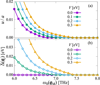
Figure 14: Calculated $\omega_{0}(\bm{q}_{\rm M})$ dependence of (a) the lattice displacement $u$ and (b) order parameter $\bar{\Delta}(\bm{q}_{j})$ for different values of $V$. $a$ $(=3.54$ Å) is the lattice constant.

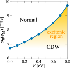
Figure 15: Calculated ground-state phase diagram of the triple-$\bm{q}$ CDW state in the parameter space of $V$ and $\omega_{0}(\bm{q}_{\rm M})$.

We also check the stability of the triple-$\bm{q}$ CDW state for different values of $\omega_{0}(\bm{q}_{\rm M})$ and $V$. Figure 14 shows $\omega_{0}(\bm{q}_{\rm M})$ dependence of the lattice displacement $u$ and order parameter $\bar{\Delta}(\bm{q}_{j})$ for different values of $V$. With increasing $\omega_{0}(\bm{q}_{\rm M})$, the PLD in the triple-$\bm{q}$ CDW state is suppressed, but with increasing $V$, the lattice displacement $u$ is enhanced. Similarly, $\bar{\Delta}(\bm{q}_{j})$ is suppressed with increasing $\omega_{0}(\bm{q}_{\rm M})$. We note that the pure excitonic state, where the triple-$\bm{q}$ CDW state occurs without lattice displacements, is not realized in our calculations, similar to the previous report in Refs. Zenker et al. (2013) and Watanabe et al. (2015). Figure 15 shows the ground-state phase diagram in the parameter space of $V$ and $\omega_{0}(\bm{q}_{\rm M})$. Apparently, the area of the triple-$\bm{q}$ CDW phase is enlarged with increasing $V$. The excitonic interaction $V$ thus enhances the triple-$\bm{q}$ CDW state in TiSe₂. We may therefore regard the CDW state in this enlarged region as the exciton-induced CDW state.

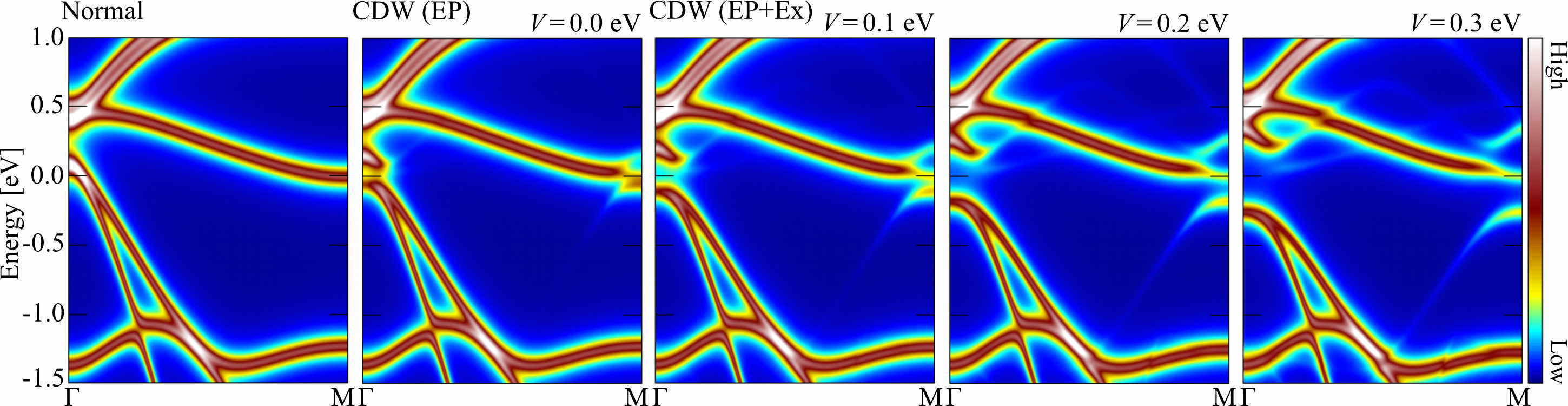
Figure 16: Calculated single-particle spectra $A(\bm{k},\omega)$ of the normal and triple-$\bm{q}$ CDW states of the monolayer TiSe₂, presented in the unfolded BZ. We assume the self-consistent solutions for $V=0.0$, $0.1$, $0.2$, and $0.3$ eV shown in Fig. 12. The spectra are broadened with $\eta=0.05$ eV. The energy zero is set to the lowest edge of the band above the Fermi level.

VI Electronic structure in CDW

In order to discuss the electronic structure of the triple-$\bm{q}$ CDW state, here we calculate the single-particle spectrum, simulating the angle-resolved photoemission spectroscopy (ARPES), and also the electronic charge density distribution in the TB approximation, discussing the local charge distribution in the CDW state of TiSe₂.

VI.1 Single-particle Spectrum

In our one-body approximation, the single-particle spectrum is given by

$$A(\bm{k},\omega)=\sum_{\mu\ell}\sum_{a}|u_{\bm{q}_{0}\mu\ell,a}(\bm{k})|^{2}\delta(\omega-\varepsilon_{\bm{k},a}),$$ (41)

where $u_{\bm{q}_{0}\mu\ell,a}(\bm{k})$ is the coefficient of the unitary transformation $c_{\bm{k}-\bm{q}_{j},\mu\ell}=\sum_{a}u_{\bm{q}_{j}\mu\ell,a}(\bm{k})\gamma_{\bm{k},a}$ in the diagonalization of the 44$\times$44 Hamiltonian matrix $\hat{\mathcal{H}}^{ep}_{\bm{k}}+\hat{\mathcal{H}}^{ex}_{\bm{k}}$. Detailed derivation is given in Appendix E. In the spectral calculation, each $\delta$-function in Eq. (41) is represented by a Lorentzian function with a finite broadening factor $\eta$.

Calculated results for $A(\bm{k},\omega)$ in the normal and triple-$\bm{q}$ CDW states are shown in Fig. 16 along the line $\Gamma-\mathrm{M}$ $(\mathrm{M}_{1}$) of the unfolded BZ. We assume $V=0.0$, $0.1$, $0.2$, and $0.3$ eV to obtain the self-consistent solutions for the CDW states as in Fig. 12. In the normal state, the single-particle spectrum reproduces the semimetallic band structure with a small band overlap as shown in Fig. 3 and Fig. 5. In the CDW state without the excitonic interaction ($V=0$ eV), the single-particle spectrum shows the small hybridization gaps both in the valence band around the $\Gamma$ point and in the conduction band around the M point. The gaps open due to folding and splitting of the bands in the RBZ, caused by the lattice distortion, as shown in Fig. 10. With increasing $V$, the energy gap $E_{g}$ becomes larger due to the enhancement of the triple-$\bm{q}$ CDW state, where the calculated energy gaps are given by $E_{g}\sim$ 0.06, 0.11, 0.18, and 0.26 eV at $V=0.0$, $0.1$, $0.2$, and $0.3$ eV, respectively. In addition, with increasing $V$, the single-particle spectrum clearly indicates the band folding behavior, giving rise to the 2$\times$2 superlattice formation. The effect of the band folding has clearly been observed at the M point of the unfolded BZ in the ARPES experiments Chen et al. (2015, 2016); Sugawara et al. (2016), which is consistent with our calculated results shown in Fig. 16. The additional spectral weight can clearly be observed around the M point of the BZ, reflecting the bands around the $\Gamma$ point, which is caused by the spontaneous hybridization between the valence and conduction bands.

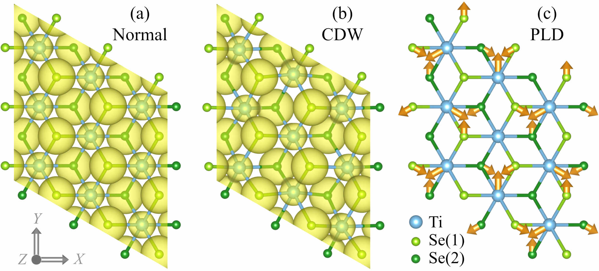
Figure 17: Calculated isosurface of the electronic charge density $\rho(\bm{r})$ in the (a) normal and (b) triple-$\bm{q}$ CDW states. In (b), we assume the self-consistent solution for $V=0.3$ eV shown in Fig. 12. We use the Slater-type orbitals as the atomic orbitals and plot the isosurfaces at an isovalue 0.025 in both (a) and (b). (c) Schematic representation of the periodic lattice displacement (PLD) in the triple-$\bm{q}$ CDW state.

Two remarks are in order. First, the intersite Coulomb interaction $V$ is essential to reproduce the experimental ARPES spectrum in the monolayer TiSe₂ Chen et al. (2015, 2016); Sugawara et al. (2016). When the intersite Coulomb interaction is absent ($V=0$), the calculated band gap and effect of band folding are small and weak in comparison with the experiment. However, the band gap and folding spectrum are enhanced with increasing $V$ and the single-particle spectrum around $V\sim 0.2$ eV may be in good agreement with the ARPES spectrum. Second, since our model omits the spin-orbit coupling, our calculations do not reproduce the spin-orbit splitting of the valence Se 4$p$ bands at the $\Gamma$ point Anderson et al. (1985); Ghafari et al. (2017). The spin-orbit interaction is required for more accurate comparison.

VI.2 Charge Density Distribution

To elucidate the local electronic structure in the triple-$\bm{q}$ CDW state, we calculate the charge density distribution in TiSe₂. In general, the electronic charge density is given by

$$\rho(\bm{r})=\sum_{\bm{k}}\sum_{a}|\psi_{\bm{k},a}(\bm{r})|^{2}f(\varepsilon_{\bm{k},a}),$$ (42)

where $\psi_{\bm{k},a}(\bm{r})$ is the Bloch wave function of band $a$. Here, we do not write the elementary charge $e$ explicitly. Note that the charge density $\rho(\bm{r})$ in Eq. (42) is a density of electrons; the charge distribution of atomic cores (ions) should be added in the evaluation of the total charge density or net electric polarization. In the TB approximation, the Bloch functions are given by the linear combinations of atomic orbitals. The charge density $\rho(\bm{r})$ can then be rewritten as

$$\rho(\bm{r})=\!\sum_{\bm{R}_{i},\bm{R}_{j}}\sum_{\mu\ell,\nu m}\!\braket{c^{{\dagger}}_{i,\mu\ell}c_{j,\nu m}}\phi_{\ell}(\bm{r}\!-\!\bm{R}_{i\mu})\phi_{m}(\bm{r}\!-\!\bm{R}_{j\nu}),$$ (43)

where $c^{({\dagger})}_{i,\mu\ell}$ is the annihilation (creation) operator of an electron on the atomic orbital $\mu\ell$ in the $i$-th unit cell Kaneko and Ohta (2016). Here, we use the Slater-type orbitals as the atomic orbitals $\phi_{\ell}(\bm{r})$, which we have used in the estimation of the overlap integrals in Sec. II C. In the evaluation of Eq. (43), we include the on-site expectation values $\braket{c^{{\dagger}}_{i,\mu\ell}c_{i,\mu m}}$ for all the atoms and the $d$-$p$ bonding contributions $\braket{d^{{\dagger}}_{i,\ell}p_{j,\nu m}}$ between the nearest-neighbor Ti and Se($\nu$) atoms. We omit other (more distant) expectation values because they are negligibly small. In the triple-$\bm{q}$ CDW state, we extend the unit cell as shown in Fig. 4(d) and estimate the expectation values for the four TiSe₂ units in the extended 2$\times$2 unit cell.

Figure 17 shows the calculated charge density distributions in the normal and triple-$\bm{q}$ CDW states. Here, we assume as the CDW state the self-consistent solution for $V=0.3$ eV shown in Fig. 12. Note that the results are qualitatively the same even if we assume $V=0.2$ eV. In the normal state, we find that the isosurface surrounds each atom and the charge densities $\rho(\bm{r})$ around Se sites are larger than those around Ti sites, reflecting the occupation numbers of electrons. We also find that, in the CDW state, the radius of the isosurface surrounding each atom does not change drastically from the normal state, indicating that the CDW state in TiSe₂ is not a site-centered charge order van den Brink and Khomskii (2008) that should have an inequivalent deviation in the on-site electronic occupations. Instead, the deviation in $\rho(\bm{r})$ appears between the Ti and Se sites due to the formation of the bonding orbital (trimer) of the Ti $d$ and two Se $p$ orbitals in the distorted TiSe₆ octahedra. Therefore the trimerization of the Ti and two Se orbitals is the essence in the electronic structure, and the bond-centered CDW van den Brink and Khomskii (2008) is a suitable description of the CDW in TiSe₂.

To illustrate the deviation in the electronic density clearly, Fig. 18(a) shows the difference in the electron density distributions between the CDW and normal states $\Delta\rho(\bm{r})=\rho_{\rm CDW}(\bm{r})-\rho_{\rm N}(\bm{r})$. Clearly, $\Delta\rho(\bm{r})$ exhibits the electric dipole structure in the distorted TiSe₆ octahedra due to the deviation in the electronic density. The schematic representation of the dipole structure is shown in Fig. 18(b), where we only describe the Ti sites, omitting the Se sites, and an arrow indicates the electric polarization in $\Delta\rho(\bm{r})$. We thus find in Fig. 18(b) that the polarization in the Ti sites forms a kagomé network and the dipoles show the structure of clockwise and anticlockwise vortices on the triangles in the kagomé network.

The polarization structure in Fig. 18 given by the electronic density $\rho(\bm{r})$ demonstrates the presence of a vortex-like antiferroelectric structure. In this vortex-like structure shown in Fig. 18(b), we identify the local electric toroidal moment Dubovik and Tugushev (1990); Prosandeev et al. (2006); Guo et al. (2012) along the $Z$-axis at the center of the vortex defined by the three dipoles on the triangle. The clockwise and anticlockwise vortices making opposite axial toroidal vectors can be regarded as the antiferroelectric toroidal network.

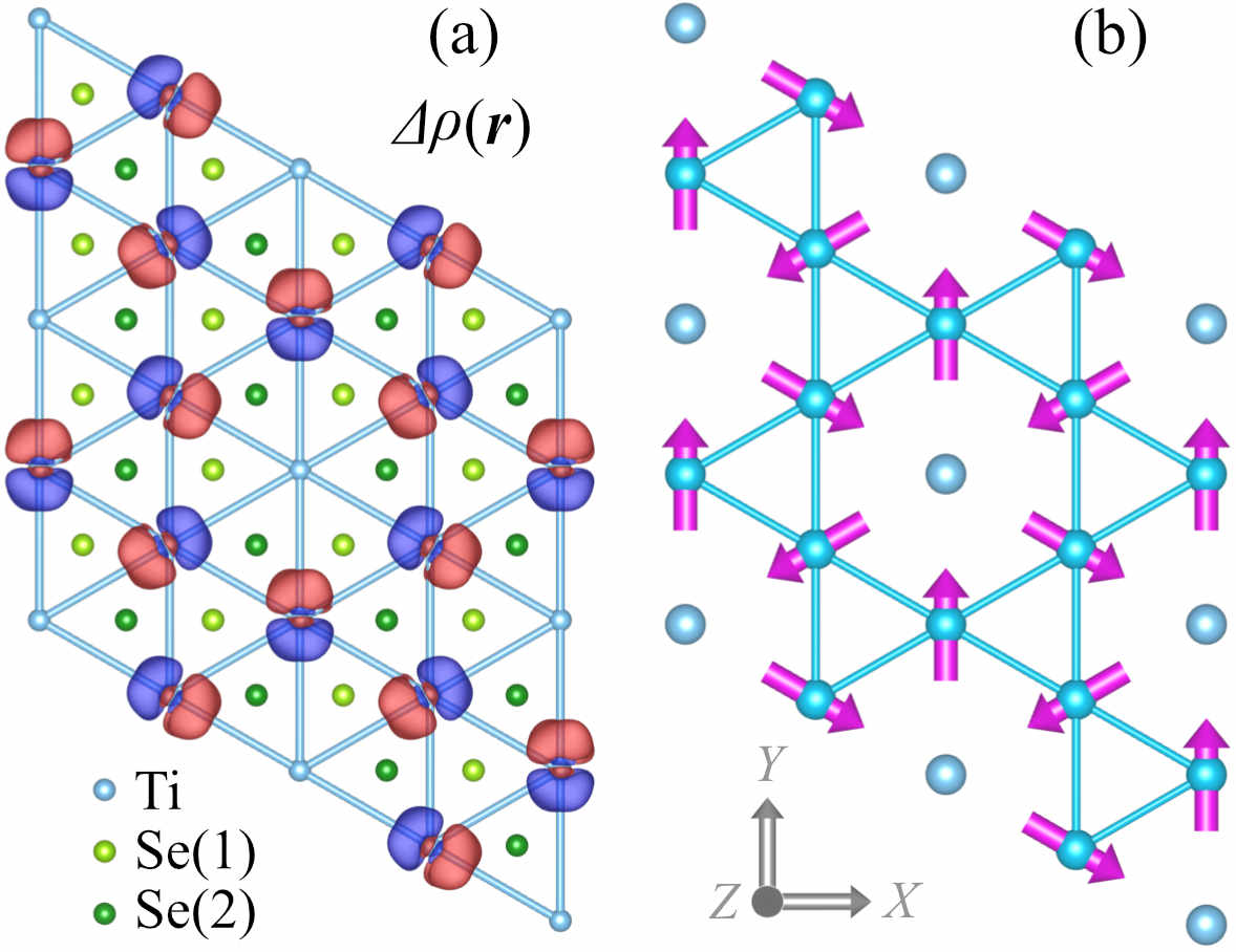
Figure 18: (a) Isosurface of the difference in the electronic charge densities between the triple-$\bm{q}$ CDW and normal states, $\Delta\rho(\bm{r})=\rho_{\rm CDW}(\bm{r})-\rho_{\rm N}(\bm{r})$, where we assume the self-consistent solutions for $V=0.3$ eV given in Fig. 12. We plot the isosurface at an isovalue $\pm$0.007 and the red and blue surfaces indicate the positive and negative part of $\Delta\rho(\bm{r})$, respectively. (b) Schematic representation of the electric polarization in the electronic density shown in (a). An arrow indicates the electric dipole at the Ti sites.

VII Discussion and Summary

Here, we discuss the implications of our results in recent developments in studies of TiSe₂. Recent experimental studies have pointed out the difficulty in the pure excitonic driving force in the formation of the CDW state in TiSe₂, where the PLD is survived even if the excitonic interactions are screened Hildebrand et al. (2016); Novello et al. (2017); Porer et al. (2014); Kogar et al. (2017a). However, these studies have admitted possible contributions of the excitonic correlations to the development in the rigid CDW state of the electron-phonon coupled system Hildebrand et al. (2016); Novello et al. (2017); Porer et al. (2014); Kogar et al. (2017a). Moreover, other experimental results  Monney et al. (2016); Kogar et al. (2017b) have rather supported the cooperative scenario for the CDW formation, as was suggested theoretically van Wezel et al. (2010); Zenker et al. (2013); Watanabe et al. (2015); Kaneko et al. (2015). In this paper, we have shown that the electron-phonon and excitonic interactions work cooperatively with each other to enhance the stability of the triple-$\bm{q}$ CDW state. Our microscopic theory has thus advanced and strengthened the cooperative scenario suggested in simplified models van Wezel et al. (2010); Zenker et al. (2013); Watanabe et al. (2015); Kaneko et al. (2015).

However, the pure phononic mechanism may not be denied completely in our present theory since we have shown the stability of the CDW state without the excitonic interaction, as discussed in Sec. IV. To regard the CDW state in TiSe₂ as an excitonic insulator or excitonic condensation state assertively, we must elucidate the contribution of an excitonic interaction, namely an inter-band Coulomb interaction, in comparison with experiment. As one of the methods of verification, we may suggest the application of time-resolved experiments Möhr-Vorobeva et al. (2011); Rohwer et al. (2011); Hellmann et al. (2012); Mathias et al. (2016); Mor et al. (2017); Werdehausen et al. (2018), where we can make use of the difference in the time scales between the excitonic and phononic systems. In particular, theoretical studies of the photo-induced dynamics for excitonic orders have been investigated in the two-band excitonic insulator models Golež et al. (2016); Murakami et al. (2017). To understand the real materials, however, we need a quantitative microscopic models, for which our theoretical study for TiSe₂ will be proven to be useful. Besides the photo-induced dynamics, responses to other external fields Sugimoto et al. (2016); Sugimoto and Ohta (2016); Matsuura and Ogata (2016) should also be studied theoretically, for which our microscopic model for the CDW state of TiSe₂ will be valuable to elucidate the contributions of the excitonic interaction.

In such studies, we also need to extend our monolayer model to the bulk 1$T$-TiSe₂ model. In the bulk structure, because the bottoms of the conduction band are located at the L points, which are $k_{Z}=\pi/c$ above the M points Zunger and Freeman (1978); Fang et al. (1997), a triple-$\bm{q}$ CDW state with the modulation vector $\bm{q}_{\rm L}=\bm{q}_{\rm M}+(\pi/c)\bm{e}_{Z}$ is anticipated, where the TiSe₂ layers with antiparallel lattice displacements stack alternately along the $Z$-direction, keeping the in-plane structure to be the same as our monolayer triple-$\bm{q}$ structure. Our monolayer studies have thus captured the essential characters of the in-plane structure of the bulk system. However, to understand the bulk 1$T$-TiSe₂ in detail, it is necessary to investigate the roles of the inter-layer coupling carefully.

To conclude, we have investigated the electronic structure and microscopic mechanism of the triple-$\bm{q}$ CDW state in the monolayer TiSe₂ on the basis of the realistic multi-orbital $d$-$p$ model with the electron-phonon coupling and intersite Coulomb (excitonic) interactions. The phononic and excitonic mechanisms of the CDW transition have thus been considered. First, using the first-principles band-structure calculations, we have constructed the tight-binding bands made from the Ti 3$d$ and Se 4$p$ orbitals in the monolayer TiSe₂. From the undistorted band structure, we have shown that the valence-band top at the $\Gamma$ point is characterized by the Se $p$ orbitals and the conduction-band bottom at the M₁, M₂, and M₃ points are characterized by the Ti $d_{xy}$, $d_{yz}$, and $d_{zx}$ orbitals, respectively. Next, we have constructed the electron-phonon coupling in the tight-binding approximation for the transverse phonon modes, of which the softening has been observed experimentally Holt et al. (2001). Taking into account the electron-phonon coupling only, we have shown that the transverse phonon mode softens at the M point of the BZ and that the instability toward the triple-$\bm{q}$ CDW state occurs when the transverse modes at the M₁, M₂, and M₃ points are frozen simultaneously (i.e., representing the phononic mechanism for the triple-$\bm{q}$ CDW state).

Furthermore, we have introduced the intersite Coulomb interaction between the nearest-neighbor Ti and Se atoms, which induces the excitonic instability between the valence Se 4$p$ and conduction Ti 3$d$ bands. We have treated the intersite Coulomb (excitonic) interaction in the mean-field approximation and have shown that the excitonic interaction favors to further stabilize the triple-$\bm{q}$ CDW state caused by the phononic mechanism. We have thus demonstrated that the electron-phonon and excitonic interactions cooperatively stabilize the triple-$\bm{q}$ CDW state in the monolayer TiSe₂. Here, we have also shown the orbital characters of the excitonic order parameters explicitly in the triple-$\bm{q}$ CDW state. Using the mean-field solution for the ground state of the proposed model, we have calculated the single-particle spectrum in the triple-$\bm{q}$ CDW state to reproduce the band folding spectrum observed in the ARPES experiments. To illustrate the electronic structure in the triple-$\bm{q}$ CDW state intuitively, we have also calculated the charge density distribution in real space and have shown that the the bond-type CDW occurs in the monolayer TiSe₂. In addition, we have found out a vortex-like antiferroelectric electron polarization in the kagomé network of Ti atoms.

Appendix A Electron-Phonon Coupling

A.1 Derivation of electron-phonon coupling

Here, following Motizuki et al. Motizuki (1986), we derive the electron-phonon coupling used in Sec. II.3. The electron-phonon coupling is derived from the change in energy when the ions are displaced from their equilibrium positions. Motizuki et al. Motizuki (1986) adopted the Fröhlich approach Fröhlich (1952) in the tight-binding approximation, where the atomic wave functions move rigidly with the ions.

First, for the undistorted system, we write the Bloch wave function in the tight-binding approximation as

$$\phi^{(0)}_{\bm{k},\mu\ell}(\bm{r})=\frac{1}{\sqrt{N}}\sum_{\bm{R}_{i}}e^{i\bm{k}\cdot\bm{R}_{i}}\phi_{\ell}(\bm{r}-\bm{R}_{i\mu}),$$ (44)

where $\phi_{\ell}(\bm{r})$ is the atomic wave function of orbital $\ell$, $\bm{R}_{i\mu}=\bm{R}_{i}+\bm{\tau}_{\mu}$, $\bm{R}_{i}$ is the lattice vector, and $\bm{\tau}_{\mu}$ is the position of atom $\mu$ in the $i$-th unit cell. Using this wave function, we write the transfer integrals in the undistorted system as

$$T^{(0)}_{\mu\ell,\nu m}(\bm{k})=\sum_{\bm{R}_{i}-\bm{R}_{j}}e^{-i\bm{k}\cdot(\bm{R}_{i}-\bm{R}_{j})}T^{(0)}_{i\mu\ell,j\nu m},$$ (45)

where

$$T^{(0)}_{i\mu\ell,j\nu m}\equiv\int d\bm{r}\phi^{*}_{\ell}(\bm{r}-\bm{R}_{i\mu})H_{e}\phi_{m}(\bm{r}-\bm{R}_{j\nu})$$ (46)

and $H_{e}$ represents the one-electron Hamiltonian. The transfer integral $T^{(0)}_{i\mu\ell,j\nu m}$ is a function of $\bm{R}_{n}=\bm{R}_{i}-\bm{R}_{j}$ in the two-center approximation Slater and Koster (1954). When we write $T^{(0)}_{i\mu\ell,j\nu m}=t_{\mu\ell,\nu m}(\bm{R}_{n})$ and $T^{(0)}_{\mu\ell,\nu m}(\bm{k})=t_{\mu\ell,\nu m}(\bm{k})$, the transfer integrals in Eq. (45) become

$$t_{\mu\ell,\nu m}(\bm{k})=\sum_{\bm{R}_{n}}e^{-i\bm{k}\cdot\bm{R}_{n}}t_{\mu\ell,\nu m}(\bm{R}_{n}),$$ (47)

which correspond to Eq. (2) in the main text.

Next, to derive the electron-phonon coupling, we consider the Bloch functions when the ions are displaced from their equilibrium positions. The Bloch wave functions in the distorted system with a lattice displacement $\delta\bm{R}_{i\mu}$ are given by

$$\phi_{\bm{k},\mu\ell}(\bm{r})=\frac{1}{\sqrt{N}}\sum_{\bm{R}_{i}}e^{i\bm{k}\cdot\bm{R}_{i}}\phi_{\ell}(\bm{r}-\bm{R}_{i\mu}-\delta\bm{R}_{i\mu}).$$ (48)

In this case, the transfer integral is not diagonal with respect to $\bm{k}$ and is given by

$$T_{\mu\ell,\nu m}(\bm{k},\bm{k}^{\prime})=\frac{1}{N}\sum_{\bm{R}_{i},\bm{R}_{j}}e^{-i\bm{k}\cdot\bm{R}_{i}}e^{i\bm{k}^{\prime}\cdot\bm{R}_{j}}T_{i\mu\ell,j\nu m},$$ (49)

where

$$T_{i\mu\ell,j\nu m}\equiv\int d\bm{r}\phi^{*}_{\ell}(\bm{r}-\bm{R}_{i\mu}-\delta\bm{R}_{i\mu})H_{e}$$

$$\qquad\qquad\qquad\qquad\times\phi_{m}(\bm{r}-\bm{R}_{j\nu}-\delta\bm{R}_{j\nu}).$$ (50)

Assuming the lattice displacements $\delta\bm{R}_{i\mu}$ are small, we expand the transfer integral to the first-order of $\delta\bm{R}_{i\mu}$ as

$$T_{i\mu\ell,j\nu m}=T^{(0)}_{i\mu\ell,j\nu m}+\left[\bm{\nabla}T_{i\mu\ell,j\nu m}\right]\cdot\left[\delta\bm{R}_{i\mu}-\delta\bm{R}_{j\nu}\right],$$ (51)

where the $\gamma$ $(=x,y,z)$ component of $\bm{\nabla}T_{i\mu\ell,j\nu m}$ is given by Motizuki (1986)

$$\nabla_{\gamma}T_{i\mu\ell,j\nu m}=\left.\left(\frac{\partial}{\partial R^{\gamma}}T_{i\mu\ell,j\nu m}\right)\right|_{\bm{R}=\bm{R}_{i\mu}-\bm{R}_{j\nu}}.$$ (52)

Defining the Fourier transformation of $\delta\bm{R}_{i\mu}$ as

$$\delta\bm{R}_{i\mu}=\frac{1}{\sqrt{N}}\sum_{\bm{q}}e^{i\bm{q}\cdot\bm{R}_{i}}\bm{u}_{\bm{q},\mu},$$ (53)

we obtain the transfer integral $T_{\mu\ell,\nu m}(\bm{k},\bm{k}^{\prime})$ in Eq. (49) as

$$T_{\mu\ell,\nu m}(\bm{k},\bm{k}^{\prime})=T^{(0)}_{\mu\ell,\nu m}(\bm{k})\delta_{\bm{k}^{\prime},\bm{k}}$$

$$+\!\frac{1}{\sqrt{N}}\sum_{\bm{q}}\!\left[\dot{\bm{T}}_{\mu\ell,\nu m}(\bm{k}-\bm{q})\!\cdot\!\bm{u}_{\bm{q},\mu}\!-\!\dot{\bm{T}}_{\mu\ell,\nu m}(\bm{k})\!\cdot\!\bm{u}_{\bm{q},\nu}\right]\!\delta_{\bm{k}^{\prime},\bm{k}-\bm{q}},$$ (54)

where we define

$$\dot{\bm{T}}_{\mu\ell,\nu m}(\bm{k})\equiv\sum_{\bm{R}_{i}-\bm{R}_{j}}e^{-i\bm{k}\cdot(\bm{R}_{i}-\bm{R}_{j})}\left[\bm{\nabla}T_{i\mu\ell,j\nu m}\right].$$ (55)

The first term of $T_{\mu\ell,\nu m}(\bm{k},\bm{k}^{\prime})$ in Eq. (54) is given by the transfer integral in the undistorted system and the second term corresponds to the electron-phonon coupling.

The displacement $\bm{u}_{\bm{q},\mu}$ is in general characterized by the phonon normal coordinates $Q_{\bm{q}\lambda}$ as

$$\bm{u}_{\bm{q},\mu}=\sum_{\lambda}\frac{\bm{\varepsilon}(\bm{q}\lambda,\mu)}{\sqrt{M_{\mu}}}Q_{\bm{q}\lambda},$$ (56)

where $M_{\mu}$ is the mass of atom $\mu$ and $\bm{\varepsilon}(\bm{q}\lambda,\mu)$ is the polarization vector of the phonon of mode $\lambda$ with the phonon frequency $\omega_{0}(\bm{q}\lambda)$. Using the normal coordinates $Q_{\bm{q}\lambda}$, $T_{\mu\ell,\nu m}(\bm{k},\bm{k}^{\prime})$ becomes

$$T_{\mu\ell,\nu m}(\bm{k},\bm{k}^{\prime})= T^{(0)}_{\mu\ell,\nu m}(\bm{k})\delta_{\bm{k}^{\prime},\bm{k}}$$

$$+\frac{1}{\sqrt{N}}\sum_{\bm{q},\lambda}\Bigl{[} \frac{\bm{\varepsilon}(\bm{q}\lambda,\mu)}{\sqrt{M_{\mu}}}\cdot\dot{\bm{T}}_{\mu\ell,\nu m}(\bm{k}-\bm{q})$$

$$- \frac{\bm{\varepsilon}(\bm{q}\lambda,\nu)}{\sqrt{M_{\nu}}}\cdot\dot{\bm{T}}_{\mu\ell,\nu m}(\bm{k})\Bigr{]}Q_{\bm{q}\lambda}\delta_{\bm{k}^{\prime},\bm{k}-\bm{q}}.$$ (57)

Here, defining the coefficient of $Q_{\bm{q}\lambda}$ in the second term of $T_{\mu\ell,\nu m}(\bm{k},\bm{k}^{\prime})$ in Eq. (57) as

$$g^{\lambda}_{\mu\ell,\nu m}(\bm{k},\bm{q}) \equiv\frac{\bm{\varepsilon}(\bm{q}\lambda,\mu)}{\sqrt{M_{\mu}}}\cdot\dot{\bm{T}}_{\mu\ell,\nu m}(\bm{k}-\bm{q})$$

$$\qquad-\frac{\bm{\varepsilon}(\bm{q}\lambda,\nu)}{\sqrt{M_{\nu}}}\cdot\dot{\bm{T}}_{\mu\ell,\nu m}(\bm{k}),$$ (58)

we finally write the transfer integral with the small lattice displacement as

$$T_{\mu\ell,\nu m}(\bm{k},\bm{k}^{\prime}) =t_{\mu\ell,\nu m}(\bm{k})\delta_{\bm{k}^{\prime},\bm{k}}$$

$$+\frac{1}{\sqrt{N}}\sum_{\bm{q},\lambda}g^{\lambda}_{\mu\ell,\nu m}(\bm{k},\bm{q})Q_{\bm{q}\lambda}\delta_{\bm{k}^{\prime},\bm{k}-\bm{q}},$$ (59)

where we also use $t_{\mu\ell,\nu m}(\bm{k})=T^{(0)}_{\mu\ell,\nu m}(\bm{k})$. The second term in Eq. (59) is derived by the lattice distortion and $g^{\lambda}_{\mu\ell,\nu m}(\bm{k},\bm{q})$ corresponds to the electron-phonon coupling for the phonon mode $\lambda$. When we write $\bm{\nabla}T_{i\mu\ell,j\nu m}=\bm{\nabla}t_{\mu\ell,\nu m}(\bm{R}_{n})$ with $\bm{R}_{n}=\bm{R}_{i}-\bm{R}_{j}$, $g^{\lambda}_{\mu\ell,\nu m}(\bm{k},\bm{q})$ becomes

$$g^{\lambda}_{\mu\ell,\nu m}(\bm{k},\bm{q}) =\sum_{\bm{R}_{n}}\Bigl{[}\bm{\nabla}t_{\mu\ell,\nu m}(\bm{R}_{n})\Bigr{]}$$ (60)

$$\cdot\left[\frac{\bm{\varepsilon}(\bm{q}\lambda,\mu)}{\sqrt{M_{\mu}}}e^{-i(\bm{k}-\bm{q})\cdot\bm{R}_{n}}-\frac{\bm{\varepsilon}(\bm{q}\lambda,\nu)}{\sqrt{M_{\nu}}}e^{-i\bm{k}\cdot\bm{R}_{n}}\right].$$

If we assume that the displacement $\bm{u}_{\bm{q},\mu}$ is characterized by a particular normal coordinate $Q_{\bm{q}}$ with

$$\bm{u}_{\bm{q},\mu}=\frac{\bm{\varepsilon}(\bm{q},\mu)}{\sqrt{M_{\mu}}}Q_{\bm{q}},$$ (61)

the transfer integral $T_{\mu\ell,\nu m}(\bm{k},\bm{k}^{\prime})$ in Eq. (59) becomes

$$T_{\mu\ell,\nu m}(\bm{k},\bm{k}^{\prime}) =t_{\mu\ell,\nu m}(\bm{k})\delta_{\bm{k}^{\prime},\bm{k}}$$

$$+\frac{1}{\sqrt{N}}\sum_{\bm{q}}g_{\mu\ell,\nu m}(\bm{k},\bm{q})Q_{\bm{q}}\delta_{\bm{k}^{\prime},\bm{k}-\bm{q}}.$$ (62)

In the main text, we assume that the displacement $\bm{u}_{\bm{q},\mu}$ is characterized only by the normal coordinate of the transverse phonon mode shown in Figs. 4(a)–4(c).

A.2 Susceptibility and phonon softening

Here, we derive the susceptibility $\chi(\bm{q})$ by the second-order perturbation theory with respect to $Q_{\bm{q}}$ following Motizuki et al. Motizuki (1986). The susceptibility $\chi(\bm{q})$ is used in Sec. IV.1 to discuss the phonon softening.

We first transform the transfer integral of Eq. (62) from the atomic orbital $\mu\ell$ representation to the band index $a$ representation, i.e., $\hat{T}^{\prime}=\hat{U}^{(0){\dagger}}\hat{T}\hat{U}^{(0)}$, where the transformation matrix $\hat{U}^{(0)}$ is given by the eigenvectors of the undistorted energy bands $\varepsilon^{(0)}_{\bm{k},a}$. Using the matrix elements $u^{(0)}_{\mu\ell,a}(\bm{k})$ in $\hat{U}^{(0)}$, the transfer integral in the band-index representation is given by

$$T^{\prime}_{a,b}(\bm{k},\bm{k}^{\prime})=\sum_{\mu\ell,\nu m}u^{(0)\,*}_{\mu\ell,a}(\bm{k})T_{\mu\ell,\nu m}(\bm{k},\bm{k}^{\prime})u^{(0)}_{\nu m,b}(\bm{k}^{\prime})$$

$$=\varepsilon^{(0)}_{\bm{k},a}\delta_{\bm{k}^{\prime},\bm{k}}\delta_{a,b}+\frac{1}{\sqrt{N}}\sum_{\bm{q}}V_{ep}(a\bm{k},b\bm{k}-\bm{q})Q_{\bm{q}}\delta_{\bm{k}^{\prime},\bm{k}-\bm{q}},$$ (63)

where $\varepsilon^{(0)}_{\bm{k},a}\delta_{a,b}=\sum_{\mu\ell,\nu m}u^{(0)\,*}_{\mu\ell,a}(\bm{k})t_{\mu\ell,\nu m}(\bm{k})u^{(0)}_{\nu m,b}(\bm{k})$ and

$$V_{ep}(a\bm{k},b\bm{k}\!-\!\bm{q})\equiv\!\sum_{\mu\ell,\nu m}u^{(0)\,*}_{\mu\ell,a}(\bm{k})g_{\mu\ell,\nu m}(\bm{k},\bm{q})u^{(0)}_{\nu m,b}(\bm{k}\!-\!\bm{q}).$$ (64)

Treating the second term of Eq. (63) as perturbation Motizuki (1986), we may write the energy in the second-order perturbation theory as

$$\varepsilon^{(2)}_{\bm{k},a}=\frac{1}{N}\sum_{\bm{q}}\sum_{b}\frac{\left|V_{ep}(a\bm{k},b\bm{k}-\bm{q})Q_{\bm{q}}\right|^{2}}{\varepsilon^{(0)}_{\bm{k},a}-\varepsilon^{(0)}_{\bm{k}-\bm{q},b}},$$ (65)

and the change in the free energy as $\Delta F=2\sum_{\bm{k},a}\varepsilon^{(2)}_{\bm{k},a}f(\varepsilon^{(0)}_{\bm{k},a})$. Using the relation $V^{*}_{ep}(a\bm{k},b\bm{k}-\bm{q})=V_{ep}(b\bm{k}-\bm{q},a\bm{k})$, we find $\Delta F=\sum_{\bm{q}}\Delta F_{\bm{q}}$ with

$$\Delta F_{\bm{q}}=\frac{1}{N}\sum_{\bm{k}}\sum_{a,b}\left|V_{ep}(a\bm{k},b\bm{k}-\bm{q})Q_{\bm{q}}\right|^{2}$$

$$\times\frac{f(\varepsilon^{(0)}_{\bm{k},a})-f(\varepsilon^{(0)}_{\bm{k}-\bm{q},b})}{\varepsilon^{(0)}_{\bm{k},a}-\varepsilon^{(0)}_{\bm{k}-\bm{q},b}}.$$ (66)

Defining the susceptibility as

$$\chi(\bm{q})\equiv\!-\frac{2}{N}\sum_{\bm{k}}\sum_{a,b}\left|V_{ep}(a\bm{k},b\bm{k}\!-\!\bm{q})\right|^{2}\!\frac{f(\varepsilon^{(0)}_{\bm{k},a})\!-\!f(\varepsilon^{(0)}_{\bm{k}-\bm{q},b})}{\varepsilon^{(0)}_{\bm{k},a}\!-\!\varepsilon^{(0)}_{\bm{k}-\bm{q},b}},$$ (67)

we obtain the $\bm{q}$ component of the change in the free energy as

$$\Delta F_{\bm{q}}=-\frac{1}{2}\chi(\bm{q})\left|Q_{\bm{q}}\right|^{2}.$$ (68)

The change in the free energy is not only from the electronic energy $\Delta F_{\bm{q}}=\Delta F^{\rm elec}_{\bm{q}}$ but also from the elastic energy $\Delta F^{\rm elas}_{\bm{q}}$. The change in the elastic energy may be written as

$$\Delta F^{\rm elas}_{\bm{q}}=\frac{1}{2}\omega^{2}_{0}(\bm{q})\left|Q_{\bm{q}}\right|^{2}$$ (69)

with the bare phonon frequency $\omega_{0}(\bm{q})$. The change in the total free energy $\Delta F^{\rm tot}_{\bm{q}}=\Delta F^{\rm elas}_{\bm{q}}+\Delta F^{\rm elec}_{\bm{q}}$ may thus be given by

$$\Delta F^{\rm tot}_{\bm{q}} =\frac{1}{2}\omega^{2}_{0}(\bm{q})\left|Q_{\bm{q}}\right|^{2}-\frac{1}{2}\chi(\bm{q})\left|Q_{\bm{q}}\right|^{2}$$

$$=\frac{1}{2}\omega^{2}(\bm{q})\left|Q_{\bm{q}}\right|^{2},$$ (70)

where we define the effective phonon frequency $\omega(\bm{q})$ as

$$\omega^{2}(\bm{q})=\omega^{2}_{0}(\bm{q})-\chi(\bm{q}).$$ (71)

Therefore, the structural instability of the system may be discussed in terms of this phonon frequency Motizuki (1986), which includes the influence of the electronic system via $\chi(\bm{q})$. We discuss the phonon softening using Eq. (71) in Sec. IV.1.

Appendix B Estimation of the Electron-Phonon Coupling Constant

B.1 Derivatives of the transfer integrals

To estimate the electron-phonon couplings $g^{\lambda}_{\mu\ell,\nu m}(\bm{k},\bm{q})$ defined in Eq. (60), the first derivatives of the transfer integrals $\nabla_{\gamma}t_{\alpha,\beta}(\bm{R})$ are required. Following Motizuki et al. Motizuki (1986), we use the derivatives of the transfer integrals expressed in terms of the Slater-Koster integrals. Here, we write the transfer integral between the $\alpha$ and $\beta$ orbitals located at a distance $\bm{R}$ [$=R\times(l,m,n)$] as $t_{\alpha,\beta}(\bm{R})$ and its derivative in the $\gamma$ (=$x$ or $y$ or $z$) direction as

$$\nabla_{\gamma}t_{\alpha,\beta}(\bm{R})=\lim_{\delta\rightarrow 0}\frac{t_{\alpha,\beta}(\bm{R}+\delta\bm{e}_{\gamma})-t_{\alpha,\beta}(\bm{R})}{\delta},$$ (72)

where $\bm{e}_{\gamma}$ is the unit vector pointing to the $\gamma$ direction. For example, the first derivative in the $\gamma=x$ direction of the transfer integral

$$t_{x,yz}(\bm{R})=lmn\left[\sqrt{3}t(pd\sigma)-2t(pd\pi)\right]$$ (73)

is given by

$$\nabla_{x}t_{x,yz}(\bm{R}) =mn(1-3l^{2})\frac{1}{R}\left[\sqrt{3}t(pd\sigma)-2t(pd\pi)\right]$$

$$+l^{2}mn\left[\sqrt{3}t^{\prime}(pd\sigma)-2t^{\prime}(pd\pi)\right],$$ (74)

where $t^{\prime}(pd\sigma)\!=\![dt(pd\sigma)/dR]$, $t^{\prime}(pd\pi)\!=\![dt(pd\pi)/dR]$, and $(l,m,n)$ are the direction cosines. All the first derivatives $\nabla_{\gamma}t_{\alpha,\beta}(\bm{R})$ expressed in terms of the Slater-Koster integrals are tabulated in Ref. Motizuki (1986).

B.2 Overlap integrals and their derivatives estimated by Slater-type orbitals

To estimate the first derivatives of the transfer integrals $\nabla_{\gamma}t_{\alpha,\beta}(\bm{R})$, we need the first derivatives of the Slater-Koster parameters, e.g., $t^{\prime}(pd\sigma)$ and $t^{\prime}(pd\pi)$. Motizuki and co-workers estimated $t^{\prime}(pd\sigma)$, etc., using the following relation Yoshida and Motizuki (1980); Motizuki (1986):

$$\frac{t^{\prime}(pd\sigma)}{t(pd\sigma)}=\alpha_{\rm c}\frac{s^{\prime}(pd\sigma)}{s(pd\sigma)},\;\;{\rm etc.},$$ (75)

where $s(pd\sigma)$ and $s^{\prime}(pd\sigma)$ are the Slater-Koster parameter for the overlap integral and its first derivative, respectively. Following Motizuki et al. Yoshida and Motizuki (1980); Motizuki (1986), we apply the Slater-type orbitals (STOs) Slater (1930) to estimate the ratio $s^{\prime}(pd\sigma)/s(pd\sigma)$ and $s^{\prime}(pd\pi)/s(pd\pi)$ analytically.

In general, the overlap integral between the $\alpha$ and $\beta$ orbitals located at a distance $\bm{R}$ is given by

$$S(\alpha,\beta)=\int d\bm{r}\phi_{\alpha}(\bm{r})\phi_{\beta}(\bm{r}-\bm{R}),$$ (76)

where $\phi_{\alpha}(\bm{r})$ is the atomic wave function of orbital $\alpha$. In the STO, we assume $R_{n_{\alpha}}(r)=C_{\alpha}r^{n_{\alpha}-1}e^{-\zeta_{\alpha}r}$ as a radial wave function. Thus the atomic orbital $\phi_{\alpha}(\bm{r})$ in the STO is given by Slater (1930); Clementi and Raimondi (1963); Clementi et al. (1967)

$$\phi_{\alpha}(\bm{r})=C_{\alpha}r^{n_{\alpha}-1}e^{-\zeta_{\alpha}r}Y_{l_{\alpha}m_{\alpha}}(\theta,\varphi),$$ (77)

where $n_{\alpha}$, $l_{\alpha}$, and $m_{\alpha}$ are the principal, azimuthal, and magnetic quantum numbers of the $\alpha$ orbital, respectively, and $Y_{l_{\alpha}m_{\alpha}}(\theta,\varphi)$ is the spherical (tesseral) harmonics. $\zeta_{\alpha}$ is the orbital exponent of the $\alpha$ orbital and $C_{\alpha}=(2\zeta_{\alpha})^{n_{\alpha}+\frac{1}{2}}/\sqrt{(2n_{\alpha})!}$ is a normalization constant. The orbital exponents $\zeta_{\alpha}$ are estimated semi-empirically by Slater as the Slater’s rules Slater (1930). However, we use values revised by Clementi et al. Clementi and Raimondi (1963); Clementi et al. (1967) based on the Hartree-Fock method, where the effective principal quantum number $n^{*}_{\alpha}=3.7$ estimated for the 4$p$ ($n_{\alpha}=4$) orbital in the Slater’s rules Slater (1930) becomes an integer in the Clementi’s estimation Clementi and Raimondi (1963); Clementi et al. (1967), and hence the overlap integrals can be estimated analytically. Moreover, in transition-metal and chalcogen atoms, the orbital exponents in the Clementi’s estimations are larger than those in the semi-empirical Slater’s rules Clementi and Raimondi (1963); Clementi et al. (1967), indicating that the more localized atomic orbitals (and thus smaller overlap integrals) are realized when we use the orbital exponents estimated by Clementi et al. Note that we do not write the Bohr radius $a_{0}$ ($\sim 0.529$ Å) explicitly in this section; we rather assume $a_{0}$ as the unit of length.

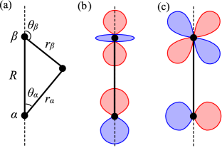
Figure 19: (a) Elliptic coordinate system and examples of the orbitals for the overlap integrals (b) $s(pd\sigma)$ and (c) $s(pd\pi)$.

Although there are several ways to estimate the overlap integrals with the STOs, we adopt the approach of Mulliken et al. Mulliken et al. (1949), where the elliptic coordinate system is employed. As in Fig. 19(a), we assume $\bm{R}=R\bm{e}_{z}$ and the elliptic coordinate system defined by

$$\xi =\frac{r_{\alpha}+r_{\beta}}{R}\>\>\>\>\>\>\left(1\leq\xi\leq\infty\right),$$ (78)

$$\eta =\frac{r_{\alpha}-r_{\beta}}{R}\>\>\>\>\>\>\left(-1\leq\eta\leq 1\right),$$ (79)

$$\varphi =\varphi_{\alpha}=\varphi_{\beta}\>\>\>\>\>\left(0\leq\varphi\leq 2\pi\right),$$ (80)

where $\varphi$ is the azimuthal angle. Using the coordinates $\xi$ and $\eta$, the distance $r_{\alpha}$, $r_{\beta}$ and angle $\theta_{\alpha}$, $\theta_{\beta}$ in Fig. 19(a) are given by

$$r_{\alpha}=\frac{R}{2}\left(\xi+\eta\right),\>\>\>\>\cos\theta_{\alpha}=\frac{\xi\eta+1}{\xi+\eta},$$ (81)

$$r_{\beta}=\frac{R}{2}\left(\xi-\eta\right),\>\>\>\>\>\cos\theta_{\beta}=\frac{\xi\eta-1}{\xi-\eta}.$$ (82)

The volume element in the elliptic coordinate system is given by $d\bm{r}=(R/2)^{3}\left(\xi^{2}-\eta^{2}\right)d\xi d\eta d\varphi$. When we estimate the overlap integrals in the elliptic coordinate system, we usually define Mulliken et al. (1949)

$$p=\frac{R}{2}\left(\zeta_{\alpha}+\zeta_{\beta}\right),\;\;\;t=\frac{\zeta_{\alpha}-\zeta_{\beta}}{\zeta_{\alpha}+\zeta_{\beta}},$$ (83)

for different orbital exponents $\zeta_{\alpha}$ and $\zeta_{\beta}$. Then, the overlap integral $S(\alpha,\beta)$ and its derivative $S^{\prime}(\alpha,\beta)$ [$=dS(\alpha,\beta)/dR$] are written in terms of the parameters $p$ and $t$.

In this paper, we consider the electron-phonon coupling between the nearest-neighbor Ti 3$d$ and Se 4$p$ orbitals, and thus we estimate the overlap integrals $s(pd\sigma)$ and $s(pd\pi)$ for $n_{\alpha}=4$ and $n_{\beta}=3$. As shown in Figs. 19(b) and 19(c), $s(pd\sigma)$ is given by the $\alpha=4p\sigma$ (4$p_{z}$) and $\beta=3d\sigma$ (3$d_{3z^{2}-r^{2}}$) orbitals, and $s(pd\pi)$ is given by the $\alpha=4p\pi$ (4$p_{x}$) and $\beta=3d\pi$ (3$d_{zx}$) orbitals. Using the spherical functions for these orbitals in the elliptic coordinate system, the overlap integrals $s(pd\sigma)=S(4p\sigma,3d\sigma)$ and $s(pd\pi)=S(4p\pi,3d\pi)$ are given, respectively, by

$$S(4p\sigma,3d\sigma) =C_{pd\sigma}p^{8}\int^{\infty}_{1}d\xi\int^{1}_{-1}d\eta(\xi+\eta)^{3}(\xi-\eta)(\xi\eta+1)\left[3(\xi\eta-1)^{2}-(\xi-\eta)^{2}\right]e^{-p(\xi+\eta t)}$$

$$=C_{pd\sigma}p^{8}[A_{7}(3B_{3}-B_{1})+A_{6}(6B_{4}-3B_{2}-B_{0})-3A_{5}(B_{3}+B_{1})-3A_{4}(2B_{6}+B_{2}-B_{0})$$

$$\qquad\quad-3A_{3}(B_{7}-B_{5}-2B_{1})+3A_{2}(B_{6}+B_{4})+A_{1}(B_{7}+3B_{5}-6B_{3})+A_{0}(B_{6}-3B_{4})]$$ (84)

and

$$S(4p\pi,3d\pi) =C_{pd\pi}p^{8}\int^{\infty}_{1}d\xi\int^{1}_{-1}d\eta(\xi+\eta)^{3}(\xi-\eta)(\xi^{2}-1)(1-\eta^{2})(\xi\eta-1)e^{-p(\xi+\eta t)}$$

$$=C_{pd\pi}p^{8}[-A_{7}(B_{3}-B_{1})-A_{6}(2B_{4}-3B_{2}+B_{0})+3A_{5}(B_{3}-B_{1})+A_{4}(2B_{6}-3B_{2}+B_{0})$$

$$\qquad\qquad+A_{3}(B_{7}-3B_{5}+2B_{1})-3A_{2}(B_{6}-B_{4})-A_{1}(B_{7}-3B_{5}+2B_{3})+A_{0}(B_{6}-B_{4})],$$ (85)

where functions $A_{k}$ and $B_{k}$ are defined by

$$A_{k}(p) \equiv\int^{\infty}_{1}\xi^{k}e^{-p\xi}d\xi=e^{-p}\sum^{k}_{\mu=0}\frac{k!}{(k-\mu)!p^{\mu+1}}$$ (86)

and

$$B_{k}(pt) \equiv\int^{1}_{-1}\eta^{k}e^{-pt\eta}d\eta=\sum^{k}_{\mu=0}\frac{k![(-1)^{k-\mu}e^{pt}-e^{-pt}]}{(k-\mu)!(pt)^{\mu+1}},$$ (87)

respectively, and also $C_{pd\sigma}=(\sqrt{210}/80640)(1+t)^{\frac{9}{2}}(1-t)^{\frac{7}{2}}$ and $C_{pd\pi}=(\sqrt{70}/26880)(1+t)^{\frac{9}{2}}(1-t)^{\frac{7}{2}}$.

Using the relations $R[dA_{k}(p)/dR]=-pA_{k+1}(p)$ and $R[dB_{k}(pt))/dR]=-ptB_{k+1}(pt)$, we can also estimate the dimensionless derivative parameter $R\!\times\!s^{\prime}(pd\sigma)=RS^{\prime}(4p\sigma,3d\sigma)$ analytically. Therefore we can evaluate the ratio $s^{\prime}(pd\sigma)/s(pd\sigma)$ from the dimensionless parameter $R\times[s^{\prime}(pd\sigma)/s(pd\sigma)]=RS^{\prime}(4p\sigma,3d\sigma)/S(4p\sigma,3d\sigma)$.

Appendix C Periodic Lattice Distortion and Hamiltonian of the Triple-$\bm{q}$ Structure

Here, we review the triple-$\bm{q}$ structure in TiSe₂, where the transverse phonon modes at the three M points are frozen simultaneously. We also introduce the Hamiltonian in the static triple-$\bm{q}$ structure.

When the transverse phonon modes at the $\bm{q}_{1}$, $\bm{q}_{2}$, and $\bm{q}_{3}$ points are frozen simultaneously, the triple-$\bm{q}$ structure is characterized by the static displacement Motizuki (1986); Suzuki et al. (1985)

$$\delta\bm{R}_{i\mu}=\frac{1}{\sqrt{N}}\sum_{\bm{q}_{j}=\bm{q}_{1},\bm{q}_{2},\bm{q}_{3}}e^{i\bm{q}_{j}\cdot\bm{R}_{i}}\langle\bm{u}_{\bm{q}_{j},\mu}\rangle.$$ (88)

Since the transverse phonon modes are softened at the $\bm{q}_{1}$, $\bm{q}_{2}$, and $\bm{q}_{3}$ points, the direction of $\langle\bm{u}_{\bm{q}_{j},\mu}\rangle$ is perpendicular to its respective wave vector $\bm{q}_{j}$ [see Figs. 4(a)–4(c)]. In practice, $\langle\bm{u}_{\bm{q}_{j},\mu}\rangle$ for Ti atom at $\bm{q}_{1}$, $\bm{q}_{2}$, and $\bm{q}_{3}$ are given by

$$\frac{\langle\bm{u}_{\bm{q}_{1},{\rm Ti}}\rangle}{\sqrt{N}} =u\bm{e}_{Y},$$ (89)

$$\frac{\langle\bm{u}_{\bm{q}_{2},{\rm Ti}}\rangle}{\sqrt{N}} =-\frac{\sqrt{3}}{2}u\bm{e}_{X}-\frac{1}{2}u\bm{e}_{Y},$$ (90)

and

$$\frac{\langle\bm{u}_{\bm{q}_{3},{\rm Ti}}\rangle}{\sqrt{N}} =\frac{\sqrt{3}}{2}u\bm{e}_{X}-\frac{1}{2}u\bm{e}_{Y},$$ (91)

respectively Suzuki et al. (1985); Motizuki (1986), where $u$ is the magnitude of the displacement of Ti atoms. If we assume the ratio $|\bm{u}_{\bm{q}_{j},{\rm Se}}|/|\bm{u}_{\bm{q}_{j},{\rm Ti}}|=1/3$, $\langle\bm{u}_{\bm{q}_{j},\mu}\rangle$ for Se atoms at $\bm{q}_{1}$, $\bm{q}_{2}$, and $\bm{q}_{3}$ are given by

$$\langle\bm{u}_{\bm{q}_{1},{\rm Se1}}\rangle =\langle\bm{u}_{\bm{q}_{1},{\rm Se2}}\rangle=-\langle\bm{u}_{\bm{q}_{1},{\rm Ti}}\rangle/3,$$ (92)

$$\langle\bm{u}_{\bm{q}_{2},{\rm Se1}}\rangle =\langle\bm{u}_{\bm{q}_{2},{\rm Se2}}\rangle=\;\;\;\langle\bm{u}_{\bm{q}_{2},{\rm Ti}}\rangle/3,$$ (93)

and

$$\langle\bm{u}_{\bm{q}_{3},{\rm Se1}}\rangle =\langle\bm{u}_{\bm{q}_{3},{\rm Se2}}\rangle=-\langle\bm{u}_{\bm{q}_{3},{\rm Ti}}\rangle/3,$$ (94)

respectively [see Figs. 4(a)–4(c)]. Note that the sign of $\langle\bm{u}_{\bm{q}_{j},{\rm Se2}}\rangle$ is opposite to the definition of Motizuki et al. Suzuki et al. (1985); Motizuki (1986) since we change the definition of the Se(2) position in the unit cell.

From Eq. (61), the lattice displacement $\bm{u}_{\bm{q}_{j},\mu}$ is characterized by the polarization vector $\bm{\varepsilon}(\bm{q}_{j},\mu)$ and normal coordinate $Q_{\bm{q}_{j}}$ of the transverse phonon mode as $\bm{u}_{\bm{q}_{j},\mu}=\bm{\varepsilon}(\bm{q}_{j},\mu)Q_{\bm{q}_{j}}/\sqrt{M_{\mu}}$. In the static triple-$\bm{q}$ structure, the corresponding expectation value $\langle Q_{\bm{q}_{j}}\rangle$ is given by

$$\langle Q_{\bm{q}_{j}}\rangle=\sqrt{NM^{*}}u\;\;\;(\bm{q}_{j}=\bm{q}_{1},\,\bm{q}_{2},\,\bm{q}_{3}),$$ (95)

where $M^{*}$ is the effective mass of the transverse phonon soft mode Suzuki et al. (1985); Motizuki (1986). From the relation between $\bm{u}_{\bm{q}_{j},\mu}$ and $Q_{\bm{q}_{j}}$, the polarization vector $\bm{\varepsilon}(\bm{q}_{j},\mu)$ of the corresponding transverse mode is given by

$$\bm{\varepsilon}(\bm{q}_{j},\mu)=\sqrt{\frac{M_{\mu}}{M^{*}}}\frac{\braket{\bm{u}_{\bm{q}_{j},\mu}}}{\sqrt{N}u}.$$ (96)

For example, the polarization vectors of the transverse phonon mode at $\bm{q}_{j}=\bm{q}_{1}$ are given by $\bm{\varepsilon}(\bm{q}_{1},{\rm Ti})=\sqrt{M_{\rm Ti}/M^{*}}\bm{e}_{Y}$ and $\bm{\varepsilon}(\bm{q}_{1},{\rm Se1})=\bm{\varepsilon}(\bm{q}_{1},{\rm Se2})=-(1/3)\sqrt{M_{\rm Se}/M^{*}}\bm{e}_{Y}$. From the normalization condition $\sum_{\mu}|\bm{\varepsilon}(\bm{q}_{j},\mu)|^{2}=1$, the effective mass is given by $M^{*}=M_{\rm Ti}+(2/9)M_{\rm Se}$, where we assume $|\bm{u}_{\bm{q}_{j},{\rm Se}}|/|\bm{u}_{\bm{q}_{j},{\rm Ti}}|=1/3$.

When the triple-$\bm{q}$ structure is realized, the band structures are modified through the electron-phonon couplings. Using Eq. (95), the Hamiltonian of the electron-phonon coupling in the static triple-$\bm{q}$ structure becomes

$$\mathcal{H}_{ep}=\sum_{\bm{k},\bm{q}_{j}}\sum_{\mu\ell,\nu m}\bar{g}_{\mu\ell,\nu m}(\bm{k},\bm{q}_{j})uc^{{\dagger}}_{\bm{k},\mu\ell}c_{\bm{k}-\bm{q}_{j},\nu m},$$ (97)

where $\bar{g}_{\mu\ell,\nu m}(\bm{k},\bm{q}_{j})\equiv\sqrt{M^{*}}g_{\mu\ell,\nu m}(\bm{k},\bm{q}_{j})$ and is given by

$$\bar{g}_{\mu\ell,\nu m}(\bm{k},\bm{q}_{j}) =\sum_{\bm{R}_{n}}\left[\bm{\nabla}t_{\mu\ell,\nu m}(\bm{R}_{n})\right]$$ (98)

$$\cdot\left[\bm{n}(\bm{q}_{j},\mu)e^{-i(\bm{k}-\bm{q}_{j})\cdot\bm{R}_{n}}-\bm{n}(\bm{q}_{j},\nu)e^{-i\bm{k}\cdot\bm{R}_{n}}\right],$$

with

$$\bm{n}(\bm{q}_{j},\mu) \equiv\sqrt{M^{*}}\times\frac{\bm{\varepsilon}(\bm{q}_{j},\mu)}{\sqrt{M_{\mu}}}=\frac{\braket{\bm{u}_{\bm{q}_{j},\mu}}}{\sqrt{N}u}.$$ (99)

For example, the vectors $\bm{n}(\bm{q}_{j},\mu)$ at $\bm{q}_{j}=\bm{q}_{1}$ are given by $\bm{n}(\bm{q}_{1},{\rm Ti})=\bm{e}_{Y}$ and $\bm{n}(\bm{q}_{1},{\rm Se1})=\bm{n}(\bm{q}_{1},{\rm Se2})=-(1/3)\bm{e}_{Y}$ in the transverse phonon mode [see Figs. 4(a)–4(c)].

The Hamiltonian of Eq. (97) is not diagonal with respect to $\bm{k}$ in the original BZ without distortion since the transverse phonon modes at $\bm{q}_{1}$, $\bm{q}_{2}$, and $\bm{q}_{3}$ are frozen. Thus, to diagonalize the Hamiltonian, we need to introduce the RBZ, which is 1/4 of the original BZ [see Fig. 2(b)]. In order to write the Hamiltonian simply in the RBZ, we introduce the 11$\times$11 matrices of the transfer integral $[\hat{t}(\bm{k})]_{\mu\ell,\nu m}=t_{\mu\ell,\nu m}(\bm{k})$ and electron-phonon coupling $[\hat{\bar{g}}(\bm{k},\bm{q})]_{\mu\ell,\nu m}=\bar{g}_{\mu\ell,\nu m}(\bm{k},\bm{q})$, and an eleven dimensional vector of the annihilation (creation) operator $[\bm{c}^{({\dagger})}_{\bm{k}}]_{\mu\ell}=c^{({\dagger})}_{\bm{k},\mu\ell}$. Using the matrix and vector formalism, the Hamiltonian of the transfer integral is described as

$$\mathcal{H}_{e}=\sum_{\bm{k}\in{\rm RBZ}}\sum^{3}_{i=0}\bm{c}^{{\dagger}}_{\bm{k}-\bm{q}_{i}}\hat{t}(\bm{k}-\bm{q}_{i})\bm{c}_{\bm{k}-\bm{q}_{i}}$$ (100)

within the RBZ, where we define $\bm{q}_{0}=\bm{0}$. Similarly, the Hamiltonian of the electron-phonon coupling in Eq. (97) is now

$$\mathcal{H}_{ep}=\sum_{\bm{k}\in{\rm RBZ}}\sum^{3}_{i=0}\sum^{3}_{j=1}\bm{c}^{{\dagger}}_{\bm{k}-\bm{q}_{i}}[\hat{\bar{g}}(\bm{k}-\bm{q}_{i},\bm{q}_{j})u]\bm{c}_{\bm{k}-\bm{q}_{i}-\bm{q}_{j}}.$$ (101)

Notice that due to $\hat{\bar{g}}^{{\dagger}}(\bm{k},\bm{q}_{j})=\hat{\bar{g}}(\bm{k}-\bm{q}_{j},\bm{q}_{j})=\hat{\bar{g}}(\bm{k}_{j},\bm{q}_{j})$, $\mathcal{H}_{ep}$ in Eq. (101) satisfies the Hermitian property. When we define a 44 dimensional row vector as $\bar{\bm{c}}^{{\dagger}}_{\bm{k}}=(\,\bm{c}^{{\dagger}}_{\bm{k}}\;\bm{c}^{{\dagger}}_{\bm{k}_{1}}\;\bm{c}^{{\dagger}}_{\bm{k}_{2}}\;\bm{c}^{{\dagger}}_{\bm{k}_{3}}\,)$ with $\bm{k}_{i}=\bm{k}-\bm{q}_{i}$, the Hamiltonians $\mathcal{H}_{e}$ and $\mathcal{H}_{ep}$ are written as

$$\mathcal{H}^{ep}_{cdw}=\mathcal{H}_{e}+\mathcal{H}_{ep}=\sum_{\bm{k}\in{\rm RBZ}}\bar{\bm{c}}^{{\dagger}}_{\bm{k}}\hat{\mathcal{H}}^{ep}_{\bm{k}}\bar{\bm{c}}_{\bm{k}},$$ (102)

with the 44$\times$44 matrix

$$\hat{\mathcal{H}}^{ep}_{\bm{k}}=\begin{pmatrix}\hat{t}(\bm{k})&\hat{\bar{g}}(\bm{k},\bm{q}_{1})u&\hat{\bar{g}}(\bm{k},\bm{q}_{2})u&\hat{\bar{g}}(\bm{k},\bm{q}_{3})u\\ &\hat{t}(\bm{k}_{1})&\hat{\bar{g}}(\bm{k}_{1},\bm{q}_{3})u&\hat{\bar{g}}(\bm{k}_{1},\bm{q}_{2})u\\ &&\hat{t}(\bm{k}_{2})&\hat{\bar{g}}(\bm{k}_{2},\bm{q}_{1})u\\ &\rm{H.C.}&&\hat{t}(\bm{k}_{3})\end{pmatrix},$$ (103)

where we use the relations $\bm{q}_{1}+\bm{q}_{2}+\bm{q}_{3}=\bm{0}$ and $\bm{c}^{{\dagger}}_{\bm{k}-2\bm{q}_{j}}=\bm{c}^{{\dagger}}_{\bm{k}}$. Thus we can calculate the energy bands in the presence of the triple-$\bm{q}$ structure by diagonalizing the Hamiltonian $\hat{\mathcal{H}}^{ep}_{\bm{k}}$ in the RBZ.

Appendix D Mean-Field Approximation for the Intersite Coulomb Interaction

Here, we summarize the details of the mean-field approximation for the intersite Coulomb interaction, which leads to the excitonic instability in TiSe₂. We assume the following intersite Coulomb interaction

$$\mathcal{H}_{ee}\!=\!\frac{1}{N}\!\sum_{\bm{k},\bm{k}^{\prime},\bm{q}}\sum_{\ell,\nu m}\!V^{dp}_{\ell,\nu m}(\bm{k}\!-\!\bm{k}^{\prime})d^{{\dagger}}_{\bm{k},\ell}d_{\bm{k}^{\prime},\ell}p^{{\dagger}}_{\bm{k}^{\prime}\!-\bm{q},\nu m}p_{\bm{k}\!-\bm{q},\nu m}.$$ (104)

In TiSe₂, the top of the valence Se $p$ bands and the bottom of the conduction Ti $d$ bands are located in the BZ at the momenta separated by $\bm{q}_{j}=\bm{q}_{1}$, $\bm{q}_{2}$, and $\bm{q}_{3}$. Thus the order parameter defined by the expectation value $\braket{p^{{\dagger}}_{\bm{k}-\bm{q}_{j},\nu m}d_{\bm{k},\ell}}\neq 0$ is anticipated. We therefore introduce the following mean-field approximation:

$$\sum_{\bm{q}} d^{{\dagger}}_{\bm{k},\ell}d_{\bm{k}^{\prime},\ell}p^{{\dagger}}_{\bm{k}^{\prime}-\bm{q},\nu m}p_{\bm{k}-\bm{q},\nu m}$$

$$\sim -\sum_{\bm{q}_{j}}\braket{p^{{\dagger}}_{\bm{k}^{\prime}-\bm{q}_{j},\nu m}d_{\bm{k}^{\prime},\ell}}d^{{\dagger}}_{\bm{k},\ell}p_{\bm{k}-\bm{q}_{j},\nu m}$$

$$-\sum_{\bm{q}_{j}}\braket{d^{{\dagger}}_{\bm{k},\ell}p_{\bm{k}-\bm{q}_{j},\nu m}}p^{{\dagger}}_{\bm{k}^{\prime}-\bm{q}_{j},\nu m}d_{\bm{k}^{\prime},\ell}$$

$$+\sum_{\bm{q}_{j}}\braket{p^{{\dagger}}_{\bm{k}^{\prime}-\bm{q}_{j},\nu m}d_{\bm{k}^{\prime},\ell}}\braket{d^{{\dagger}}_{\bm{k},\ell}p_{\bm{k}-\bm{q}_{j},\nu m}},$$ (105)

where $\langle\cdots\rangle$ denotes the grand canonical average at temperature $T$ with respect to the mean-field Hamiltonian. Note that we assume the spin-singlet $d$-$p$ hybridization because we also take into account the electron-phonon coupling, which is known to induce the spin-singlet hybridization Kaneko et al. (2015). The spin-triplet hybridization is expected to occur in the presence of the Hund’s-like exchange interaction Kaneko and Ohta (2014). Here, we introduce the excitonic order parameter

$$\Delta^{dp}_{\ell,\nu m}(\bm{k},\bm{q}_{j})\equiv-\frac{1}{N}\sum_{\bm{k}^{\prime}}V^{dp}_{\ell,\nu m}(\bm{k}-\bm{k}^{\prime})\braket{p^{{\dagger}}_{\bm{k}^{\prime}-\bm{q}_{j},\nu m}d_{\bm{k}^{\prime},\ell}},$$ (106)

and thus the mean-field Hamiltonian $\mathcal{H}^{\rm MF}_{ee}$ is given by

$$\mathcal{H}^{\rm MF}_{ee} =\mathcal{H}_{cdw}^{ex}+E^{ex}_{0},$$ (107)

where

$$\mathcal{H}_{cdw}^{ex} \equiv\sum_{\bm{k},\bm{q}_{j}}\sum_{\ell,\nu m}\Delta^{dp}_{\ell,\nu m}(\bm{k},\bm{q}_{j})d^{{\dagger}}_{\bm{k},\ell}p_{\bm{k}-\bm{q}_{j},\nu m}+{\mathrm{H.c.}}$$ (108)

and

$$E^{ex}_{0} \equiv-\sum_{\bm{k},\bm{q}_{j}}\sum_{\ell,\nu m}\Delta^{dp}_{\ell,\nu m}(\bm{k},\bm{q}_{j})\braket{d^{{\dagger}}_{\bm{k},\ell}p_{\bm{k}-\bm{q}_{j},\nu m}}.$$ (109)

Since the mean-field Hamiltonian is not diagonal with respect to $\bm{k}$ in the original BZ, we also need to apply the RBZ introduced in the Appendix C. We use the 5$\times$6 matrix representation of the order parameter $[\hat{\Delta}(\bm{k},\bm{q}_{j})]_{\ell,\nu m}=\Delta^{dp}_{\ell,\nu m}(\bm{k},\bm{q}_{j})$, the five dimensional vector representation of the annihilation (creation) operators of the Ti $d$ orbitals $[\bm{d}^{({\dagger})}_{\bm{k}}]_{\ell}=d^{({\dagger})}_{\bm{k},\ell}$, and the six dimensional vector representation of the two Se($\nu$) $p$ orbitals $[\bm{p}^{({\dagger})}_{\bm{k}}]_{\nu m}=p^{({\dagger})}_{\bm{k},\nu m}$. In this matrix and vector representation, the mean-field Hamiltonian $\mathcal{H}_{cdw}^{ex}$ in the RBZ is written as

$$\mathcal{H}_{cdw}^{ex}=\!\sum_{\bm{k}\in{\rm RBZ}}\sum_{i=0}^{3}\sum_{j=1}^{3}\bm{d}^{{\dagger}}_{\bm{k}-\bm{q}_{i}}\hat{\Delta}(\bm{k}\!-\!\bm{q}_{i},\bm{q}_{j})\bm{p}_{\bm{k}-\bm{q}_{i}-\bm{q}_{j}}\!+{\mathrm{H.c.}}$$ (110)

When we define the eleven dimensional vector $\bm{c}^{{\dagger}}_{\bm{k}_{i}}=(\bm{d}^{{\dagger}}_{\bm{k}_{i}}\>\bm{p}^{{\dagger}}_{\bm{k}_{i}})$ in $\bar{\bm{c}}^{{\dagger}}_{\bm{k}}=(\,\bm{c}^{{\dagger}}_{\bm{k}}\;\bm{c}^{{\dagger}}_{\bm{k}_{1}}\;\bm{c}^{{\dagger}}_{\bm{k}_{2}}\;\bm{c}^{{\dagger}}_{\bm{k}_{3}})$, the Hamiltonian of Eq. (110) is summarized as

$$\mathcal{H}_{cdw}^{ex}=\sum_{\bm{k}\in{\rm RBZ}}\bar{\bm{c}}^{{\dagger}}_{\bm{k}}\hat{\mathcal{H}}^{ex}_{\bm{k}}\bar{\bm{c}}_{\bm{k}}$$ (111)

with the 44$\times$44 matrix

$$\hat{\mathcal{H}}^{ex}_{\bm{k}}=\left(\begin{array}[]{c c | c c | c c | c c}\hat{0}&\hat{0}&\hat{0}&\hat{\Delta}(\bm{k},\bm{q}_{1})&\hat{0}&\hat{\Delta}(\bm{k},\bm{q}_{2})&\hat{0}&\hat{\Delta}(\bm{k},\bm{q}_{3})\\ \hat{0}&\hat{0}&\hat{\Delta}^{{\dagger}}(\bm{k}_{1},\bm{q}_{1})&\hat{0}&\hat{\Delta}^{{\dagger}}(\bm{k}_{2},\bm{q}_{2})&\hat{0}&\hat{\Delta}^{{\dagger}}(\bm{k}_{3},\bm{q}_{3})&\hat{0}\\ \hline\cr\hat{0}&\hat{\Delta}(\bm{k}_{1},\bm{q}_{1})&\hat{0}&\hat{0}&\hat{0}&\hat{\Delta}(\bm{k}_{1},\bm{q}_{3})&\hat{0}&\hat{\Delta}(\bm{k}_{1},\bm{q}_{2})\\ \hat{\Delta}^{{\dagger}}(\bm{k},\bm{q}_{1})&\hat{0}&\hat{0}&\hat{0}&\hat{\Delta}^{{\dagger}}(\bm{k}_{2},\bm{q}_{3})&\hat{0}&\hat{\Delta}^{{\dagger}}(\bm{k}_{3},\bm{q}_{2})&\hat{0}\\ \hline\cr\hat{0}&\hat{\Delta}(\bm{k}_{2},\bm{q}_{2})&\hat{0}&\hat{\Delta}(\bm{k}_{2},\bm{q}_{3})&\hat{0}&\hat{0}&\hat{0}&\hat{\Delta}(\bm{k}_{2},\bm{q}_{1})\\ \hat{\Delta}^{{\dagger}}(\bm{k},\bm{q}_{2})&\hat{0}&\hat{\Delta}^{{\dagger}}(\bm{k}_{1},\bm{q}_{3})&\hat{0}&\hat{0}&\hat{0}&\hat{\Delta}^{{\dagger}}(\bm{k}_{3},\bm{q}_{1})&\hat{0}\\ \hline\cr\hat{0}&\hat{\Delta}(\bm{k}_{3},\bm{q}_{3})&\hat{0}&\hat{\Delta}(\bm{k}_{3},\bm{q}_{2})&\hat{0}&\hat{\Delta}(\bm{k}_{3},\bm{q}_{1})&\hat{0}&\hat{0}\\ \hat{\Delta}^{{\dagger}}(\bm{k},\bm{q}_{3})&\hat{0}&\hat{\Delta}^{{\dagger}}(\bm{k}_{1},\bm{q}_{2})&\hat{0}&\hat{\Delta}^{{\dagger}}(\bm{k}_{2},\bm{q}_{1})&\hat{0}&\hat{0}&\hat{0}\\ \end{array}\right).$$ (120)

In the same way, we need to introduce the RBZ for the order parameter $\Delta^{dp}_{\ell,\nu m}(\bm{k},\bm{q}_{j})$ in Eq. (106). In the RBZ, the order parameter $\Delta^{dp}_{\ell,\nu m}(\bm{k}_{i},\bm{q}_{j})$ in $\hat{\mathcal{H}}^{ex}_{\bm{k}}$ is given by

$$\Delta^{dp}_{\ell,\nu m}(\bm{k}_{i},\bm{q}_{j})=-\frac{1}{N}\sum_{\bm{k}^{\prime}\in{\rm RBZ}}\sum_{i^{\prime}=0}^{3}V^{dp}_{\ell,\nu m}(\bm{k}_{i}-\bm{k}^{\prime}_{i^{\prime}})$$

$$\times\braket{p^{{\dagger}}_{\bm{k}^{\prime}-\bm{q}_{i^{\prime}}-\bm{q}_{j},\nu m}d_{\bm{k}^{\prime}-\bm{q}_{i^{\prime}},\ell}}.$$ (121)

Once $\hat{\mathcal{H}}^{ex}_{\bm{k}}$ is diagonalized in the RBZ, the annihilation (creation) operator of the $\mu\ell$ atomic orbital is given by the unitary transformation

$$c^{({\dagger})}_{\bm{k}-\bm{q}_{j},\mu\ell}=\sum_{a}u^{(*)}_{\bm{q}_{j}\mu\ell,a}(\bm{k})\gamma^{({\dagger})}_{\bm{k},a},$$ (122)

where $\gamma^{({\dagger})}_{\bm{k},a}$ is the annihilation (creation) operator of the electron in the band $\varepsilon_{\bm{k},a}$, and $u^{(*)}_{\bm{q}_{j}\mu\ell,a}(\bm{k})$ is the matrix element in the transformation matrix $\hat{U}$ ($\hat{U}^{{\dagger}}$) between the atomic orbital $\mu\ell$ with $\bm{q}_{j}$ and band index $a$. Using this transformation, the order parameter in Eq. (121) becomes

$$\Delta^{dp}_{\ell,\nu m}(\bm{k}_{i},\bm{q}_{j})=-\frac{1}{N}\sum_{\bm{k}^{\prime}\in{\rm RBZ}}\sum_{i^{\prime}=0}^{3}\sum_{a}V^{dp}_{\ell,\nu m}(\bm{k}_{i}-\bm{k}^{\prime}_{i^{\prime}})$$

$$\times u^{*}_{\bm{q}_{i^{\prime}}+\bm{q}_{j}p(\nu)m,a}(\bm{k}^{\prime})u_{\bm{q}_{i^{\prime}}d\ell,a}(\bm{k}^{\prime})f(\varepsilon_{\bm{k}^{\prime},a}),$$ (123)

where we write Ti atom as $d$ and Se($\nu$) atom as $p(\nu)$ in $u_{\bm{q}_{j}\mu\ell,a}(\bm{k})$, and $f(\varepsilon_{\bm{k},a})=\braket{\gamma^{{\dagger}}_{\bm{k},a}\gamma_{\bm{k},a}}$ is the Fermi distribution function. Equation (123) corresponds to the gap equation of the excitonic order. The order parameter $\hat{\Delta}(\bm{k}_{i},\bm{q}_{j})$ is optimized self-consistently. Finally, the energy term $E^{ex}_{0}$ in the RBZ is given by

$$E^{ex}_{0}=-2\sum_{\bm{k}\in{\rm RBZ}}\sum_{i=0}^{3}\sum_{j=1}^{3}\sum_{\ell,\nu m}\sum_{a}\Delta^{dp}_{\ell,\nu m}(\bm{k}_{i},\bm{q}_{j})$$

$$\times u^{*}_{\bm{q}_{i}d\ell,a}(\bm{k})u_{\bm{q}_{i}+\bm{q}_{j}p(\nu)m,a}(\bm{k})f(\varepsilon_{\bm{k},a}).$$ (124)

Note that the prefactor 2 in Eq. (124) is for the spin degrees of freedom.

Appendix E Single-Particle Spectrum

Here, we introduce the single-particle excitation spectrum $A(\bm{k},\omega)$ in the triple-$\bm{q}$ CDW state. The single-particle spectrum $A(\bm{k},\omega)$ is given by the sum of the spectra over the atomic orbitals $\mu\ell$ as

$$A(\bm{k},\omega)=-\frac{1}{\pi}\sum_{\mu\ell}{\rm Im}\>G_{\mu\ell}(\bm{k},\omega)$$ (125)

with the $\mu\ell$ component given as

$$G_{\mu\ell}(\bm{k},\omega)=-i\int^{\infty}_{0}dte^{i(\omega+i\eta)t}\braket{\{c_{\bm{k},\mu\ell}(t),c^{{\dagger}}_{\bm{k},\mu\ell}\}},$$ (126)

where $c_{\bm{k},\mu\ell}(t)$ is the Heisenberg representation of $c_{\bm{k},\mu\ell}$, $\{A,B\}=AB+BA$, and $\eta\rightarrow 0^{+}$. The finite $\eta$ value corresponds to the broadening factor of the spectrum.

When the Hamiltonian is diagonalized in the RBZ for the triple-$\bm{q}$ CDW state, the annihilation (creation) operators of the component $\mu\ell$ are given by $c^{({\dagger})}_{\bm{k},\mu\ell}=\sum_{a}u^{(*)}_{\bm{q}_{0}\mu\ell,a}(\bm{k})\gamma^{({\dagger})}_{\bm{k},a}$. Note that the wave-vector $\bm{k}$ in $A(\bm{k},\omega)$ is defined in the unfolded original BZ and hence we only consider the $\bm{q}_{0}$ components in the $u_{\bm{q}_{j}\mu\ell,a}$. By the transformation of the operators, the single-particle Green’s function $G_{\mu\ell}(\bm{k},\omega)$ becomes

$$G_{\mu\ell}(\bm{k},\omega)= -i\sum_{a}|u_{\bm{q}_{0}\mu\ell,a}(\bm{k})|^{2}$$

$$\times\int^{\infty}_{0}dte^{i(\omega+i\eta)t}\braket{\{\gamma_{\bm{k},a}(t),\gamma^{{\dagger}}_{\bm{k},a}\}}.$$ (127)

In the one-body approximation, the integral part in the Green’s function of Eq. (127) is given by

$$-i\int^{\infty}_{0}dte^{i(\omega+i\eta)t}\braket{\{\gamma_{\bm{k},a}(t),\gamma^{{\dagger}}_{\bm{k},a}\}}=\frac{1}{\omega\!-\!\varepsilon_{\bm{k},a}\!+\!i\eta}$$ (128)

and the Green’s function $G_{\mu\ell}(\bm{k},\omega)$ is

$$G_{\mu\ell}(\bm{k},\omega)=\sum_{a}\frac{|u_{\bm{q}_{0}\mu\ell,a}(\bm{k})|^{2}}{\omega-\varepsilon_{\bm{k},a}+i\eta}.$$ (129)

From Eqs. (125) and (129), the single-particle spectrum $A(\bm{k},\omega)$ is given by

$$A(\bm{k},\omega) =-\frac{1}{\pi}\sum_{\mu\ell}\sum_{a}{\rm Im}\left[\frac{|u_{\bm{q}_{0}\mu\ell,a}(\bm{k})|^{2}}{\omega-\varepsilon_{\bm{k},a}+i\eta}\right]$$

$$=\sum_{\mu\ell}\sum_{a}|u_{\bm{q}_{0}\mu\ell,a}(\bm{k})|^{2}\delta(\omega-\varepsilon_{\bm{k},a}),$$ (130)

where we use ${\rm Im}\left[1/(\omega-\varepsilon_{\bm{k},a}+i\eta)\right]=-\pi\delta(\omega-\varepsilon_{\bm{k},a})$ in the limit of $\eta\rightarrow 0^{+}$ in the second equation. In Fig. 16, we assume a finite broadening parameter $\eta$ in the first equation of Eq. (130).

References

- Wilson and Yoffe (1969) J. Wilson and A. Yoffe, Adv. Phys. 18, 193 (1969).
- Chhowalla et al. (2013) M. Chhowalla, H. S. Shin, G. Eda, L.-J. Li, K. P. Loh, and H. Zhang, Nat. Chem. 5, 263 (2013).
- Motizuki (1986) K. Motizuki, Structural Phase Transitions in Layered Transition Metal Compounds (Reidel, Dordrecht, 1986).
- Rossnagel (2011) K. Rossnagel, J. Phys.: Condens. Matter 23, 213001 (2011).
- Zunger and Freeman (1978) A. Zunger and A. J. Freeman, Phys. Rev. B 17, 1839 (1978).
- Fang et al. (1997) C. M. Fang, R. A. de Groot, and C. Haas, Phys. Rev. B 56, 4455 (1997).
- Woo et al. (1976) K. C. Woo, F. C. Brown, W. L. McMillan, R. J. Miller, M. J. Schaffman, and M. P. Sears, Phys. Rev. B 14, 3242 (1976).
- Di Salvo et al. (1976) F. J. Di Salvo, D. E. Moncton, and J. V. Waszczak, Phys. Rev. B 14, 4321 (1976).
- Holt et al. (2001) M. Holt, P. Zschack, H. Hong, M. Y. Chou, and T.-C. Chiang, Phys. Rev. Lett. 86, 3799 (2001).
- Grüner (1988) G. Grüner, Rev. Mod. Phys. 60, 1129 (1988).
- Grüner (2000) G. Grüner, Density Waves in Solids (Perseus, New York, 2000).
- Wilson et al. (1974) J. A. Wilson, F. J. Di Salvo, and S. Mahajan, Phys. Rev. Lett. 32, 882 (1974).
- Wilson et al. (1975) J. A. Wilson, F. J. Di Salvo, and S. Mahajan, Adv. Phys. 24, 117 (1975).
- Morosan et al. (2006) E. Morosan, H. W. Zandbergen, B. S. Dennis, J. W. G. Bos, Y. Onose, T. Klimczuk, A. P. Ramirez, N. P. Ong, and R. J. Cava, Nat. Phys. 2, 544 (2006).
- Morosan et al. (2007) E. Morosan, L. Li, N. P. Ong, and R. J. Cava, Phys. Rev. B 75, 104505 (2007).
- Li et al. (2007a) S. Y. Li, G. Wu, X. H. Chen, and L. Taillefer, Phys. Rev. Lett. 99, 107001 (2007a).
- Morosan et al. (2010) E. Morosan, K. E. Wagner, L. L. Zhao, Y. Hor, A. J. Williams, J. Tao, Y. Zhu, and R. J. Cava, Phys. Rev. B 81, 094524 (2010).
- Giang et al. (2010) N. Giang, Q. Xu, Y. S. Hor, A. J. Williams, S. E. Dutton, H. W. Zandbergen, and R. J. Cava, Phys. Rev. B 82, 024503 (2010).
- Luo et al. (2016a) H. Luo, K. Yan, I. Pletikosic, W. Xie, B. F. Phelan, T. Valla, and R. J. Cava, J. Phys. Soc. Jpn. 85, 064705 (2016a).
- Song et al. (2016) Y. J. Song, M. J. Kim, W. G. Jung, B.-J. Kim, and J.-S. Rhyee, Phys. Status Solidi B 253, 1517 (2016).
- Sato et al. (2017) K. Sato, T. Noji, T. Hatakeda, T. Kawamata, M. Kato, and Y. Koike, J. Phys. Soc. Jpn. 86, 104701 (2017).
- Kusmartseva et al. (2009) A. F. Kusmartseva, B. Sipos, H. Berger, L. Forró, and E. Tutiš, Phys. Rev. Lett. 103, 236401 (2009).
- Joe et al. (2014) Y. I. Joe, X. M. Chen, P. Ghaemi, K. D. Finkelstein, G. A. de La Peña, Y. Gan, J. C. T. Lee, S. Yuan, J. Geck, G. J. MacDougall, T. C. Chiang, S. L. Cooper, E. Fradkin, and P. Abbamonte, Nat. Phys. 10, 421 (2014).
- Li et al. (2016) L. J. Li, E. C. T. O’Farrell, K. P. Loh, G. Eda, B. Özyilmaz, and A. H. C. Neto, Nature (London) 592, 185 (2016).
- Luo et al. (2016b) H. Luo, W. Xie, J. Tao, I. Pletikosic, T. Valla, G. S. Sahasrabudhe, G. Osterhoudt, E. Sutton, K. S. Burch, E. M. Seibel, J. W. Krizan, Y. Zhu, and R. J. Cava, Chem. Mater. 28, 1927 (2016b).
- Wilson (1977) J. A. Wilson, Solid State Commun. 22, 551 (1977).
- Traum et al. (1978) M. M. Traum, G. Margaritondo, N. V. Smith, J. E. Rowe, and F. J. Di Salvo, Phys. Rev. B 17, 1836 (1978).
- Keldysh and Kopeav (1965) L. V. Keldysh and Y. V. Kopeav, Sov. Phys. Solid State 6, 2219 (1965).
- Des Cloizeaux (1965) J. Des Cloizeaux, J. Phys. Chem. Solids 26, 259 (1965).
- Jérome et al. (1967) D. Jérome, T. M. Rice, and W. Kohn, Phys. Rev. 158, 462 (1967).
- Kohn (1967) W. Kohn, Phys. Rev. Lett. 19, 439 (1967).
- Halperin and Rice (1968a) B. I. Halperin and T. M. Rice, Rev. Mod. Phys. 40, 755 (1968a).
- Halperin and Rice (1968b) B. I. Halperin and T. M. Rice, Solid State Physics, Vol. 21 (Academic Press, New York, 1968) p. 115.
- Seki et al. (2011) K. Seki, R. Eder, and Y. Ohta, Phys. Rev. B 84, 245106 (2011).
- Kaneko et al. (2012) T. Kaneko, K. Seki, and Y. Ohta, Phys. Rev. B 85, 165135 (2012).
- Ejima et al. (2014) S. Ejima, T. Kaneko, Y. Ohta, and H. Fehske, Phys. Rev. Lett. 112, 026401 (2014).
- Kuneš and Augustinský (2014a) J. Kuneš and P. Augustinský, Phys. Rev. B 89, 115134 (2014a).
- Kuneš and Augustinský (2014b) J. Kuneš and P. Augustinský, Phys. Rev. B 90, 235112 (2014b).
- Kuneš (2015) J. Kuneš, J. Phys.: Condens. Matter 27, 333201 (2015).
- Nasu et al. (2016) J. Nasu, T. Watanabe, M. Naka, and S. Ishihara, Phys. Rev. B 93, 205136 (2016).
- Di Salvo et al. (1986) F. Di Salvo, C. Chen, R. Fleming, J. Waszczak, R. Dunn, S. Sunshine, and J. A. Ibers, J. Less-Common Met. 116, 51 (1986).
- Wakisaka et al. (2009) Y. Wakisaka, T. Sudayama, K. Takubo, T. Mizokawa, M. Arita, H. Namatame, M. Taniguchi, N. Katayama, M. Nohara, and H. Takagi, Phys. Rev. Lett. 103, 026402 (2009).
- (43) T. Kaneko, T. Toriyama, T. Konishi, and Y. Ohta, Phys. Rev. B 87, 035121 (2013); 87, 199902(E) (2013).
- Seki et al. (2014) K. Seki, Y. Wakisaka, T. Kaneko, T. Toriyama, T. Konishi, T. Sudayama, N. L. Saini, M. Arita, H. Namatame, M. Taniguchi, N. Katayama, M. Nohara, H. Takagi, T. Mizokawa, and Y. Ohta, Phys. Rev. B 90, 155116 (2014).
- Yamada et al. (2016) T. Yamada, K. Domon, and Y. Ōno, J. Phys. Soc. Jpn. 85, 053703 (2016).
- Lu et al. (2017) Y. F. Lu, H. Kono, T. I. Larkin, A. W. Rost, T. Takayama, A. V. Boris, B. Keimer, and H. Takagi, Nat. Commun. 8, 14408 (2017).
- Pillo et al. (2000) T. Pillo, J. Hayoz, H. Berger, F. Lévy, L. Schlapbach, and P. Aebi, Phys. Rev. B 61, 16213 (2000).
- Kidd et al. (2002) T. E. Kidd, T. Miller, M. Y. Chou, and T.-C. Chiang, Phys. Rev. Lett. 88, 226402 (2002).
- Cercellier et al. (2007) H. Cercellier, C. Monney, F. Clerc, C. Battaglia, L. Despont, M. G. Garnier, H. Beck, P. Aebi, L. Patthey, H. Berger, and L. Forró, Phys. Rev. Lett. 99, 146403 (2007).
- Li et al. (2007b) G. Li, W. Z. Hu, D. Qian, D. Hsieh, M. Z. Hasan, E. Morosan, R. J. Cava, and N. L. Wang, Phys. Rev. Lett. 99, 027404 (2007b).
- Qian et al. (2007) D. Qian, D. Hsieh, L. Wray, E. Morosan, N. L. Wang, Y. Xia, R. J. Cava, and M. Z. Hasan, Phys. Rev. Lett. 98, 117007 (2007).
- Zhao et al. (2007) J. F. Zhao, H. W. Ou, G. Wu, B. P. Xie, Y. Zhang, D. W. Shen, J. Wei, L. X. Yang, J. K. Dong, M. Arita, H. Namatame, M. Taniguchi, X. H. Chen, and D. L. Feng, Phys. Rev. Lett. 99, 146401 (2007).
- Monney et al. (2009) C. Monney, H. Cercellier, F. Clerc, C. Battaglia, E. F. Schwier, C. Didiot, M. G. Garnier, H. Beck, P. Aebi, H. Berger, L. Forró, and L. Patthey, Phys. Rev. B 79, 045116 (2009).
- Monney et al. (2010a) C. Monney, E. F. Schwier, M. G. Garnier, N. Mariotti, C. Didiot, H. Beck, P. Aebi, H. Cercellier, J. Marcus, C. Battaglia, H. Berger, and A. N. Titov, Phys. Rev. B 81, 155104 (2010a).
- Monney et al. (2010b) C. Monney, E. F. Schwier, M. G. Garnier, N. Mariotti, C. Didiot, H. Cercellier, J. Marcus, H. Berger, A. N. Titov, H. Beck, and P. Aebi, New J. Phys. 12, 125019 (2010b).
- May et al. (2011) M. M. May, C. Brabetz, C. Janowitz, and R. Manzke, Phys. Rev. Lett. 107, 176405 (2011).
- Cazzaniga et al. (2012) M. Cazzaniga, H. Cercellier, M. Holzmann, C. Monney, P. Aebi, G. Onida, and V. Olevano, Phys. Rev. B 85, 195111 (2012).
- Monney et al. (2012a) C. Monney, G. Monney, P. Aebi, and H. Beck, Phys. Rev. B 85, 235150 (2012a).
- Monney et al. (2012b) C. Monney, G. Monney, P. Aebi, and H. Beck, New J. Phys. 14, 075026 (2012b).
- Monney et al. (2015) G. Monney, C. Monney, B. Hildebrand, P. Aebi, and H. Beck, Phys. Rev. Lett. 114, 086402 (2015).
- Hughes (1977) H. P. Hughes, J. Phys. C: Solid State Phys. 10, L319 (1977).
- White and Lucovsky (1977) R. M. White and G. Lucovsky, Il Nuovo Cimento B 38, 280 (1977).
- Yoshida and Motizuki (1980) Y. Yoshida and K. Motizuki, J. Phys. Soc. Jpn. 49, 898 (1980).
- Takaoka and Motizuki (1980) Y. Takaoka and K. Motizuki, J. Phys. Soc. Jpn. 49, 1838 (1980).
- Motizuki et al. (1981a) K. Motizuki, N. Suzuki, Y. Yoshida, and Y. Takaoka, Solid State Commun. 40, 995 (1981a).
- Motizuki et al. (1981b) K. Motizuki, Y. Yoshida, and Y. Takaoka, Physica B+C 105, 357 (1981b).
- Suzuki et al. (1984) N. Suzuki, A. Yamamoto, and K. Motizuki, Solid State Commun. 49, 1039 (1984).
- Suzuki et al. (1985) N. Suzuki, A. Yamamoto, and K. Motizuki, J. Phys. Soc. Jpn. 54, 4668 (1985).
- Calandra and Mauri (2011) M. Calandra and F. Mauri, Phys. Rev. Lett. 106, 196406 (2011).
- Bianco et al. (2015) R. Bianco, M. Calandra, and F. Mauri, Phys. Rev. B 92, 094107 (2015).
- Duong et al. (2015) D. L. Duong, M. Burghard, and J. C. Schön, Phys. Rev. B 92, 245131 (2015).
- Fu et al. (2016) Z.-G. Fu, Z.-Y. Hu, Y. Yang, Y. Lu, F.-W. Zheng, and P. Zhang, RSC Adv. 6, 76972 (2016).
- Singh et al. (2017) B. Singh, C.-H. Hsu, W.-F. Tsai, V. M. Pereira, and H. Lin, Phys. Rev. B 95, 245136 (2017).
- Hellgren et al. (2017) M. Hellgren, J. Baima, R. Bianco, M. Calandra, F. Mauri, and L. Wirtz, Phys. Rev. Lett. 119, 176401 (2017).
- Holy et al. (1977) J. A. Holy, K. C. Woo, M. V. Klein, and F. C. Brown, Phys. Rev. B 16, 3628 (1977).
- Sugai et al. (1980) S. Sugai, K. Murase, S. Uchida, and S. Tanaka, Solid State Commun. 35, 433 (1980).
- Snow et al. (2003) C. S. Snow, J. F. Karpus, S. L. Cooper, T. E. Kidd, and T.-C. Chiang, Phys. Rev. Lett. 91, 136402 (2003).
- Barath et al. (2008) H. Barath, M. Kim, J. F. Karpus, S. L. Cooper, P. Abbamonte, E. Fradkin, E. Morosan, and R. J. Cava, Phys. Rev. Lett. 100, 106402 (2008).
- Goli et al. (2012) P. Goli, J. Khan, D. Wickramaratne, R. K. Lake, and A. A. Balandin, Nano Lett. 12, 5941 (2012).
- Duong et al. (2017) D. L. Duong, G. Ryu, A. Hoyer, C. Lin, M. Burghard, and K. Kern, ACS Nano 11, 1034 (2017).
- Stirling et al. (1976) W. G. Stirling, B. Dorner, J. D. N. Cheeke, and J. Revelli, Solid State Commun. 18, 931 (1976).
- Wakabayashi et al. (1978) N. Wakabayashi, H. G. Smith, K. C. Woo, and F. C. Brown, Solid State Commun. 28, 923 (1978).
- Jaswal (1979) S. S. Jaswal, Phys. Rev. B 20, 5297 (1979).
- Weber et al. (2011) F. Weber, S. Rosenkranz, J.-P. Castellan, R. Osborn, G. Karapetrov, R. Hott, R. Heid, K.-P. Bohnen, and A. Alatas, Phys. Rev. Lett. 107, 266401 (2011).
- Maschek et al. (2016) M. Maschek, S. Rosenkranz, R. Hott, R. Heid, M. Merz, D. A. Zocco, A. H. Said, A. Alatas, G. Karapetrov, S. Zhu, J. van Wezel, and F. Weber, Phys. Rev. B 94, 214507 (2016).
- van Wezel et al. (2010) J. van Wezel, P. Nahai-Williamson, and S. S. Saxena, Phys. Rev. B 81, 165109 (2010).
- Zenker et al. (2013) B. Zenker, H. Fehske, H. Beck, C. Monney, and A. R. Bishop, Phys. Rev. B 88, 075138 (2013).
- Watanabe et al. (2015) H. Watanabe, K. Seki, and S. Yunoki, Phys. Rev. B 91, 205135 (2015).
- Kaneko et al. (2015) T. Kaneko, B. Zenker, H. Fehske, and Y. Ohta, Phys. Rev. B 92, 115106 (2015).
- Peng et al. (2015) J.-P. Peng, J.-Q. Guan, H.-M. Zhang, C.-L. Song, L. Wang, K. He, Q.-K. Xue, and X.-C. Ma, Phys. Rev. B 91, 121113 (2015).
- Chen et al. (2015) P. Chen, Y.-H. Chan, X.-Y. Fang, Y. Zhang, M.-Y. Chou, S.-K. Mo, Z. Hussain, A.-V. Fedorov, and T.-C. Chiang, Nat. Commun. 6, 8943 (2015).
- Sugawara et al. (2016) K. Sugawara, Y. Nakata, R. Shimizu, P. Han, T. Hitosugi, T. Sato, and T. Takahashi, ACS Nano 10, 1341 (2016).
- Chen et al. (2016) P. Chen, Y.-H. Chan, M.-H. Wong, X.-Y. Fang, M. Y. Chou, S.-K. Mo, Z. Hussain, A.-V. Fedorov, and T.-C. Chiang, Nano Lett. 16, 6331 (2016).
- Fang et al. (2017) X.-Y. Fang, H. Hong, P. Chen, and T.-C. Chiang, Phys. Rev. B 95, 201409 (2017).
- Note (1) The crystal structures and the isosurfaces are visualized using VESTA, K. Momma and F. Izumi, J. Appl. Crystallogr. 44 1272 (2011).
- Riekel (1976) C. Riekel, J. Solid State Chem. 17, 389 (1976).
- Blaha et al. (2001) P. Blaha, K. Schwarz, G. Madsen, D. Kvasnicka, and J. Luitz, WIEN2k, An Augmented Plane Wave + Local Orbitals Program for Calculating Crystal Properties (Technical Universität Wien, Austria, 2001).
- Note (2) We optimize the internal coordinates of Se ions in the trigonal structure (space group ) with the lattice constants and Å, where Å is large enough to get rid of the interlayer connections. In the self-consistent calculations, we adopt the GGA Perdew et al. (1996) and use 88 -points in the irreducible part of the BZ, assuming the muffin-tin radii () of 2.28 (Ti) and 2.28 (Se) bohr and the plane-wave cutoff of .
- Kamimura et al. (1969) H. Kamimura, S. Sugano, and Y. Tanabe, Ligand Field Theory and Its Applications (Syokabo, Tokyo, 1969).
- Monney et al. (2011) C. Monney, C. Battaglia, H. Cercellier, P. Aebi, and H. Beck, Phys. Rev. Lett. 106, 106404 (2011).
- Slater and Koster (1954) J. C. Slater and G. F. Koster, Phys. Rev. 94, 1498 (1954).
- Note (3) In the DFT band calculation, we use the optimized crystal structure obtained in Sec. II.1. In the self-consistent calculations, we use 416 -points in the irreducible part of the BZ, assuming the muffin-tin radii () of 2.41 (Ti) and 2.41 (Se) bohr and the plane-wave cutoff of .
- Perdew et al. (1996) J. P. Perdew, K. Burke, and M. Ernzerhof, Phys. Rev. Lett. 77, 3865 (1996).
- Kuneš et al. (2010) J. Kuneš, R. Arita, P. Wissgott, A. Toschi, H. Ikeda, and K. Held, Comp. Phys. Commun. 181, 1888 (2010).
- Mostofi et al. (2008) A. A. Mostofi, J. R. Yates, Y.-S. Lee, I. Souza, D. Vanderbilt, and N. Marzari, Comp. Phys. Commun. 178, 685 (2008).
- Slater (1930) J. C. Slater, Phys. Rev. 36, 57 (1930).
- Clementi and Raimondi (1963) E. Clementi and D.-L. Raimondi, J. Chem. Phys. 38, 2686 (1963).
- Clementi et al. (1967) E. Clementi, D. Raimondi, and W. Reinhardt, J. Chem. Phys. 47, 1300 (1967).
- van Wezel (2011) J. van Wezel, Europhys. Lett. 96, 67011 (2011).
- Blöchl et al. (1994) P. E. Blöchl, O. Jepsen, and O. K. Andersen, Phys. Rev. B 49, 16223 (1994).
- Anderson et al. (1985) O. Anderson, R. Manzke, and M. Skibowski, Phys. Rev. Lett. 55, 2188 (1985).
- Ghafari et al. (2017) A. Ghafari, L. Petaccia, and C. Janowitz, Appl. Surf. Sci. 396, 1649 (2017).
- Kaneko and Ohta (2016) T. Kaneko and Y. Ohta, Phys. Rev. B 94, 125127 (2016).
- van den Brink and Khomskii (2008) J. van den Brink and D. I. Khomskii, J. Phys.: Condens. Matter 20, 434217 (2008).
- Dubovik and Tugushev (1990) V. Dubovik and V. Tugushev, Phys. Rep 187, 145 (1990).
- Prosandeev et al. (2006) S. Prosandeev, I. Ponomareva, I. Kornev, I. Naumov, and L. Bellaiche, Phys. Rev. Lett. 96, 237601 (2006).
- Guo et al. (2012) L. Y. Guo, M. H. Li, Q. W. Ye, B. X. Xiao, and H. L. Yang, Eur. Phys. J. B 85, 208 (2012).
- Hildebrand et al. (2016) B. Hildebrand, T. Jaouen, C. Didiot, E. Razzoli, G. Monney, M.-L. Mottas, A. Ubaldini, H. Berger, C. Barreteau, H. Beck, D. R. Bowler, and P. Aebi, Phys. Rev. B 93, 125140 (2016).
- Novello et al. (2017) A. M. Novello, M. Spera, A. Scarfato, A. Ubaldini, E. Giannini, D. R. Bowler, and C. Renner, Phys. Rev. Lett. 118, 017002 (2017).
- Porer et al. (2014) M. Porer, U. Leierseder, J.-M. Ménard, H. Dachraoui, L. Mouchliadis, I. Perakis, U. Heinzmann, J. Demsar, K. Rossnagel, and R. Huber, Nat. Mater. 13, 857 (2014).
- Kogar et al. (2017a) A. Kogar, G. A. de la Pena, S. Lee, Y. Fang, S. X.-L. Sun, D. B. Lioi, G. Karapetrov, K. D. Finkelstein, J. P. C. Ruff, P. Abbamonte, and S. Rosenkranz, Phys. Rev. Lett. 118, 027002 (2017a).
- Monney et al. (2016) C. Monney, M. Puppin, C. W. Nicholson, M. Hoesch, R. T. Chapman, E. Springate, H. Berger, A. Magrez, C. Cacho, R. Ernstorfer, and M. Wolf, Phys. Rev. B 94, 165165 (2016).
- Kogar et al. (2017b) A. Kogar, M. S. Rak, S. Vig, A. A. Husain, F. Flicker, Y. I. Joe, L. Venema, G. J. MacDougall, T. C. Chiang, E. Fradkin, J. van Wezel, and P. Abbamonte, Science 358, 1314 (2017b).
- Möhr-Vorobeva et al. (2011) E. Möhr-Vorobeva, S. L. Johnson, P. Beaud, U. Staub, R. De Souza, C. Milne, G. Ingold, J. Demsar, H. Schaefer, and A. Titov, Phys. Rev. Lett. 107, 036403 (2011).
- Rohwer et al. (2011) T. Rohwer, S. Hellmann, M. Wiesenmayer, C. Sohrt, A. Stange, B. Slomski, A. Carr, Y. Liu, L. M. Avila, M. Kalläne, S. Mathias, L. Kipp, K. Rossnagel, and M. Bauer, Nature (London) 471, 490 (2011).
- Hellmann et al. (2012) S. Hellmann, T. Rohwer, M. Kalläne, K. Hanff, C. Sohrt, A. Stange, A. Carr, M. Murnane, H. Kapteyn, L. Kipp, M. Bauer, and K. Rossnagel, Nat. Commun. 3, 1069 (2012).
- Mathias et al. (2016) S. Mathias, S. Eich, J. Urbancic, S. Michael, A. V. Carr, S. Emmerich, A. Stange, T. Popmintchev, T. Rohwer, M. Wiesenmayer, A. Ruffing, S. Jakobs, S. Hellmann, P. Matyba, C. Chen, L. Kipp, M. Bauer, H. C. Kapteyn, H. C. Schneider, K. Rossnagel, M. M. Murnane, and M. Aeschlimann, Nat. Commun. 7, 12902 (2016).
- Mor et al. (2017) S. Mor, M. Herzog, D. Golež, P. Werner, M. Eckstein, N. Katayama, M. Nohara, H. Takagi, T. Mizokawa, C. Monney, and J. Stähler, Phys. Rev. Lett. 119, 086401 (2017).
- Werdehausen et al. (2018) D. Werdehausen, T. Takayama, M. Höppner, G. Albrecht, A. W. Rost, Y. Lu, D. Manske, H. Takagi, and S. Kaiser, Sci. Adv. 4, eaap8652 (2018).
- Golež et al. (2016) D. Golež, P. Werner, and M. Eckstein, Phys. Rev. B 94, 035121 (2016).
- Murakami et al. (2017) Y. Murakami, D. Golež, M. Eckstein, and P. Werner, Phys. Rev. Lett. 119, 247601 (2017).
- Sugimoto et al. (2016) K. Sugimoto, T. Kaneko, and Y. Ohta, Phys. Rev. B 93, 041105 (2016).
- Sugimoto and Ohta (2016) K. Sugimoto and Y. Ohta, Phys. Rev. B 94, 085111 (2016).
- Matsuura and Ogata (2016) H. Matsuura and M. Ogata, J. Phys. Soc. Jpn. 85, 093701 (2016).
- Fröhlich (1952) H. Fröhlich, Proc. R. Soc. A 215, 291 (1952).
- Mulliken et al. (1949) R. Mulliken, C. Rieke, D. Orloff, and H. Orloff, J. Chem. Phys. 17, 1248 (1949).
- Kaneko and Ohta (2014) T. Kaneko and Y. Ohta, Phys. Rev. B 90, 245144 (2014).