Entanglement Entropy for D3-, M2- and M5-brane backgrounds

Abstract

In the context of the gauge/gravity duality applications, we study and compute the entanglement entropy of gauge theories corresponding to string/M theories on D3-, M2- and M5-brane backgrounds. This is achieved using the Ryu-Takayanagi formula. We obtain the entanglement entropy for the general cases of the D3-, M2- and M5-brane backgrounds and also for the near horizon AdS limit, as well as the non-conformal flat space limit in each case.

1 Introduction

The thermal entropy of black holes obey an area-law established by Bekenstein Bekenstein:1973ur and Hawking Hawking:1976de and it was re-obtained using string theory in Strominger:1996sh . The relation between entropy and temperature of black holes and string theory were further investigated in Gubser:1996de where the entropy and temperature of non-extremal black 3-branes were calculated.

Soon after, Maldacena proposed the AdS/CFT correspondence maldacena1 conjecturing a duality between string/M-theory in anti-de Sitter space in $(d+2)$ dimensions times a compact space $\cal M$ with supercorformal field theories in $(d+1)$-dimensional flat spacetime. The black hole entropy in de Sitter space as well as the quantum entanglement were then analysed using the AdS/CFT correspondence in Hawking:2000da . In that work, it was found that the quantum entanglement entropy can also be viewed as the entropy of the thermal Rindler particles near the horizon, thereby avoiding reference to the unobservable region behind the horizon, which is the usual situation of the entanglement entropy.

A major advance in the calculation of the entanglement entropy was achieved by Ryu-Takayanagi (RT) Ryu:2006bv . As we know, one can define the entanglement entropy $S_{A}$ in a gauge theory on $\mathbb{R}^{(1,d)}$ for a subsystem $A$ that has an arbitrary $(d-1)$-dimensional boundary $\partial A\subset\mathbb{R}^{d}$. In this set up, the proposal for the entanglement entropy is given by:

$$S_{A}=\frac{\text{Area}(\gamma_{A})}{4G_{N}^{(d+2)}},$$ (1)

where $\gamma_{A}$ denotes the $d$ dimensional static minimal surface in $AdS_{d+2}$ whose boundary coincides with the boundary of region $A$ ($\partial A=\partial\gamma_{A}$) and $G_{N}^{(d+2)}$ is the $(d+2)-$dimensional Newton’s constant.

Further developments on the entanglement entropy including the application to non-conformal cases were discussed in Ryu:2006ef . Specifically, those non-conformal cases considered in Ryu:2006ef were the ones corresponding to dilatonic D2- and NS5-branes as the gravity backgrounds. In our paper we work with non-dilatonic extremal brane solutions and we will only obtain non-conformal cases when we go beyond the strong coupling limit.

With the aim of understanding the time-dependence of the entanglement entropy for generic quantum field theories, a covariant holographic entanglement entropy proposal was presented in Hubeny:2007xt . In ref. Faraggi:2007fu the holographic entanglement entropy and phase transitions at finite temperature were studied.

Geometric entropy, which is related to entanglement entropy with a double Wick rotation, was introduced in Fujita:2008zv as a parameter of order in confinement/deconfinement transitions, as expected, this entropy becomes discontinuous at the Hagedorn temperature both in free $\mathcal{N}=4$ super Yang-Mills, and its supergravity duals.

As opposed to the thermal entropy, the entanglement entropy is non-vanishing at zero temperature. Therefore we can employ it to probe the quantum properties of the ground state for a given quantum system Nishioka:2009un .

With the motivation of quantifying the degree of superhorizon correlations that are generated by the cosmological expansion, a computation of entanglement entropy for quantum field theories in de Sitter space was presented in Maldacena:2012xp . Other authors Bea:2015fja have calculated entanglement entropy for other CFTs that were obtained as a result of finding new compactification spaces in the dual string theory on $AdS_{3}\times\mathcal{M}$. This entanglement entropy were considered as a way of characterizing these new CFTs . A proposal on how to derive properties of the bulk geometry from the starting point of abstract quantum states in a Hilbert space using the entanglement entropy was presented in Cao:2016mst . In refs. Mishra:2015cpa ; Mishra:2016yor ; Ghosh:2017ygi the holographic entanglement entropy has been calculated for the boosted blackbrane up to second order.

In our paper we compute and analyze the entanglement entropy of large $N$ gauge theories holographically dual to string/M-theories on D3-, M2- and M5-brane supergravity backgrounds. First, we derive analytically this entropy for the limit geometries $AdS_{5}\times S^{5}$, $AdS_{4}\times S^{7}$ and $AdS_{7}\times S^{4}$ of the brane cases, confirming the results obtained in Ryu:2006bv , and also for the Minkowski-like limit geometries of these same brane background spaces. The case of the D3-brane was discussed recently in connection with the open-closed string duality Niarchos:2017cdz .

As it is know, the curvature of $AdS$ spaces are constant. On the contrary, the curvature of the general non-dilatonic extremal solutions of supergravity, i.e D3-, M2- and M5-brane background spaces, are not constant. So it would be interesting to analyze how possible geometric transitions (i.e. at zero temperature) could occur when one goes from one geometric regime to the other which are both contained in these background spaces. For such aim, in this work we also do a numerical study comparing the entanglement entropy in some brane-background spaces with their asymptotic regimes.

This paper is organized as follows, in sec. 2 we study the entanglement entropy in the D3-brane background. We do the same in sec. 3 and sec. 4, for M2- and M5-brane backgrounds, respectively. Finally, in sec. 5, we present some conclusions on this paper and some ideas for possible future works.

2 Entanglement entropy for the D3-brane background

Consider a quantum field theory or a many-body system defined on $(d+1)$-dimensional region $A\cup B$ ($A\cap B=\emptyset$), see fig. 1, where $A$ and $B$ are $d$-dimensional space-like manifolds. Then, the entanglement entropy $S_{A}$ is defined as the Von Neumann entropy $S_{A}$ of the reduced density matrix when we take the partial trace with respect to the degrees of freedom inside $B$. The entanglement entropy $S_{A}$ measures how the subsystems $A$ and $B$ are correlated with each other. In other words, this is the entropy for an observer in $A$ who is not accessible to $B$.

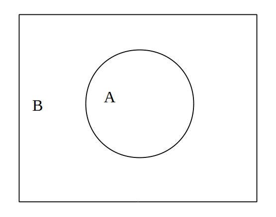
Figure 1: Subsystems $A$ and $B$ in the space of a field theory.

From the point of view of holography, this entanglement entropy can be seen as a geometric object in the bulk. This object is the minimal area surface in the bulk that has the same boundary of that of the subsystem $A$.

As a first example we do the computation of the entanglement entropy ($S_{A}$) corresponding to the space-time generated by a large $N$ number of coincident D3-branes. The invariant measure for this geometry is: Horowitz:1991cd ; Gubser:1998bc

$$ds^{2}=dx^{\mu}dx^{\nu}g_{\mu\nu}=\left(1+\frac{R^{4}}{r^{4}}\right)^{-1/2}(-dt^{2}+dx_{3}^{2})+\left(1+\frac{R^{4}}{r^{4}}\right)^{1/2}(dr^{2}+r^{2}d\Omega^{2}_{5}),$$ (2)

where $x^{\mu}=(t,x^{a},r,\theta_{b})$, with $a=1,2,3$ and $b=1,2...5$, are the space-time coordinates, $g_{\mu\nu}$ is the space-time metric, $R=(4\pi gNl_{s}^{4})^{1/4}$, $dx_{3}^{2}$ is the euclidean line element in $\mathbb{R}^{3}$ and $d\Omega^{2}_{5}$ is the line element on the 5-sphere which only depends on $\theta_{b}$ coordinates.

2.1 Rectangular strip

Throughout this paper we choose an infinite rectangular strip as the subsystem $A$. This rectangular strip will be defined for each background geometry in the next sections. The style of the computations performed in this paper were inspired in those that can be found in Fischler:2013gsa .

For a 3-dimensional ($d=3$) subsystem $A\in\mathbb{R}^{3}$ we choose the following rectangular strip region:

$$X\equiv x^{1}\in\left[-\frac{l}{2},\frac{l}{2}\right]\,\,\,,\,\,\,x^{2},x^{3}\in\left[-\frac{L}{2},\frac{L}{2}\right].$$ (3)

The corresponding extremal surface is translationally invariant along $x^{2}$, $x^{3}$ and the profile in the bulk is given by $x^{1}\equiv X(r)$. The area of this surface is given by

$$\mathcal{A}=\int d^{3}\sigma\sqrt{det(G_{\alpha\beta})},$$ (4)

where $G_{\alpha\beta}\equiv\partial_{\alpha}x^{\mu}\partial_{\beta}x^{\nu}g_{\mu\nu}$ is the induced metric on the surface $\gamma_{A}$ in the bulk. We took the parametrization of $\gamma_{A}$ as : $\sigma_{1}=r$, $\sigma_{2}=x^{2}$, $\sigma_{3}=x^{3}$. As a result we have:

$$\mathcal{A}=L^{2}\int\frac{dr}{f(r)}\sqrt{\frac{X^{\prime 2}}{f(r)}+f(r)},$$ (5)

where $f(r)=\sqrt{1+R^{4}/r^{4}}$, and $X^{\prime}\equiv dX/dr$.

From the functional area (5) we obtain the equation for the profile $X(r)$ that makes the area $A$ extremal:

$$\frac{dX}{dr}=\pm\frac{f^{5/2}(r)}{\sqrt{f^{3}(r_{a})-f^{3}(r)}},$$ (6)

where that $r_{a}$ is the closest approach of the extremal surface (see fig.2) to the origin of $r$ coordinate.

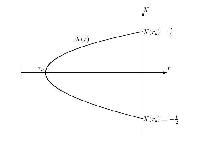
Figure 2: Profile $X(r)$ of the $\gamma_{A}$ surface with boundary conditions.

Such surface has two branches, joined smoothly at $r=r_{a}$, where $X=0$ and $X^{\prime}\rightarrow\infty$. Additionally we choose an UV cut-off value $r_{b}$ that defines the next boundary condition for the profile $X(r)$:

$$X(r_{b})=\pm\frac{l}{2},$$ (7)

With this condition we integrate (6) to obtain the width of the strip:

$$\frac{l}{2}=\int_{r_{a}}^{r_{b}}dr\frac{f^{5/2}(r)}{\sqrt{f^{3}(r_{a})-f^{3}(r)}}.$$ (8)

Note that $r_{a}$ can be determined in terms of $l$ and $r_{b}$ from this last equation. After substitution of eq.(6) into eq.(5) and considering the limits of integration defined in eq.(8) we finally get the extremal area:

$$\mathcal{A}=L^{2}\int_{r_{a}}^{r_{b}}dr\frac{f^{3/2}(r_{a})}{\sqrt{f(r)[f^{3}(r_{a})-f^{3}(r)]}}.$$ (9)

Since $f(r)$ is a monotonic decreasing function of $r$ with maximum $f(r_{a})$ and minimum $f(\infty)\rightarrow 1$, the expression for the area $\mathcal{A}$ diverges as $r_{b}\rightarrow\infty$ because the integrand of $\mathcal{A}$ goes to a constant factor as $r\rightarrow\infty$. So in order to obtain a finite result we need to separate the divergent part from the extremal area $\mathcal{A}$ as follows:

$$\mathcal{A}=\mathcal{A}_{\text{div}}+\mathcal{A}_{\text{finite}}.$$ (10)

The divergent part can be defined from (9) as:

$$\mathcal{A}_{\text{div}}=L^{2}\int_{0}^{r_{b}}dr\frac{f^{3/2}(r_{a})}{\sqrt{f(r)[f^{3}(r_{a})-1]}}.$$ (11)

Then, using the RT-formula (1) we may schematically write the entanglement entropy as:

$$S_{A}=S_{\text{div}}+\frac{L^{2}R}{4G^{5}_{N}}\,\,s\left(\frac{l}{R}\right),$$ (12)

where $s(l/R)$ is the finite dimensionless entanglement entropy. This function is an implicit function, this means that it is not always possible to find it explicitly as an algebraic formula in terms of $l$. Instead in general we only are able to write the expression for $s$ in terms of $r_{a}$ and $r_{b}$.

$$s(r_{a})=\int_{r_{a}}^{r_{b}}\frac{dr}{R}\frac{f^{3/2}(r_{a})}{\sqrt{f(r)[f^{3}(r_{a})-f^{3}(r)]}}-\int_{0}^{r_{b}}\frac{dr}{R}\frac{f^{3/2}(r_{a})}{\sqrt{f(r)[f^{3}(r_{a})-1]}}.$$ (13)

2.2 Near horizon limit: $AdS_{5}\times S^{5}$

This limit geometry of the N D3-branes is obtained when $R>>r$, so that in this regime $f(r)\approx\frac{R^{2}}{r^{2}}$. This asymptotic limit corresponds to the $\mathcal{N}=4$ superconformal field theory in $D=4$ and gauge group $SU(N)$. Throughout all this paper we are considering the limit $r_{a}<<r_{b}$ so we have that the width of the strip (8) in this regime is:

$$\frac{l}{R}=\frac{2R}{r_{a}}\int_{1}^{\frac{r_{b}}{r_{a}}}\frac{dx}{x^{2}\sqrt{x^{6}-1}}=\frac{R}{r_{a}}c\left[1+\mathcal{O}\left(\frac{r_{a}^{4}}{r_{b}^{4}}\right)\right],$$ (14)

where $c=\frac{2\sqrt{\pi}\Gamma(2/3)}{\Gamma(1/6)}$. From now on we are going to disregard the superior order $\mathcal{O}\left(\frac{r_{a}^{4}}{r_{b}^{4}}\right)$ in our computations.

Furthermore, from eq.(9) and (1) we have that the entanglement entropy in this regime is:

$$S_{A}=\frac{L^{2}r_{a}^{2}}{4G_{N}^{5}R}\int_{1}^{\frac{r_{b}}{r_{a}}}dx\frac{x^{4}}{\sqrt{x^{6}-1}}=\frac{L^{2}r_{b}^{2}}{24G_{N}^{5}R}-\frac{L^{2}cr_{a}^{2}}{16G_{N}^{5}R}.$$ (15)

From this last equation and eq.(14) we can eliminate the parameter $r_{a}$ in order to have the entanglement entropy in terms of $l$ and $r_{b}$:

$$S_{A}=\frac{r_{b}^{2}L^{2}}{8G_{N}^{5}R}-\frac{L^{2}c^{3}R^{3}}{16G_{N}^{5}l^{2}}.$$ (16)

The first term of this equation is divergent as $r_{b}\rightarrow\infty$ in accordance with eq.(11). This result agrees with the one obtained in Ryu:2006bv up to an arbitrary constant factor in the divergent part of the entanglement entropy. Then the dimensionless finite entanglement entropy is in this case:

$$s(l/R)=-\frac{c^{3}R^{2}}{108l^{2}}.$$ (17)

2.3 Flat-space limit

This case corresponds to an almost flat-space geometry which is achieved when we take the limit $R<<r$ which implies that $f(r)\approx 1+\frac{R^{4}}{2r^{4}}$. The corresponding dual field theory in this case (when it exist) would be $SU(N)$ gauge theory in $D=4$, non-conformal nor supersymmetric any more. In this limit the width of the strip (8) results:

$$\frac{l}{R}\approx\frac{2\sqrt{2/3}}{R^{2}}r_{a}^{3}\int_{1}^{\frac{r_{b}}{r_{a}}}dx\frac{x^{2}}{\sqrt{x^{4}-1}}\approx 2\sqrt{2/3}\left(\frac{r_{a}}{R}\right)^{2}\frac{r_{b}}{R}.$$ (18)

As we can see this expressions for $l/R$ diverges as $r_{b}\rightarrow\infty$.

Furthermore, from eqs. (1) and (9) we have that the entanglement entropy in this regime is:

$$S_{A}\approx\frac{L^{2}}{4G_{N}^{5}}\frac{\sqrt{2/3}}{R^{2}}r_{a}^{3}\int_{1}^{\frac{r_{b}}{r_{a}}}dx\frac{x^{2}}{\sqrt{x^{4}-1}}=\frac{\sqrt{2/3}}{16G_{N}^{5}}\frac{L^{2}r_{a}^{2}r_{b}}{R^{2}}-\frac{c^{*}\sqrt{2/3}}{4G_{N}^{5}}\frac{L^{2}r_{a}^{3}}{R^{2}},$$ (19)

where $c^{*}=\frac{\sqrt{\pi}\Gamma(3/4)}{\Gamma(1/4)}$. This expression for the entanglement entropy naturally contains a term that is divergent as $r_{b}\rightarrow\infty$, this term is in accordance with eq.(11). Then from eqs. (18) and (19) we can eliminate the parameter $r_{a}$ in order to have the entanglement entropy in terms of $l$ and $r_{b}$:

$$S_{A}=\frac{L^{2}l}{32G_{N}^{5}R}-\frac{c^{*}(3/8)^{\frac{1}{4}}L^{2}R}{8G_{N}^{5}}\left(\frac{l}{r_{b}}\right)^{3/2}.$$ (20)

The first term of this expression correspond to the divergent part of the entropy, since as we can see from eq.(18) $l\sim r_{b}$. Then the dimensionless finite entanglement entropy is:

$$s(l/R)=-\frac{c^{*}(3/8)^{\frac{1}{4}}}{2}\left(\frac{l}{r_{b}}\right)^{3/2}.$$ (21)

Note that this novel result still contains a dependence on $r_{b}$. This is not a problem because this expression remains finite as $r_{b}\rightarrow\infty$. This follows from eq.(18), where as one can see the coefficient $l/r_{b}$ remains finite as $r_{b}\rightarrow\infty$.

2.4 D3-brane and asymptotic limits

In the case of the D3-brane background space we make a numerical analysis in order to know the behaviour of the entanglement entropy. Then in fig.3 we present a numerical plot of $l/R$ in eq.(8) against $r_{a}/R$.

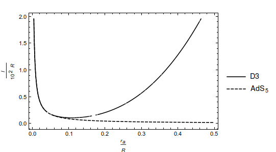
Figure 3: Width of the strip $l/R$ against $r_{a}/R$ for $r_{b}/R=10^{3}$ and $r_{a}/R<0.4$.

Actually this plots shows the comparison between the AdS limit and the D3-brane space, the agreement is conspicuous in the region where $r_{a}/R<0.1$, which is the minimum of the D3-brane plot. At this minimum the width of the strip is $l/R\approx 10.4$ for the D3-brane case. In this example we have chosen $r_{b}/R=10^{3}$ as the cut-off. See also Niarchos:2017cdz for a recent related discussion.

The next plot we present in fig.4 shows the comparison between the D3-brane case and the flat-space approximation for the width of the strip $l/R$ against $r_{a}/R$. In this case a cut-off of $r_{b}/R=10^{4}$ was used and we considered a region $r_{a}/R>10$. As we can see from this plot, the agreement between both backgrounds are satisfactory in that region.

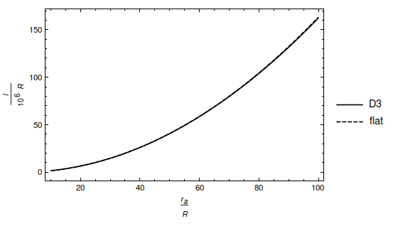
Figure 4: Width of the strip $l/R$ against $r_{a}/R$ for $r_{b}/R=10^{4}$ and $r_{a}/R>10$.

In the next plot of fig.5 this time we present the dimensionless entanglement entropy $s$ against $l/R$. Actually a comparison between the plots for the D3-brane and AdS backgrounds are shown. This was made for the cut-off of $r_{b}/R=10^{3}$ in the region $r_{a}/R<0.4$. From this plot we can see that for the D3-brane background the entanglement entropy $s$ has two branches. The superior branch corresponds to the region $r_{a}/R<0.1$ and the inferior one to region $r_{a}/R>0.1$. Note that the superior branch coincides with the AdS case.

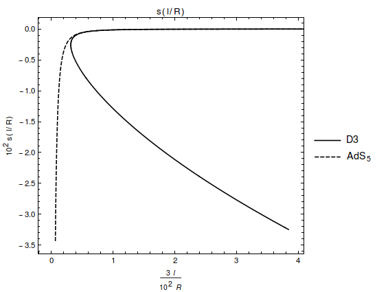
Figure 5: Entanglement entropy $s$ against $l/R$ for $r_{b}/R=10^{3}$ and $r_{a}/R<0.4$.

In the next plot of fig.6 we present a comparison between the entanglement entropy of the D3-brane and flat-space backgrounds. In this plot we consider the cut-off of $r_{b}/R=10^{4}$ and the region $r_{a}/R>10$. We see from this figure that the plot of both backgrounds have a satisfactory agreement in that region.

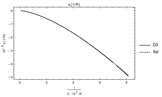
Figure 6: Entanglement entropy $s$ against for $r_{b}/R=10^{4}$ and $r_{a}/R>10$.

3 Entanglement entropy for the M2-brane background

In this section we do the computation of entanglement entropy ($S_{A}$) corresponding to the 11-dimensional supergravity M2-brane background. The metric solution generated by N coincident M2-branes is Review2 :

$$ds^{2}_{\text{M2}}=dx^{\mu}dx^{\nu}g_{\mu\nu}=\left(1+\frac{R_{2}^{6}}{r^{6}}\right)^{-2/3}(-dt^{2}+dx_{2}^{2})+\left(1+\frac{R_{2}^{6}}{r^{6}}\right)^{1/3}(dr^{2}+r^{2}d\Omega^{2}_{7}),$$ (22)

where $x^{\mu}=(t,x^{a},r,\theta_{b})$, with $a=1,2$ and $b=1,2...7$, are the space-time coordinates, $g_{\mu\nu}$ is the space-time metric, $R_{2}=(32\pi Nl^{6}_{11})^{1/6}$, $l_{11}$ is the Plank’s length in eleven dimensions, $dx_{2}^{2}$ is the euclidean line element in $\mathbb{R}^{2}$ and $d\Omega^{2}_{7}$ is the line element on the 7-sphere which only depends on $\theta_{b}$ coordinates.

3.1 Rectangular strip

As we worked in the last section, we take a 2-dimensional ($d=2$) subsystem $A\in\mathbb{R}^{2}$ as the following rectangular strip:

$$X=x^{1}\in\left[-\frac{l}{2},\frac{l}{2}\right]\,\,\,\,,\,\,\,\,\,x^{2}\in\left[-\frac{L}{2},\frac{L}{2}\right]$$ (23)

Now we parametrize the $\gamma$-surface as follows: $x^{1}=X(r)$, $\sigma_{1}=r$ and $\sigma_{2}=x^{2}$. The rest of the coordinates are independent of this parametrization. Then the area of this surface is given by:

$$\mathcal{A}=\int d^{2}\sigma\sqrt{det(G_{\alpha\beta})},$$ (24)

where $G_{\alpha\beta}=\partial_{\alpha}x^{\mu}\partial_{\beta}x^{\nu}g_{\mu\nu}$ is the induced metric on the $\gamma$-surface.

After the computation of this area $\mathcal{A}$ in the M2-brane background we obtain:

$$\mathcal{A}=L\int dr\sqrt{\frac{X^{\prime 2}}{f^{4}(r)}+\frac{1}{f(r)}}$$ (25)

where $f(r)=\left(1+\frac{R^{6}_{2}}{r^{6}}\right)^{1/3}$.

From this area functional we can derive the equation for the profile $X(r)$ of the surface that extremize this area, this equation is given by:

$$\frac{dX}{dr}=\pm\sqrt{\frac{f^{7}(r)}{f^{4}(r_{a})-f^{4}(r)}}.$$ (26)

As in the previous section $r_{a}$ represents the closest approach of the profile $X(r)$ to the origin of coordinates. This profile has two branches that join smoothly at $r_{a}$, where $X=0$ and $X^{\prime}\rightarrow\infty$. We also take $r_{b}$ as the UV cut-off in such a way that the width of the strip $l$ is given by:

$$X(r_{b})=\pm\frac{l}{2}.$$ (27)

If we solve the eq.(26) with the boundary condition (27) we obtain the width of the strip as an integral expression that depends on $r_{a}$ and $r_{b}$.

$$\frac{l}{2}=\int_{r_{a}}^{r_{b}}dr\sqrt{\frac{f^{7}(r)}{f^{4}(r_{a})-f^{4}(r)}}.$$ (28)

As was pointed out in the previous section $r_{a}$ could be determined by inverting eq.(28). The result would be in terms of $l$ and $r_{b}$. After substitution of the equation for the extremal surface (26) into the functional area (25) and taking the limits of integration used in eq.(28) we finally obtain the extremal area:

$$\mathcal{A}=L\int_{r_{a}}^{r_{b}}dr\sqrt{\frac{f^{4}(r_{a})}{f(r)[f^{4}(r_{a})-f^{4}(r)]}}.$$ (29)

As we can observe $f(r)$ is a monotonic decreasing function with maximum $f(r_{a})$ and minimum $f(\infty)\rightarrow 1$. Then the integrand of eq.(29) goes to a constant as $r\rightarrow\infty$. Hence we have that the area $\mathcal{A}$ is divergent as $r_{b}\rightarrow\infty$. The divergent part of the area $\mathcal{A}$ can be defined in terms of UV cut-off $r_{b}$ as:

$$\mathcal{A}_{\text{div}}=L\int_{0}^{r_{b}}dr\sqrt{\frac{f^{4}(r_{a})}{f(r)[f^{4}(r_{a})-1]}}.$$ (30)

The entanglement entropy can be computed from area $\mathcal{A}$ and RT-formula (1). We may write schematically this entropy as follows:

$$S_{A}=S_{\text{div}}+\frac{LR_{2}}{4G_{N}^{4}}\,\,s\left(\frac{l}{R_{2}}\right),$$ (31)

where $S_{\text{div}}$ is the divergent part of the entropy and $s(l/R_{2})$ is a dimensionless finite part of the entanglement entropy as a function of $l/R_{2}$. Not always it is possible to put this dimensionless entropy as a explicitly function of $l/R_{2}$. In general what we can only do is to put this dimensionless entropy in terms of $r_{a}$ and $r_{b}$:

$$s(r_{a})=\int_{r_{a}}^{r_{b}}\frac{dr}{R_{2}}\sqrt{\frac{f^{4}(r_{a})}{f(r)[f^{4}(r_{a})-f^{4}(r)]}}-\int_{0}^{r_{b}}\frac{dr}{R_{2}}\sqrt{\frac{f^{4}(r_{a})}{f(r)[f^{4}(r_{a})-1]}}.$$ (32)

3.2 Near horizon limit: $AdS_{4}\times S^{7}$

This limit geometry of the N M2-branes are obtained when we take $R_{2}>>r$ so that $f\approx\frac{R^{2}_{2}}{r^{2}}$. In this case the dual theory corresponds to the ABMJ theory in $D=3$ Aharony:2008ug . Then if we compute the width of the strip (28) in this background limit we obtain:

$$\frac{l}{R_{2}}=\frac{2R_{2}^{2}}{r_{a}^{2}}\int_{1}^{\frac{r_{b}}{r_{a}}}\frac{dx}{x^{3}\sqrt{x^{8}-1}}=\frac{R_{2}^{2}}{r_{a}^{2}}c_{2}\left[1+\mathcal{O}\left(\frac{r_{a}^{6}}{r_{b}^{6}}\right)\right],$$ (33)

where $c_{2}=\frac{\sqrt{\pi}\Gamma(3/4)}{\Gamma(1/4)}$. In what follows we are going to disregard the superior order $\mathcal{O}\left(\frac{r_{a}^{6}}{r_{b}^{6}}\right)$ in this result.

The entanglement entropy in this limit background can be calculated from the extremal area $\mathcal{A}$ (eq.29) and the RT-formula (eq.1), as a result we obtain:

$$S_{A}=\frac{Lr_{a}^{2}}{4RG_{N}^{4}}\int_{1}^{r_{b}/r_{a}}dx\frac{x^{5}}{\sqrt{x^{8}-1}}=\frac{Lr_{b}^{2}}{4G_{N}^{4}r_{a}}-\frac{Lc_{2}r_{a}^{2}}{8G_{N}^{4}R_{2}}.$$ (34)

Notice that the first term of this expression is divergent as $r_{b}\rightarrow\infty$. This term can be also be obtained directly from eq.(30).

Now we eliminate the parameter $r_{a}$ from these last two equations in order to put the entanglement entropy $S_{A}$ as a function of the width of strip $l$:

$$S_{A}=\frac{Lr_{b}^{2}}{4G_{N}^{4}R_{2}}-\frac{Lc_{2}^{2}R_{2}^{2}}{8G_{N}^{4}l}.$$ (35)

Up to an arbitrary constant factor in the divergent part of this equation, this result agrees with the one obtained in Ryu:2006bv . Then in this regime the dimensionless finite entanglement entropy results:

$$s(l/R_{2})=-\frac{c_{2}^{2}R_{2}}{2l}.$$ (36)

3.3 Flat-space limit

This background of an almost flat space is obtained as a result of assuming that $R_{2}<<r$. This implies that $f\approx 1+\frac{R_{2}^{6}}{3r^{6}}$. This case corresponds, in the field theory side, to a non-conformal nor supersymmetric gauge theory $SU(N)$ in $D=3$. Then we can calculate the width of the strip (eq.28):

$$\frac{l}{R_{2}}\approx\frac{\sqrt{3}r_{a}^{4}}{R_{2}^{4}}\int_{1}^{\frac{r_{b}}{r_{a}}}dx\frac{x^{3}}{\sqrt{x^{6}-1}}\approx\sqrt{3}\left(\frac{r_{a}}{R_{2}}\right)^{3}\frac{r_{b}}{R_{2}}.$$ (37)

Also in this background limit we can calculate the entanglement entropy starting from eq.(29) and applying the RT-formula (eq.1):

$$S_{A}\approx\frac{\sqrt{3}L}{8G_{N}^{4}R_{2}^{3}}r_{a}^{4}\int_{1}^{\frac{r_{b}}{r_{a}}}dx\frac{x^{3}}{\sqrt{x^{6}-1}}=\frac{\sqrt{3}Lr_{a}^{3}r_{b}}{48G_{N}^{4}R_{2}^{3}}-\frac{\sqrt{3}Lr_{a}^{4}c^{\prime}}{8G_{N}^{4}R_{2}^{3}},$$ (38)

where $c^{\prime}=\frac{\sqrt{\pi}\Gamma(5/6)}{\Gamma(1/3)}$. The first term of this expression diverges as $r_{b}\rightarrow\infty$. This divergent term can also be obtained directly from eq.(30).

Now we eliminate the parameter $r_{a}$ from these last two expressions in order to have the entanglement entropy $S_{A}$ as a function of the width of the strip $l$:

$$S_{A}=\frac{Ll}{48G_{N}^{4}}-\frac{Lc^{\prime}R_{2}}{8(3)^{1/6}G_{N}^{4}}\left(\frac{l}{r_{b}}\right)^{4/3},$$ (39)

As we can see the first term of this equation is proportional to $l$. This term corresponds to the divergent part of $S_{A}$. This is because from eq.(37) the width of the strip $l\sim r_{b}$. Then the dimensionless entanglement entropy is:

$$s(l/R_{2})=-\frac{c^{\prime}}{2(3)^{1/6}}\left(\frac{l}{r_{b}}\right)^{4/3},$$ (40)

This novel result still contains the UV cut-off $r_{b}$, however, it continues to be a finite function. This is so because according to eq.(37) $l/R_{2}$ is finite and can be expressed in terms of $r_{a}$.

3.4 M2-brane and asymptotic limits

In the case of the M2-brane background we can do a numerically study of the behaviour of the entanglement entropy. Let’s start by plotting (see fig.7) a comparison between the width of the strip $l/R_{2}$ for the general M2-brane space (eq.28) and for the AdS₄ limit (eq.33). This was done with the cut-off of $r_{b}/R_{2}=10^{2}$ and for the region $r_{a}/R_{2}<2$. As we can see from this figure both plots coincide for the region $r_{a}/R<0.32$, which is where the plot for the M2-brane has its minimum, which is $l/R_{2}=8.32$ .

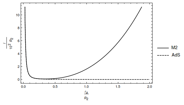
Figure 7: $l/R_{2}$ against $r_{a}/R_{2}$ for $r_{b}/R_{2}=10^{2}$.

Next we plot (see fig.8) a comparison between the width of the strip for the M2-brane (eq.28) and the almost-flat space limit (eq.37). This plot was done considering $r_{b}/R_{2}=10^{3}$ and the region $r_{a}/R_{2}>5$. As we can see from this picture the coincidence is very good in such region.

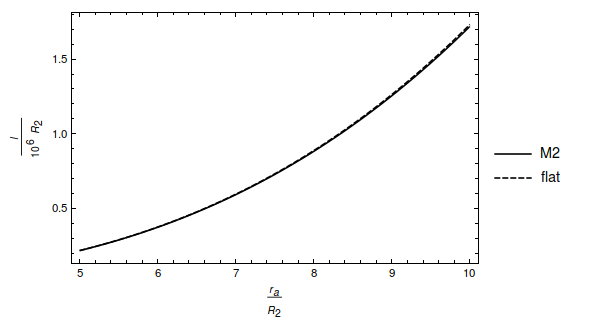
Figure 8: $l/R_{2}$ against $r_{a}/R_{2}$ for $r_{b}/R_{2}=10^{3}$.

Now is time to analyse the dimensionless entanglement entropy $s(l/R_{2})$. So first we plot (see fig.9) a comparison between the entanglement entropy for the general M2-brane space (eq.31) and for the AdS₄ space limit (eq.36). This plot was done considering the UV cut-off $r_{b}/R_{2}=10^{2}$ and the region $r_{a}/R_{2}<1$. As we can see from this figure there are two branches for the M2-brane background, the superior one corresponds to $r_{a}/R_{2}<0.32$ and the inferior one $r_{a}/R_{2}>0.32$. The coincidence of the plots occurs in the superior branch of the M2-brane entropy plot.

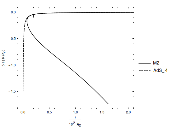
Figure 9: $s(l/R_{2})$ against $l/R_{2}$ for $r_{b}/R_{2}=10^{2}$.

Next we plot (see fig.10) a comparison between the dimensionless entanglement entropy for the general M2-brane background (eq.31) and for the almost-flat space limit ( eq.40). In this case we used a UV cut-off $r_{b}/R_{2}=10^{3}$ and consider the region $r_{a}/R_{2}>5$. As we can see from this figure, both plots coincide very well in such region.

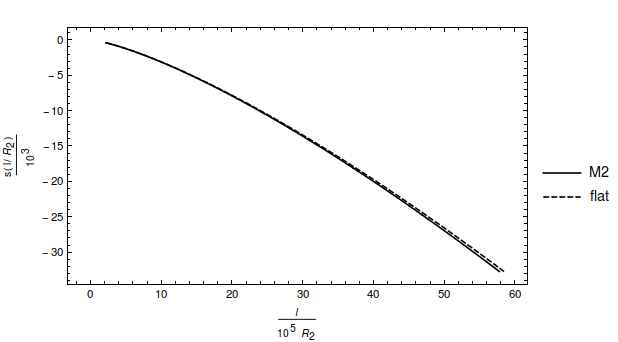
Figure 10: Entanglement entropy $s(l/R_{2})$ for $r_{b}/R_{2}=10^{3}$.

4 Entanglement entropy for the M5-brane background

In this section we compute the entanglement entropy ($S_{\mathcal{A}}$) corresponding to the background space-time generated by N coincident M5-branes. The 11-dimensional supergravity solution of M5-branes is given by the metric Review2 ; Review1 :

$$ds^{2}_{\text{M5}}=g_{\mu\nu}dx^{\mu}dx^{\nu}=\left(1+\frac{R_{5}^{3}}{r^{3}}\right)^{-1/3}dx_{6}^{2}+\left(1+\frac{R_{5}^{3}}{r^{3}}\right)^{2/3}(dr^{2}+r^{2}d\Omega^{2}_{4}),$$ (41)

where $x^{\mu}=(t,x^{a},r,\theta_{b})$, with $a=1,2,...5$ and $b=1,2...4$, are the space-time coordinates, $g_{\mu\nu}$ is the space-time metric, $R_{5}=(\pi Nl_{11}^{3})^{1/3}$ , $l_{11}$ is the Plank’s length in eleven dimensions, $dx_{5}^{2}$ is the euclidean line element in $\mathbb{R}^{5}$ and $d\Omega^{2}_{4}$ is the line element on the 4-sphere which only depends on $\theta_{b}$ coordinates.

4.1 Rectangular strip

In order to compute the entanglement entropy we consider a subsystem $A\in\mathbb{R}^{5}$ ($d=5$) as the following strip:

$$X\equiv x^{1}=\left[-\frac{l}{2},\frac{l}{2}\right]\,\,\,\,\,,\,\,\,\,\,\,x^{2,3,4,5}=\left[-\frac{L}{2},\frac{L}{2}\right]$$ (42)

Now we parametrize the $\gamma$-surface as: $x^{1}=X(r)$, $r=\sigma^{1}$, $x^{i}=\sigma^{i}$ with $i=2,..5$. The rest of the coordinates are independent of this prametrization. As we did in the previous sections we can compute the area of the $\gamma$-surface in this parametrization following the next formula:

$$\mathcal{A}=\int d^{5}\sigma\sqrt{det(G_{\alpha\beta})},$$ (43)

where $G_{\alpha\beta}=\partial x^{\mu}\partial x^{\nu}g_{\mu\nu}$ is the induced metric on the $\gamma$-surface. Then the area $\mathcal{A}$ turns out to be a functional of the surface profile $X(r)$ and can be written down as follows:

$$\mathcal{A}=L^{4}\int dr\sqrt{\frac{X^{\prime 2}}{f^{5}}+\frac{1}{f^{2}}},$$ (44)

where $f=\left(1+\frac{R^{3}_{5}}{r^{3}}\right)^{1/3}$ and $X^{\prime}\equiv dX/dr$. From this functional $\mathcal{A}$ we can derive the equation for the profile $X(r)$ that extremize the area of the surface. Such equation can be written down as follows:

$$\frac{dX}{dr}=\pm\frac{f^{4}(r)}{\sqrt{f^{5}(r_{a})-f^{5}(r)}},$$ (45)

where as in the previous sections $r_{a}$ is the closest point to the origin of coordinates, besides $X(r_{a})=0$ and $X^{\prime}(r_{a})\rightarrow\infty$. We also need to define a UV cut-off which we call $r_{b}$ and that satisfy the following boundary condition:

$$X(r_{b})=\pm\frac{l}{2}.$$ (46)

Now we can compute the width of the strip $l$ in terms of the parameter $r_{a}$ and $r_{b}$. To do so we integrate eq.(45) subject to the above boundary condition. Then the result is as follows:

$$\frac{l}{2}=\int_{r_{a}}^{r_{b}}dr\frac{f^{4}(r)}{\sqrt{f^{5}(r_{a})-f^{5}(r)}}.$$ (47)

Note that we could obtain the parameter $r_{a}$ after inverting this equation. The result would be in terms of $l$ and $r_{b}$.

Now we will find the entanglement entropy $S_{A}$. In order to do so first we are going to find the extreme area $\mathcal{A}$ which follows from substituting the eq.(45) into the functional area (eq.44). The result is the next extremal area:

$$\mathcal{A}=L^{4}\int_{r_{a}}^{r_{b}}dr\frac{1}{f(r)}\sqrt{\frac{f^{5}(r_{a})}{f^{5}(r_{a})-f^{5}(r)}}.$$ (48)

Since $f(r)$ is a monotonic decreasing function that has maximum $f(r_{a})$ and minimum $f(\infty)=1$, we have that the integrand of this expression goes to a constant factor as $r\rightarrow\infty$. As a result we can conclude that this integral diverges as $r_{b}\rightarrow\infty$. In order to have a finite result for the entanglement entropy we must separate the divergent part from this expression as follows:

$$\mathcal{A}=\mathcal{A}_{\text{div}}+\mathcal{A}_{\text{fin}},$$ (49)

where the divergent part of this area can be defined in terms of the UV cut-off $r_{b}$ as:

$$\mathcal{A}_{\text{div}}=L^{4}\int_{0}^{r_{b}}dr\frac{1}{f(r)}\sqrt{\frac{f^{5}(r_{a})}{f^{5}(r_{a})-1}}.$$ (50)

From the equation for the area $\mathcal{A}$ (eq.49) and from the RT-formula (eq.1) we can schematically write down the entanglement entropy as follows:

$$S=S_{\text{div}}+\frac{L^{4}R_{5}}{4G_{N}^{7}}\,\,s\left(\frac{l}{R_{5}}\right),$$ (51)

where the dimensionless function $s(l/R_{5})$ is the finite part of the entanglement entropy. It is not always possible to express this dimensionless entropy $s$ as a function of $l$, however we can put this entropy in terms of $r_{a}$ and $r_{b}$ which follows from eqs.(48) and (50):

$$s(r_{a})=\int_{r_{a}}^{r_{b}}\frac{dr}{R_{2}}\frac{1}{f(r)}\sqrt{\frac{f^{5}(r_{a})}{f^{5}(r_{a})-f^{5}(r)}}-\int_{0}^{r_{b}}\frac{dr}{R_{2}}\frac{1}{f(r)}\sqrt{\frac{f^{5}(r_{a})}{f^{5}(r_{a})-1}}.$$ (52)

4.2 Near horizon limit: $AdS_{7}\times S^{4}$

This limit geometry of the N M5-branes are obtained if we take the approximation $R_{5}>>r$ which implies that $f\approx\frac{R_{5}}{r}$. In this case the dual theory is the $D=6$ superconformal field theory. So if calculate the width of the strip $l$ (eq.47) in this limit we will obtain:

$$\frac{l}{R_{5}}=\frac{2R_{5}^{1/2}}{r_{a}^{1/2}}\int_{1}^{\frac{r_{b}}{r_{a}}}dx\frac{1}{\sqrt{x^{3}(x^{5}-1)}}=\frac{4R_{5}^{1/2}c_{5}}{r_{a}^{1/2}}\left[1+\mathcal{O}\left(\frac{r_{a}^{3}}{r_{b}^{3}}\right)\right],$$ (53)

where $c_{5}=\frac{\sqrt{\pi}\Gamma(3/5)}{\Gamma(1/10)}$. In what follows we are going to disregard the superior order $\mathcal{O}\left(\frac{r_{a}^{3}}{r_{b}^{3}}\right)$ in our calculations.

Next we compute the entanglement entropy in this background limit. This follows from the equation for the area $\mathcal{A}$ (eq.48) and from the RT-formula (eq.1):

$$S_{A}=\frac{L^{4}r_{a}^{2}}{4G_{N}^{7}R_{5}}\int_{1}^{\frac{r_{b}}{r_{a}}}dx\sqrt{\frac{x^{7}}{x^{5}-1}}=\frac{L^{4}r_{b}^{2}}{20G_{N}^{7}R_{5}}-\frac{c_{5}L^{4}r_{a}^{2}}{8G_{N}^{7}R_{5}}.$$ (54)

Notice that the first term of this expression contains the UV cut-off $r_{b}$ and that this term diverges as $r_{b}\rightarrow\infty$. This divergent term can be also be obtained from eq.(50).

Now in order to find the entanglement entropy $S_{A}$ in terms of the width of the strip $l$, we eliminate the parameter $r_{a}$ from the last two equations, as a result we find:

$$S_{A}=\frac{L^{4}r_{b}^{2}}{20G_{N}^{7}R_{5}}-\frac{32L^{4}c_{5}^{5}R_{5}^{5}}{G_{N}^{7}l^{4}}.$$ (55)

This result agrees with the one found in Ryu:2006bv . Then the dimensionless finite entanglement entropy is in this case:

$$s(l/R_{5})=-\frac{128c_{5}^{5}R_{5}^{4}}{l^{4}}.$$ (56)

4.3 Flat-space limit

In this case, we will find the entanglement entropy in the approximate almost-flat space geometry which results from taking the limit $R_{5}<<r$ in our computations. In this limit, we have that $f\approx 1+\frac{R_{5}^{3}}{3r^{3}}$. In this asymptotic limit, the dual field theory (when it exist) is a non-conformal nor supersymmetric $D=6$ theory with $SU(N)$ gauge group. Then if we calculate the width of the strip (eq.47) in this background limit we will obtain:

$$\frac{l}{R_{5}}\approx\frac{2\sqrt{3/5}r_{a}^{5/2}}{R_{5}^{5/2}}\int_{1}^{\frac{r_{b}}{r_{a}}}dx\sqrt{\frac{x^{3}}{x^{3}-1}}\approx 2\sqrt{3/5}\left(\frac{r_{a}}{R_{5}}\right)^{3/2}\frac{r_{b}}{R_{5}}.$$ (57)

Then the entanglement entropy in this background limit follows from eq.(48) and from the RT-formula (eq.1):

$$S_{A}\approx\frac{\sqrt{3/5}L^{4}r_{a}^{5/2}}{4G_{N}^{7}R_{5}^{3/2}}\int_{1}^{\frac{r_{b}}{r_{a}}}dx\sqrt{\frac{x^{3}}{x^{3}-1}}=\frac{\sqrt{3/5}L^{4}r_{a}^{3/2}r_{b}}{12G_{N}^{7}R_{5}^{3/2}}-\frac{\sqrt{3/5}c_{5}^{*}L^{4}r_{a}^{5/2}}{4G_{N}^{7}R_{5}^{3/2}},$$ (58)

where $c_{5}^{*}=\frac{\sqrt{\pi}\Gamma(2/3)}{\Gamma(1/6)}$. Note that the first term of this expression correspond to the divergent part of the entropy. This is because this term diverges as the UV cut-off $r_{b}\rightarrow\infty$. Also the divergent part of this entropy can be obtained from eq.(50).

In order to have the entanglement entropy $S_{A}$ in terms of the width of the strip $l$, we eliminate the parameter $r_{a}$ from these last couple of equations, as a result we find:

$$S_{A}=\frac{L^{4}l}{24G_{N}^{7}}-\frac{c_{5}^{*}L^{4}R_{5}}{2^{11/3}(3/5)^{1/3}G_{N}^{7}}\left(\frac{l}{r_{b}}\right)^{5/3}.$$ (59)

Then the dimensionless finite entanglement entropy is:

$$s(l/R_{5})=-\frac{c_{5}^{*}}{2^{5/3}(3/5)^{1/3}}\left(\frac{l}{r_{b}}\right)^{5/3}.$$ (60)

This novel result stills contains the UV cut-off $r_{b}$, however, it continues to be a finite function since the ratio $\frac{l}{r_{b}}$ is finite according to (57).

4.4 M5-brane and asymptotic limits

In the M5-brane background, we can analyse numerically the entanglement entropy and compare this with its limit geometric background cases. So first we plot (see fig.11) a comparison between the width of the strip $l/R_{5}$ for the cases of M2-brane and AdS₇. We can observe from this plot that the minimum of $l/R_{5}$ ($l/R_{5}=6.08$) for the M5-brane case is reached at $r_{a}/R_{5}=0.048$. These plots were made at $r_{b}/R_{5}=10^{3}$ and for the region $r_{a}/R_{5}<0.2$.

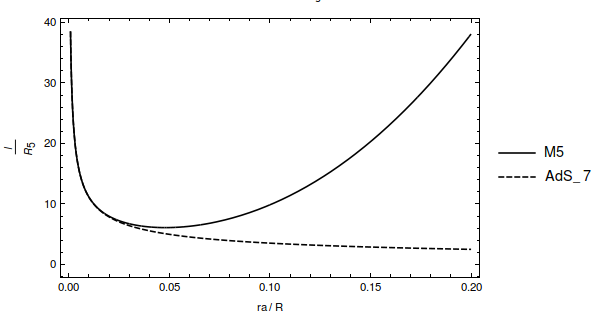
Figure 11: $l/R_{5}$ agaisnt $r_{a}/R_{5}$ for $r_{a}/R_{5}<0.2$ $r_{b}/R_{5}=10^{3}$.

Next we plot (see fig.12) a comparison between the dimensionless entropy $s(l/R_{5})$ against $l/R_{5}$ for M5-brane and AdS₇ backgrounds cases. As we can see from this figure the dimensionless entropy for the M5-brane has two branches, the superior one corresponds to $r_{a}/R_{5}<0.048$ and the inferior one corresponds to $r_{a}/R_{5}>0.048$. As we can notice the superior brach coincides very well with the AdS₇ plot at the regime $r_{a}/R_{5}<0.048$.

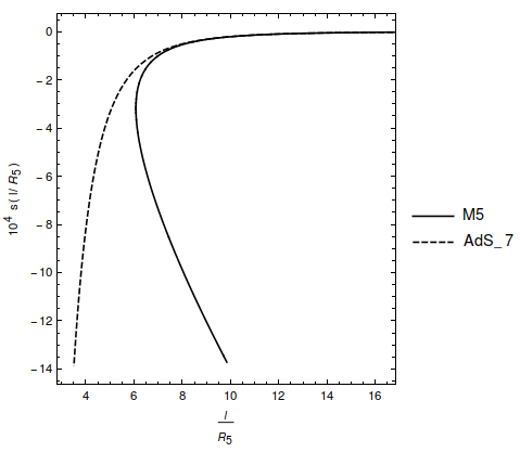
Figure 12: Entanglement entropy $s(l/R_{5})$ for $r_{b}/R_{5}=10^{3}$.

Now we plot (see fig.13) the comparison between the dimensionless entropy $s(l/R_{5})$ for the M5-brane and almost-flat backgrounds cases. These plots were made in the regime $r_{a}/R_{5}>4$ and for the UV cut-off $r_{b}/R_{5}=5\times 10^{3}$. As we can see from the figure the plots coincide very well in such regime.

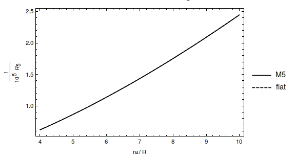
Figure 13: $l/R_{5}$ against $r_{a}/R_{5}$ for $r_{a}/R_{5}>4$ and $r_{b}/R_{5}=5\times 10^{3}$.

Next we plot (see fig.14) a comparison between the dimensionless entropy $s(l/R_{5})$ against $l/R_{5}$ for the M5-brane and almost-flat backgrounds cases. These plot were made for the interval $r_{a}/R_{5}>4$ and for the UV cut-off of $r_{b}/R_{5}=5\times 10^{3}$. As we can see these plots coincide very well in such a regime.

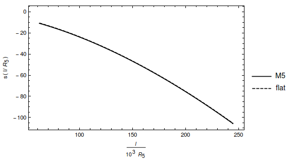
Figure 14: Entanglement entropy $s(l/R_{5})$ for $r_{a}/R_{5}>4$ and $r_{b}/R_{5}=5\times 10^{3}$.

5 Conclusions

In this paper, in the context of Gauge/Gravity dualities, we have investigated some aspects of quantum entanglement in large N gauge theories that are dual to strings/M-theory in D3, M2-, M5-brane background spaces. Mainly, we have computed the quantum entanglement entropy of those theories applying the RT-formula for D3-, M2-, and M5-brane background spaces. This is done analytically for the asymptotic limit cases: AdS geometries, which results agree with the literature, and the almost flat-space geometries, that are novel results. Numerically, we have obtained entanglement entropies for the D3-, M2-, and M5-brane spaces and have compared them with their asymptotic geometric limis. The entanglement entropies for these branes do not have in general a single valued behaviour, instead all of these entropies have two branches, one going asymptotically (as the ratio $r_{a}/R$ decrease) to the AdS behaviour and the other (as the $r_{a}/R$ increase) to the flat-space limits.

We have also noticed that the choice of the UV cut-off value plays a crucial role in the behaviour of the entanglement entropy function. For a big enough cut-off value, the entanglement entropy function tends to have a decreasing behaviour in all the backgrounds that we have studied.

It will be interesting to investigate the non-conformal dual theories that we mention in this work and also the entanglement entropy for the case of non-extremal branes. In ref. Niarchos:2017cdz , it has been suggested that the D3-brane case could be related to the open-closed string duality. This may offer a possible interpretation for the M2- and M5- cases.

- (1) J. D. Bekenstein, “Black holes and entropy,” Phys. Rev. D 7, 2333 (1973).
- (2) S. W. Hawking, “Black Holes and Thermodynamics,” Phys. Rev. D 13, 191 (1976).
- (3) A. Strominger and C. Vafa, “Microscopic origin of the Bekenstein-Hawking entropy,” Phys. Lett. B 379, 99 (1996) [hep-th/9601029].
- (4) S. S. Gubser, I. R. Klebanov and A. W. Peet, “Entropy and temperature of black 3-branes,” Phys. Rev. D 54, 3915 (1996) [hep-th/9602135].
- (5) J. M. Maldacena, “The Large N limit of superconformal field theories and supergravity,” Int. J. Theor. Phys. 38, 1113 (1999) [Adv. Theor. Math. Phys. 2, 231 (1998)] [hep-th/9711200].
- (6) S. Hawking, J. M. Maldacena and A. Strominger, “de Sitter entropy, quantum entanglement and AdS / CFT,” JHEP 0105, 001 (2001) [hep-th/0002145].
- (7) S. Ryu and T. Takayanagi, “Holographic derivation of entanglement entropy from AdS/CFT,” Phys. Rev. Lett. 96, 181602 (2006) [hep-th/0603001].
- (8) S. Ryu and T. Takayanagi, “Aspects of Holographic Entanglement Entropy,” JHEP 0608, 045 (2006) [hep-th/0605073].
- (9) V. E. Hubeny, M. Rangamani and T. Takayanagi, “A Covariant holographic entanglement entropy proposal,” JHEP 0707, 062 (2007) [arXiv:0705.0016 [hep-th]].
- (10) I. Bah, A. Faraggi, L. A. Pando Zayas and C. A. Terrero-Escalante, “Holographic entanglement entropy and phase transitions at finite temperature,” Int. J. Mod. Phys. A 24, 2703 (2009) [arXiv:0710.5483 [hep-th]].
- (11) M. Fujita, T. Nishioka and T. Takayanagi, “Geometric Entropy and Hagedorn/Deconfinement Transition,” JHEP 0809, 016 (2008) [arXiv:0806.3118 [hep-th]].
- (12) T. Nishioka, S. Ryu and T. Takayanagi, “Holographic Entanglement Entropy: An Overview,” J. Phys. A 42, 504008 (2009) [arXiv:0905.0932 [hep-th]].
- (13) J. Maldacena and G. L. Pimentel, “Entanglement entropy in de Sitter space,” JHEP 1302, 038 (2013) [arXiv:1210.7244 [hep-th]].
- (14) Y. Bea, J. D. Edelstein, G. Itsios, K. S. Kooner, C. Nunez, D. Schofield and J. A. Sierra-Garcia, “Compactifications of the Klebanov-Witten CFT and new AdS3 backgrounds,” JHEP 1505, 062 (2015) [arXiv:1503.07527 [hep-th]].
- (15) C. Cao, S. M. Carroll and S. Michalakis, “Space from Hilbert Space: Recovering Geometry from Bulk Entanglement,” Phys. Rev. D 95, no. 2, 024031 (2017) [arXiv:1606.08444 [hep-th]].
- (16) R. Mishra and H. Singh, “Perturbative entanglement thermodynamics for AdS spacetime: Renormalization,” JHEP 1510, 129 (2015) [arXiv:1507.03836 [hep-th]].
- (17) R. Mishra and H. Singh, “Entanglement asymmetry for boosted black branes and the bound,” Int. J. Mod. Phys. A 32, no. 16, 1750091 (2017) [arXiv:1603.06058 [hep-th]].
- (18) A. Ghosh and R. Mishra, “An Inhomogeneous Jacobi equation for minimal surfaces and perturbative change of Holographic Entanglement Entropy,” arXiv:1710.02088 [hep-th].
- (19) V. Niarchos, “Holographic entanglement entropy in open-closed string duality,” arXiv:1701.03113 [hep-th].
- (20) G. T. Horowitz and A. Strominger, “Black strings and P-branes,” Nucl. Phys. B 360 (1991) 197.
- (21) S. S. Gubser, I. R. Klebanov and A. M. Polyakov, “Gauge theory correlators from noncritical string theory,” Phys. Lett. B 428 (1998) 105 [hep-th/9802109].
- (22) W. Fischler, A. Kundu and S. Kundu, JHEP 1401, 137 (2014) doi:10.1007/JHEP01(2014)137 [arXiv:1307.2932 [hep-th]].
- (23) S. S. Gubser, I. R. Klebanov and A. M. Polyakov, “Gauge theory correlators from noncritical string theory,” Phys. Lett. B 428, 105 (1998) [hep-th/9802109].
- (24) E. Witten, “Anti-de Sitter space and holography,” Adv. Theor. Math. Phys. 2, 253 (1998) [hep-th/9802150].
- (25) O. Aharony, S. S. Gubser, J. M. Maldacena, H. Ooguri and Y. Oz, “Large N field theories, string theory and gravity,” Phys. Rept. 323, 183 (2000) [hep-th/9905111].
- (26) J. L. Petersen, “Introduction to the Maldacena conjecture on AdS / CFT,” Int. J. Mod. Phys. A 14, 3597 (1999) [hep-th/9902131].
- (27) O. Aharony, O. Bergman, D. L. Jafferis and J. Maldacena, “N=6 superconformal Chern-Simons-matter theories, M2-branes and their gravity duals,” JHEP 0810, 091 (2008) [arXiv:0806.1218 [hep-th]].