Reconstruction of a direction-dependent primordial power spectrum from Planck CMB data

Amel Durakovic    Paul Hunt    Suvodip Mukherjee    Subir Sarkar    Tarun Souradeep
Abstract

We consider the possibility that the primordial curvature perturbation is direction-dependent. To first order this is parameterised by a quadrupolar modulation of the power spectrum and results in statistical anisotropy of the CMB, which can be quantified using ‘bipolar spherical harmonics’. We compute these for the Planck DR2–2015 SMICA map and estimate the noise covariance from Planck Full Focal Plane 9 simulations. A constant quadrupolar modulation is detected with 2.2σ2.2𝜎2.2\sigma significance, dropping to 2σ2𝜎2\sigma when the primordial power is assumed to scale with wave number k𝑘k as a power law. Going beyond previous work we now allow the spectrum to have arbitrary scale-dependence. Our non-parametric reconstruction then suggests several spectral features, the most prominent at k0.006Mpc1similar-to𝑘0.006superscriptMpc1k\sim 0.006~{}\mathrm{Mpc}^{-1}. When a constant quadrupolar modulation is fitted to data in the range 0.005k/Mpc10.0080.005𝑘superscriptMpc10.0080.005\leq k/\mathrm{Mpc}^{-1}\leq 0.008, its preferred directions are found to be related to the cosmic hemispherical asymmetry and the CMB dipole. To determine the significance we apply two test statistics to our reconstructions of the quadrupolar modulation from data, against reconstructions of realisations of noise only. With a test statistic sensitive only to the amplitude of the modulation, the reconstructions from the multipole range 30120030120030\leq\ell\leq 1200 are unusual with 2.1σ2.1𝜎2.1\sigma significance. With the second test statistic, sensitive also to the direction, the significance rises to 6.9σ6.9𝜎6.9\sigma. Our approach is easily generalised to include other data sets such as polarisation, large-scale structure and forthcoming 21-cm line observations which will enable these anomalies to be investigated further.

1 Introduction

The observed temperature fluctuations of the cosmic microwave background (CMB) radiation are believed to be due to curvature perturbations generated at an early stage in the evolution of the universe. The most discussed mechanism for this is the quantum fluctuations of a scalar field, the vacuum energy of which drives a period of accelerated expansion known as inflation. In the simplest scenario where the inflaton field evolves slowly down an almost flat potential, the (dimensionless) primordial power spectrum, which is the variance of the Fourier components of the curvature perturbation, is nearly scale-invariant, with slightly more power on large scales. Provided that the primordial power spectrum is independent of the direction (and the background cosmology is homogeneous and isotropic), the CMB fluctuations will also be statistically isotropic.

We consider here the possibility of a direction-dependent primordial power spectrum resulting in statistically anisotropic CMB fluctuations. In order for this to occur, some field must single out a particular direction uμsuperscript𝑢𝜇u^{\mu} and break rotational symmetry, and so the agent should either carry a space-time index or have a spatial gradient present in the initial field configuration. The first such model [1] considered a vector field Aμsuperscript𝐴𝜇A^{\mu} driving inflation via the effective scalar ξ=AμAμ𝜉subscript𝐴𝜇superscript𝐴𝜇\xi=A_{\mu}A^{\mu} with a sufficiently flat potential V(ξ)𝑉𝜉V(\xi). When the vector field singles out a direction, its energy-momentum tensor is no longer isotropic, so its direction-dependence can play a role gravitationally; in this case, inflation is followed by anisotropic expansion. Other work, motivated by some observational CMB anomalies, found that an anisotropy in the initial expansion rate following inflation can cause the fluctuations to inherit the anisotropy [2]. A concrete realisation of the anisotropy, with a vector field responsible, was subsequently proposed [3]. Such vector field models were, however, found to be unstable [4, 5]. It is important that the anisotropic field should not contribute significantly to the energy density, otherwise the expansion itself will be anisotropic to a degree in conflict with observations. Another possibility is that the vector field couples to the inflaton and thereby transfers the anisotropy, as in models with a coupling f(ϕ)2FμνFμν𝑓superscriptitalic-ϕ2subscript𝐹𝜇𝜈superscript𝐹𝜇𝜈f(\phi)^{2}F_{\mu\nu}F^{\mu\nu} where f(ϕ)𝑓italic-ϕf(\phi) is a function of the inflaton field and Fμν=μAννAμsubscript𝐹𝜇𝜈subscript𝜇subscript𝐴𝜈subscript𝜈subscript𝐴𝜇F_{\mu\nu}=\partial_{\mu}A_{\nu}-\partial_{\nu}A_{\mu} is the field strength of the vector field Aμsubscript𝐴𝜇A_{\mu} [6, 7].

All such models produce an angular modulation [8] such that the full (dimensionless) primordial power spectrum is:

𝒫(𝐤)𝒫𝐤\displaystyle\mathcal{P}(\mathbf{k}) =𝒫(k)+4πLMgLM(k)YLM(𝐤^).absent𝒫𝑘4𝜋subscript𝐿𝑀subscript𝑔𝐿𝑀𝑘subscript𝑌𝐿𝑀^𝐤\displaystyle=\mathcal{P}\left(k\right)+\sqrt{4\pi}\sum_{LM}g_{LM}(k)Y_{LM}(\mathbf{\hat{k}}). (1.1)

We adopt a data-driven approach, not committing to any specific theoretical model, and focus on the quadrupole modulation:

𝒫(𝐤)𝒫𝐤\displaystyle\mathcal{P}(\mathbf{k}) =𝒫(k)+4πM=22g2M(k)Y2M(𝐤^),absent𝒫𝑘4𝜋superscriptsubscript𝑀22subscript𝑔2𝑀𝑘subscript𝑌2𝑀^𝐤\displaystyle=\mathcal{P}\left(k\right)+\sqrt{4\pi}\sum_{M=-2}^{2}g_{2M}(k)Y_{2M}(\mathbf{\hat{k}}), (1.2)

where 𝒫(k)𝒫𝑘\mathcal{P}(k) is the usual isotropic power spectrum, Y2M(𝐤^)subscript𝑌2𝑀^𝐤Y_{2M}(\mathbf{\hat{k}}) are spherical harmonics that carry the direction-dependence and g2M(k)subscript𝑔2𝑀𝑘g_{2M}(k) are the associated harmonic space coefficients which may vary freely with the wave number k𝑘k and be either positive or negative. As the coefficients g2M(k)subscript𝑔2𝑀𝑘g_{2M}(k) determine the modulation, these are our main focus for reconstruction from data.

Note that we have chosen the split (1.2) in order to remain agnostic about the isotropic part of the primordial power spectrum, unlike the alternative parameterisation

𝒫(𝐤)𝒫𝐤\displaystyle\mathcal{P}(\mathbf{k}) =𝒫(k)(1+g(k)(𝐤^𝐧^)2),absent𝒫𝑘1𝑔𝑘superscript^𝐤^𝐧2\displaystyle=\mathcal{P}(k)(1+g(k)(\mathbf{\hat{k}}\cdot\mathbf{\hat{n}})^{2}), (1.3)

which reconstructs the shape of the quadrupole modulation relative to the isotropic primordial power spectrum. By contrast we reconstruct the absolute quadrupole modulation. Also, eq.(1.2) refers to the most general quadrupole modulation while the form of eq.(1.3) is a special case where the two directions that describe a general quadrupole coincide. Relations between g2Msubscript𝑔2𝑀g_{2M} and the two directions of a quadrupole are derived in Appendix A.

While g(k)𝑔𝑘g(k) is scale-invariant (up to logarithmic corrections) in most models, there is no fundamental reason for the quadrupole modulation to be scale-free. For example, in a study of perturbations in a Bianchi I universe which isotropises as inflation proceeds, g2M(k)subscript𝑔2𝑀𝑘g_{2M}(k) was found to have strong oscillatory features on large scales [9].111A limited duration of inflation was postulated so that the effects of the primordial anisotropic phase do not extend beyond the current horizon. Therefore we allow arbitrary scale-dependence of g2M(k)subscript𝑔2𝑀𝑘g_{2M}(k) and attempt to determine this from the data.

Symmetry considerations dictate that the quadrupole is the first modulation that can appear [8]. The next contribution would be the hexadecapole L=4𝐿4L=4 as only even L𝐿L are allowed (see § 2). Since the L=2𝐿2L=2 modulation is the first one that can appear and also has some theoretical motivation we will consider only this case although our formalism readily allows for the inclusion of higher order modulations.

The quadrupole modulation of the primordial power spectrum will manifest itself in the CMB temperature fluctuations which will now be statistically anisotropic. The temperature fluctuations ΔTΔ𝑇\Delta T are conventionally expanded in spherical harmonics such that

ΔT(θ,ϕ)Δ𝑇𝜃italic-ϕ\displaystyle\Delta T(\theta,\phi) =mamYm(θ,ϕ).absentsubscript𝑚subscript𝑎𝑚subscript𝑌𝑚𝜃italic-ϕ\displaystyle=\sum_{\ell m}a_{\ell m}Y_{\ell m}(\theta,\phi). (1.4)

For statistical isotropy, the correlation function is:

amamdelimited-⟨⟩subscript𝑎𝑚subscriptsuperscript𝑎superscriptsuperscript𝑚\displaystyle\langle a_{\ell m}a^{\ast}_{\ell^{\prime}m^{\prime}}\rangle =Cδδmm,absentsubscript𝐶subscript𝛿superscriptsubscript𝛿𝑚superscript𝑚\displaystyle=C_{\ell}\delta_{\ell\ell^{\prime}}\delta_{mm^{\prime}}, (1.5)

where Csubscript𝐶C_{\ell} is the (isotropic) angular power spectrum and the brackets indicate ensemble averages. In the statistically anisotropic case, this no longer holds and there are additional terms with ‘bipolar spherical harmonics’ (BipoSH) coefficients [10, 11]. Those associated with a given multipole modulation can readily be calculated (see § 2) and in turn given the BipoSH coefficients of a CMB map, it is possible to reconstruct the direction-dependent primordial power spectrum. Previous attempts by the Planck collaboration to extract this from their CMB maps have either assumed a constant value of the quadrupole modulation [12] or a smooth power-law scale dependence [13]. In addition to these exercises, we will reconstruct the full spectrum from Planck data, allowing the quadrupole modulation to vary freely with wave number. We follow an approach to reconstruction based on ‘Tikhonov regularisation’ that has been demonstrated to work well for isotropic primordial power spectra [14, 15].

Potential features will be checked against two regions of interest: the hemispherical asymmetry [16] and the CMB dipole. The former is a dipolar modulation A𝐩^𝐧^𝐴^𝐩^𝐧A\hat{\mathbf{p}}\cdot\hat{\mathbf{n}} of an otherwise statistically isotropic sky Tiso(𝐧^)subscript𝑇iso^𝐧T_{\mathrm{iso}}(\hat{\mathbf{n}}) such that the observed sky

T(𝐧^)=Tiso(𝐧^)(1+A𝐩^𝐧^)𝑇^𝐧subscript𝑇iso^𝐧1𝐴^𝐩^𝐧\displaystyle T(\hat{\mathbf{n}})=T_{\mathrm{iso}}(\hat{\mathbf{n}})(1+A\hat{\mathbf{p}}\cdot\hat{\mathbf{n}}) (1.6)

where A𝐴A is the amplitude of the modulation and 𝐩^^𝐩\hat{\mathbf{p}} is a preferred direction.

This paper is organised as follows. In Section 2, the detailed formalism is presented: BipoSH coefficients are defined and related to quadrupole modulations and Tikhonov regularisation is described. In Section 3, estimates of uncertainties are made using the Planck Full Focal Plane (FFP9) simulations [17] and used to construct a simplified likelihood for binned data which is then tested. The reconstruction is performed on benchmark spectra adopting the estimated uncertainties to check how well it performs. In Section 4, the data is presented. The best-fit constant and power-law quadrupole modulations are calculated, followed by our main result: the non-parametric reconstructions. We check here if the directions are related to those of the hemispherical asymmetry and the CMB dipole. In Section 5, the statistical significance of possible spectral features is discussed. We summarise in Section 6.

2 Formalism

The general two-point function of spherical harmonics coefficients can be written

amamdelimited-⟨⟩subscript𝑎𝑚subscriptsuperscript𝑎superscriptsuperscript𝑚\displaystyle\langle a_{\ell m}a^{\ast}_{\ell^{\prime}m^{\prime}}\rangle =Cδδmm+LM(1)mCmmLMALM,absentsubscript𝐶subscript𝛿superscriptsubscript𝛿𝑚superscript𝑚subscript𝐿𝑀superscript1superscript𝑚subscriptsuperscript𝐶𝐿𝑀𝑚superscriptsuperscript𝑚subscriptsuperscript𝐴𝐿𝑀superscript\displaystyle=C_{\ell}\delta_{\ell\ell^{\prime}}\delta_{mm^{\prime}}+\sum_{LM}\left(-1\right)^{m^{\prime}}C^{LM}_{\ell m\ell^{\prime}-m^{\prime}}A^{\prime LM}_{\ell\ell^{\prime}}, (2.1)

where CmmLMsubscriptsuperscript𝐶𝐿𝑀𝑚superscriptsuperscript𝑚C^{LM}_{\ell m\ell^{\prime}-m^{\prime}} are Clebsch-Gordan coefficients and ALMsubscriptsuperscript𝐴𝐿𝑀superscriptA^{\prime LM}_{\ell\ell^{\prime}} are BipoSH coefficients [10, 11]. These are associated with the bipolar spherical harmonics which form an orthonormal basis for functions of two directions. This is most evident when considering the temperature correlation function in real space

C(𝐧^,𝐧^)𝐶^𝐧superscript^𝐧\displaystyle C(\mathbf{\hat{n}},\mathbf{\hat{n}}^{\prime}) =ΔT(𝐧^)ΔT(𝐧^)=LMALM{Y(𝐧^)Y(𝐧^)}LMabsentdelimited-⟨⟩Δ𝑇^𝐧Δ𝑇superscript^𝐧subscriptsuperscript𝐿𝑀subscriptsuperscript𝐴𝐿𝑀superscriptsubscripttensor-productsubscript𝑌^𝐧subscript𝑌superscriptsuperscript^𝐧𝐿𝑀\displaystyle=\langle\Delta T(\mathbf{\hat{n}})\Delta T(\mathbf{\hat{n}}^{\prime})\rangle=\sum_{\ell\ell^{\prime}LM}A^{\prime LM}_{\ell\ell^{\prime}}\left\{Y_{\ell}(\mathbf{\hat{n}})\otimes Y_{\ell^{\prime}}(\mathbf{\hat{n}}^{\prime})\right\}_{LM}
=2+14πCP(𝐧^𝐧^)+L>0,MALM{Y(𝐧^)Y(𝐧^)}LM,absentsubscript214𝜋subscript𝐶subscript𝑃^𝐧superscript^𝐧subscriptsuperscript𝐿0𝑀subscriptsuperscript𝐴𝐿𝑀superscriptsubscripttensor-productsubscript𝑌^𝐧subscript𝑌superscriptsuperscript^𝐧𝐿𝑀\displaystyle=\sum_{\ell}\frac{2\ell+1}{4\pi}C_{\ell}P_{\ell}(\mathbf{\hat{n}}\cdot\mathbf{\hat{n}}^{\prime})+\sum_{\ell\ell^{\prime}L>0,M}A^{\prime LM}_{\ell\ell^{\prime}}\left\{Y_{\ell}(\mathbf{\hat{n}})\otimes Y_{\ell^{\prime}}(\mathbf{\hat{n}}^{\prime})\right\}_{LM}, (2.2)

where,

{Y(𝐧^)Y(𝐧^)}LMsubscripttensor-productsubscript𝑌^𝐧subscript𝑌superscriptsuperscript^𝐧𝐿𝑀\displaystyle\left\{Y_{\ell}(\mathbf{\hat{n}})\otimes Y_{\ell^{\prime}}\left(\mathbf{\hat{n}}^{\prime}\right)\right\}_{LM} =mmCmmLMYm(𝐧^)Ym(𝐧^).absentsubscript𝑚superscript𝑚subscriptsuperscript𝐶𝐿𝑀𝑚superscriptsuperscript𝑚subscript𝑌𝑚^𝐧subscript𝑌superscriptsuperscript𝑚superscript^𝐧\displaystyle=\sum_{mm^{\prime}}C^{LM}_{\ell m\ell^{\prime}-m^{\prime}}Y_{\ell m}(\mathbf{\hat{n}})Y_{\ell^{\prime}m^{\prime}}(\mathbf{\hat{n}}^{\prime}). (2.3)

Just as the spherical harmonics coefficients can be calculated from a map by projection onto the basis functions, am=dΩYm(𝐧^)T(𝐧^)subscript𝑎𝑚differential-dΩsubscriptsuperscript𝑌𝑚^𝐧𝑇^𝐧a_{\ell m}=\int\mathrm{d}\Omega\,Y^{\ast}_{\ell m}(\mathbf{\hat{n}})T(\mathbf{\hat{n}}), the BipoSH coefficients can be similarly computed as

ALMsubscriptsuperscript𝐴𝐿𝑀superscript\displaystyle A^{\prime LM}_{\ell\ell^{\prime}} =dΩdΩC(𝐧^,𝐧^){Y(𝐧^)Y(𝐧^)}LM.absentdifferential-dΩdifferential-dsuperscriptΩ𝐶^𝐧superscript^𝐧superscriptsubscripttensor-productsubscript𝑌^𝐧subscript𝑌superscriptsuperscript^𝐧𝐿𝑀\displaystyle=\int\mathrm{d}\Omega\int\mathrm{d}\Omega^{\prime}\,C(\mathbf{\hat{n}},\mathbf{\hat{n}}^{\prime})\{Y_{\ell}(\mathbf{\hat{n}})\otimes Y_{\ell^{\prime}}(\mathbf{\hat{n}}^{\prime})\}_{LM}^{\ast}. (2.4)

This can be written more straightforwardly in terms of the spherical harmonics as

ALMsubscriptsuperscript𝐴𝐿𝑀superscript\displaystyle A^{\prime LM}_{\ell\ell^{\prime}} =mmamam(1)mCmmLM,absentsubscript𝑚superscript𝑚delimited-⟨⟩subscript𝑎𝑚subscriptsuperscript𝑎superscriptsuperscript𝑚superscript1superscript𝑚subscriptsuperscript𝐶𝐿𝑀𝑚superscriptsuperscript𝑚\displaystyle=\sum_{mm^{\prime}}\langle a_{\ell m}a^{\ast}_{\ell^{\prime}m^{\prime}}\rangle(-1)^{m^{\prime}}C^{LM}_{\ell m\ell^{\prime}-m^{\prime}}, (2.5)

which can have both even and odd parity [18]. Only the even parity BipoSH coefficients are non-zero for a quadrupolar modulation of the power spectrum and these are related to the even parity BipoSH spectra as:

ALM=(2+1)(2+1)2L+1C00L0ALM.subscriptsuperscript𝐴𝐿𝑀superscript212superscript12𝐿1subscriptsuperscript𝐶𝐿00superscript0subscriptsuperscript𝐴𝐿𝑀superscript\displaystyle A^{\prime LM}_{\ell\ell^{\prime}}=\sqrt{\frac{(2\ell+1)(2\ell^{\prime}+1)}{2L+1}}C^{L0}_{\ell 0\ell^{\prime}0}A^{LM}_{\ell\ell^{\prime}}. (2.6)

We adopt this definition in our work, following the WMAP collaboration [19].

The dimensionful primordial power spectrum P(𝐤)𝑃𝐤P(\mathbf{k}) is the variance of the curvature perturbation (𝐤)𝐤\mathcal{R}(\mathbf{k}) such that

(𝐤)(𝐤)=(2π)3δ(3)(𝐤+𝐤)P(𝐤)delimited-⟨⟩𝐤superscript𝐤superscript2𝜋3superscript𝛿3𝐤superscript𝐤𝑃𝐤\displaystyle\langle\mathcal{R}(\mathbf{k})\mathcal{R}(\mathbf{k}^{\prime})\rangle=(2\pi)^{3}\delta^{(3)}(\mathbf{k}+\mathbf{k}^{\prime})P(\mathbf{k}) (2.7)

which suffices to describe a Gaussian field and where it is furthermore assumed that different modes 𝐤𝐤\mathbf{k} and 𝐤superscript𝐤\mathbf{k}^{\prime} are independent. A reflection of the vectors on both sides of eq.(2.7) implies that P(𝐤)=P(𝐤)𝑃𝐤𝑃𝐤P(-\mathbf{k})=P(\mathbf{k}). Since the spherical harmonics are inside P(𝐤)𝑃𝐤P(\mathbf{k}), only those spherical harmonics which equal themselves upon reflection are admitted, and this holds for the even L𝐿L only. It is useful to note that since YLM(𝐤^)=(1)MYL,M(𝐤^)superscriptsubscript𝑌𝐿𝑀^𝐤superscript1𝑀subscript𝑌𝐿𝑀^𝐤Y_{LM}^{\ast}(\mathbf{\hat{k}})=(-1)^{M}Y_{L,-M}(\mathbf{\hat{k}}), in order for P(𝐤)𝑃𝐤P(\mathbf{k}) to be real-valued, it must be the case that gLM(k)=(1)MgL,M(k)superscriptsubscript𝑔𝐿𝑀𝑘superscript1𝑀subscript𝑔𝐿𝑀𝑘g_{LM}^{\ast}(k)=(-1)^{M}g_{L,-M}(k). This means that it is only necessary to reconstruct gLMsubscript𝑔𝐿𝑀g_{LM} for non-negative M𝑀M.

The central relation is that between the direction-dependent modulations of the primordial power spectrum and the induced BipoSH coefficients associated with the temperature anisotropies. The coefficients are:

ALMsuperscriptsubscript𝐴superscript𝐿𝑀\displaystyle A_{\ell\ell^{\prime}}^{LM} =4π(i)0dlogkgLM(k)Δ(k)Δ(k),absent4𝜋superscript𝑖superscriptsuperscriptsubscript0d𝑘subscript𝑔𝐿𝑀𝑘subscriptΔ𝑘subscriptΔsuperscript𝑘\displaystyle=4\pi(-i)^{\ell-\ell^{\prime}}\int_{0}^{\infty}\mathrm{d}\log k\,g_{LM}(k)\Delta_{\ell}(k)\Delta_{\ell^{\prime}}(k), (2.8)

where Δ(k)subscriptΔ𝑘\Delta_{\ell}(k) are temperature transfer functions relating curvature perturbations (k)𝑘\mathcal{R}(k) to multipoles of the temperature perturbations. This relation is derived in Appendix B.

It is useful to introduce another variable d𝑑d that counts the distance from \ell to +dsuperscript𝑑\ell^{\prime}\equiv\ell+d. It will only be necessary to compute for d=0𝑑0d=0 and d=2𝑑2d=2 since the BipoSH coefficient ALMsubscriptsuperscript𝐴𝐿𝑀superscriptA^{LM}_{\ell\ell^{\prime}} appears with the Clebsch-Gordan coefficient CmmLMsubscriptsuperscript𝐶𝐿𝑀𝑚superscriptsuperscript𝑚C^{LM}_{\ell m\ell^{\prime}-m^{\prime}} which for L=2𝐿2L=2 is non-zero only when \ell and superscript\ell^{\prime} are equal or differ by two. It will not be necessary to calculate for d=2𝑑2d=-2 as eq.(2.8) is symmetric in \ell and superscript\ell^{\prime} so that A22Msubscriptsuperscript𝐴2𝑀2A^{2M}_{\ell~{}\ell-2} is equal to A22Msubscriptsuperscript𝐴2𝑀2A^{2M}_{\ell-2~{}\ell}. Similarly the hexadecapole would require the calculation for d=0,2,4𝑑024d=0,2,4.

In order to make the problem of reconstruction amenable to numerical analysis, an evenly spaced grid in logk𝑘\log k space at positions kisubscript𝑘𝑖k_{i} is introduced and made sufficiently fine that its discretisation does not matter. The modulation gLM(k)subscript𝑔𝐿𝑀𝑘g_{LM}(k) is then written in terms of functions ϕj(k)subscriptitalic-ϕ𝑗𝑘\phi_{j}(k) that are equal to unity in the space between the grid points kjsubscript𝑘𝑗k_{j} and kj+1subscript𝑘𝑗1k_{j+1} and zero otherwise, such that

gLM(k)subscript𝑔𝐿𝑀𝑘\displaystyle g_{LM}(k) =igiLMϕi(k),absentsubscript𝑖subscriptsuperscript𝑔𝐿𝑀𝑖subscriptitalic-ϕ𝑖𝑘\displaystyle=\sum_{i}g^{LM}_{i}\phi_{i}(k), (2.9)

where giLMsubscriptsuperscript𝑔𝐿𝑀𝑖g^{LM}_{i} are now coefficients. Upon introducing p𝑝p as a collective variable for \ell and d𝑑d, eq.(2.8) can now be written as a matrix equation

ApLMsubscriptsuperscript𝐴𝐿𝑀𝑝\displaystyle A^{LM}_{p} =iWpjgjLM𝐀LM=𝐖𝐠LM,absentsubscript𝑖subscript𝑊𝑝𝑗subscriptsuperscript𝑔𝐿𝑀𝑗superscript𝐀𝐿𝑀superscript𝐖𝐠𝐿𝑀\displaystyle=\sum_{i}W_{pj}g^{LM}_{j}\Leftrightarrow\mathbf{A}^{LM}=\mathbf{W}\mathbf{g}^{LM}, (2.10)

where 𝐀LMsuperscript𝐀𝐿𝑀\mathbf{A}^{LM} and 𝐠LMsuperscript𝐠𝐿𝑀\mathbf{g}^{LM} are vectors and the matrix 𝐖𝐖\mathbf{W} is given by

Wpjsubscript𝑊𝑝𝑗\displaystyle W_{pj} =4πid0dlogkϕj(k)Δ(k)Δ+d(k).absent4𝜋superscript𝑖𝑑superscriptsubscript0d𝑘subscriptitalic-ϕ𝑗𝑘subscriptΔ𝑘subscriptΔ𝑑𝑘\displaystyle=4\pi i^{d}\int_{0}^{\infty}\mathrm{d}\log k\,\phi_{j}(k)\Delta_{\ell}(k)\Delta_{\ell+d}(k). (2.11)

Furthermore, we combine all components of 𝐠LMsuperscript𝐠𝐿𝑀\mathbf{g}^{LM}, real and imaginary, into a single vector 𝐠𝐠\mathbf{g}, with imaginary parts of the components M=1,2𝑀12M=1,2 following the real parts of M=0,1,2𝑀012M=0,1,2:

𝐠=(𝐠20Re𝐠21Re𝐠22Im𝐠21Im𝐠22),𝐀=(𝐀20Re𝐀21Re𝐀22Im𝐀21Im𝐀22),𝐖=𝐈5×5𝐖=(𝐖𝐖𝐖𝐖𝐖)formulae-sequence𝐠matrixsuperscript𝐠20Resuperscript𝐠21Resuperscript𝐠22Imsuperscript𝐠21Imsuperscript𝐠22formulae-sequence𝐀matrixsuperscript𝐀20Resuperscript𝐀21Resuperscript𝐀22Imsuperscript𝐀21Imsuperscript𝐀22superscript𝐖tensor-productsubscript𝐈55𝐖matrix𝐖missing-subexpressionmissing-subexpressionmissing-subexpressionmissing-subexpressionmissing-subexpression𝐖missing-subexpressionmissing-subexpressionmissing-subexpressionmissing-subexpressionmissing-subexpression𝐖missing-subexpressionmissing-subexpressionmissing-subexpressionmissing-subexpressionmissing-subexpression𝐖missing-subexpressionmissing-subexpressionmissing-subexpressionmissing-subexpressionmissing-subexpression𝐖\displaystyle\mathbf{g}=\begin{pmatrix}\mathbf{g}^{20}\\ \mathrm{Re}\,\mathbf{g}^{21}\\ \mathrm{Re}\,\mathbf{g}^{22}\\ \mathrm{Im}\,\mathbf{g}^{21}\\ \mathrm{Im}\,\mathbf{g}^{22}\end{pmatrix},\quad\mathbf{A}=\begin{pmatrix}\mathbf{A}^{20}\\ \mathrm{Re}\,\mathbf{A}^{21}\\ \mathrm{Re}\,\mathbf{A}^{22}\\ \mathrm{Im}\,\mathbf{A}^{21}\\ \mathrm{Im}\,\mathbf{A}^{22}\end{pmatrix},\mathbf{W}^{\prime}=\mathbf{I}_{5\times 5}\otimes\mathbf{W}=\begin{pmatrix}\mathbf{W}&&&&\\ &\mathbf{W}&&&\\ &&\mathbf{W}&&\\ &&&\mathbf{W}&\\ &&&&\mathbf{W}\end{pmatrix} (2.12)

where we have also grouped 𝐀LMsuperscript𝐀𝐿𝑀\mathbf{A}^{LM} into 𝐀𝐀\mathbf{A} and we have made a block matrix out of 𝐖𝐖\mathbf{W} so that it still holds that

𝐀=𝐖𝐠.𝐀superscript𝐖𝐠\displaystyle\mathbf{A}=\mathbf{W}^{\prime}\mathbf{g}. (2.13)

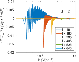
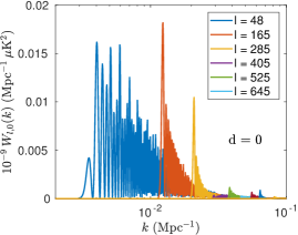
The matrix 𝐖𝐖\mathbf{W}, which relates a given modulation 𝐠LMsuperscript𝐠𝐿𝑀\mathbf{g}^{LM} to the BipoSH coefficients 𝐀LMsuperscript𝐀𝐿𝑀\mathbf{A}^{LM}, has a non-trivial kernel, so the matrix equation (2.10) cannot be inverted to obtain the required 𝐠LMsuperscript𝐠𝐿𝑀\mathbf{g}^{LM}. Physically, this is due to projection effects wherein one mode contributes to many BipoSH coefficients so it is impossible to invert the relation without additional assumptions. This is illustrated in Fig. 1 where different rows of 𝐖𝐖\mathbf{W} are plotted, relating the contribution of a mode k𝑘k to the BipoSH coefficient associated with one of the curves.
Refer to caption
Refer to caption
Figure 1: The transfer functions Wpksubscript𝑊𝑝𝑘W_{pk} relating gkLMsubscriptsuperscript𝑔𝐿𝑀𝑘g^{LM}_{k} to AdLMsubscriptsuperscript𝐴𝐿𝑀𝑑A^{LM}_{\ell d} for d=0𝑑0d=0 (left panel) and d=2𝑑2d=2 (right panel) and representative choices of the multipole \ell. As a rule of thumb, the maxima are near k=η01/14000Mpc1𝑘superscriptsubscript𝜂0114000superscriptMpc1k=\ell\eta_{0}^{-1}\approx\ell/14000\,\mathrm{Mpc^{-1}}, where η0subscript𝜂0\eta_{0} is the conformal time today.

In order to proceed further, this deconvolution problem needs regularisation. We opt to choose that solution 𝐠^^𝐠\hat{\mathbf{g}} amongst the multitude of otherwise equally likely solutions which has the least ‘roughness’ R(𝐠)𝑅𝐠R(\mathbf{g}). This is defined, in the continuous case, as

R(g)=LM(dk(dRegLM(k)dlogk)2+dk(dImgLM(k)dlogk)2),𝑅𝑔subscript𝐿𝑀differential-d𝑘superscriptdResubscript𝑔𝐿𝑀𝑘d𝑘2differential-d𝑘superscriptdImsubscript𝑔𝐿𝑀𝑘d𝑘2\displaystyle R({g})=\sum_{LM}\left(\int\mathrm{d}k\left(\frac{\mathrm{d}\,\mathrm{Re}\,g_{LM}(k)}{\mathrm{d}\log k}\right)^{2}+\int\mathrm{d}k\left(\frac{\mathrm{d}\,\mathrm{Im}\,g_{LM}(k)}{\mathrm{d}\log k}\right)^{2}\right), (2.14)

while, in the discrete case, it is

R(𝐠)𝑅𝐠\displaystyle R(\mathbf{g}) =𝐠T𝚪𝐠,absentsuperscript𝐠𝑇𝚪𝐠\displaystyle=\mathbf{g}^{T}\mathbf{\Gamma}\mathbf{g}, (2.15)

where

𝚪=𝐈5×5𝚪~=(𝚪~𝚪~𝚪~𝚪~𝚪~) and 𝚪~𝚪tensor-productsubscript𝐈55~𝚪matrix~𝚪missing-subexpressionmissing-subexpressionmissing-subexpressionmissing-subexpressionmissing-subexpression~𝚪missing-subexpressionmissing-subexpressionmissing-subexpressionmissing-subexpressionmissing-subexpression~𝚪missing-subexpressionmissing-subexpressionmissing-subexpressionmissing-subexpressionmissing-subexpression~𝚪missing-subexpressionmissing-subexpressionmissing-subexpressionmissing-subexpressionmissing-subexpression~𝚪 and ~𝚪\displaystyle\mathbf{\Gamma}=\mathbf{I}_{5\times 5}\otimes\mathbf{\tilde{\Gamma}}=\begin{pmatrix}\mathbf{\tilde{\Gamma}}&&&&\\ &\mathbf{\tilde{\Gamma}}&&&\\ &&\mathbf{\tilde{\Gamma}}&&\\ &&&\mathbf{\tilde{\Gamma}}&\\ &&&&\mathbf{\tilde{\Gamma}}\end{pmatrix}\textrm{ and }\mathbf{\tilde{\Gamma}} =𝐃T𝐃=(1112112111).absentsuperscript𝐃𝑇𝐃matrix11121missing-subexpressionmissing-subexpressionmissing-subexpression121missing-subexpressionmissing-subexpressionmissing-subexpression11\displaystyle=\mathbf{D}^{T}\mathbf{D}=\begin{pmatrix}1&-1\\ -1&2&-1\\ &\ddots&\ddots&\ddots\\ &&-1&2&-1\\ &&&-1&1\end{pmatrix}. (2.16)

Here 𝐃𝐃\mathbf{D} is the first-order derivative operator and these are the matrix elements of 𝚪~~𝚪\tilde{\mathbf{\Gamma}} when the grid is evenly spaced in logk𝑘\log k. Note that the roughness penalty function does not couple modulations gLM(k)subscript𝑔𝐿𝑀𝑘g_{LM}(k) with different L,M𝐿𝑀L,M values.

The degree to which the solution should be penalised for this roughness is quantified by the regularisation parameter λ𝜆\lambda. The solution will be that which maximises the likelihood (or, equivalently, minimises the negative log likelihood) subject to the constraint that the roughness has the specific value determined by λ𝜆\lambda through:

𝐠^^𝐠\displaystyle\hat{\mathbf{g}} =min𝐠{2log(𝐠,𝐀~)+λ𝐠T𝚪𝐠}.absentsubscript𝐠2𝐠~𝐀𝜆superscript𝐠𝑇𝚪𝐠\displaystyle=\min_{\mathbf{g}}\,\{-2\log\mathcal{L}(\mathbf{g},\tilde{\mathbf{A}})+\lambda\mathbf{g}^{T}\mathbf{\Gamma}\mathbf{g}\,\}. (2.17)

Here \mathcal{L} denotes the likelihood and 𝐀~~𝐀\tilde{\mathbf{A}} denotes the observed values extracted from the CMB map. The likelihood has been multiplied by 22-2 to match the standard χ2superscript𝜒2\chi^{2} statistic for the case of a Gaussian likelihood.

This approach to deconvolution known as ‘Tikhonov regularisation’ has been widely used in image analysis and can be interpreted as Bayesian inference. In the case with a likelihood \mathcal{L}, the solution eq.(2.17) can be seen as the one that maximises the posterior probability P(𝐠|𝐀~)𝑃conditional𝐠~𝐀P(\mathbf{g}|\tilde{\mathbf{A}}) when the prior probability is given by P(𝐠)=exp(λR(𝐠)/2)𝑃𝐠𝜆𝑅𝐠2P(\mathbf{g})=\exp(-\lambda R(\mathbf{g})/2). If the likelihood is Gaussian and the roughness function a quadratic form, then the posterior probability distribution too will be Gaussian. The inverse covariance matrix of the posterior gives the Hessian which in this case is

Hij(λ)=2gigjlog+λ2Γij,subscript𝐻𝑖𝑗𝜆superscript2subscript𝑔𝑖subscript𝑔𝑗𝜆2subscriptΓ𝑖𝑗\displaystyle H_{ij}(\lambda)=-\frac{\partial^{2}}{\partial g_{i}\partial g_{j}}\log\mathcal{L}+\frac{\lambda}{2}\Gamma_{ij}, (2.18)

so its inverse provides the covariance matrix of the posterior, from which credible intervals may be derived.

Note that the regularisation parameter λ𝜆\lambda appears in the prior and can therefore only come from knowledge about the roughness of 𝐠𝐠\mathbf{g}. As this is lacking a priori, we simply consider a range of values for λ𝜆\lambda and report the results. If the likelihood is Gaussian and the roughness function has a quadratic form then the reconstruction can be performed analytically without resorting to numerical minimisation schemes (e.g. ‘BFGS’ which would be necessary for more complicated likelihoods).

Consider the penalised log-likelihood

Q(λ)𝑄𝜆\displaystyle Q(\lambda) =(𝐖𝐠𝐀~)T𝚺1(𝐖𝐠𝐀~)+λ𝐠T𝚪𝐠.absentsuperscriptsuperscript𝐖𝐠~𝐀𝑇superscript𝚺1superscript𝐖𝐠~𝐀𝜆superscript𝐠𝑇𝚪𝐠.\displaystyle=(\mathbf{W}^{\prime}\mathbf{g}-\tilde{\mathbf{A}})^{T}{\mathbf{\Sigma}}^{-1}(\mathbf{W}^{\prime}\mathbf{g}-\tilde{\mathbf{A}})+\lambda{\mathbf{g}}^{T}\mathbf{\Gamma}\mathbf{g}\textrm{.} (2.19)

The penalised likelihood is maximised for

𝐠^^𝐠\displaystyle\hat{\mathbf{g}} =(𝐖T𝚺1𝐖+λ𝚪)1𝐖T𝚺1𝐀~,absentsuperscriptsuperscript𝐖𝑇superscript𝚺1superscript𝐖𝜆𝚪1superscript𝐖𝑇superscript𝚺1~𝐀\displaystyle=(\mathbf{W}^{\prime T}{\mathbf{\Sigma}}^{-1}\mathbf{W}^{\prime}+\lambda\mathbf{\Gamma})^{-1}\mathbf{W}^{\prime T}{\mathbf{\Sigma}}^{-1}\tilde{\mathbf{A}}, (2.20)

and 𝐇=𝐖T𝚺1𝐖+λ𝚪𝐇superscript𝐖𝑇superscript𝚺1superscript𝐖𝜆𝚪\mathbf{H}=\mathbf{W}^{\prime T}\,{\mathbf{\Sigma}}^{-1}\mathbf{W}^{\prime}+\lambda\mathbf{\Gamma} is the Hessian.

It is also useful to consider the frequentist covariance matrix. It is simply the error in 𝐠^^𝐠\hat{\mathbf{g}} that is induced by the error in the data 𝐀~~𝐀\mathbf{\tilde{A}}. Since 𝐠^^𝐠\hat{\mathbf{g}} and 𝐀~~𝐀\mathbf{\tilde{A}}, are related by a linear transformation (2.20), the (frequentist) covariance matrix of 𝐠𝐠\mathbf{g} viz. 𝚺Fsubscript𝚺F\mathbf{\Sigma}_{\mathrm{F}} is related to the data covariance matrix 𝚺𝚺\mathbf{\Sigma} by a similarity transformation

𝚺F=𝐌𝚺𝐌T,subscript𝚺F𝐌𝚺superscript𝐌𝑇\mathbf{\Sigma}_{\mathrm{F}}=\mathbf{M}\mathbf{\Sigma}\mathbf{M}^{T}, (2.21)

where 𝐌=(𝐖T𝚺1𝐖+λ𝚪)1𝐖T𝚺1𝐌superscriptsuperscript𝐖𝑇superscript𝚺1superscript𝐖𝜆𝚪1superscript𝐖𝑇superscript𝚺1\mathbf{M}=(\mathbf{W}^{\prime T}{\mathbf{\Sigma}}^{-1}\mathbf{W}^{\prime}+\lambda\mathbf{\Gamma})^{-1}\mathbf{W}^{\prime T}{\mathbf{\Sigma}}^{-1}. The confidence intervals (frequentist) given by the square root of the diagonal values of 𝚺Fsubscript𝚺F\mathbf{\Sigma}_{\mathrm{F}} will in general be different from the (Bayesian) credible intervals given by the square root of the diagonal values of 𝐇1superscript𝐇1\mathbf{H}^{-1}. To illutrate this we will provide both in what follows.

3 Setup and tests

3.1 Data and covariance matrix setup

The transfer functions in eq.(2.11) were calculated using a customised version of CAMB [20] adopting the Planck best-fit cosmological model. A total of 2316 bins, evenly distributed in logk𝑘\log k space, were used to approximate g2M(k)subscript𝑔2𝑀𝑘g_{2M}(k) in the range from kmin7×106Mpc1similar-tosubscript𝑘min7superscript106superscriptMpc1k_{\mathrm{min}}\sim 7\times 10^{-6}\,\mathrm{Mpc}^{-1} to kmax0.4Mpc1similar-tosubscript𝑘max0.4superscriptMpc1k_{\mathrm{max}}\sim 0.4\,\mathrm{Mpc}^{-1}.

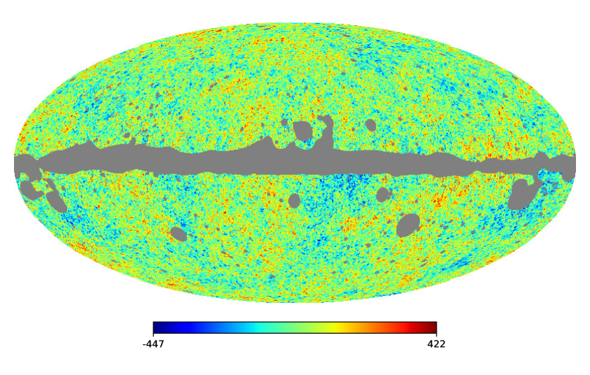
Since statistical anisotropies can also be induced by the instrument itself, due to e.g. non-circular beam effects, pointing errors etc., or by astrophysical foregrounds (see e.g. refs.[21, 22]), we used the most realistic simulations of the instrument and sky, viz. 999 Planck Full Focal Plane (FFP9) simulations [17] to estimate the uncertainties on the extracted BipoSH coefficients. The simulated sky maps were masked using the Planck SMICA mask (COM_Mask_CMB-confidence-Tmask-IQU-smica_1024_R2.02-full with Nside=1024subscript𝑁side1024N_{\mathrm{side}}=1024) [23] shown in grey in Fig. 2.

Refer to caption
Figure 2: The masked PR2–2015 SMICA temperature map in units of μ𝜇\muK.

From the spherical harmonics of the cut sky map bmsubscript𝑏𝑚b_{\ell m}, using eq.(2.5) and eq.(2.6), we then compute the BipoSH coefficients in the following way:

A^LM=1C00L02L+1(2+1)(2+1)mmb^mb^m(1)mCmmLM.subscriptsuperscript^𝐴𝐿𝑀superscript1subscriptsuperscript𝐶𝐿00superscript02𝐿1212superscript1subscript𝑚superscript𝑚subscript^𝑏𝑚subscriptsuperscript^𝑏superscriptsuperscript𝑚superscript1superscript𝑚subscriptsuperscript𝐶𝐿𝑀𝑚superscriptsuperscript𝑚\displaystyle\hat{A}^{LM}_{\ell\ell^{\prime}}=\frac{1}{C^{L0}_{\ell 0\ell^{\prime}0}}\sqrt{\frac{2L+1}{(2\ell+1)(2\ell^{\prime}+1)}}\sum_{mm^{\prime}}\hat{b}_{\ell m}\hat{b}^{\ast}_{\ell^{\prime}m^{\prime}}(-1)^{m^{\prime}}C^{LM}_{\ell m\ell^{\prime}-m^{\prime}}. (3.1)

Lost power was accounted for by multiplying the coefficients by 1/fsky1.176similar-to1subscript𝑓sky1.1761/f_{\mathrm{sky}}\sim 1.176, where fskysubscript𝑓skyf_{\mathrm{sky}} is the available sky fraction 85%similar-toabsentpercent85\sim 85\%.

The BipoSH coefficients A+d2Msubscriptsuperscript𝐴2𝑀𝑑A^{2M}_{\ell~{}\ell+d} were binned with bin size Δ=30Δ30\Delta\ell=30 and weighted by (+1)1\ell(\ell+1), yielding averaged BipoSH coefficients Abb+d2Msubscriptsuperscript𝐴2𝑀subscript𝑏subscript𝑏𝑑A^{2M}_{\ell_{b}~{}\ell_{b}+d} in effective multipoles bsubscript𝑏\ell_{b}. Specifically, a matrix 𝐁𝐁\mathbf{B} was defined with elements

Bbsubscript𝐵subscript𝑏\displaystyle B_{\ell_{b}\ell} =(+1)b(+1),absent1subscript𝑏1\displaystyle=\frac{\ell(\ell+1)}{\sum_{\ell\in b}\ell(\ell+1)}, (3.2)

where b𝑏b is the set of multipoles in the bin. The effective multipoles are then b=𝐁subscriptbold-ℓ𝑏𝐁bold-ℓ\boldsymbol{\ell}_{b}=\mathbf{B}\boldsymbol{\ell} with effective BipoSH coefficients Abb+d2M=BbA+d2Msubscriptsuperscript𝐴2𝑀subscript𝑏subscript𝑏𝑑subscriptsubscript𝐵subscript𝑏subscriptsuperscript𝐴2𝑀𝑑A^{2M}_{\ell_{b}~{}\ell_{b}+d}=\sum_{\ell}B_{\ell_{b}\ell}A^{2M}_{\ell~{}\ell+d}.

We remind the reader of the collective variable q𝑞q which compresses the full index structure that would otherwise comprise of M𝑀M, bsubscript𝑏\ell_{b}, d𝑑d and whether the real or imaginary part of the BipoSH coefficient is considered. The ordering of q𝑞q is such that d𝑑d is iterated over first, then over bsubscript𝑏\ell_{b}, then over M𝑀M, with real parts first and then imaginary parts such that the ordering of the outermost structure is

(M=0,ReM=1,ReM=2,ImM=1,ImM=2)formulae-sequence𝑀0formulae-sequenceRe𝑀1formulae-sequenceRe𝑀2formulae-sequenceImM1ImM2\displaystyle(M=0,\mathrm{Re}\,M=1,\mathrm{Re}\,M=2,\mathrm{Im}\,\mathrm{M}=1,\mathrm{Im}\,\mathrm{M}=2) (3.3)

and within each of the five cells, Ab,b2Msubscriptsuperscript𝐴2𝑀subscript𝑏subscript𝑏A^{2M}_{\ell_{b},\ell_{b}} precedes Ab,b+22Msubscriptsuperscript𝐴2𝑀subscript𝑏subscript𝑏2A^{2M}_{\ell_{b},\ell_{b}+2}.

We compute the mean BipoSH coefficient A¯q2M=Nsim1n=1NsimAq2M(n)superscriptsubscript¯𝐴𝑞2𝑀superscriptsubscript𝑁sim1superscriptsubscript𝑛1subscript𝑁simsubscriptsuperscript𝐴2𝑀𝑞𝑛\bar{A}_{q}^{2M}=N_{\mathrm{sim}}^{-1}\sum_{n=1}^{N_{\mathrm{sim}}}A^{2M}_{q}(n) where Nsim=999subscript𝑁sim999N_{\mathrm{sim}}=999 in this case and the number in the parentheses labels the realisation. Next we compute the covariance matrix:

ΣqqsubscriptΣ𝑞superscript𝑞\displaystyle\Sigma_{qq^{\prime}} =(AqA¯q)(AqA¯q)=1Nsim1n=1Nsim(Aq(n)A¯q)(Aq(n)A¯q),absentdelimited-⟨⟩subscript𝐴𝑞subscript¯𝐴𝑞subscript𝐴superscript𝑞subscript¯𝐴superscript𝑞1subscript𝑁sim1superscriptsubscript𝑛1subscript𝑁simsubscript𝐴𝑞𝑛subscript¯𝐴𝑞subscript𝐴superscript𝑞𝑛subscript¯𝐴superscript𝑞\displaystyle=\langle(A_{q}-\bar{A}_{q})(A_{q^{\prime}}-\bar{A}_{q^{\prime}})\rangle=\frac{1}{N_{\mathrm{sim}}-1}\sum_{n=1}^{N_{\mathrm{sim}}}(A_{q}(n)-\bar{A}_{q})(A_{q^{\prime}}(n)-\bar{A}_{q^{\prime}})\mathrm{,} (3.4)

which, when expanded in the individual components, reads

𝚺=((𝐀20𝐀¯20)(𝐀20𝐀¯20)T(𝐀20𝐀¯20)(Im𝐀22Im𝐀¯22)T(Re𝐀21Re𝐀¯21)(𝐀20𝐀¯20)T(Im𝐀22Im𝐀¯22)(Im𝐀22Im𝐀¯22)T)𝚺matrixdelimited-⟨⟩superscript𝐀20superscript¯𝐀20superscriptsuperscript𝐀20superscript¯𝐀20𝑇missing-subexpressionmissing-subexpressiondelimited-⟨⟩superscript𝐀20superscript¯𝐀20superscriptImsuperscript𝐀22Imsuperscript¯𝐀22𝑇delimited-⟨⟩Resuperscript𝐀21Resuperscript¯𝐀21superscriptsuperscript𝐀20superscript¯𝐀20𝑇missing-subexpressionmissing-subexpressionmissing-subexpressionmissing-subexpressionmissing-subexpressionmissing-subexpressiondelimited-⟨⟩Imsuperscript𝐀22Imsuperscript¯𝐀22superscriptImsuperscript𝐀22Imsuperscript¯𝐀22𝑇\displaystyle\mathbf{\Sigma}=\begin{pmatrix}\langle(\mathbf{A}^{20}-\bar{\mathbf{A}}^{20})({\mathbf{A}^{20}}-\bar{\mathbf{A}}^{20})^{T}\rangle&&\cdots&&\langle(\mathbf{A}^{20}-\bar{\mathbf{A}}^{20})(\mathrm{Im}\,{\mathbf{A}^{22}}-\mathrm{Im}\,{\bar{\mathbf{A}}^{22}})^{T}\rangle\\ \langle(\mathrm{Re}\,\mathbf{A}^{21}-\mathrm{Re}\,\bar{\mathbf{A}}^{21})({\mathbf{A}^{20}}-\bar{\mathbf{A}}^{20})^{T}\rangle&\ddots&&&\\ \vdots&&&&\langle(\mathrm{Im}\,\mathbf{A}^{22}-\mathrm{Im}\,\bar{\mathbf{A}}^{22})(\mathrm{Im}\,{\mathbf{A}^{22}}-\mathrm{Im}\,{\bar{\mathbf{A}}^{22}})^{T}\rangle\end{pmatrix} (3.5)

and invert this to obtain the inverse covariance matrix 𝚺1superscript𝚺1{\mathbf{\Sigma}}^{-1} which was used to finally construct the likelihood:

2log(𝐠,𝐀~)2𝐠~𝐀\displaystyle-2\log\mathcal{L}(\mathbf{g},\tilde{\mathbf{A}}) =(𝐖𝐠𝐀~+𝐀¯)T𝚺1(𝐖𝐠𝐀~+𝐀¯).absentsuperscriptsuperscript𝐖𝐠~𝐀¯𝐀𝑇superscript𝚺1superscript𝐖𝐠~𝐀¯𝐀\displaystyle=(\mathbf{W}^{\prime}\mathbf{g}-\tilde{\mathbf{A}}+\bar{\mathbf{A}})^{T}{\mathbf{\Sigma}}^{-1}(\mathbf{W}^{\prime}\mathbf{g}-\tilde{\mathbf{A}}+\bar{\mathbf{A}}). (3.6)

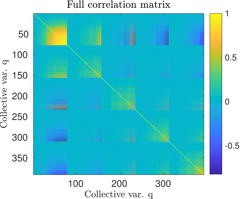
The covariance matrix 𝚺𝚺\mathbf{\Sigma} was found to have non-neglible off-diagonal values despite the Δ=30Δ30\Delta\ell=30 binning. For b>600subscript𝑏600\ell_{b}>600 and in particular in the subspace corresponding to the covariance of M=0𝑀0M=0, the bins are strongly correlated. The full correlation matrix is shown in Fig. 3. There are strong correlations as well as anticorrelations for different M𝑀M, most pronounced for correlations with M=0𝑀0M=0. It is therefore necessary to include the full covariance matrix in the likelihood.
Refer to caption
Figure 3: Full correlation matrix. Collective variable q𝑞q now also includes M=0,1,2𝑀012M=0,1,2 and real and imaginary parts, listing first the real parts and then the imaginary parts: real pt. M=0𝑀0M=0, real pt. M=1𝑀1M=1, real pt. M=2𝑀2M=2, imaginary pt. M=1𝑀1M=1, imaginary pt. M=2𝑀2M=2.

3.2 Gaussianity test

Since the likelihood is the probability of observing the data 𝐀~~𝐀\tilde{\mathbf{A}} in the Planck best-fit ΛΛ\LambdaCDM cosmology with an instrument that has the characteristics modelled by the FFP simulations and its foregrounds, eq.(3.6) is valid only if that is indeed what the model predicts. However since that likelihood would be very involved given the complex nature of the FFP simulations, we instead inspected the distributions of the BipoSH coefficients of the 999 realisations.

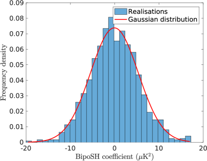
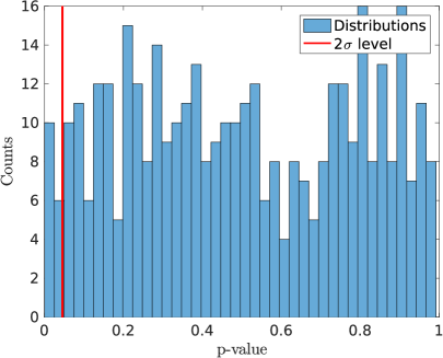
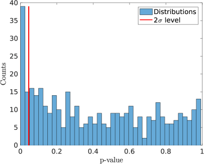
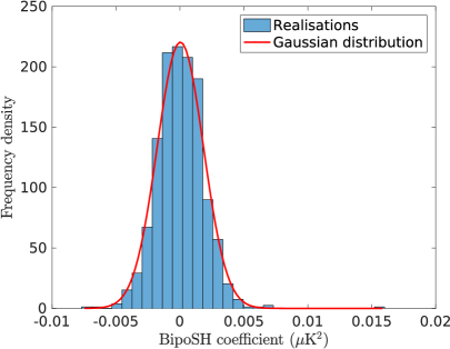
To test the normality of the distribution of BipoSH coefficients from the FFP simulations, an Anderson-Darling test [24] was performed on each distribution of Abb+d2Msubscriptsuperscript𝐴2𝑀subscript𝑏subscript𝑏𝑑A^{2M}_{\ell_{b}~{}\ell_{b}+d}. The details of this test, which is sensitive to the tail of a distribution, can be found in Appendix E. The resulting p-values are shown in Fig. 4 which also shows a typical distribution.
Refer to caption
Refer to caption
Figure 4: Tests of normality of distributions of the BipoSH coefficients Abb+d2Msubscriptsuperscript𝐴2𝑀subscript𝑏subscript𝑏𝑑A^{2M}_{\ell_{b}~{}\ell_{b}+d}. In the left panel, a histogram of p-values of Anderson-Darling tests on the distributions is shown with a vertical (red) line marking the 2σ2𝜎2\sigma significance level. The right panel shows a histogram of 999 realisations of a particular BipoSH coefficient A76762,0subscriptsuperscript𝐴207676A^{2,0}_{76~{}76}, with a Gaussian distribution superimposed.

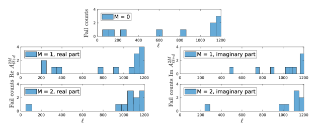
It is seen that at 2σ2𝜎2\sigma significance, 52 out of 390 i.e. 13.3% of the distributions did not pass the Anderson-Darling test. Of these, 41 come from multipoles >700700\ell>700 as seen in Fig. 5.

Refer to caption
Figure 5: Counts of distributions of the BipoSH coefficients A+d2Msubscriptsuperscript𝐴2𝑀𝑑A^{2M}_{\ell~{}\ell+d} failing the Anderson-Darling test at 2σ2𝜎2\sigma significance level. The distributions of the real and imaginary part are shown, respectively, in the left and right panel. Note the larger count for >10001000\ell>1000.

An example of distribution that failed the test is shown in Fig. 6. An outlier is present that causes the distribution, which would otherwise be well modelled by a normal distribution, to fail the test. It turns out that the mask used on the skymap is responsible for most test failures. This is demonstrated by the fact that when the Anderson-Darling test is run on unmasked sky realisations, only 16 distributions failed, compared to 52 for the masked sky. (Of course, a certain number is expected to fail in any case as only a finite number of simulations have been run.) Despite this problem of outliers for >700700\ell>700, the Gaussian model of the likelihood seems justified and we adopt it as our likelihood.
Refer to caption
Refer to caption
Figure 6: The left panel shows a distribution of realisations of the BipoSH coefficient A118511852,2subscriptsuperscript𝐴2211851185A^{2,2}_{1185~{}1185} which fail the Anderson-Darling test due to an outlier at 0.015μsimilar-toabsent0.015𝜇\sim 0.015~{}\muK2. In the right panel the normality test is repeated on unmasked realisations — now only 16 distributions fail the Anderson-Darling test, compared to 52 when the mask is used.

3.3 Mock data tests

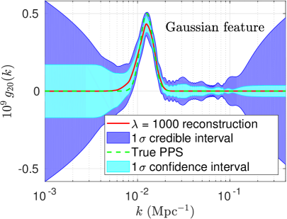
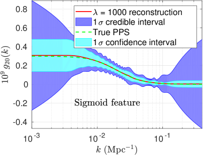
To test our approach, the BipoSH coefficients of known quadrupole modulations were calculated. The quadrupole modulations without noise were then reconstructed from these BipoSH coefficients using eq.(2.20). The uncertainties associated with the reconstructions were taken to be those expected from an experiment that is properly modelled by the FFP simulations, including cosmic variance. The results for two different assumed modulations of g20(k)subscript𝑔20𝑘g_{20}(k) are shown in Fig. 7. One is a Gaussian

g20(k)=aexp((log10(k/k0))2/q2),subscript𝑔20𝑘𝑎superscriptsubscript10𝑘subscript𝑘02superscript𝑞2g_{20}(k)=a\exp(-(\log_{10}(k/k_{0}))^{2}/q^{2}), (3.7)

with a=0.5𝑎0.5a=0.5 , k0=1.26×10²Mpc1subscript𝑘01.26superscript102superscriptMpc1k_{0}=1.26\times 10^{-2}\,\mathrm{Mpc}^{-1} and q=0.1𝑞0.1q=0.1, while the other is a sigmoid

g20(k)=aexp((log10(k/k0))/q)/(1+exp((log10(k/k0))/q)),subscript𝑔20𝑘𝑎subscript10𝑘subscript𝑘0𝑞1subscript10𝑘subscript𝑘0𝑞g_{20}(k)=a\exp(-(\log_{10}(k/k_{0}))/q)/(1+\exp(-(\log_{10}(k/k_{0}))/q)), (3.8)

with k0=2×10²Mpc1subscript𝑘02superscript102superscriptMpc1k_{0}=2\times 10^{-2}\,\mathrm{Mpc}^{-1}, q=0.2𝑞0.2q=0.2 and a=0.3𝑎0.3a=0.3. Although slight biases towards smoother spectra are visible, our reconstructions capture the features well and the credible intervals are seen to be quite distinct from zero power.
Refer to caption
Refer to caption
Figure 7: Reconstruction of noise-free test spectra with regularisation parameter λ=1000𝜆1000\lambda=1000. Purple bands indicate the uncertainty in the posterior probability which reflects the uncertainties associated with the experiment — cosmic variance as well as the choice of prior. Cyan bands indicate the scatter in the reconstruction due to scatter in the data. The reconstruction (full red line) matches well the true spectrum (dotted green line) and is clearly distinguishable from no power. The left and right panels show the reconstruction of a Gaussian (3.7) and sigmoid (3.8) feature respectively.

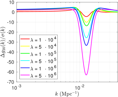
The reconstruction parameter will be biased against features if a high value of the regularisation parameter is chosen, as is evident in the Bayesian view of Tikhonov regularisation where λ𝜆\lambda controls the roughness of the prior. The bias relative to the uncertainty is demonstrated in Fig. 8 where the Gaussian feature of Fig. 7 is reconstructed with different choices of λ𝜆\lambda. The least biased curve is the one with the smallest λ𝜆\lambda. Lowering λ𝜆\lambda increases the uncertainty however, so that too small a value makes the reconstruction uninformative. Clearly this determines an optimal value of λ𝜆\lambda for reconstruction, as has been discussed in ref.[14].
Refer to caption
Figure 8: Bias in reconstruction of a Gaussian feature: Starting with λ=104𝜆superscript104\lambda=10^{4} (red) and ending with λ=5×10⁶𝜆5superscript106\lambda=5\times 10^{6} (blue), a bias is observed with the lowest λ𝜆\lambda being least biased. The plot shows the difference between the true and the reconstructed spectrum relative to the uncertainty.

4 Results

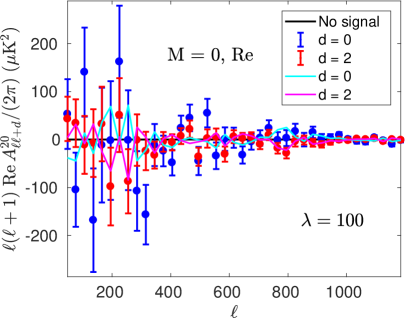
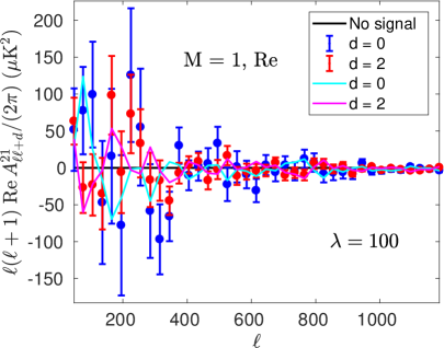
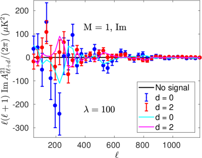
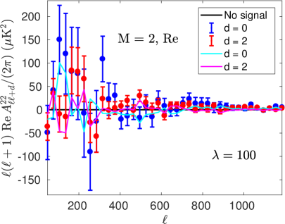
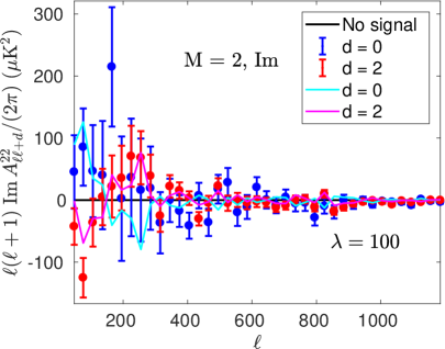
We look for a modulation in the masked PR2–2015 SMICA intensity map222The full name is COM_CMB_IQU-smica_1024_R2.01_full with Nside=1024subscript𝑁side1024N_{\mathrm{side}}=1024 [23]. shown in Fig. 2. The BipoSH coefficients 𝐀~2Msuperscript~𝐀2𝑀\tilde{\mathbf{A}}^{2M} are calculated using eq.(3.1) for M=0,1,2𝑀012M=0,1,2 and d=0,2𝑑02d=0,2 in the range 30120030120030\leq\ell\leq 1200. There is only a real part for M=0𝑀0M=0 but M=1,2𝑀12M=1,2 also have imaginary parts. Fig. 9 shows the bias-corrected data points 𝐀~2M𝐀¯2Msuperscript~𝐀2𝑀superscript¯𝐀2𝑀\tilde{\mathbf{A}}^{2M}-\bar{\mathbf{A}}^{2M}.

Refer to caption
Refer to caption
Refer to caption
Refer to caption
Refer to caption
Figure 9: Real and imaginary parts of the corrected BipoSH coefficients A,+d2Msubscriptsuperscript𝐴2𝑀𝑑A^{2M}_{\ell,\ell+d} of the masked PR2–2015 SMICA map in bins of Δ=30Δ30\Delta\ell=30, with A,2Msubscriptsuperscript𝐴2𝑀A^{2M}_{\ell,\ell} (d=0𝑑0d=0) in blue, and A,+22Msubscriptsuperscript𝐴2𝑀2A^{2M}_{\ell,\ell+2} (d=2𝑑2d=2) in red. The BipoSH coefficients associated with the quadrupole modulation reconstructed (λ=100𝜆100\lambda=100) from data (magenta lines for d=0𝑑0d=0 and cyan lines for d=2𝑑2d=2) are superimposed.

4.1 Scale-independent quadrupole modulation

The best-fit constant spectrum g2Msubscript𝑔2𝑀g_{2M\star} can be defined via the equation:333The numerical factor cancels the 4π4𝜋\sqrt{4\pi} in eq.(1.2) and enables a direct comparison with related work [12].

g2M(k)=(4π)1/2g2M𝒫(k),subscript𝑔2𝑀𝑘superscript4𝜋12subscript𝑔2𝑀𝒫𝑘g_{2M}(k)=(4\pi)^{-1/2}g_{2M\star}\mathcal{P}(k), (4.1)

where the best-fit isotropic spectrum is taken to be 𝒫(k)=A(k/k)ns1𝒫𝑘𝐴superscript𝑘subscript𝑘subscript𝑛𝑠1\mathcal{P}(k)=A(k/k_{\ast})^{n_{s}-1} with k=0.05Mpc1subscript𝑘0.05superscriptMpc1k_{\ast}=0.05\,\mathrm{Mpc^{-1}}, A=2.198𝐴2.198A=2.198 and ns=0.9655subscript𝑛s0.9655n_{\mathrm{s}}=0.9655 (best-fit parameters from Planck TT+lowP) [25]. We look for the g2Msubscript𝑔2𝑀g_{2M\star}, collectively denoted 𝜶𝜶\boldsymbol{\alpha}, which maximises the likelihood (3.6) which is in this case,

2log=((4π)1/2𝐖𝐐𝜶𝐀~+𝐀¯)T𝚺1((4π)1/2𝐖𝐐𝜶𝐀~+𝐀¯)2superscriptsuperscript4𝜋12superscript𝐖𝐐𝜶~𝐀¯𝐀𝑇superscript𝚺1superscript4𝜋12superscript𝐖𝐐𝜶~𝐀¯𝐀\displaystyle-2\log\mathcal{L}=((4\pi)^{-1/2}\,\mathbf{W}^{\prime}\mathbf{Q}\boldsymbol{\alpha}-\tilde{\mathbf{A}}+\bar{\mathbf{A}})^{T}\mathbf{\Sigma}^{-1}((4\pi)^{-1/2}\,\mathbf{W}^{\prime}\mathbf{Q}\boldsymbol{\alpha}-\tilde{\mathbf{A}}+\bar{\mathbf{A}}) (4.2)

where

𝐐=𝐈5×5𝐩=(𝐩𝐩)𝐐tensor-productsubscript𝐈55𝐩matrix𝐩missing-subexpressionmissing-subexpressionmissing-subexpressionmissing-subexpressionmissing-subexpressionmissing-subexpression𝐩\displaystyle\mathbf{Q}=\mathbf{I}_{5\times 5}\otimes\mathbf{p}=\begin{pmatrix}\mathbf{p}&&\\ &\ddots&\\ &&\mathbf{p}\end{pmatrix} (4.3)

is a block matrix made of the isotropic primordial power spectrum 𝐩𝐩\mathbf{p} stacked five times. The maximum likelihood estimate is obtained by differentiating with respect to 𝜶𝜶\boldsymbol{\alpha}, setting the expression equal to zero and isolating 𝜶𝜶\boldsymbol{\alpha}:

g^2Msubscript^𝑔2𝑀\displaystyle\hat{g}_{2M\star} 𝜶=4π𝐉1𝐐T𝐖T𝚺1(𝐀~𝐀¯)absent𝜶4𝜋superscript𝐉1superscript𝐐𝑇superscript𝐖𝑇superscript𝚺1~𝐀¯𝐀\displaystyle\equiv\boldsymbol{\alpha}=\sqrt{4\pi}\mathbf{J}^{-1}\mathbf{Q}^{T}\mathbf{W}^{\prime T}\mathbf{\Sigma}^{-1}(\tilde{\mathbf{A}}-\bar{\mathbf{A}}) (4.4)

where

𝐉=𝐐T(𝐖)T𝚺1𝐖𝐐.𝐉superscript𝐐𝑇superscriptsuperscript𝐖𝑇superscript𝚺1superscript𝐖𝐐\displaystyle\mathbf{J}=\mathbf{Q}^{T}(\mathbf{W}^{\prime})^{T}\mathbf{\Sigma}^{-1}\mathbf{W}^{\prime}\mathbf{Q}. (4.5)

The uncertainty of g2Msubscript𝑔2𝑀g_{2M\star} is just the inverse Hessian, i.e., the inverse of the double derivative of log-\log\mathcal{L} with respect to g2Msubscript𝑔2𝑀g_{2M\star}, which in this case is:

𝐇1superscript𝐇1\displaystyle\mathbf{H}^{-1} =4π𝐉1.absent4𝜋superscript𝐉1\displaystyle=4\pi\mathbf{J}^{-1}. (4.6)

When we quote the 1D uncertainties they correspond to the square root of the diagonal entries of the inverse Hessian:

σg2Mσi=4π(J1)iisubscript𝜎subscript𝑔2𝑀subscript𝜎𝑖4𝜋subscriptsuperscript𝐽1𝑖𝑖\displaystyle\sigma_{g_{2M\star}}\equiv\sigma_{i}=\sqrt{4\pi(J^{-1})_{ii}} (4.7)

where Jiisubscript𝐽𝑖𝑖J_{ii} are the diagonal values of 𝐉𝐉\mathbf{J} and i𝑖i is the index running from 111 (Reg20Resubscript𝑔20\mathrm{Re}\,g_{20\star}) to 555 (Img22Imsubscript𝑔22\mathrm{Im}\,g_{22\star}).

Our results are summarised in Table 1. Both Reg20Resubscript𝑔20\mathrm{Re}\,g_{20\star} and Reg22Resubscript𝑔22\mathrm{Re}\,g_{22\star} appear to be higher than expected, over twice the expected value. We perform the p-value test later.

M𝑀M 102×Reg2Msuperscript102Resubscript𝑔2𝑀10^{2}\times\mathrm{Re}\,{g}_{2M\star} 102×Img2Msuperscript102Imsubscript𝑔2𝑀10^{2}\times\mathrm{Im}\,{g}_{2M\star}
00 0.76±0.34plus-or-minus0.760.340.76\pm 0.34
111 0.05±0.20plus-or-minus0.050.200.05\pm 0.20 0.14±0.20plus-or-minus0.140.20-0.14\pm 0.20
222 0.48±0.21plus-or-minus0.480.210.48\pm 0.21 0.09±0.20plus-or-minus0.090.200.09\pm 0.20
Table 1: Results for the best-fit constant quadrupole modulation g2Msubscript𝑔2𝑀g_{2M\star}, eq.(4.1).

4.2 Power-law quadrupole modulations

We also test for a power-law quadrupole modulation of the form

g2M(k)=4πg15(kk)q𝒫(k)Y2M(θ,ϕ),subscript𝑔2𝑀𝑘4𝜋subscript𝑔15superscript𝑘subscript𝑘𝑞𝒫𝑘subscriptsuperscript𝑌2𝑀𝜃italic-ϕg_{2M}(k)=\frac{4\sqrt{\pi}g_{\ast}}{15}\left(\frac{k}{k_{\ast}}\right)^{q}\mathcal{P}(k)Y^{\ast}_{2M}(\theta,\phi), (4.8)

where 𝒫(k)𝒫𝑘\mathcal{P}(k) is the best fit isotropic spectrum and the coefficient is chosen to ensure a direct comparison with the Planck collaboration’s results [13]. In real space, this corresponds to a quadrupole modulation (𝐤^𝐧^)2proportional-toabsentsuperscript^𝐤^𝐧2\propto(\hat{\mathbf{k}}\cdot\hat{\mathbf{n}})^{2} where 𝐧^=(θ,ϕ)^𝐧𝜃italic-ϕ\hat{\mathbf{n}}=(\theta,\phi) is a unit vector in the direction of the hot spot. The posterior distribution of the parameters (g,θ,ϕ)subscript𝑔𝜃italic-ϕ(g_{\ast},\theta,\phi) is estimated using the Metropolis-Hastings algorithm with flat priors on the angles and a flat prior on gsubscript𝑔g_{\ast} in the range 10102g1010superscript102subscript𝑔10-10\leq 10^{2}g_{\ast}\leq 10. The results are shown in Table 2.

q𝑞q 22-2 11-1 00 111 222
102g<0superscript102subscript𝑔010^{2}{g}_{\ast}<0 0.00±0.13plus-or-minus0.000.13-0.00\pm 0.13 0.560.39+0.40subscriptsuperscript0.560.400.39-0.56^{+0.40}_{-0.39} 0.740.33+0.34subscriptsuperscript0.740.340.33-0.74^{+0.34}_{-0.33} 0.470.21+0.22subscriptsuperscript0.470.220.21-0.47^{+0.22}_{-0.21} 0.260.12+0.13subscriptsuperscript0.260.130.12-0.26^{+0.13}_{-0.12}
102g>0superscript102subscript𝑔010^{2}{g}_{\ast}>0 0.820.39+0.38subscriptsuperscript0.820.380.390.82^{+0.38}_{-0.39} 0.630.35+0.33subscriptsuperscript0.630.330.350.63^{+0.33}_{-0.35} 0.270.18+0.17subscriptsuperscript0.270.170.180.27^{+0.17}_{-0.18} 0.140.10+0.10subscriptsuperscript0.140.100.100.14^{+0.10}_{-0.10}
Table 2: Results for the best-fit power-law quadrupole modulations of the form of eq.(4.8) for different power law indices.

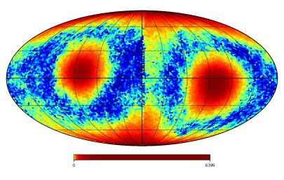
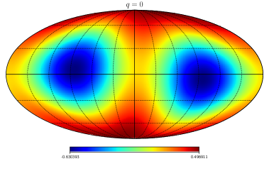
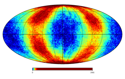
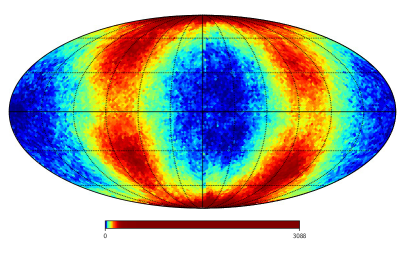
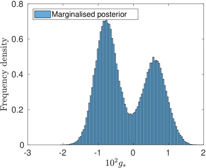
The credible intervals are such that 68.2%percent68.268.2\% of the probability is contained in the quoted ranges. The posterior distribution of gsubscript𝑔g_{\ast} found after marginalising over the directions θ,ϕ𝜃italic-ϕ\theta,\phi is shown in Fig. 10 for the case of q=0𝑞0q=0. It is bimodal. A Mollweide projection of the posterior distribution of the direction (θ,ϕ)𝜃italic-ϕ(\theta,\phi) is also shown. Nearly half the total posterior probability (49%percent4949\%) is focussed in the direction (l,b)=(8415+13,712+13)𝑙𝑏subscriptsuperscriptsuperscript841315subscriptsuperscriptsuperscript71312(l,b)=({84^{\circ}}^{+13}_{-15},{7^{\circ}}^{+13}_{-12}) with amplitude 102g=0.740.33+0.34superscript102subscript𝑔subscriptsuperscript0.740.340.3310^{2}g_{\ast}=-0.74^{+0.34}_{-0.33} which correspond to the two lobes. The best-fit positive amplitude is 102g=0.630.35+0.33superscript102subscript𝑔subscriptsuperscript0.630.330.3510^{2}g_{\ast}=0.63^{+0.33}_{-0.35}. The probability distribution of the direction of the positive amplitude modulation g>0subscript𝑔0g_{\ast}>0 is almost uniform in the azimuthal direction, but not in the polar direction. The best-fit here points perpendicular to the Galactic plane b=1.9221+21𝑏subscriptsuperscriptsuperscript1.922121b={1.92^{\circ}}^{+21}_{-21}. This is suggestive of possible contamination of the SMICA map by Galactic foregrounds.
Refer to caption

Refer to caption

Figure 10: The left panel shows the Metropolis-Hastings sampled posterior distribution of 102gsuperscript102subscript𝑔10^{2}g_{\ast} for the scale-independent case q=0𝑞0q=0 assuming a flat prior on 10102g1010superscript102subscript𝑔10-10\leq 10^{2}g_{\ast}\leq 10 and marginalising over the angles θ,ϕ𝜃italic-ϕ\theta,\phi. The posterior distribution is bimodal. The right panel shows the Mollweide projection of the posterior distribution of directions (θ,ϕ)𝜃italic-ϕ(\theta,\phi).

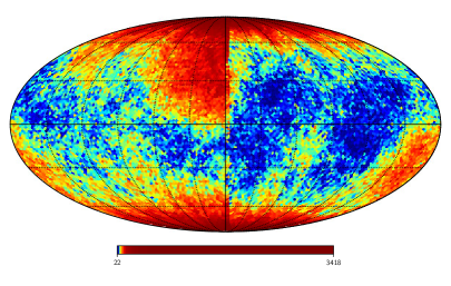
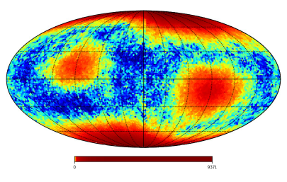
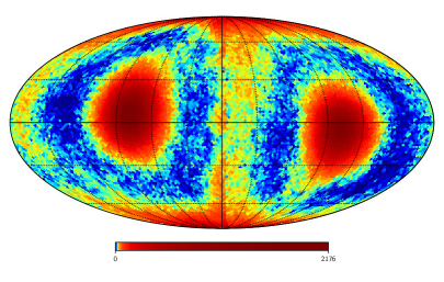
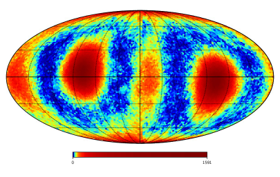
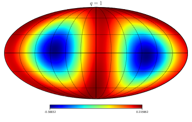
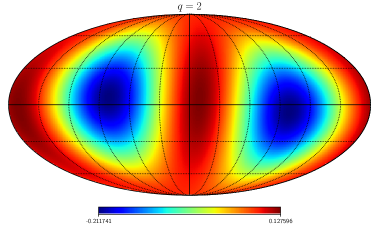
Fig. 11 shows the Mollweide projection of the posterior distributions for the other values of the power-law index q𝑞q.

Refer to caption
Refer to caption
Refer to caption
Refer to caption
Figure 11: Equalised histograms of possible directions of the quadrupole modulation for power law modulations of the form g2M(k)(k/k)qproportional-tosubscript𝑔2𝑀𝑘superscript𝑘subscript𝑘𝑞g_{2M}(k)\propto(k/k_{\ast})^{q} ranging from q=2𝑞2q=-2 (upper left figure) to q=2𝑞2q=2 (centred lower figure) derived from Monte Carlo runs.

Eq.(4.1) can also be generalised to include a power-law quadrupole modulation:

g2M(k)=(4π)1/2g2M(k/k)q𝒫(k),subscript𝑔2𝑀𝑘superscript4𝜋12subscript𝑔2𝑀superscript𝑘subscript𝑘𝑞𝒫𝑘\displaystyle g_{2M}(k)=(4\pi)^{-1/2}g_{2M\star}(k/k_{\ast})^{q}\mathcal{P}(k), (4.9)

with power q𝑞q and amplitude g2Msubscript𝑔2𝑀g_{2M\star}. Unlike the previously considered form (4.8), this allows for the most general quadrupole power law modulation which means that the directions of the two dipoles that a quadrupole can be factorised into need not coincide. The maximum likelihood amplitudes and uncertainties of such modulations are given by the same expressions as those for the constant quadrupole modulation upon replacing the discretised version of 𝒫(k)𝒫𝑘\mathcal{P}(k) (i.e., 𝐩𝐩\mathbf{p} in eqs.(4.4) and (4.6)) with a discretised version of 𝒫(k)(k/k)q𝒫𝑘superscript𝑘subscript𝑘𝑞\mathcal{P}(k)(k/k_{\ast})^{q}. The results are shown in Table 3 and Figure 12. Their statistical significance will be evaluated in Section 5.
Refer to caption
Refer to caption
Refer to caption
Refer to caption
Refer to caption
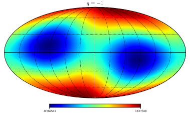
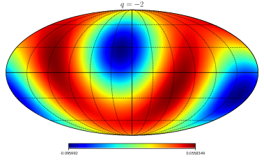
Figure 12: Mollweide projection of the best-fit power law quadrupole modulation g2M(k)𝒫(k)(k/k)qproportional-tosubscript𝑔2𝑀𝑘𝒫𝑘superscript𝑘subscript𝑘𝑞g_{2M}(k)\propto\mathcal{P}(k)(k/k_{\ast})^{q} ranging from q=2𝑞2q=-2 to q=2𝑞2q=2.
M𝑀M 102×Reg2Msuperscript102Resubscript𝑔2𝑀10^{2}\times\mathrm{Re}\,{g}_{2M\star} 102×Img2Msuperscript102Imsubscript𝑔2𝑀10^{2}\times\mathrm{Im}\,{g}_{2M\star} M𝑀M 102×Reg2Msuperscript102Resubscript𝑔2𝑀10^{2}\times\mathrm{Re}\,{g}_{2M\star} 102×Img2Msuperscript102Imsubscript𝑔2𝑀10^{2}\times\mathrm{Im}\,{g}_{2M\star}
q=2𝑞2q=-2 q=2𝑞2q=2
00 0.02±0.12plus-or-minus0.020.120.02\pm 0.12 00 0.13±0.12plus-or-minus0.130.120.13\pm 0.12
111 0.07±0.09plus-or-minus0.070.090.07\pm 0.09 0.02±0.09plus-or-minus0.020.09-0.02\pm 0.09 111 0.00±0.07plus-or-minus0.000.070.00\pm 0.07 0.04±0.07plus-or-minus0.040.07-0.04\pm 0.07
222 0.06±0.09plus-or-minus0.060.09-0.06\pm 0.09 0.05±0.09plus-or-minus0.050.090.05\pm 0.09 222 0.21±0.07plus-or-minus0.210.070.21\pm 0.07 0.07±0.07plus-or-minus0.070.070.07\pm 0.07
q=1𝑞1q=-1 q=1𝑞1q=1
00 0.95±0.39plus-or-minus0.950.390.95\pm 0.39 00 0.33±0.21plus-or-minus0.330.210.33\pm 0.21
111 0.04±0.25plus-or-minus0.040.250.04\pm 0.25 0.30±0.25plus-or-minus0.300.25-0.30\pm 0.25 111 0.02±0.13plus-or-minus0.020.130.02\pm 0.13 0.06±0.12plus-or-minus0.060.12-0.06\pm 0.12
222 0.28±0.26plus-or-minus0.280.260.28\pm 0.26 0.05±0.25plus-or-minus0.050.25-0.05\pm 0.25 222 0.35±0.13plus-or-minus0.350.130.35\pm 0.13 0.11±0.12plus-or-minus0.110.120.11\pm 0.12
Table 3: Power-law quadrupole modulations of the form g2Mg2M(k/k)q𝒫(k)proportional-tosubscript𝑔2𝑀subscript𝑔2𝑀superscript𝑘subscript𝑘𝑞𝒫𝑘g_{2M}\propto g_{2M\star}(k/k_{\ast})^{q}\mathcal{P}(k).

The most general quadrupole is described by two directions, 𝐧^1subscript^𝐧1\hat{\mathbf{n}}_{1} and 𝐧^2subscript^𝐧2\hat{\mathbf{n}}_{2}, and an amplitude gAsubscript𝑔𝐴g_{A} and is of the form gA(𝐤^𝐧1)(𝐤^𝐧^2)subscript𝑔𝐴^𝐤subscript𝐧1^𝐤subscript^𝐧2g_{A}(\hat{\mathbf{k}}\cdot\mathbf{n}_{1})(\hat{\mathbf{k}}\cdot\hat{\mathbf{n}}_{2}) where 𝐤^=(θ,ϕ)^𝐤𝜃italic-ϕ\hat{\mathbf{k}}=(\theta,\phi). This has previously been studied by ref.[26]. The relation between the quadrupole modulations g2Msubscript𝑔2𝑀g_{2M} and the direction is found by decomposing this form into spherical harmonics

g2M=gAdΩ(𝐤^𝐧^1)(𝐤^𝐧^2)Y2M(θ,ϕ).subscript𝑔2𝑀subscript𝑔𝐴differential-dΩ^𝐤subscript^𝐧1^𝐤subscript^𝐧2subscriptsuperscript𝑌2𝑀𝜃italic-ϕ\displaystyle g_{2M}=g_{A}\int\mathrm{d}\Omega\,(\hat{\mathbf{k}}\cdot\hat{\mathbf{n}}_{1})(\hat{\mathbf{k}}\cdot\hat{\mathbf{n}}_{2})Y^{\ast}_{2M}(\theta,\phi). (4.10)

The best-fit quadrupole modulations for the different powers q𝑞q are displayed in Fig. 12, although they are not particularly informative as there are large uncertainties in the directions of 𝐧^1subscript^𝐧1\hat{\mathbf{n}}_{1} and 𝐧^2subscript^𝐧2\hat{\mathbf{n}}_{2} (as seen for the case of the constant quadrupole modulation q=0𝑞0q=0 in Fig. 13).

Refer to caption
Refer to caption
Figure 13: Mollweide projection of equalised histograms of possible directions 𝐧^1subscript^𝐧1\hat{\mathbf{n}}_{1} (left) and 𝐧^2subscript^𝐧2\hat{\mathbf{n}}_{2} (right) of the most general scale-independent quadrupole modulation.

4.3 Non-parametric quadrupole modulations

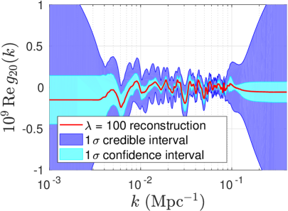
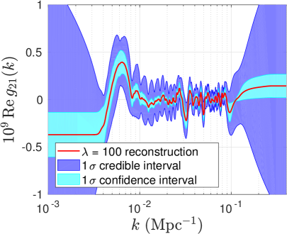
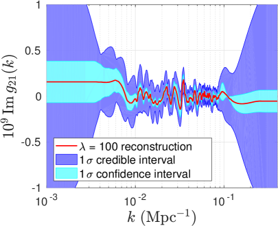
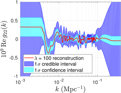
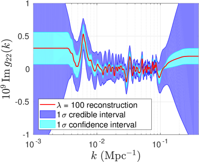
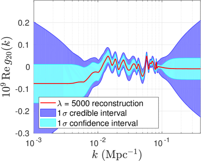
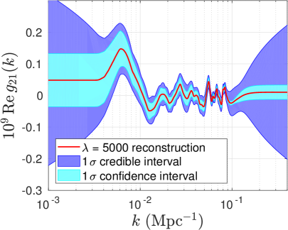
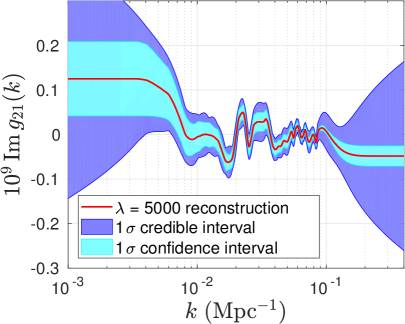
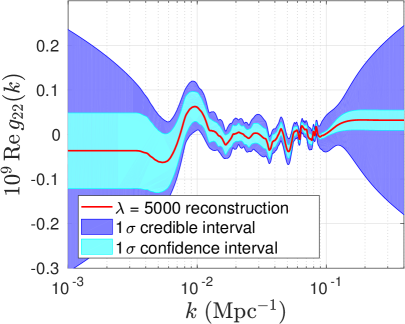
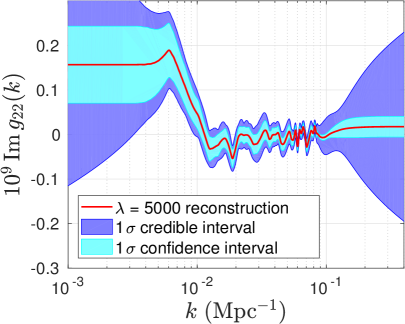
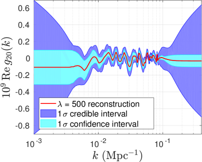
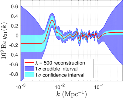
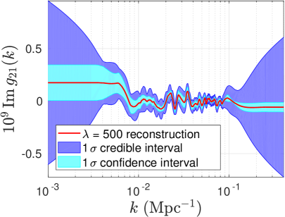
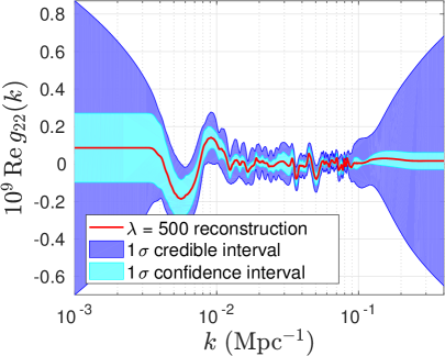
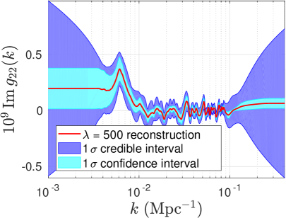
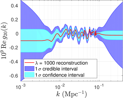
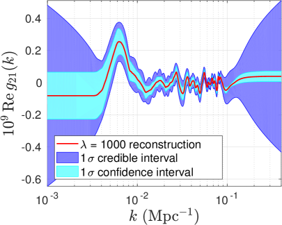
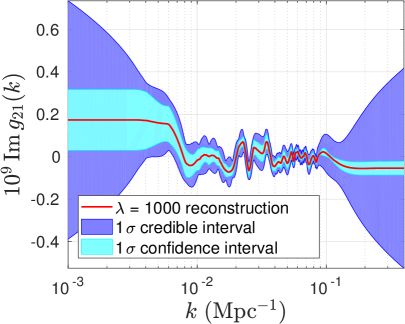
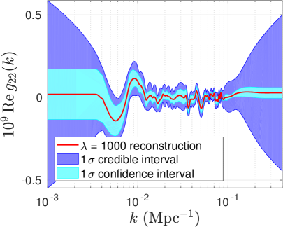
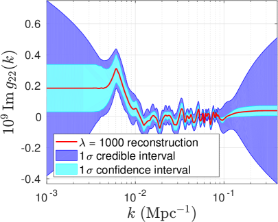
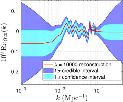
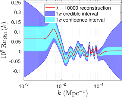
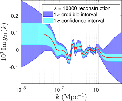
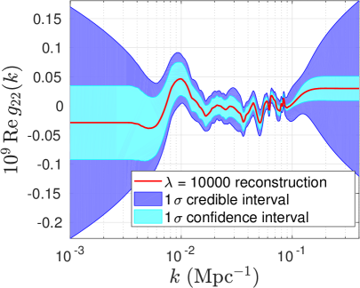
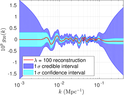
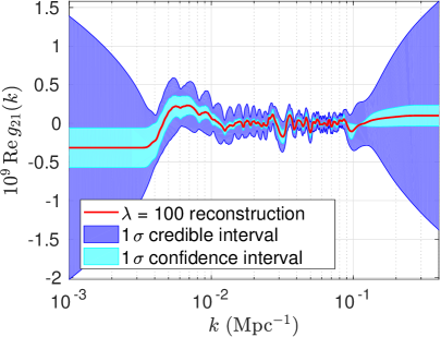
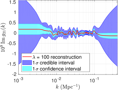
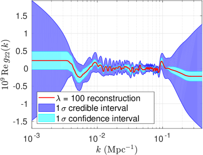
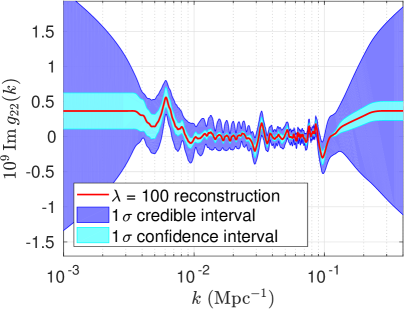
We now present new results concerning a possible scale-dependent quadrupole modulation of the primordial power spectrum. The quadrupole modulation reconstructed using eq.(2.20) from the masked PR2–2015 SMICA temperature map with uncertainties modelled by the masked FFP9 simulations is shown in Fig. 14 for λ=100𝜆100\lambda=100 and in Fig. 16 for λ=5000𝜆5000\lambda=5000. Plots for other choices of λ𝜆\lambda are shown in Appendix C.

Refer to caption
Refer to caption
Refer to caption
Refer to caption
Refer to caption
Figure 14: Reconstruction (full red line) of the quadrupole modulation from masked and binned (Δ=30Δ30\Delta\ell=30) PR2–2015 SMICA temperature data in the multipole range 30120030120030\leq\ell\leq 1200. Purple bands and cyan bands indicate the 1σ1𝜎1\sigma credible intervals and 1σ1𝜎1\sigma confidence intervals, respectively. The regularisation parameter was set to λ=100𝜆100\lambda=100. Note the feature at k6×103Mpc1similar-to𝑘6superscript103superscriptMpc1k\sim 6\times 10^{-3}\,\mathrm{Mpc}^{-1} in Img22Imsubscript𝑔22\mathrm{Im}\,g_{22}.

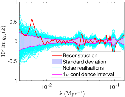
These non-parametric reconstructions suggest the presence of a feature at k0.006Mpc1similar-to𝑘0.006superscriptMpc1k\sim 0.006\,\mathrm{Mpc}^{-1} in Img22Imsubscript𝑔22\mathrm{Im}\,g_{22} with respect to both Bayesian and frequentist uncertainties. The dominant contributions to this feature are from the BipoSH coefficients ImA747422Imsubscriptsuperscript𝐴227474\mathrm{Im}\,A^{22}_{74~{}74} and ImA747622Imsubscriptsuperscript𝐴227476\mathrm{Im}\,A^{22}_{74~{}76} which are themselves bins of BipoSH coefficients in the multipole range 6090609060\leq\ell\leq 90. We now proceed to investigate the direction of this possible feature and its relation to known regions of interest.

One such is the hemispherical asymmetry, or dipole modulation of the CMB sky, first noted in ref.[16], which adds to the statistically isotropic CMB sky Tiso(𝐧^)subscript𝑇iso^𝐧T_{\mathrm{iso}}(\hat{\mathbf{n}}) a dipole A𝐩^𝐧^𝐴^𝐩^𝐧A\hat{\mathbf{p}}\cdot\hat{\mathbf{n}} resulting in a statistically anisotropic CMB sky

T(𝐧^)=Tiso(𝐧^)(1+A𝐩^𝐧^)𝑇^𝐧subscript𝑇iso^𝐧1𝐴^𝐩^𝐧\displaystyle T(\hat{\mathbf{n}})=T_{\mathrm{iso}}(\hat{\mathbf{n}})(1+A\hat{\mathbf{p}}\cdot\hat{\mathbf{n}}) (4.11)

where 𝐩^^𝐩\hat{\mathbf{p}} is the preferred direction and A𝐴A is the amplitude of the modulation. Proposed models [27, 28] invoke a large amplitude super-horizon perturbation of an additional field during inflation, or any mechanism that directionally modulates the optical depth of reionisation, scalar spectral index or tensor amplitude. Different analyses [12] have converged on there being a dipole modulation in the range 2642642\leq\ell\leq 64 at 3σsimilar-toabsent3𝜎\sim 3\sigma significance. We are sensitive to the latter half of this range. Higher multipole ranges are consistent with there being no dipole modulation at 2σ2𝜎2\sigma level [12], although if it persists beyond 64similar-to64\ell\sim 64, it is potentially observable in B mode polarisation [29]. The best-fit amplitude and direction from a BipoSH analysis of the PR2–2015 SMICA map in the quoted range give A=0.069±0.022𝐴plus-or-minus0.0690.022A=0.069\pm 0.022 and direction (l,b)=(228,18)±30𝑙𝑏plus-or-minussuperscript228superscript18superscript30(l,b)=(228^{\circ},-18^{\circ})\pm 30^{\circ}. Another region of interest is the well-known CMB dipole, which is interpreted as being a Doppler boost due to our motion relative to the ‘CMB rest frame’ in the direction (264,48)superscript264superscript48(264^{\circ},48^{\circ}) [12]. The Doppler boost itself induces a statistical anisotropy due to the aberration of light [30] and this too has a BipoSH description [31, 32].

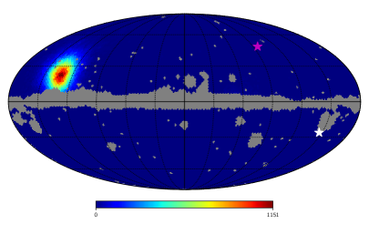
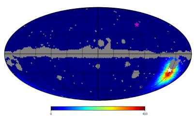
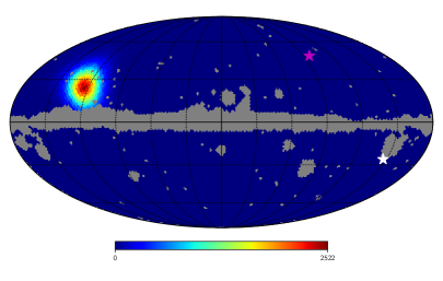
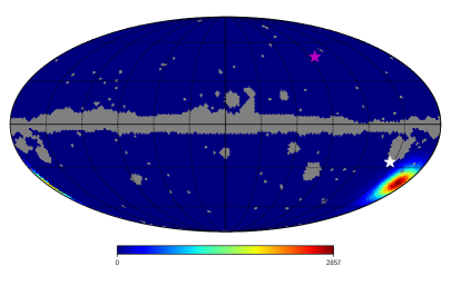
When fitting the quadrupole modulation of eq.(4.10) to the data over a limited wave number range, 0.005k/Mpc10.0080.005𝑘superscriptMpc10.0080.005\leq k/\mathrm{Mpc}^{-1}\leq 0.008, assuming just one direction 𝐧^1=𝐧^2subscript^𝐧1subscript^𝐧2\hat{\mathbf{n}}_{1}=\hat{\mathbf{n}}_{2} and a constant amplitude gAsubscript𝑔𝐴g_{A}, we find that the posterior probability distribution of the direction is bimodal. Histograms of the posterior distribution of the direction for both cases are shown in Fig. 15. Details of the directions are provided in Table 4 where angular distances to the CMB dipole and the hemispherical asymmetry (as determined in ref.[12]) are calculated.
Refer to caption
Refer to caption
Figure 15: Histograms of the posterior distribution of the direction 𝐧^^𝐧\hat{\mathbf{n}} for the case of a hot (109gA=0.75±0.22superscript109subscript𝑔𝐴plus-or-minus0.750.2210^{9}g_{A}=0.75\pm 0.22) constant quadrupole modulation (left panel) and a cold (109gA=0.82±0.21superscript109subscript𝑔𝐴plus-or-minus0.820.2110^{9}g_{A}=-0.82\pm 0.21) modulation (right panel) in the wave number range 0.005k/Mpc10.0080.005𝑘superscriptMpc10.0080.005\leq k/\mathrm{Mpc}^{-1}\leq 0.008. The SMICA mask (in grey) is superimposed for comparison. The magenta and white stars indicate the directions of the CMB dipole and the hemispherical asymmetry, respectively. The best-fit directions are (12814+14,259+11)subscriptsuperscriptsuperscript1281414subscriptsuperscriptsuperscript25119({128^{\circ}}^{+14}_{-14},{25^{\circ}}^{+11}_{-9}) for positive amplitude and (19114+15,4111+10)subscriptsuperscriptsuperscript1911514subscriptsuperscriptsuperscript411011({191^{\circ}}^{+15}_{-14},{-41^{\circ}}^{+10}_{-11}) for negative amplitude.
For k=0.005𝑘0.005k=0.005-0.008Mpc10.008superscriptMpc10.008\,\mathrm{Mpc}^{-1}: Angular distances to:
Amp. 109gAsuperscript109subscript𝑔𝐴10^{9}g_{A} Direction (l,b)𝑙𝑏(l,b) CMB dipole (264,48)superscript264superscript48(264^{\circ},48^{\circ}) Hemisph. asym. (213,26)superscript213superscript26(213^{\circ},-26^{\circ})
0.76±0.22plus-or-minus0.760.220.76\pm 0.22 (12814+14,259+11)subscriptsuperscriptsuperscript1281414subscriptsuperscriptsuperscript25119({128^{\circ}}^{+14}_{-14},{25^{\circ}}^{+11}_{-9}) 97superscript9797^{\circ} 97superscript9797^{\circ}
0.82±0.21plus-or-minus0.820.21-0.82\pm 0.21 (19114+15,4111+10)subscriptsuperscriptsuperscript1911514subscriptsuperscriptsuperscript411011({191^{\circ}}^{+15}_{-14},{-41^{\circ}}^{+10}_{-11}) 110superscript110110^{\circ} 24superscript2424^{\circ}
Table 4: Details of the two modes of the posterior distribution of the quadrupole modulation direction shown in Fig. 15. The first mode is for the case of a hot modulation. Angular distances to the directions of the CMB dipole and the hemispherical asymmetry are also indicated.

In the case of a ‘hot’ quadrupole modulation (gA>0subscript𝑔𝐴0g_{A}>0), the direction of the quadrupole modulation is, within the 10similar-toabsentsuperscript10\sim 10^{\circ} uncertainty, roughly perpendicular to the best-fit direction of hemispherical asymmetry. Within this uncertainty, it is also perpendicular to the best-fit direction of the CMB dipole. For the case of a ‘cold’ quadrupole modulation (gA<0subscript𝑔𝐴0g_{A}<0) the coincidences are less pronounced, however the direction is approximately aligned with that of the hemispherical asymmetry within the uncertainty. It is quite unexpected that the direction of the quadrupole modulation should be related to that of either the CMB dipole or the hemispherical asymmetry.

We will relegate the discussion of features and their statistical significance to the next section where all five components will be compressed to a single amplitude g2(k)subscript𝑔2𝑘g_{2}(k).

Refer to caption
Refer to caption
Refer to caption
Refer to caption
Refer to caption
Figure 16: Reconstruction (full red line) with credible intervals (purple band) and confidence intervals (cyan band) for λ=5000𝜆5000\lambda=5000.

4.4 The diagonal approximation

When forming an estimator for g2Msubscript𝑔2𝑀g_{2M} it is common for computational reasons to neglect in the Fisher matrix the off-diagonal elements of 𝐂1superscript𝐂1\mathbf{C}^{-1}, the inverse of the covariance Cm,mbmbmsubscript𝐶𝑚superscriptsuperscript𝑚delimited-⟨⟩subscript𝑏𝑚subscriptsuperscript𝑏superscriptsuperscript𝑚C_{\ell m,\ell^{\prime}m^{\prime}}\equiv\langle b_{\ell m}b^{\ast}_{\ell^{\prime}m^{\prime}}\rangle of the masked spherical harmonic coefficients [22, 12]. To enable comparison with these results we make here the equivalent approximation of truncating the BipoSH covariance matrix 𝚺𝚺\mathbf{\Sigma} to its diagonal alone. In this case we find no evidence of a constant quadrupole modulation nor one scaling with wave number as a power law. However when fitting a quadrupole modulation to the anomalous wave number range 0.0050.0050.005-0.008Mpc10.008superscriptMpc10.008\,\mathrm{Mpc}^{-1} in the diagonal approximation, the coincidences with the hemispherical asymmetry and CMB dipole are even more pronounced. The details are given in Appendix F.

5 Statistical significance of a quadrupole modulation

5.1 Power law quadrupole modulations

To test the statistical significance of power-law quadrupole modulation

g2M(k)=(4π)1/2g2M(k/k)q𝒫(k),subscript𝑔2𝑀𝑘superscript4𝜋12subscript𝑔2𝑀superscript𝑘subscript𝑘𝑞𝒫𝑘g_{2M}(k)=(4\pi)^{-1/2}g_{2M\star}(k/k_{\ast})^{q}\mathcal{P}(k), (5.1)

we calculate the overall amplitude

g2=15M|g2M|2subscript𝑔215subscript𝑀superscriptsubscript𝑔2𝑀2g_{2}=\sqrt{\frac{1}{5}\sum_{M}|g_{2M\star}|^{2}} (5.2)

for the components g^2Msubscript^𝑔2𝑀\hat{g}_{2M\star} that best fit the data and compare it with the estimates of g2subscript𝑔2g_{2} calculated from 104superscript10410^{4} realisations of noise modelled by the covariance matrix 𝚺𝚺\mathbf{\Sigma} derived from the FFP9 simulations. Each realisation is a set of BipoSH coefficients 𝐀2Msuperscript𝐀2𝑀\mathbf{A}^{2M} from which g2Msubscript𝑔2𝑀g_{2M\star} can be deduced using eq.(4.4). These are then used to compute g2subscript𝑔2g_{2}. The p-value is equal to the fraction of realisations with g2subscript𝑔2g_{2} greater than or equal to the value g^2subscript^𝑔2\hat{g}_{2} obtained from data and is shown in Table 5. The power-law cases 1q21𝑞2-1\leq q\leq 2 are unusual at the 2σsimilar-toabsent2𝜎\sim 2\sigma significance level, with q=0𝑞0q=0 the most significant at 2.16σ2.16𝜎2.16\sigma.

q𝑞q -2 -1 0 1 2
p-value 0.91 0.08 0.03 0.05 0.06
Table 5: P-value test of g2subscript𝑔2g_{2} (5.2) calculated for power law quadrupole modulations from data and compared with 104superscript10410^{4} noise realisations.

5.2 Non-parametric quadrupole modulations

We repeat the same procedure for the reconstructions g2M(k)subscript𝑔2𝑀𝑘g_{2M}(k) from data, calculating

g2(k)=15M|g2M(k)|2subscript𝑔2𝑘15subscript𝑀superscriptsubscript𝑔2𝑀𝑘2\displaystyle g_{2}(k)=\sqrt{\frac{1}{5}\sum_{M}|g_{2M}(k)|^{2}} (5.3)

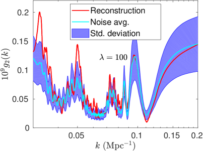
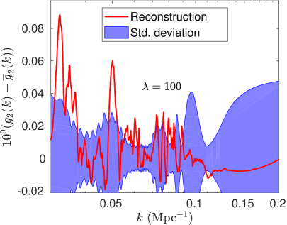
for the (λ=100𝜆100\lambda=100) reconstruction from data and for the (λ=100𝜆100\lambda=100) reconstructions from 104superscript10410^{4} realisations of noise only. The results are shown in Fig. 17, where on the right the mean of the noise realisations, g¯2(k)=N1j=Ng2,j(k)subscript¯𝑔2𝑘superscript𝑁1subscript𝑗𝑁subscript𝑔2𝑗𝑘\overline{g}_{2}(k)=N^{-1}\sum_{j=N}g_{2,j}(k) has been subtracted from g2(k)subscript𝑔2𝑘g_{2}(k). Using the noise realisations, a covariance matrix for g2(k)subscript𝑔2𝑘g_{2}(k) was constructed:

Σg2kk=1N1j=1N(g2,j(k)g¯2(k))(g2,j(k)g¯2(k)),subscriptΣsubscript𝑔2𝑘superscript𝑘1𝑁1superscriptsubscript𝑗1𝑁subscript𝑔2𝑗𝑘subscript¯𝑔2𝑘subscript𝑔2𝑗superscript𝑘subscript¯𝑔2superscript𝑘\displaystyle\Sigma_{g_{2}\,kk^{\prime}}=\frac{1}{N-1}\sum_{j=1}^{N}(g_{2,j}(k)-\overline{g}_{2}(k))(g_{2,j}(k^{\prime})-\overline{g}_{2}(k^{\prime})), (5.4)

the square root of whose diagonal values have been used as standard deviations in the plots of Fig. 17. The amplitude g2(k)subscript𝑔2𝑘g_{2}(k) suggests the presence of features at 0.006, 0.019, 0.033, 0.061, 0.0826, 0.086, and 0.096 Mpc1superscriptMpc1\mathrm{Mpc}^{-1}.

Refer to caption
Refer to caption
Figure 17: The left panel shows the amplitude g2(k)subscript𝑔2𝑘g_{2}(k) for the reconstruction from data (red line) and its mean (cyan line) and standard deviation (purple band) of g2(k)subscript𝑔2𝑘g_{2}(k) for the noise realisations. In the right panel, this mean g¯2(k)subscript¯𝑔2𝑘\overline{g}_{2}(k) has been subtracted from the g2(k)subscript𝑔2𝑘g_{2}(k) reconstructed from data.

However, a test of the global significance should be made. To do so, the constructed covariance matrix was inverted and used in a χ2superscript𝜒2\chi^{2} statistic:

Tg2(g2(k))=(𝐠2𝐠¯2)T𝚺g21(𝐠2𝐠¯2)subscript𝑇subscript𝑔2subscript𝑔2𝑘superscriptsubscript𝐠2subscript¯𝐠2𝑇subscriptsuperscript𝚺1subscript𝑔2subscript𝐠2subscript¯𝐠2\displaystyle T_{g_{2}}(g_{2}(k))=(\mathbf{g}_{2}-\overline{\mathbf{g}}_{2})^{T}\mathbf{\Sigma}^{-1}_{g_{2}}(\mathbf{g}_{2}-\overline{\mathbf{g}}_{2}) (5.5)

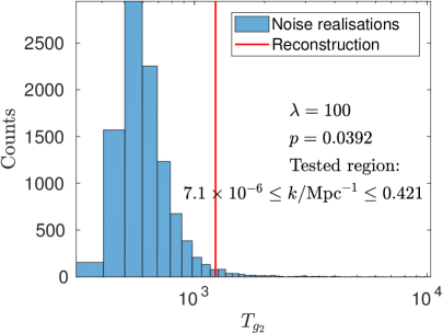
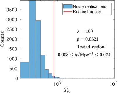
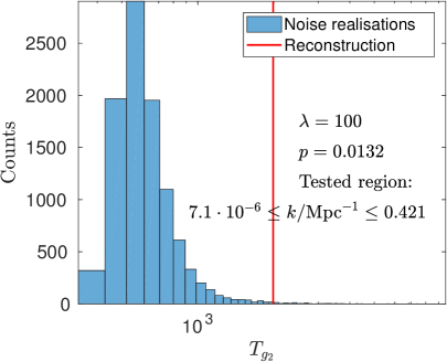
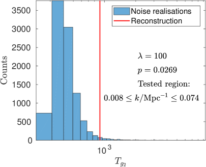
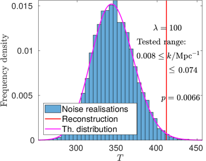
where the bold notation has been used to suppress the wave number indices. Strictly speaking, the covariance matrix is not invertible, so a pseudoinverse must be used instead. This statistic was calculated for the noise realisations as well as the reconstruction from data and a p-value was thus derived. The results are shown in Fig. 18 where the right panel shows the results of the p-value test for a region of wave numbers limited to 0.008k/Mpc10.0740.008𝑘superscriptMpc10.0740.008\leq k/\mathrm{Mpc}^{-1}\leq 0.074.

Refer to caption
Refer to caption
Figure 18: P-value test using Tg2subscript𝑇subscript𝑔2T_{g_{2}}. The distribution of Tg2subscript𝑇subscript𝑔2T_{g_{2}} for noise realisations and the value of Tg2subscript𝑇subscript𝑔2T_{g_{2}} for the reconstruction from data (red line). The right panel shows the same test, but for a more restricted range of wave numbers.

The p-values translate to 2.06σ2.06𝜎2.06\sigma and 2.14σ2.14𝜎2.14\sigma significance levels, respectively. These are quite marginal, however, we shall now argue that another test statistic should be adopted that is more sensitive and under better theoretical control. Though Tg2subscript𝑇subscript𝑔2T_{g_{2}} is based on the amplitude g2subscript𝑔2g_{2} which is rotationally invariant, it is not the case that all components g2Msubscript𝑔2𝑀g_{2M} are equally uncertain since the submatrices of the block matrix 𝚺𝚺\mathbf{\Sigma} corresponding to different components M𝑀M, are not equal to one another, and so equal statistical weight should not be given to all components. Since the statistic is based on the amplitude, it is insensitive to the direction. If a certain direction is systematically singled out across k𝑘k, but with a small amplitude, that will count no more than randomly oriented quadrupole modulations across k𝑘k. Also, we do not have good theoretical control over the test statistic Tg2subscript𝑇subscript𝑔2T_{g_{2}}. It can be seen in both panels of Fig. 18 that the possible values of Tg2subscript𝑇subscript𝑔2T_{g_{2}} for the noise realisations, although peaked around 500, still appear at values up to 10,000.

We shall now present a test statistic which addresses these issues. We construct a χ2superscript𝜒2\chi^{2} statistic using the frequentist covariance matrix

T(g2M)=𝐠T𝚺F1𝐠.𝑇subscript𝑔2𝑀superscript𝐠𝑇superscriptsubscript𝚺F1𝐠\displaystyle T(g_{2M})=\mathbf{g}^{T}{\mathbf{\Sigma}_{\mathrm{F}}}^{-1}\mathbf{g}. (5.6)

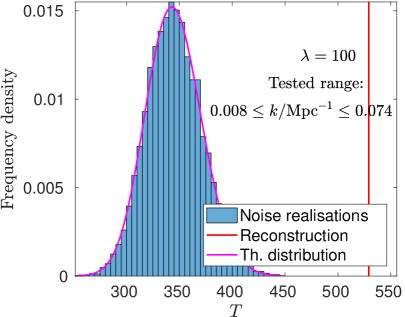
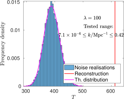
Strictly speaking, the inverse of the frequentist covariance matrix does not exist, but its pseudoinverse does. We have proven in Appendix D that (using the pseudoinverse) T(g2M)𝑇subscript𝑔2𝑀T(g_{2M}) is distributed according to a χ2superscript𝜒2\chi^{2} distribution with degrees of freedom equal to the rank of the pseudoinverse covariance matrix. This should equal the rank of the original covariance matrix of the data, which is 787878 per component of g2Msubscript𝑔2𝑀g_{2M} or 390 for all five (three real and two imaginary) components considered together. Therefore when using all the data the test statistic T𝑇T should have a χ2superscript𝜒2\chi^{2} distribution with 390 degrees of freedom.

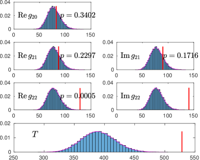
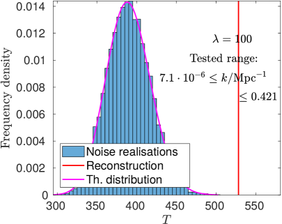
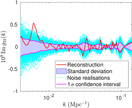
First we illustrate in the left panel of Fig. 19 that the frequentist covariance matrix corresponds to the standard deviation of reconstructed spectra of noise realisations. The standard deviation of the noise realisations of Img22Imsubscript𝑔22\mathrm{Im}\,g_{22} defining the purple band is exactly bounded by the magenta line which is the square root of the diagonal entries of 𝚺Fsubscript𝚺F\mathbf{\Sigma}_{\mathrm{F}} which give the 1σ1𝜎1\sigma confidence intervals. No noise realisations were found to have as extreme a value of T𝑇T. In fact, the theoretical distribution is able to tell us the answer: p=F390(613)3.7×10126.95σ𝑝subscript𝐹390613similar-to3.7superscript1012similar-to6.95𝜎p=F_{390}(613)\sim 3.7\times 10^{-12}\sim 6.95\sigma where F390subscript𝐹390F_{390} is the cumulative distribution function of χ3902superscriptsubscript𝜒3902\chi_{390}^{2}. By restricting the wave number range to 0.008k/Mpc10.0740.008𝑘superscriptMpc10.0740.008\leq k/\mathrm{Mpc}^{-1}\leq 0.074, we find that the reconstruction from data is made more likely. The results of the p-value tests are shown in Fig. 20. For the restricted range 0.008k/Mpc10.0740.008𝑘superscriptMpc10.0740.008\leq k/\mathrm{Mpc}^{-1}\leq 0.074, the p-value is F390(529)3.2×10⁶similar-tosubscript𝐹3905293.2superscript106F_{390}(529)\sim 3.2\times 10^{-6}, corresponding to 4.66σ4.66𝜎4.66\sigma significance. This illustrates clearly that even after cutting the data, the reconstructed spectrum is very unlikely to be a realisation of noise only.
Refer to caption
Figure 19: Noise realisations (thin cyan lines), their standard deviation (purple band) as well as the reconstruction from data (red line). The 1σ1𝜎1\sigma confidence interval (magenta lines) derived from the frequentist covariance matrix matches the standard deviation exactly.
Refer to caption
Refer to caption
Figure 20: P-value tests of T𝑇T for the full range of wave numbers (left panel) and a more limited range (right panel). The value of T𝑇T for the reconstruction from data is indicated with a red line.

When noise realisations are tested against the non-parametric reconstructions using a covariance matrix truncated to its diagonal entries, they are only marginally significant using the test statistic Tg2subscript𝑇subscript𝑔2T_{g_{2}} (2.5σ2.5𝜎2.5\sigma) but still rare (4.6σ4.6𝜎4.6\sigma) when using the directionally sensitive test statistic T𝑇T. For the restricted wave number range 0.008k/Mpc10.0740.008𝑘superscriptMpc10.0740.008\leq k/\mathrm{Mpc}^{-1}\leq 0.074 the significance drops to 2.2σ2.2𝜎2.2\sigma and 2.7σ2.7𝜎2.7\sigma for Tg2subscript𝑇subscript𝑔2T_{g_{2}} and T𝑇T, respectively.

6 Summary and Conclusions

We have described a method for reconstructing a direction- and scale-dependent modulation of the primordial power spectrum, using Tikhonov regularisation and the bipolar spherical harmonic representation. The BipoSH coefficients capture the statistical anisotropy of a CMB map and Tikhonov regularisation can then be used to infer the direction-dependent primordial power spectrum responsible. The uncertainties were estimated using the Planck FFP9 simulations and a simplified Gaussian likelihood was constructed. The method was then used on the PR2–2015 SMICA temperature map for the multipole range 30120030120030\leq\ell\leq 1200, binned with Δ=30Δ30\Delta\ell=30. The full covariance matrix of the binned BipoSH coefficients was used.

We find a 2.16σ2.16𝜎2.16\sigma indication of a constant quadrupole modulation, but less significance, 2σ2𝜎2\sigma, for the power law case. The best-fit directions are uncertain, but lie near the Galactic plane (l,b)=(8415+13,712+13)𝑙𝑏subscriptsuperscriptsuperscript841315subscriptsuperscriptsuperscript71312(l,b)=({84^{\circ}}^{+13}_{-15},{7^{\circ}}^{+13}_{-12}) for negative amplitudes, and orthogonal for positive amplitudes: b=1.9221+21𝑏subscriptsuperscriptsuperscript1.922121b={1.92^{\circ}}^{+21}_{-21} — suggesting contamination by Galactic foregrounds in the SMICA map. We find no evidence of either a constant or quadrupolar modulation only when we truncate the covariance matrix of the BipoSH coefficients to the diagonal.

However our non-parametric reconstruction suggests spectral features at wave number k/Mpc10.006,0.019,0.033,0.061,0.0826,0.086and0.096similar-to𝑘superscriptMpc10.0060.0190.0330.0610.08260.086and0.096k/\mathrm{Mpc}^{-1}\sim 0.006,0.019,0.033,0.061,0.0826,0.086~{}\mathrm{and}~{}0.096. The most prominent feature is at 0.006Mpc10.006superscriptMpc10.006\,\mathrm{Mpc}^{-1}, the dominant contribution to which comes from multipoles 6090609060\leq\ell\leq 90. When a constant quadrupole modulation is fitted to data in the wave number range 0.005k/Mpc10.0080.005𝑘superscriptMpc10.0080.005\leq k/\mathrm{Mpc}^{-1}\leq 0.008, the preferred direction of this modulation is related to the directions of the CMB dipole and hemispherical asymmetry. We find that a hot quadrupole modulation is perpendicular to both the CMB dipole and hemispherical asymmetry, while a cold quadrupole modulation is, within the uncertainties in direction, aligned with the hemispherical asymmetry. This is an unexpected result that merits further investigation.

In order to assess the global significance of the features, we construct two test statistics to evaluate reconstructions from data against reconstructions of noise only. With a test statistic sensitive only to the amplitude, we find the reconstruction from data to be unusual with 2.06σ2.06𝜎2.06\sigma significance for the full wave number range, and 2.14σ2.14𝜎2.14\sigma when we only consider intermediate wave numbers 0.008k/Mpc10.0740.008𝑘superscriptMpc10.0740.008\leq k/\mathrm{Mpc}^{-1}\leq 0.074. With the test statistic we believe to be more appropriate which is sensitive to a preferred direction as well, the significance increases to 6.95σ6.95𝜎6.95\sigma and 4.66σ4.66𝜎4.66\sigma, respectively, for the full and intermediate range of wave numbers.

Our method goes beyond previous work in allowing for non-parametric scale-dependence in a possible quadrupolar modulation and can be easily generalised to include higher order modulations as well. The binning in multipoles and restriction to 3030\ell\geq 30 can be avoided by constructing a non-Gaussian likelihood which makes full use of the Planck data and simulations. Other data sets such as polarisation, large-scale structure and future 21-cm line observations can also be incorporated. An immediate suggestion for future work would be to consider different Planck maps, and also consider different masks.

Acknowledgments

We thank Jeppe Trøst Nielsen for helpful suggestions and Sunny Vagnozzi, Sebastian von Hausegger, Hao Liu, Pavel Naselsky, Benjamin Wandelt, Guilhem Lavaux, Roya Mohayaee, Chris Pethick and Andrew Jackson for discussions. AD and SS were supported by the Danish National Research Foundation. SM acknowledges support from the Simons Foundation, the Labex ILP (ANR-10-LABX-63) part of the Idex SUPER, the Agence Nationale de la Recherche as part of the programme Investissements d’avenir (ANR-11-IDEX-0004-02), and hospitality at the Niels Bohr Institute where this work was initiated. SM also acknowledges the NERSC and Planck collaboration for providing the FFP simulations and auxiliary files.

References

Appendix A The general quadrupole

The resolution of

g(𝐤^𝐧^)2subscript𝑔superscript^𝐤^𝐧2g_{\ast}(\mathbf{\hat{k}}\cdot\mathbf{\hat{n}})^{2} (A.1)

not being the most general quadrupole modulation is simple: it is in fact

g(𝐤^𝐧^𝟏)(𝐤^𝐧^𝟐).subscript𝑔^𝐤subscript^𝐧1^𝐤subscript^𝐧2g_{\ast}(\mathbf{\hat{k}}\cdot\mathbf{\hat{n}_{1}})(\mathbf{\hat{k}}\cdot\mathbf{\hat{n}_{2}}). (A.2)

Clearly (A.1) is a special case of (A.2) when 𝐧^1=𝐧^2subscript^𝐧1subscript^𝐧2\hat{\mathbf{n}}_{1}=\hat{\mathbf{n}}_{2}. Moreover, (A.2) is the tensor product of two dipoles and therefore contains a quadrupole. Let us determine g2Msubscript𝑔2𝑀g_{2M} given the directions 𝐧^1subscript^𝐧1\hat{\mathbf{n}}_{1} and 𝐧^2subscript^𝐧2\hat{\mathbf{n}}_{2}. Let these be (θ1,ϕ1)subscript𝜃1subscriptitalic-ϕ1(\theta_{1},\phi_{1}) and (θ2,ϕ2)subscript𝜃2subscriptitalic-ϕ2(\theta_{2},\phi_{2}) while 𝐤^^𝐤\hat{\mathbf{k}} points in the direction (θ,ϕ)𝜃italic-ϕ(\theta,\phi). Then

g20subscript𝑔20\displaystyle g_{20} =gdΩ(𝐤^𝐧^𝟏)(𝐤^𝐧^𝟐)Y20(θ,ϕ)absentsubscript𝑔differential-dΩ^𝐤subscript^𝐧1^𝐤subscript^𝐧2superscriptsubscript𝑌20𝜃italic-ϕ\displaystyle=g_{\ast}\int\mathrm{d}\Omega\,(\mathbf{\hat{k}}\cdot\mathbf{\hat{n}_{1}})(\mathbf{\hat{k}}\cdot\mathbf{\hat{n}_{2}})Y_{20}^{\ast}(\theta,\phi)
=g14πdΩ(sin(θ)sin(θ1)cos(ϕϕ1)+cos(θ)cos(θ1))absentsubscript𝑔14𝜋differential-dΩ𝜃subscript𝜃1italic-ϕsubscriptitalic-ϕ1𝜃subscript𝜃1\displaystyle=g_{\ast}\frac{1}{\sqrt{4\pi}}\int\mathrm{d}\Omega\,(\sin(\theta)\sin(\theta_{1})\cos(\phi-\phi_{1})+\cos(\theta)\cos(\theta_{1}))
(sin(θ)sin(θ2)cos(ϕϕ2)+cos(θ)cos(θ2))Y20(θ,ϕ)𝜃subscript𝜃2italic-ϕsubscriptitalic-ϕ2𝜃subscript𝜃2superscriptsubscript𝑌20𝜃italic-ϕ\displaystyle\quad\quad\quad\quad(\sin(\theta)\sin(\theta_{2})\cos(\phi-\phi_{2})+\cos(\theta)\cos(\theta_{2}))Y_{20}^{\ast}(\theta,\phi) (A.3)
=g23π5(2cos(θ1)cos(θ2)cos(ϕ1ϕ2)sin(θ1)sin(θ2))absentsubscript𝑔23𝜋52subscript𝜃1subscript𝜃2subscriptitalic-ϕ1subscriptitalic-ϕ2subscript𝜃1subscript𝜃2\displaystyle=g_{\ast}\frac{2}{3}\sqrt{\frac{\pi}{5}}(2\cos(\theta_{1})\cos(\theta_{2})-\cos(\phi_{1}-\phi_{2})\sin(\theta_{1})\sin(\theta_{2})) (A.4)
g21subscript𝑔21\displaystyle g_{21} =gdΩ(𝐤^𝐧^𝟏)(𝐤^𝐧^𝟐)Y21(θ,ϕ)absentsubscript𝑔differential-dΩ^𝐤subscript^𝐧1^𝐤subscript^𝐧2superscriptsubscript𝑌21𝜃italic-ϕ\displaystyle=g_{\ast}\int\mathrm{d}\Omega\,(\mathbf{\hat{k}}\cdot\mathbf{\hat{n}_{1}})(\mathbf{\hat{k}}\cdot\mathbf{\hat{n}_{2}})Y_{21}^{\ast}(\theta,\phi) (A.5)
=g14πdΩ(sin(θ)sin(θ1)cos(ϕϕ1)+cos(θ)cos(θ1))absentsubscript𝑔14𝜋differential-dΩ𝜃subscript𝜃1italic-ϕsubscriptitalic-ϕ1𝜃subscript𝜃1\displaystyle=g_{\ast}\frac{1}{\sqrt{4\pi}}\int\mathrm{d}\Omega\,(\sin(\theta)\sin(\theta_{1})\cos(\phi-\phi_{1})+\cos(\theta)\cos(\theta_{1}))
(sin(θ)sin(θ2)cos(ϕϕ2)+cos(θ)cos(θ2))Y21(θ,ϕ)𝜃subscript𝜃2italic-ϕsubscriptitalic-ϕ2𝜃subscript𝜃2superscriptsubscript𝑌21𝜃italic-ϕ\displaystyle\quad\quad\quad\quad(\sin(\theta)\sin(\theta_{2})\cos(\phi-\phi_{2})+\cos(\theta)\cos(\theta_{2}))Y_{21}^{\ast}(\theta,\phi) (A.6)
=g2π15(exp(iϕ1)cos(θ2)sin(θ1)+exp(iϕ2)cos(θ1)sin(θ2))absentsubscript𝑔2𝜋15𝑖subscriptitalic-ϕ1subscript𝜃2subscript𝜃1𝑖subscriptitalic-ϕ2subscript𝜃1subscript𝜃2\displaystyle=-g_{\ast}\sqrt{\frac{2\pi}{15}}(\exp(-i\phi_{1})\cos(\theta_{2})\sin(\theta_{1})+\exp(-i\phi_{2})\cos(\theta_{1})\sin(\theta_{2})) (A.7)

and

g22subscript𝑔22\displaystyle g_{22} =gdΩ(𝐤^𝐧^𝟏)(𝐤^𝐧^𝟐)Y22(θ,ϕ)absentsubscript𝑔differential-dΩ^𝐤subscript^𝐧1^𝐤subscript^𝐧2superscriptsubscript𝑌22𝜃italic-ϕ\displaystyle=g_{\ast}\int\mathrm{d}\Omega\,(\mathbf{\hat{k}}\cdot\mathbf{\hat{n}_{1}})(\mathbf{\hat{k}}\cdot\mathbf{\hat{n}_{2}})Y_{22}^{\ast}(\theta,\phi) (A.8)
=g14πdΩ(sin(θ)sin(θ1)cos(ϕϕ1)+cos(θ)cos(θ1))absentsubscript𝑔14𝜋differential-dΩ𝜃subscript𝜃1italic-ϕsubscriptitalic-ϕ1𝜃subscript𝜃1\displaystyle=g_{\ast}\frac{1}{\sqrt{4\pi}}\int\mathrm{d}\Omega\,(\sin(\theta)\sin(\theta_{1})\cos(\phi-\phi_{1})+\cos(\theta)\cos(\theta_{1}))
(sin(θ)sin(θ2)cos(ϕϕ2)+cos(θ)cos(θ2))Y22(θ,ϕ)𝜃subscript𝜃2italic-ϕsubscriptitalic-ϕ2𝜃subscript𝜃2superscriptsubscript𝑌22𝜃italic-ϕ\displaystyle\quad\quad\quad\quad(\sin(\theta)\sin(\theta_{2})\cos(\phi-\phi_{2})+\cos(\theta)\cos(\theta_{2}))Y_{22}^{\ast}(\theta,\phi) (A.9)
=g2π15exp(i(ϕ1+ϕ2))sin(θ1)sin(θ2).absentsubscript𝑔2𝜋15𝑖subscriptitalic-ϕ1subscriptitalic-ϕ2subscript𝜃1subscript𝜃2\displaystyle=g_{\ast}\sqrt{\frac{2\pi}{15}}\exp(-i(\phi_{1}+\phi_{2}))\sin(\theta_{1})\sin(\theta_{2}). (A.10)

Appendix B Relating quadrupole modulations to BipoSH coefficients

We investigate in detail the relation between a given quadrupole modulation gLM(k)subscript𝑔𝐿𝑀𝑘g_{LM}(k) and the BipoSH coefficient ALMsubscriptsuperscript𝐴𝐿𝑀superscriptA^{LM}_{\ell\ell^{\prime}}. In linear theory, there is a simple relation between the temperature perturbation ΔT/T0Δ𝑇subscript𝑇0\Delta T/T_{0} in the direction 𝐧^^𝐧\mathbf{\hat{n}} at the position 𝐱𝐱\mathbf{x} at time t𝑡t and the curvature perturbation (𝐤)𝐤\mathcal{R}(\mathbf{k}), viz.

ΔTT0(𝐱,𝐧^,t)Δ𝑇subscript𝑇0𝐱^𝐧𝑡\displaystyle\frac{\Delta T}{T_{0}}(\mathbf{x},\mathbf{\hat{n}},t) =d3k(2π)3exp(i𝐤𝐱)Θ(𝐤,𝐧^,t)(𝐤),absentsuperscriptd3𝑘superscript2𝜋3𝑖𝐤𝐱Θ𝐤^𝐧𝑡𝐤\displaystyle=\int\frac{\mathrm{d}^{3}k}{\left(2\pi\right)^{3}}\exp(i\mathbf{k}\cdot\mathbf{x})\Theta(\mathbf{k},\mathbf{\hat{n}},t)\mathcal{R}(\mathbf{k}), (B.1)

where Θ(𝐤,𝐧,t)Θ𝐤𝐧𝑡\Theta(\mathbf{k},\mathbf{n},t) is the transfer function. Assuming that the cosmological evolution itself does not induce any anisotropy, the transfer function can depend only on 𝐤^𝐧^^𝐤^𝐧\mathbf{\hat{k}}\cdot\mathbf{\hat{n}} which takes values between -1 and 1. It can therefore be expressed in terms of Legendre polynomials P(𝐤^𝐧^)subscript𝑃^𝐤^𝐧P_{\ell}(\mathbf{\hat{k}}\cdot\mathbf{\hat{n}}) which are complete on the interval [1,1]11[-1,1], with coefficients ΘsubscriptΘ\Theta_{\ell}:

Θ(𝐤,𝐧^,t)Θ𝐤^𝐧𝑡\displaystyle\Theta(\mathbf{k},\mathbf{\hat{n}},t) =(i)(2+1)Θ(k,t)P(𝐤^𝐧^).absentsubscriptsuperscript𝑖21subscriptΘ𝑘𝑡subscript𝑃^𝐤^𝐧\displaystyle=\sum_{\ell}(-i)^{\ell}(2\ell+1)\Theta_{\ell}(k,t)P_{\ell}(\mathbf{\hat{k}}\cdot\mathbf{\hat{n}})\mathrm{.} (B.2)

The Legendre polynomials may be expressed as spherical harmonics:

P(𝐤^𝐧^)=4π2+1m=Ym(𝐤^)Ym(𝐧^),subscript𝑃^𝐤^𝐧4𝜋21superscriptsubscript𝑚subscript𝑌𝑚^𝐤subscriptsuperscript𝑌𝑚^𝐧\displaystyle P_{\ell}(\mathbf{\hat{k}}\cdot\mathbf{\hat{n}})=\frac{4\pi}{2\ell+1}\sum_{m=-\ell}^{\ell}Y_{\ell m}(\mathbf{\hat{k}})Y^{\ast}_{\ell m}(\mathbf{\hat{n}}), (B.3)

so that:

Θ(𝐤,𝐧^,t)Θ𝐤^𝐧𝑡\displaystyle\Theta(\mathbf{k},\mathbf{\hat{n}},t) =4πm(i)Θ(k,t)Ym(𝐤^)Ym(𝐧^).absent4𝜋subscript𝑚superscript𝑖subscriptΘ𝑘𝑡subscript𝑌𝑚^𝐤subscriptsuperscript𝑌𝑚^𝐧\displaystyle=4\pi\sum_{\ell m}(-i)^{\ell}\Theta_{\ell}(k,t)Y_{\ell m}(\mathbf{\hat{k}})Y^{\ast}_{\ell m}(\mathbf{\hat{n}})\mathrm{.} (B.4)

The central object is the angular correlation function

C(𝐧^,𝐧^)𝐶^𝐧superscript^𝐧\displaystyle C(\mathbf{\hat{n}},\mathbf{\hat{n}}^{\prime}) =ΔTT0(𝐱,𝐧^,t)ΔTT0(𝐱,𝐧^,t),absentdelimited-⟨⟩Δ𝑇subscript𝑇0𝐱^𝐧𝑡Δ𝑇subscript𝑇0𝐱superscript^𝐧𝑡\displaystyle=\Big{\langle}\frac{\Delta T}{T_{0}}(\mathbf{x},\mathbf{\hat{n}},t)\frac{\Delta T}{T_{0}}(\mathbf{x},\mathbf{\hat{n}}^{\prime},t)\Big{\rangle}, (B.5)

which can be re-expressed using (B.4):

C(𝐧^,𝐧^)𝐶^𝐧superscript^𝐧\displaystyle C(\mathbf{\hat{n}},\mathbf{\hat{n}}^{\prime}) =mm(4π)2(i)+Ym(𝐧^)Ym(𝐧^)absentsubscript𝑚subscriptsuperscriptsuperscript𝑚superscript4𝜋2superscript𝑖superscriptsubscript𝑌𝑚^𝐧subscript𝑌superscriptsuperscript𝑚superscript^𝐧\displaystyle=\sum_{\ell m}\sum_{\ell^{\prime}m^{\prime}}(4\pi)^{2}(-i)^{\ell+\ell^{\prime}}Y_{\ell m}(\mathbf{\hat{n}})Y_{\ell^{\prime}m^{\prime}}(\mathbf{\hat{n}}^{\prime})
d3k(2π)3d3k(2π)3ei(𝐤+𝐤)𝐱Θ(k,t)Θ(k,t)Ym(𝐤^)Ym(𝐤^)(𝐤)(𝐤).superscriptd3𝑘superscript2𝜋3superscriptd3superscript𝑘superscript2𝜋3superscripte𝑖𝐤superscript𝐤𝐱subscriptΘ𝑘𝑡subscriptΘsuperscriptsuperscript𝑘𝑡subscriptsuperscript𝑌𝑚^𝐤superscriptsubscript𝑌superscriptsuperscript𝑚superscript^𝐤delimited-⟨⟩𝐤superscript𝐤\displaystyle\quad\int\frac{\mathrm{d}^{3}k}{(2\pi)^{3}}\int\frac{\mathrm{d}^{3}k^{\prime}}{(2\pi)^{3}}\mathrm{e}^{i(\mathbf{k}+\mathbf{k^{\prime}})\cdot\mathbf{x}}\Theta_{\ell}(k,t)\Theta_{\ell^{\prime}}(k^{\prime},t)Y^{\ast}_{\ell m}(\mathbf{\hat{k}})Y_{\ell^{\prime}m^{\prime}}^{\ast}(\mathbf{\hat{k}}^{\prime})\langle\mathcal{R}(\mathbf{k})\mathcal{R}(\mathbf{k}^{\prime})\rangle. (B.6)

Now, we know that

(𝐤)(𝐤)delimited-⟨⟩𝐤superscript𝐤\displaystyle\langle\mathcal{R}(\mathbf{k})\mathcal{R}(\mathbf{k}^{\prime})\rangle =(2π)3δ(3)(𝐤+𝐤)P(𝐤)absentsuperscript2𝜋3superscript𝛿3𝐤superscript𝐤𝑃𝐤\displaystyle=(2\pi)^{3}\delta^{(3)}(\mathbf{k}+\mathbf{k}^{\prime})P(\mathbf{k}) (B.7)
=(2π)3δ(3)(𝐤+𝐤)2π2k3𝒫(𝐤)absentsuperscript2𝜋3superscript𝛿3𝐤superscript𝐤2superscript𝜋2superscript𝑘3𝒫𝐤\displaystyle=(2\pi)^{3}\delta^{(3)}(\mathbf{k}+\mathbf{k}^{\prime})\frac{2\pi^{2}}{k^{3}}\mathcal{P}(\mathbf{k}) (B.8)
=(2π)3δ(3)(𝐤+𝐤)2π2k34πLMgLM(k)YLM(𝐤^),absentsuperscript2𝜋3superscript𝛿3𝐤superscript𝐤2superscript𝜋2superscript𝑘34𝜋subscript𝐿𝑀subscript𝑔𝐿𝑀𝑘subscript𝑌𝐿𝑀^𝐤\displaystyle=(2\pi)^{3}\delta^{(3)}(\mathbf{k}+\mathbf{k}^{\prime})\frac{2\pi^{2}}{k^{3}}\sqrt{4\pi}\sum_{LM}g_{LM}(k)Y_{LM}(\mathbf{\hat{k}}), (B.9)

so, replacing (𝐤)(𝐤)delimited-⟨⟩𝐤superscript𝐤\langle\mathcal{R}(\mathbf{k})\mathcal{R}(\mathbf{k}^{\prime})\rangle, we get

C(𝐧^,𝐧^)𝐶^𝐧superscript^𝐧\displaystyle C(\mathbf{\hat{n}},\mathbf{\hat{n}}^{\prime}) =4πmm(4π)2(i)+Ym(𝐧^)Ym(𝐧^)d3k(2π)3d3k(2π)3ei(𝐤+𝐤)𝐱absent4𝜋subscript𝑚subscriptsuperscriptsuperscript𝑚superscript4𝜋2superscript𝑖superscriptsubscript𝑌𝑚^𝐧subscript𝑌superscriptsuperscript𝑚superscript^𝐧superscriptd3𝑘superscript2𝜋3superscriptd3superscript𝑘superscript2𝜋3superscripte𝑖𝐤superscript𝐤𝐱\displaystyle=\sqrt{4\pi}\sum_{\ell m}\sum_{\ell^{\prime}m^{\prime}}(4\pi)^{2}(-i)^{\ell+\ell^{\prime}}Y_{\ell m}(\mathbf{\hat{n}})Y_{\ell^{\prime}m^{\prime}}(\mathbf{\hat{n}}^{\prime})\int\frac{\mathrm{d}^{3}k}{(2\pi)^{3}}\int\frac{\mathrm{d}^{3}k^{\prime}}{(2\pi)^{3}}\mathrm{e}^{i(\mathbf{k}+\mathbf{k^{\prime}})\cdot\mathbf{x}}
Θ(k,t)Θ(k,t)Ym(𝐤^)Ym(𝐤^)(2π)3δ(3)(𝐤+𝐤)2π2k3LMgLM(k)YLM(𝐤^).subscriptΘ𝑘𝑡subscriptΘsuperscriptsuperscript𝑘𝑡subscriptsuperscript𝑌𝑚^𝐤superscriptsubscript𝑌superscriptsuperscript𝑚superscript^𝐤superscript2𝜋3superscript𝛿3𝐤superscript𝐤2superscript𝜋2superscript𝑘3subscript𝐿𝑀subscript𝑔𝐿𝑀𝑘subscript𝑌𝐿𝑀^𝐤\displaystyle\quad\Theta_{\ell}(k,t)\Theta_{\ell^{\prime}}(k^{\prime},t)Y^{\ast}_{\ell m}(\mathbf{\hat{k}})Y_{\ell^{\prime}m^{\prime}}^{\ast}(\mathbf{\hat{k}^{\prime}})(2\pi)^{3}\delta^{(3)}(\mathbf{k}+\mathbf{k}^{\prime})\frac{2\pi^{2}}{k^{3}}\sum_{LM}g_{LM}(k)Y_{LM}(\mathbf{\hat{k}})\mathrm{.} (B.10)

The 3-dimensional integral over 𝐤superscript𝐤\mathbf{k}^{\prime} is trivial due to the δ𝛿\delta function and the 3-dimensional integral over 𝐤𝐤\mathbf{k} is split into a radial part and an angular part:

C(𝐧^,𝐧^)𝐶^𝐧superscript^𝐧\displaystyle C(\mathbf{\hat{n}},\mathbf{\hat{n}}^{\prime}) =4πLMmm(4π)2(i)+1(2π)3Ym(𝐧^)Ym(𝐧^)absent4𝜋subscript𝐿𝑀subscript𝑚subscriptsuperscriptsuperscript𝑚superscript4𝜋2superscript𝑖superscript1superscript2𝜋3subscript𝑌𝑚^𝐧subscript𝑌superscriptsuperscript𝑚superscript^𝐧\displaystyle=\sqrt{4\pi}\sum_{LM}\sum_{\ell m}\sum_{\ell^{\prime}m^{\prime}}(4\pi)^{2}(-i)^{\ell+\ell^{\prime}}\frac{1}{(2\pi)^{3}}Y_{\ell m}(\mathbf{\hat{n}})Y_{\ell^{\prime}m^{\prime}}(\mathbf{\hat{n}}^{\prime})
0dkk22π2k3gLM(k)Θ(k,t)Θ(k,t)d𝐤^YLM(𝐤^)Ym(𝐤^)Ym(𝐤^).superscriptsubscript0differential-d𝑘superscript𝑘22superscript𝜋2superscript𝑘3subscript𝑔𝐿𝑀𝑘subscriptΘ𝑘𝑡subscriptΘsuperscript𝑘𝑡differential-d^𝐤subscript𝑌𝐿𝑀^𝐤subscriptsuperscript𝑌𝑚^𝐤superscriptsubscript𝑌superscriptsuperscript𝑚^𝐤\displaystyle\quad\int_{0}^{\infty}\mathrm{d}k\,k^{2}\frac{2\pi^{2}}{k^{3}}g_{LM}(k)\Theta_{\ell}(k,t)\Theta_{\ell^{\prime}}(k,t)\int\mathrm{d}\mathbf{\hat{k}}\,Y_{LM}(\mathbf{\hat{k}})Y^{\ast}_{\ell m}(\mathbf{\hat{k}})Y_{\ell^{\prime}m^{\prime}}^{\ast}(-\mathbf{\hat{k}}). (B.11)

Using Ym(𝐤^)=(1)Ym(𝐤^)=(i)2Ym(𝐤^)subscript𝑌superscriptsuperscript𝑚^𝐤superscript1superscriptsubscript𝑌superscriptsuperscript𝑚^𝐤superscript𝑖2superscriptsubscript𝑌superscriptsuperscript𝑚^𝐤Y_{\ell^{\prime}m^{\prime}}(-\mathbf{\hat{k}})=(-1)^{\ell^{\prime}}Y_{\ell^{\prime}m^{\prime}}(\mathbf{\hat{k}})=(-i)^{2\ell^{\prime}}Y_{\ell^{\prime}m^{\prime}}(\mathbf{\hat{k}}) we get

C(𝐧,𝐧)𝐶𝐧superscript𝐧\displaystyle C(\mathbf{n},\mathbf{n}^{\prime}) =4πLMmm(4π)2(i)+1(2π)3Ym(𝐧^)Ym(𝐧^)absent4𝜋subscript𝐿𝑀subscript𝑚subscriptsuperscriptsuperscript𝑚superscript4𝜋2superscript𝑖superscript1superscript2𝜋3subscript𝑌𝑚^𝐧subscript𝑌superscriptsuperscript𝑚superscript^𝐧\displaystyle=\sqrt{4\pi}\sum_{LM}\sum_{\ell m}\sum_{\ell^{\prime}m^{\prime}}(4\pi)^{2}(-i)^{\ell+\ell^{\prime}}\frac{1}{(2\pi)^{3}}Y_{\ell m}(\mathbf{\hat{n}})Y_{\ell^{\prime}m^{\prime}}(\mathbf{\hat{n}}^{\prime})
0dkk22π2k3gLM(k)Θ(k,t)Θ(k,t)d𝐤^YLM(𝐤^)Ym(𝐤^)(i)2Ym(𝐤^),superscriptsubscript0differential-d𝑘superscript𝑘22superscript𝜋2superscript𝑘3subscript𝑔𝐿𝑀𝑘subscriptΘ𝑘𝑡subscriptΘsuperscript𝑘𝑡differential-d^𝐤subscript𝑌𝐿𝑀^𝐤subscriptsuperscript𝑌𝑚^𝐤superscript𝑖2superscriptsuperscriptsubscript𝑌superscriptsuperscript𝑚^𝐤\displaystyle\quad\int_{0}^{\infty}\mathrm{d}k\,k^{2}\frac{2\pi^{2}}{k^{3}}g_{LM}(k)\Theta_{\ell}(k,t)\Theta_{\ell^{\prime}}(k,t)\int\mathrm{d}\mathbf{\hat{k}}\,Y_{LM}(\mathbf{\hat{k}})Y^{\ast}_{\ell m}(\mathbf{\hat{k}})(-i)^{-2\ell^{\prime}}Y_{\ell^{\prime}m^{\prime}}^{\ast}(\mathbf{\hat{k}}), (B.12)

where the numerical factors may be combined, and factors shuffled, to write:

C(𝐧^,𝐧^)𝐶^𝐧superscript^𝐧\displaystyle C(\mathbf{\hat{n}},\mathbf{\hat{n}^{\prime}}) =4πLMmm(4π)(i)Ym(𝐧^)Ym(𝐧^)absent4𝜋subscript𝐿𝑀subscript𝑚subscriptsuperscriptsuperscript𝑚4𝜋superscript𝑖superscriptsubscript𝑌𝑚^𝐧subscript𝑌superscriptsuperscript𝑚superscript^𝐧\displaystyle=\sqrt{4\pi}\sum_{LM}\sum_{\ell m}\sum_{\ell^{\prime}m^{\prime}}(4\pi)(-i)^{\ell-\ell^{\prime}}Y_{\ell m}(\mathbf{\hat{n}})Y_{\ell^{\prime}m^{\prime}}(\mathbf{\hat{n}}^{\prime})
0dkkgLM(k)Θ(k,t)Θ(k,t)d𝐤^YLM(𝐤^)Ym(𝐤^)Ym(𝐤^).superscriptsubscript0d𝑘𝑘subscript𝑔𝐿𝑀𝑘subscriptΘ𝑘𝑡subscriptΘsuperscript𝑘𝑡differential-d^𝐤subscript𝑌𝐿𝑀^𝐤subscriptsuperscript𝑌𝑚^𝐤superscriptsubscript𝑌superscriptsuperscript𝑚^𝐤\displaystyle\quad\int_{0}^{\infty}\frac{\mathrm{d}k}{k}g_{LM}(k)\Theta_{\ell}(k,t)\Theta_{\ell^{\prime}}(k,t)\int\mathrm{d}\mathbf{\hat{k}}\,Y_{LM}(\mathbf{\hat{k}})Y^{\ast}_{\ell m}(\mathbf{\hat{k}})Y_{\ell^{\prime}m^{\prime}}^{\ast}(\mathbf{\hat{k}}). (B.13)

Now

d𝐤^YLM(𝐤^)Ym(𝐤^)Ym(𝐤^)=(1)m(2+1)(2+1)4π(2L+1)C00L0CmmLM,differential-d^𝐤subscript𝑌𝐿𝑀^𝐤subscriptsuperscript𝑌𝑚^𝐤superscriptsubscript𝑌superscriptsuperscript𝑚^𝐤superscript1superscript𝑚212superscript14𝜋2𝐿1subscriptsuperscript𝐶𝐿00superscript0subscriptsuperscript𝐶𝐿𝑀𝑚superscriptsuperscript𝑚\displaystyle\int\mathrm{d}\mathbf{\hat{k}}\,Y_{LM}(\mathbf{\hat{k}})Y^{\ast}_{\ell m}(\mathbf{\hat{k}})Y_{\ell^{\prime}m^{\prime}}^{\ast}(\mathbf{\hat{k}})=(-1)^{m^{\prime}}\sqrt{\frac{(2\ell+1)(2\ell^{\prime}+1)}{4\pi(2L+1)}}C^{L0}_{\ell 0\ell^{\prime}0}C^{LM}_{\ell m\ell^{\prime}-m^{\prime}}, (B.14)

and the factors of 4π4𝜋\sqrt{4\pi} cancel, yielding

C(𝐧^,𝐧^)𝐶^𝐧superscript^𝐧\displaystyle C(\mathbf{\hat{n}},\mathbf{\hat{n}^{\prime}}) =LMmmYm(𝐧^)Ym(𝐧^)CmmLM(1)mC00L0(2+1)(2+1)(2L+1)absentsubscript𝐿𝑀subscriptsuperscriptsubscript𝑚superscript𝑚subscript𝑌𝑚^𝐧subscript𝑌superscriptsuperscript𝑚superscript^𝐧subscriptsuperscript𝐶𝐿𝑀𝑚superscriptsuperscript𝑚superscript1superscript𝑚subscriptsuperscript𝐶𝐿00superscript0212superscript12𝐿1\displaystyle=\sum_{LM}\sum_{\ell\ell^{\prime}}\sum_{mm^{\prime}}Y_{\ell m}(\mathbf{\hat{n}})Y_{\ell^{\prime}m^{\prime}}(\mathbf{\hat{n}}^{\prime})C^{LM}_{\ell m\ell^{\prime}-m^{\prime}}(-1)^{m^{\prime}}C^{L0}_{\ell 0\ell^{\prime}0}\sqrt{\frac{(2\ell+1)(2\ell^{\prime}+1)}{(2L+1)}}
×[4π(i)0dlogkgLM(k)Θ(k,t)Θ(k,t)].absentdelimited-[]4𝜋superscript𝑖superscriptsuperscriptsubscript0d𝑘subscript𝑔𝐿𝑀𝑘subscriptΘ𝑘𝑡subscriptΘsuperscript𝑘𝑡\displaystyle\quad\times\left[4\pi(-i)^{\ell-\ell^{\prime}}\int_{0}^{\infty}\mathrm{d}\log k\,g_{LM}(k)\Theta_{\ell}(k,t)\Theta_{\ell^{\prime}}(k,t)\right]\mathrm{.} (B.15)

The square brackets isolate the BipoSH coefficients from the (WMAP normalised) basis functions and the expression matches eq.(2.8) after identifying ΘΘ\Theta with ΔΔ\Delta.

Appendix C Other choices of 𝝀𝝀\lambda

We present here the reconstructions for other values of the regularisation parameter λ𝜆\lambda. The results for λ=500𝜆500\lambda=500 are shown in Fig. 21. Note the feature at k0.006Mpc1similar-to𝑘0.006superscriptMpc1k\sim 0.006\,\mathrm{Mpc}^{-1} which persists when λ𝜆\lambda is increased to 1000 as shown in Fig. 22. The reconstructions for λ=10000𝜆10000\lambda=10000 are shown in Fig. 23. The quadrupole modulation g2Msubscript𝑔2𝑀g_{2M} at k0.006Mpc1similar-to𝑘0.006superscriptMpc1k\sim 0.006\,\mathrm{Mpc}^{-1} is tabulated in Table 6.
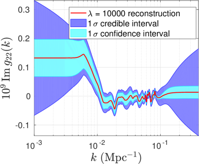
M𝑀M 109Reg2Msuperscript109Resubscript𝑔2𝑀10^{9}\,\mathrm{Re}\,{g}_{2M} 109Img2Msuperscript109Imsubscript𝑔2𝑀10^{9}\,\mathrm{Im}\,{g}_{2M}
00 0.23±0.16plus-or-minus0.230.16-0.23\pm 0.16
111 0.38±0.13plus-or-minus0.380.130.38\pm 0.13 0.17±0.13plus-or-minus0.170.130.17\pm 0.13
222 0.20±0.14plus-or-minus0.200.14-0.20\pm 0.14 0.50±0.14plus-or-minus0.500.140.50\pm 0.14
Table 6: The quadrupole modulation at k0.006Mpc1similar-to𝑘0.006superscriptMpc1k\sim 0.006\,\mathrm{Mpc}^{-1} with frequentist errors, from the reconstruction with λ=100𝜆100\lambda=100.
Refer to caption
Refer to caption
Refer to caption
Refer to caption
Refer to caption
Figure 21: Reconstructed quadrupole modulation (full red line) with 1σ1𝜎1\sigma credible intervals (purple) and 1σ1𝜎1\sigma confidence intervals (cyan) for λ=500𝜆500\lambda=500. Note the feature in Img22Imsubscript𝑔22\mathrm{Im}\,g_{22} at k0.006Mpc1similar-to𝑘0.006superscriptMpc1k\sim 0.006\,\mathrm{Mpc}^{-1}.
Refer to caption
Refer to caption
Refer to caption
Refer to caption
Refer to caption
Figure 22: Reconstruction for λ=1000𝜆1000\lambda=1000.
Refer to caption
Refer to caption
Refer to caption
Refer to caption
Refer to caption
Figure 23: Reconstruction for λ=10000𝜆10000\lambda=10000.

Appendix D The distribution of 𝑻𝑻T

It is shown below that the test statistic in eq.(5.6):

T(g2M,λ)𝑇subscript𝑔2𝑀𝜆\displaystyle T(g_{2M},\lambda) =𝐠T𝚺F+(𝐠),absentsuperscript𝐠𝑇superscriptsubscript𝚺F𝐠\displaystyle=\mathbf{g}^{T}\mathbf{\Sigma}_{\mathrm{F}}^{+}(\mathbf{g}), (D.1)

follows a χ2superscript𝜒2\chi^{2} distribution with degrees of freedom equal to the rank of the pseudoinverse of the covariance matrix.

Let the N×N𝑁𝑁N\times N covariance matrix 𝚺Fsubscript𝚺F\mathbf{\Sigma}_{\mathrm{F}} be diagonalised as

𝚺F=𝐔𝐃𝐔T,subscript𝚺Fsuperscript𝐔𝐃𝐔𝑇\mathbf{\Sigma}_{\mathrm{F}}=\mathbf{U}\mathbf{D}\mathbf{U}^{T}, (D.2)

where 𝐃𝐃\mathbf{D} is a diagonal matrix. The pseudoinverse of the covariance matrix then reads

𝚺F+=𝐔𝐃~𝐔Tsuperscriptsubscript𝚺F𝐔~𝐃superscript𝐔𝑇\mathbf{\Sigma}_{\mathrm{F}}^{+}=\mathbf{U}\mathbf{\tilde{D}}\mathbf{U}^{T} (D.3)

where 𝐃~~𝐃\mathbf{\tilde{D}} is the matrix that results from replacing the non-zero diagonal elements by their reciprocal. Further decompose 𝐃~~𝐃\mathbf{\tilde{D}} into 𝐃~=𝐃~1/2(𝐃~1/2)T~𝐃superscript~𝐃12superscriptsuperscript~𝐃12𝑇\mathbf{\tilde{D}}=\mathbf{\tilde{D}}^{1/2}(\mathbf{\tilde{D}}^{1/2})^{T} such that

𝚺F+=𝐔𝐃~1/2(𝐃~1/2)T𝐔T,superscriptsubscript𝚺F𝐔superscript~𝐃12superscriptsuperscript~𝐃12𝑇superscript𝐔𝑇\mathbf{\Sigma}_{\mathrm{F}}^{+}=\mathbf{U}\mathbf{\tilde{D}}^{1/2}(\mathbf{\tilde{D}}^{1/2})^{T}\mathbf{U}^{T}, (D.4)

where 𝐃~1/2superscript~𝐃12\mathbf{\tilde{D}}^{1/2} is a matrix with the diagonal elements equal to the square root of those of 𝐃𝐃\mathbf{D} and with the zero columns removed. There are Nrank(𝚺F+)𝑁ranksubscriptsuperscript𝚺FN-\mathrm{rank}(\mathbf{\Sigma}^{+}_{\mathrm{F}}) such columns. Transform to new variables

𝐲=(𝐃~1/2)T𝐔T𝐠,𝐲superscriptsuperscript~𝐃12𝑇superscript𝐔𝑇𝐠\mathbf{y}=(\mathbf{\tilde{D}}^{1/2})^{T}\mathbf{U}^{T}\mathbf{g}, (D.5)

which is a variable of dimension rank(𝚺F+)ranksubscriptsuperscript𝚺F\mathrm{rank}(\mathbf{\Sigma}^{+}_{\mathrm{F}}) so the test statistic becomes

T(y2M,λ)=𝐲T𝐲.𝑇subscript𝑦2𝑀𝜆superscript𝐲𝑇𝐲.T(y_{2M},\lambda)=\mathbf{y}^{T}\mathbf{y}\textrm{.} (D.6)

If each component of 𝐲𝐲\mathbf{y} is distributed according to a univariate Gaussian distribution, then T𝑇T, which consists of a sum of squares of such variables, has a χ2superscript𝜒2\chi^{2} distribution with degrees of freedom equal to the number of variables, namely rank(𝚺F+)ranksuperscriptsubscript𝚺F\mathrm{rank}(\mathbf{\Sigma}_{\mathrm{F}}^{+}). This is indeed the case, as the covariance matrix equals the identity matrix

𝐲𝐲Tdelimited-⟨⟩superscript𝐲𝐲𝑇\displaystyle\langle\mathbf{y}\mathbf{y}^{T}\rangle =(𝐃~1/2)T𝐔T𝐠𝐠T𝐔𝐃~1/2,absentdelimited-⟨⟩superscriptsuperscript~𝐃12𝑇superscript𝐔𝑇superscript𝐠𝐠𝑇𝐔superscript~𝐃12,\displaystyle=\langle(\mathbf{\tilde{D}}^{1/2})^{T}\mathbf{U}^{T}\mathbf{g}\mathbf{g}^{T}\mathbf{U}\mathbf{\tilde{D}}^{1/2}\rangle\textrm{,} (D.7)

and the expectation values may be taken to exclude the constant parts so that

𝐲𝐲Tdelimited-⟨⟩superscript𝐲𝐲𝑇\displaystyle\langle\mathbf{y}\mathbf{y}^{T}\rangle =(𝐃~1/2)T𝐔T𝐠𝐠T𝐔𝐃~1/2,absentsuperscriptsuperscript~𝐃12𝑇superscript𝐔𝑇delimited-⟨⟩superscript𝐠𝐠𝑇𝐔superscript~𝐃12\displaystyle=(\mathbf{\tilde{D}}^{1/2})^{T}\mathbf{U}^{T}\langle\mathbf{g}\mathbf{g}^{T}\rangle\mathbf{U}\mathbf{\tilde{D}}^{1/2}, (D.8)

and evaluated to give the frequentist covariance matrix 𝚺Fsubscript𝚺F\mathbf{\Sigma}_{\mathrm{F}}:

𝐲(𝐲)Tdelimited-⟨⟩𝐲superscript𝐲𝑇\displaystyle\langle\mathbf{y}(\mathbf{y})^{T}\rangle =(𝐃~1/2)T𝐔T𝚺F𝐔𝐃~1/2.absentsuperscriptsuperscript~𝐃12𝑇superscript𝐔𝑇subscript𝚺F𝐔superscript~𝐃12\displaystyle=(\mathbf{\tilde{D}}^{1/2})^{T}\mathbf{U}^{T}\mathbf{\Sigma}_{\mathrm{F}}\mathbf{U}\mathbf{\tilde{D}}^{1/2}. (D.9)

Expressing this in the diagonalised form (D.2) and reordering we get

𝐲𝐲Tdelimited-⟨⟩superscript𝐲𝐲𝑇\displaystyle\langle\mathbf{y}\mathbf{y}^{T}\rangle =(𝐃~1/2)T𝐔T(𝐔𝐃𝐔T)𝐔𝐃~1/2absentsuperscriptsuperscript~𝐃12𝑇superscript𝐔𝑇superscript𝐔𝐃𝐔𝑇𝐔superscript~𝐃12\displaystyle=(\mathbf{\tilde{D}}^{1/2})^{T}\mathbf{U}^{T}(\mathbf{U}\mathbf{D}\mathbf{U}^{T})\mathbf{U}\mathbf{\tilde{D}}^{1/2} (D.10)
=(𝐃~1/2)T(𝐔T𝐔)𝐃(𝐔T𝐔)𝐃~1/2=(𝐃~1/2)T𝐃𝐃~1/2=𝐈,absentsuperscriptsuperscript~𝐃12𝑇superscript𝐔𝑇𝐔𝐃superscript𝐔𝑇𝐔superscript~𝐃12superscriptsuperscript~𝐃12𝑇𝐃superscript~𝐃12𝐈\displaystyle=(\mathbf{\tilde{D}}^{1/2})^{T}(\mathbf{U}^{T}\mathbf{U})\mathbf{D}(\mathbf{U}^{T}\mathbf{U})\mathbf{\tilde{D}}^{1/2}=(\mathbf{\tilde{D}}^{1/2})^{T}\mathbf{D}\mathbf{\tilde{D}}^{1/2}=\mathbf{I}, (D.11)

since 𝐔T𝐔=𝐈superscript𝐔𝑇𝐔𝐈\mathbf{U}^{T}\mathbf{U}=\mathbf{I} (𝐔𝐔\mathbf{U} is orthogonal as 𝚺Fsubscript𝚺F\mathbf{\Sigma}_{\mathrm{F}}, the matrix being diagonalised, is symmetric).

Appendix E The Anderson-Darling test

The Anderson-Darling test [24] checks if a particular sample is likely to have come from a given distribution. Consider a sample x1,x2,,xnsubscript𝑥1subscript𝑥2subscript𝑥𝑛x_{1},x_{2},\ldots,x_{n} of a stochastic variable X𝑋X. When this is sorted in ascending order x(1),x(2),,x(n)subscript𝑥1subscript𝑥2subscript𝑥𝑛x_{(1)},x_{(2)},\ldots,x_{(n)}, the empirical distribution function Fn(x)subscript𝐹𝑛𝑥F_{n}(x) can be constructed as the fraction of the sample that has values less than or equal to x𝑥x. In asking if a sample is likely to come from a probability distribution P(x,𝜽)𝑃𝑥𝜽P(x,\boldsymbol{\theta}), where 𝜽𝜽\boldsymbol{\theta} denotes the set of parameters specifying the probability distributions, the empirical distribution function Fn(x)subscript𝐹𝑛𝑥F_{n}(x) may be compared with the cumulative distribution function F(x,𝜽)=xdyP(y,𝜽)𝐹𝑥𝜽superscriptsubscript𝑥differential-d𝑦𝑃𝑦𝜽F(x,\boldsymbol{\theta})=\int_{-\infty}^{x}\mathrm{d}y\,P(y,\boldsymbol{\theta}) as a weighted square error in the test statistic

W=ndF(x)(Fn(x)F(x,𝜽))2ψ(x),superscript𝑊𝑛superscriptsubscriptdifferential-d𝐹𝑥superscriptsubscript𝐹𝑛𝑥𝐹𝑥𝜽2𝜓𝑥W^{\ast}=n\int_{-\infty}^{\infty}\mathrm{d}F(x)\,(F_{n}(x)-F(x,\boldsymbol{\theta}))^{2}\psi(x), (E.1)

where, for the Anderson-Darling test, ψ(x)=(F(x,𝜽)(1F(x,𝜽)))1𝜓𝑥superscript𝐹𝑥𝜽1𝐹𝑥𝜽1\psi(x)=(F(x,\boldsymbol{\theta})(1-F(x,\boldsymbol{\theta})))^{-1}. For the Gaussian distribution 𝜽=(μ,σ)𝜽𝜇𝜎\boldsymbol{\theta}=(\mu,\sigma) and F(x,𝜽)=(2πσ2)1/2xexp((xμ)2/(2σ2))𝐹𝑥𝜽superscript2𝜋superscript𝜎212superscriptsubscript𝑥superscript𝑥𝜇22superscript𝜎2F(x,\boldsymbol{\theta})=(2\pi\sigma^{2})^{-1/2}\int_{-\infty}^{x}\exp({-(x-\mu)^{2}/(2\sigma^{2})}).

In practice, another form is used. Upon calculating z(i)=F(x(i),𝜽)subscript𝑧𝑖𝐹subscript𝑥𝑖𝜽z_{(i)}=F(x_{(i)},\boldsymbol{\theta}), the Anderson-Darling statistic is

An2=n1x=1n(2i1)(logzi+log(1zn+1i))n.superscriptsubscript𝐴𝑛2superscript𝑛1superscriptsubscript𝑥1𝑛2𝑖1subscript𝑧𝑖1subscript𝑧𝑛1𝑖𝑛.A_{n}^{2}=-n^{-1}\sum_{x=1}^{n}(2i-1)(\log z_{i}+\log(1-z_{n+1-i}))-n\textrm{.} (E.2)

Rejection at a given significance level is then based on the value of An2superscriptsubscript𝐴𝑛2A_{n}^{2} being greater than a tabulated value. If the parameters of the distribution 𝜽𝜽\boldsymbol{\theta} are unknown they are replaced by the average and the sample standard deviation of the sample. It is then necessary to modify the test statistic in order to take this additional uncertainty into account so that A=An2(1+b0/n+b1/n2)superscript𝐴superscriptsubscript𝐴𝑛21subscript𝑏0𝑛subscript𝑏1superscript𝑛2A^{\ast}=A_{n}^{2}(1+b_{0}/n+b_{1}/n^{2}) and then compare with tabulated values [33].

Alternatively, the significance level may be assessed by generating a large number of samples taken from a Gaussian distribution with zero mean and unit variance. For each, the sample standard deviation is used as standard deviation and the mean as average. Then the test statistic (E.2) is computed. The test statistic obtained for the original is then compared with the distribution of test statistics for the simulated samples to assess the significance.

Appendix F Diagonal approximation

When we adopt the common approximation of truncating the covariance matrix 𝚺𝚺\mathbf{\Sigma} (3.4) to the diagonal only, there is no evidence for a constant quadrupole modulation nor one scaling with wave number as a power law. The best-fit constant (4.1) and power-law (4.9) quadrupole modulations and their uncertainties are listed in Table 7 and Table 8, respectively. The p-values for these spectra obtained using the test statistic Tg2subscript𝑇subscript𝑔2T_{g_{2}} (5.5) are listed in Table 9. When assuming just one preferred direction (4.8) we find the best-fit amplitudes and their uncertainties to be those listed in Table 10. The non-parametric reconstructions for λ=100𝜆100\lambda=100 are shown in Fig. 24. With the test statistic Tg2subscript𝑇subscript𝑔2T_{g_{2}} they are found to be unusual at a 2.28σ2.28𝜎2.28\sigma significance level and at 2.21σ2.21𝜎2.21\sigma for intermediate wave number ranges, a marginal significance. This is illustrated in Fig. 26. With the test statistic T𝑇T (5.6), they are found to be unusual at 4.63σ4.63𝜎4.63\sigma and 2.72σ2.72𝜎2.72\sigma for the full and intermediate wave number range, respectively. This is illustrated in Fig. 27 and Fig. 28. When fitting a constant quadrupole modulation to the discrepancy in the wave number range 0.0050.0050.005-0.008Mpc10.008superscriptMpc10.008\,\mathrm{Mpc}^{-1} noted in Img22Imsubscript𝑔22\mathrm{Im}\,g_{22} of Fig. 24, we find that it is perpendicular to the CMB dipole and aligned with the direction of hemispherical asymmetry in the case of a negative amplitude and perpendicular to the direction of hemispherical asymmetry in the case of a positive amplitude. The posterior distributions of the direction for positive and negative amplitude are shown in Fig. 25 and the angular distances to the CMB dipole and direction of hemispherical asymmetry are listed in Table 11.

M𝑀M 102×Reg2Msuperscript102Resubscript𝑔2𝑀10^{2}\times\mathrm{Re}\,{g}_{2M\star} 102×Img2Msuperscript102Imsubscript𝑔2𝑀10^{2}\times\mathrm{Im}\,{g}_{2M\star}
00 0.34±0.34plus-or-minus0.340.340.34\pm 0.34
111 0.04±0.21plus-or-minus0.040.210.04\pm 0.21 0.23±0.21plus-or-minus0.230.21-0.23\pm 0.21
222 0.15±0.21plus-or-minus0.150.210.15\pm 0.21 0.09±0.21plus-or-minus0.090.210.09\pm 0.21
Table 7: The best-fit constant quadrupole modulation g2Msubscript𝑔2𝑀g_{2M\star} (4.1), under the diagonal approximation.
M𝑀M 102×Reg2Msuperscript102Resubscript𝑔2𝑀10^{2}\times\mathrm{Re}\,{g}_{2M\star} 102×Img2Msuperscript102Imsubscript𝑔2𝑀10^{2}\times\mathrm{Im}\,{g}_{2M\star} M𝑀M 102×Reg2Msuperscript102Resubscript𝑔2𝑀10^{2}\times\mathrm{Re}\,{g}_{2M\star} 102×Img2Msuperscript102Imsubscript𝑔2𝑀10^{2}\times\mathrm{Im}\,{g}_{2M\star}
q=2𝑞2q=-2 q=2𝑞2q=2
00 0.04±0.14plus-or-minus0.040.140.04\pm 0.14 00 0.02±0.12plus-or-minus0.020.120.02\pm 0.12
111 0.09±0.11plus-or-minus0.090.110.09\pm 0.11 0.06±0.10plus-or-minus0.060.10-0.06\pm 0.10 111 0.03±0.07plus-or-minus0.030.07-0.03\pm 0.07 0.09±0.07plus-or-minus0.090.07-0.09\pm 0.07
222 0.03±0.11plus-or-minus0.030.110.03\pm 0.11 0.21±0.11plus-or-minus0.210.110.21\pm 0.11 222 0.15±0.07plus-or-minus0.150.070.15\pm 0.07 0.05±0.07plus-or-minus0.050.07-0.05\pm 0.07
q=1𝑞1q=-1 q=1𝑞1q=1
00 0.44±0.40plus-or-minus0.440.400.44\pm 0.40 00 0.12±0.21plus-or-minus0.120.210.12\pm 0.21
111 0.14±0.27plus-or-minus0.140.270.14\pm 0.27 0.32±0.27plus-or-minus0.320.27-0.32\pm 0.27 111 0.01±0.13plus-or-minus0.010.13-0.01\pm 0.13 0.15±0.13plus-or-minus0.150.13-0.15\pm 0.13
222 0.07±0.27plus-or-minus0.070.270.07\pm 0.27 0.23±0.27plus-or-minus0.230.270.23\pm 0.27 222 0.17±0.13plus-or-minus0.170.130.17\pm 0.13 0.00±0.13plus-or-minus0.000.130.00\pm 0.13
Table 8: Power-law quadrupole modulations of the form g2Mg2M(k/k)q𝒫(k)proportional-tosubscript𝑔2𝑀subscript𝑔2𝑀superscript𝑘subscript𝑘𝑞𝒫𝑘g_{2M}\propto g_{2M\star}(k/k_{\ast})^{q}\mathcal{P}(k), under the diagonal approximation.
q𝑞q -2 -1 0 1 2
p-value 0.40 0.59 0.68 0.66 0.33
Table 9: P-value test of g2subscript𝑔2g_{2} (5.2) for power law quadrupole modulations from data compared with 104superscript10410^{4} noise realisations, under the diagonal approximation.
q𝑞q 22-2 11-1 00 111 222
102gsuperscript102subscript𝑔10^{2}{g}_{\ast} 0.030.23+0.22subscriptsuperscript0.030.220.23-0.03^{+0.22}_{-0.23} 0.110.57+0.54subscriptsuperscript0.110.540.570.11^{+0.54}_{-0.57} 0.100.41+0.40subscriptsuperscript0.100.400.410.10^{+0.40}_{-0.41} 0.000.25+0.25subscriptsuperscript0.000.250.250.00^{+0.25}_{-0.25} 0.050.18+0.19subscriptsuperscript0.050.190.18-0.05^{+0.19}_{-0.18}
Table 10: Best-fit power-law quadrupole modulations of the form (4.8) for different power law indices, under the diagonal approximation.
Refer to caption
Refer to caption
Refer to caption
Refer to caption
Refer to caption
Figure 24: Reconstruction (full red line) of the quadrupole modulation from masked and binned (Δ=30Δ30\Delta\ell=30) PR2–2015 SMICA temperature data in the multipole range 30120030120030\leq\ell\leq 1200, assuming a diagonal covariance matrix 𝚺𝚺\mathbf{\Sigma}. Purple bands and cyan bands indicate the 1σ1𝜎1\sigma credible intervals and 1σ1𝜎1\sigma confidence intervals, respectively. The regularisation parameter was set to λ=100𝜆100\lambda=100. Note the feature at k6×103Mpc1similar-to𝑘6superscript103superscriptMpc1k\sim 6\times 10^{-3}\,\mathrm{Mpc}^{-1} in Img22Imsubscript𝑔22\mathrm{Im}\,g_{22}.
Refer to caption
Refer to caption
Figure 25: The posterior distribution of the direction 𝐧^^𝐧\hat{\mathbf{n}} for the case of a hot (109gA=0.51±0.16superscript109subscript𝑔𝐴plus-or-minus0.510.1610^{9}g_{A}=0.51\pm 0.16) constant quadrupole modulation (left panel) and a cold (109gA=0.42±0.18superscript109subscript𝑔𝐴plus-or-minus0.420.1810^{9}g_{A}=-0.42\pm 0.18) modulation (right panel) in the wave number range 0.005k/Mpc10.0080.005𝑘superscriptMpc10.0080.005\leq k/\mathrm{Mpc}^{-1}\leq 0.008, assuming a diagonal covariance matrix 𝚺𝚺\mathbf{\Sigma}. The SMICA mask (in grey) is superimposed for comparison. The magenta and white stars indicate the directions of the CMB dipole and the hemispherical asymmetry, respectively.
Range of k=0.005𝑘0.005k=0.005-0.008Mpc10.008superscriptMpc10.008\,\mathrm{Mpc}^{-1} Angular distances to
Amp. 109gAsuperscript109subscript𝑔𝐴10^{9}g_{A} Direction (l,b)𝑙𝑏(l,b) CMB dipole (264,48)superscript264superscript48(264^{\circ},48^{\circ}) Hemisph. asym. (213,26)superscript213superscript26(213^{\circ},-26^{\circ})
0.51±0.16plus-or-minus0.510.160.51\pm 0.16 (13612+13,2211+10)subscriptsuperscriptsuperscript1361312subscriptsuperscriptsuperscript221011({136^{\circ}}^{+13}_{-12},{22^{\circ}}^{+10}_{-11}) 96superscript9696^{\circ} 89superscript8989^{\circ}
0.42±0.18plus-or-minus0.420.18-0.42\pm 0.18 (21212+13,3015+14)subscriptsuperscriptsuperscript2121312subscriptsuperscriptsuperscript301415({212^{\circ}}^{+13}_{-12},{-30^{\circ}}^{+14}_{-15}) 91superscript9191^{\circ} 4superscript44^{\circ}
Table 11: Details of the two modes of the posterior distribution of the quadrupole modulation direction shown in Fig. 15, under the diagonal approximation. The first mode is for a hot modulation. Angular distances to the CMB dipole and the hemispherical asymmetry directions are also indicated.
Refer to caption
Refer to caption
Figure 26: P-value test using Tg2subscript𝑇subscript𝑔2T_{g_{2}} under the diagonal approximation. The distribution of Tg2subscript𝑇subscript𝑔2T_{g_{2}} for noise realisations and its value for the reconstruction from data (red line) are shown. The right panel shows the same test, but for a more restricted range of wave numbers.
Refer to caption
Refer to caption
Figure 27: The left panel shows the noise realisations (thin cyan lines), their standard deviation (purple band) as well as the reconstruction from data (red line), under the diagonal approximation. The 1σ1𝜎1\sigma confidence interval (magenta lines) derived from the frequentist covariance matrix exactly matches the standard deviation. The right panel shows the results of the p-value test of T(g2M)𝑇subscript𝑔2𝑀T(g_{2M}) and the final test statistic T𝑇T — with a red line indicating their values for the reconstruction from data. The purple lines are the theoretically expected distributions of the test statistic.
Refer to caption
Refer to caption
Figure 28: P-value tests of T𝑇T for the full range of wave numbers (left panel) and a more limited range (right panel), under the diagonal approximation. The value of T𝑇T for the reconstruction from data is indicated with a red line.