Reduced order modelling in searches for continuous gravitational waves – I. Barycentering time delays

Abstract

The frequencies and phases of emission from extra-solar sources measured by Earth-bound observers are modulated by the motions of the observer with respect to the source, and through relativistic effects. These modulations depend critically on the source’s sky-location. Precise knowledge of the modulations are required to coherently track the source’s phase over long observations, for example, in pulsar timing, or searches for continuous gravitational waves. The modulations can be modelled as sky-location and time-dependent time delays that convert arrival times at the observer to the inertial frame of the source, which can often be the Solar system barycentre. We study the use of reduced order modelling for speeding up the calculation of this time delay for any sky-location. We find that the time delay model can be decomposed into just four basis vectors, and with these the delay for any sky-location can be reconstructed to sub-nanosecond accuracy. When compared to standard routines for time delay calculation in gravitational wave searches, using the reduced basis can lead to speed-ups of 30 times. We have also studied components of time delays for sources in binary systems. Assuming eccentricities $<0.25$ we can reconstruct the delays to within 100s of nanoseconds, with best case speed-ups of a factor of 10, or factors of two when interpolating the basis for different orbital periods or time stamps. In long-duration phase-coherent searches for sources with sky-position uncertainties, or binary parameter uncertainties, these speed-ups could allow enhancements in their scopes without large additional computational burdens.

1 Introduction

When examining the frequency or phase of long-duration extra-solar astronomical sources, e.g., pulsars, as observed using a telescope on the Earth, it is important to account for the frequency/phase modulation of the signal caused by the telescope’s relative motion, and location within a gravitational potential, with respect to the source. The relative motion is caused by the Earth’s rotation and orbital motion with respect to the Solar system barycentre (SSB), and also any proper motion of the source compared to the SSB. Effects of general relativistic time dilation and Shapiro delay must also be taken into account. If searching for weak signals, and therefore requiring coherent integration of long stretches of data, the precise knowledge of this modulation is crucial.

The coherent analysis of data over long time baselines is essential in determining the rotational properties of pulsars. Generally, strong individual pulses are not seen, so that multiple pulses have to be folded and summed, and observation periods may be short and sparsely separated, leading to pulse time-of-arrival measurement that are separated by a huge number of pulsar phase cycles. Therefore, coherently phase matching the pulse times requires a very precise model of any extrinsic and intrinsic modulations of the signal. The extrinsic modulations include those caused by the changes between the relative inertial frames of the source and observer, such as the motion of detector with respect to the source described above. The ability to perform this precise phase matching gives a form of aperture synthesis with (for observations spanning of order a year) a baseline of the Earth’s orbital diameter, allowing very precise sky localisation of sources, and good parallax and proper motion measurement for nearby sources.

The ability to precisely localize a source is down to the fact that the specific extrinsic modulation will very quickly lead to decoherence of a model of the signal’s phase from the true signal’s phase as the model moves away from the true sky location. This means that for long coherent observations, there will be a huge number of independent phase models over the sky (see, e.g., fig 14 of Wette, 2014, which shows that, when only taking sky location into consideration, for coherent observation of length $T$ the number of required phase models grows $\propto T^{q}$ where $q\lesssim 3$). The calculation of each phase model for all the independent sky positions can be computationally demanding, so in this paper we study using the method of reduced order modelling (ROM) to speed-up this computation.

ROM is a term for methods that are designed to reduce the state space dimensionality, or number of degrees of freedom, of a model in a way that it can be computed more efficiently with a corresponding loss in accuracy. One often used ROM method is Principle Component Analysis in which an orthogonal basis of model vectors is constructed from a set of model vectors created to cover the state space of possibilities. The whole orthogonal basis can be used to reconstruct any model from within the original set perfectly, whilst some subset of the basis can be found that can reconstruct any model within the initial set to a required accuracy. As the number of required bases is smaller than the original state space it often allows speed-ups in calculations of models. In this paper we will use the method of producing an orthonormal reduced basis set described in section III of Field et al. (2014) (also see, e.g., Smith et al., 2016, for a discussion on validation and enrichment methods), which we will further discuss in section 2.

1.1 Searches for continuous gravitational waves

Searches for continuous sources of gravitational waves (CWs), for which the source is generally assumed to be a galactic neutron star with a non-zero mass quadrupole (i.e., the star has a triaxial moment of inertia ellipsoid), assume quasi-monochromatic signals (see, e.g., Abbott et al., 2004, and references therein). The signals include the above mentioned modulations and any intrinsic frequency evolution through the inclusion of frequency derivative terms. Due to the far smaller available mass quadruple, these sources are intrinsically weak when compared to, for example, the final stages of the coalescence of two black holes or neutron stars (see, e.g., Thorne, 1987; Sathyaprakash & Schutz, 2009). In all-sky searches for CWs the length of data that can be coherently analysed is generally defined by computational limitations based on the number of coherent phase templates required to recover signals with a certain allowable loss in recovered power (e.g. Brady et al., 1998). This compromise between coherent integration time and computational resources has lead to the development of many heirarchical semi-coherent search methods (see, e.g., Schutz & Papa, 1999; Brady & Creighton, 2000; Astone et al., 2002; Krishnan et al., 2004; Abbott et al., 2008, 2009; Pletsch, 2010; Wette, 2015; Abbott et al., 2017a, and references therein).

1.2 Solar system barycentring

The modulation of an extra-solar signal can, if working in terms of signal phase, be expressed as a time modulation, e.g., for a phase evolution given by

$$\phi(t)=\phi_{0}+2\pi f_{0}\left(t-t_{0}+\Delta\tau(t)\right),$$ (1)

where $t$ is the time of arrival of the signal at the observer, and $\phi_{0}$ and $f_{0}$ are an initial phase and frequency at the epoch $t_{0}$ in a reference frame at rest with respect to the source, the time modulation term is $\Delta\tau(t)$. Assuming, for now, that the source is at rest with respect to the SSB, the time modulation can be expressed as a combination of terms

$$\Delta\tau=\Delta_{R}+\Delta_{E}-\Delta_{S},$$ (2)

where $\Delta_{R}$ (the Roemer delay) is a geometric retardation term, $\Delta_{E}$ (the Einstein delay) is a relativistic frame transformation term taking into account relativistic time dilation, and $\Delta_{S}$ (the Shapiro delay) is the delay due to passing through curved space–time. These terms are discussed in, for example, chapter 5 of Lyne & Graham-Smith (1998), while Edwards, Hobbs & Manchester (2006) provide more detailed discussion of time delays accounting for more effects with particular relevance to pulsar observations. Here, for each of the terms we use the sign conventions given in the source code for the pulsar timing software tempo2 (Hobbs, Edwards & Manchester, 2006) and in the LALSuite gravitational wave software library functions (LIGO Scientific Collaboration, 2017), rather than those used in the equation of Edwards, Hobbs & Manchester (2006). The Roemer delay is given by

$$\Delta_{R}=\frac{\textbf{{r}}\cdot\hat{\textbf{{s}}}}{c},$$ (3)

where r is a vector giving the position of the observer with respect to the SSB, and $\hat{\textbf{{s}}}$ is a unit vector pointing from the observer to the source. The Einstein delay (see, e.g., Equations 9 & 10 of Edwards, Hobbs & Manchester, 2006) converts to a new time coordinate frame, and depends on the choice of frame you want, i.e., Barycentric Coordinate Time (TCB), in which the effect of the presence of the Sun’s gravitational potential is removed. The Shapiro delay (for which we will only consider the contribution from the Sun) is to first order given by

$$\Delta_{S}\equiv\Delta_{S_{\sun}}=-\frac{2G{\rm M}_{\sun}}{c^{3}}\ln{\left(\mathbf{r}_{\rm se}\cdot\hat{\textbf{{s}}}+|\textbf{{r}}_{\rm se}|\right)},$$ (4)

for waves passing around the Sun, where $\mathbf{r}_{\rm se}=\mathbf{r}_{\earth}-\mathbf{r}_{\sun}$ is the vector from the centre of the Sun to the geocentre. Unlike electromagnetic waves, gravitational waves will pass through matter, and therefore a different term is required for a wave passing through the Sun, i.e., when $\left|\textbf{{r}}_{\rm se}\right|^{2}-\left(\textbf{{r}}_{\rm se}\cdot\hat{\textbf{{s}}}\right)^{2}<R_{\sun}^{2}$ and $\textbf{{r}}_{\rm se}\cdot\hat{\textbf{{s}}}<0$, giving

$$\Delta_{S_{\sun}}=-\frac{2G{\rm M}_{\sun}}{c^{3}} \Bigg{[}\ln{\left(\textbf{{r}}_{\rm se}\cdot\hat{\textbf{{s}}}+\sqrt{R_{\sun}^{2}+\left(\textbf{{r}}_{\rm se}\cdot\hat{\textbf{{s}}}\right)^{2}}\right)}$$

$$-2\left(1-\frac{\sqrt{\left|\textbf{{r}}_{\rm se}\right|^{2}-\left(\textbf{{r}}_{\rm se}\cdot\hat{\textbf{{s}}}\right)^{2}}}{R_{\sun}}\right)\Bigg{]},$$ (5)

where $R_{\sun}$ is the radius of the Sun.

Fig. 1 shows the Einstein and Shapiro delays over one year, and the components of the Roemer delay (from the detector to the geocentre and from the geocentre to the SSB) for one sky location (in this case $\alpha=0^{\rm h}$ and $\delta=0\degr$), and assuming a detector at the location of the LIGO Hanford Observatory.

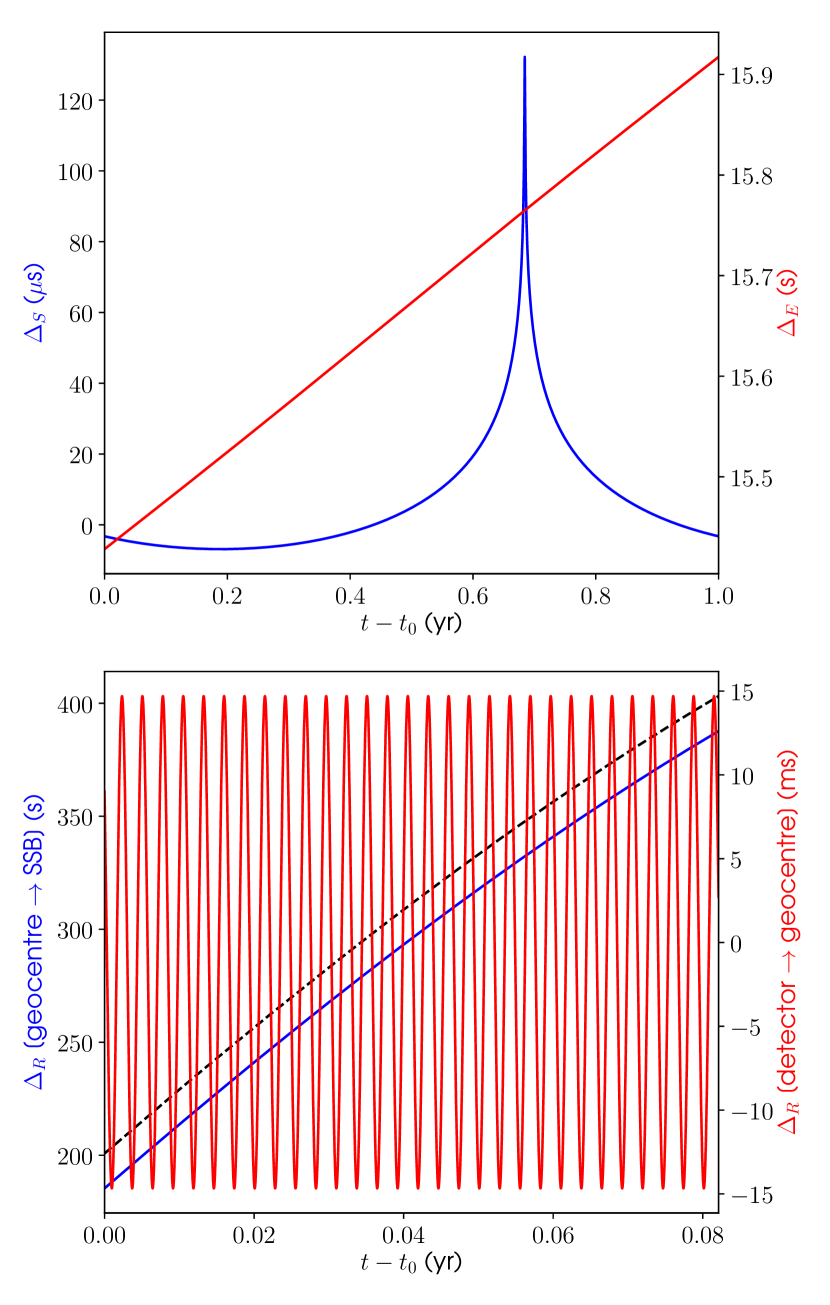
Figure 1: The top panel shows the Shapiro delay (left axis, blue colour) and Einstein delay (right axis, red colour) over one year for a particular sky position ($\alpha=0^{\rm h}$ and $\delta=0\degr$). The bottom panel shows the Roemer delay from the geocentre to the SSB (left-hand axis, blue colour) and from the LIGO Hanford Observatory to the geocentre (right-hand axis, red colour) over one month. The bottom panel also shows the combination of all delays as the dashed black line.

For gravitational waves, unlike electromagnetic signals, we do not require any interstellar dispersion or atmospheric timing corrections, so these can be ignored.

1.2.1 Binary system barycentring

For sources that are in binary or multiple systems, further time delay corrections are required to give an inertial reference frame with respect to the source (e.g., correcting from the binary system barycentre, BSB, to the source frame). This would add a further $\Delta_{\rm B}$ term to Equation 2, i.e.

$$\Delta\tau=\Delta_{R}+\Delta_{E}-\Delta_{S}-\Delta_{B}.$$ (6)

$\Delta_{\rm B}$ consists of the same kind of corrections as required for the SSB, which are nicely described in Taylor & Weisberg (1989), and also in Section 2.7 of Edwards, Hobbs & Manchester (2006). In this analysis we will only focus on binary systems and not multiple systems, and use the model given by Blandford & Teukolsky (1976). From Equation 5 of Taylor & Weisberg (1989) this model is given as

$$\Delta_{B} =\left\{x\sin{\omega_{0}}\left(\cos{E}-e\right)+\left[x\cos{\omega_{0}}\sqrt{1-e^{2}}+\gamma\right]\sin{E}\right\}$$

$$\times\left\{1-\frac{2\pi x}{P_{b}}\frac{[\cos{\omega_{0}}\cos{E}\sqrt{1-e^{2}}-\sin{\omega_{0}}\sin{E}]}{\left(1-e\cos{E}\right)}\right\},$$ (7)

where $x\equiv a\sin{i}/c$ is the projected semi-major axis, $\omega_{0}$ is the longitude of periastron, $P_{b}$ is the orbital period, $e$ is the eccentricity, $\gamma$ measures the gravitational redshift and time dilation (effectively conveying the Einstein delay), and $E$ is the eccentric anomaly defined by

$$E-e\sin{E}=\frac{2\pi}{P_{b}}\left(t_{b}-T_{0}\right),$$ (8)

where $T_{0}$ is the time of periastron passage, and $t_{b}\equiv t+(\Delta_{R}+\Delta_{E}-\Delta_{S})$ is the barycentric time of arrival. From Equations 1.2.1 and 8 it can be seen that the eccentric anomaly is the only time varying term and this enters the binary time delay through its sine and cosine. The eccentric anomaly for a variety of eccentricities over one orbital period is shown in Fig. 2. The Blandford & Teukolsky (1976) model also allows time derivatives of the orbital period, longitude of periastron and eccentricity due to relativistic effects, but here we will ignore them, or assume they vary very little over the period of one orbit.

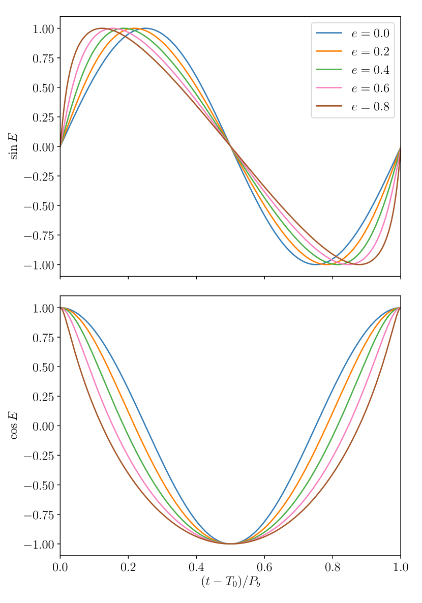
Figure 2: The sine (upper panel) and cosine (lower panel) of the eccentric anomaly (equation 8) for a range of eccentricities

2 Reduced order modelling

In the context of this paper ROM is a method for reducing the computational demand required to produce the model of some process, by using an approximation to that model that is accurate to a given level. In our case the models used are the time delays given by Equations 2 (without the Shapiro delay term) and 1.2.1, computed on a regular grid of time values over one year. This relies on first producing a training set of models spanning some particular required parameter space, empirically finding an orthonormal basis model set from it that can match (or in our case reconstruct) the training set to a given accuracy, and creating an empirical interpolant from it. In our case the empirical interpolant is just a set of times (the number of which is given by the number required orthonormal bases) in the model time series that are found to be optimal for reconstructing the model through linear operations (see Equation 2). The reduced basis and interpolant can be used to reconstruct the model (sometimes called a surrogate model) anywhere within the bounds of the training parameter space. When the number of orthonormal bases is significantly less than the number of points sampling the model, using the interpolant provides a speed-up in calculations, particularly when the model itself is a large computational burden. Here we use ROM as a catch-all term for the entire process of creating a reduced bases set and an empirical interpolant. The first application of this method, and the related reduced order quadrature, to models (and likelihoods) used in gravitational wave data analysis was in Field et al. (2011), and the algorithms are described in detail in Field et al. (2014). Applying the method to computationally demanding compact binary coalescence waveform generation, involving phenomenological spinning signals in particular, has been pioneered by Pürrer (2014) and Smith et al. (2016).

The method used to generate the orthonormal bases from the training set uses a greedy algorithm (it eats the biggest thing first) based on the Gram–Schmidt process, in particular the Iterative Modified Gram–Schmidt (IMGS) algorithm (Hoffmann, 1989). This is implemented in the open source greedycpp code (Antil, Chen & Field, in preparation), which we have modified for our purposes. The basic idea (IMGS has some minor complications) for producing the basis relies on the following steps: pick a model vector from a normalized copy of the training set, and use this as the first basis vector; calculate the projection coefficients of the current basis (just the first basis vector on the first pass) on to all other vectors in the training set (by taking their dot products) and mutliply the basis by these coefficients; get the residual between these projections and the training set, and calculate the projection error (the dot product of each residual vector with itself) for each residual; find the residual with the maximum projection error, normalize it, and take this as a new basis vector; expand the basis set by adding this new basis to it; this process is repeated using the expanded basis until the maximum projection error is below some pre-defined stopping criterion, or tolerance, at which point no more bases are added. The general method is shown as pseudo-code in appendix A of Field et al. (2014), in which the stopping criterion for adding new orthonormal bases to the reduced set is based on the maximum residual projected overlap between the current reduced basis set and the training set. As the reduced basis in the case of Field et al. (2014) is being used to then implement reduced order quadrature, in which dot products of models and data are the desired output, this stopping criterion is sensible. However, for our analysis we are interested in the actual residuals between interpolated models and the training set (the errors in the time delay), and not residuals on projections. Therefore, our modification changes the addition of new orthonormal bases and the stopping criterion to work with absolute residuals. Suppose our model, $h(t;\bm{\mathit{\lambda}})$, is defined by some vector of parameters $\bm{\mathit{\lambda}}$, and we have a training set of $M$ parameter values $\mathcal{T}=\{\bm{\mathit{\lambda}}\}_{i=1}^{M}$ at which the model is evaluated, $\mathcal{B}=\{h(t;\bm{\mathit{\lambda}}_{i})\}_{i=1}^{M}$. Our modification of the algorithm shown in Field et al. (2014) is given in Algorithm 1, which relies on the empirical interpolation method given in appendix B of Field et al. (2014). It should be noted that while the algorithm in Field et al. starts with a normalized set of training models, our method does not as it requires the absolute residuals.

Algorithm 1 A greedy algorithm for creating a reduced basis, adapted from Field et al. (2014, Appendix A).

1:  $i=0$ and $\sigma_{0}=\infty$

2:  choose (arbitrary) seed $\bm{\mathit{\lambda}}\in\mathcal{T}$: e.g., $\bm{\mathit{\Lambda}}_{1}$, $\textbf{{e}}_{1}=h(t;\bm{\mathit{\Lambda}}_{1})$

3:  set initial reduced basis, $\textbf{{R}}=\{\textbf{{e}}_{1}/|\textbf{{e}}_{1}|\}$

4:  while $\sigma_{i}>\varepsilon$ do

5:     $i=i+1$

6:     build interpolant $\mathcal{I}_{i}$ from R

7:     $j=0$

8:     for $j<M$ do

9:        $\textbf{{h}}_{j}=\mathcal{B}_{j}$

10:        create approximant $\bar{\textbf{{h}}}_{j}$ to $\textbf{{h}}_{j}$ using $\mathcal{I}_{i}$

11:        get residual error $r_{j}={\rm max}|\textbf{{h}}_{j}-\bar{\textbf{{h}}}_{j}|$

12:        $j=j+1$

13:     end for

14:     get index with max. residual error, $k={\rm argmax}|r|$

15:     $\sigma_{i}=r_{k}$

16:     $\bm{\mathit{\Lambda}}_{i+1}=\mathcal{T}_{k}$

17:     $h=\mathcal{B}_{k}/|\mathcal{B}_{k}|$ (normalise model)

18:     generate $e_{i+1}$ from $h$ and RB (Gram-Schmidt)

19:     $e_{i+1}=e_{i+1}/|e_{i+1}|$ (normalise new basis)

20:     $\textbf{{R}}=\textbf{{R}}\cup e_{i+1}$ (add to reduced basis)

21:  end while

The output of Algorithm 1 is a reduced basis and the set of greedy points, $\{\bm{\mathit{\Lambda}}_{i}\}_{i=1}^{m}$, where $m$ is the number of bases from which the reduced basis was constructed. If the stopping criterion is not reached until all training points are used, or $m\geq N$, where $N$ is the length of each training model, then it suggests that the training set is largely orthogonal already. If, for example, the training models have been evaluated at a set of $N$ time samples $t_{i}$, then following appendix B of Field et al. (2014) the reduced basis products can then be used to empirically find the $m$ values of $t$, t, that can generate an optimal $m\times m$ interpolation matrix from the reduced basis $\textbf{{S}}=\{h(\textbf{{t}},\bm{\mathit{\Lambda}}_{i})\}_{i=1}^{m}$.

An approximant of the full model at a new point $\bm{\mathit{\lambda}}$ can then be calculated using simple linear algebra, as it is just a weighted sum of the reduced bases. If the model is just evaluated at the $m$ points t, $\textbf{{h}}^{\prime}=h(\textbf{{t}};\bm{\mathit{\lambda}})$, then we can calculate the required weighting coefficients, C, for combining the bases via

$$\textbf{{h}}^{\prime} =\textbf{{C}}\textbf{{S}}$$

C $$=\textbf{{h}}^{\prime}\textbf{{S}}^{-1}.$$ (9)

To reconstruct the full approximated model just requires summing the full reduced basis with appropriate weightings

$$h(t;\bm{\mathit{\lambda}}) =\textbf{{C}}\textbf{{R}}$$

$$=\textbf{{h}}^{\prime}(\textbf{{S}}^{-1}\textbf{{R}}).$$ (10)

The inversion of S just needs to be performed once and stored, meaning the required operations are trivial. Later on we will refer to $\textbf{{V}}=\textbf{{S}}^{-1}\textbf{{R}}$, which again is an operation that just needs to be performed once.

2.1 Reduced order modelling for the SSB

For this work we want to compute the value of $\Delta\tau$ in Equation 2 at a set of discrete times. For a given gravitational wave detector, and a fixed time span, the computation of $\Delta\tau$ only depends on the source’s sky location. In this work we will assume that sources are far enough away that parallax can be ignored, although this could be incorporated in the future. We therefore can create a basis training set using parameters distributed randomly over the sky sphere, which is achieved by drawing points uniformly in right ascension and uniformly in the sine of declination.

Here we will take our baseline as requiring the barycentring time delay to be calculated over one year. To create our training set we draw 5 000 training points in right ascension and declination as described above, and for each pair we calculate $\Delta\tau$ over one year or 365.25 d (arbitrarily starting at 2017 January 1, 00:00:00 UTC, or a GPS time of 1 167 264 018) in 60-s steps. The choices of number of training points and time-step size have been partly guided by computational memory constraints for storing the training set. The time delays are calculated using the JPL DE405 Solar system ephemeris positions, velocities, and accelerations for the Sun and Earth/Moon system (Standish, 1998), and the TCB time coordinate system. Here we have assumed signals arriving at the LIGO Hanford Observatory (H1), but we expect any Earth-bound gravitational wave detector (or indeed any position on the Earth’s surface) to produce very similar results. For our $\Delta\tau$ generation we actually do not include the Shapiro delay term. The Shapiro delay term consists of cusps (see Fig. 1), with the cusp being at different points in the time series for different sky positions (relating to when the Sun is between the Earth and the source). Including Shapiro delay therefore makes it very difficult to produce orthogonal bases across the whole sky. However, the $\textbf{{r}}_{\rm se}$ term in Equation 4 is sky position independent and therefore only needs calculating once over the range of time steps, meaning that the computational burden for determining the Shapiro delay is already low.

We pass the 5 000 sample training set to the modified greedycpp code, which applies Algorithm 1 with the stopping criterion on adding more bases being a maximum time residual of 0.1 s. This stopping criterion looks surprisingly large; however, it was found to lead to a basis that actually produces far smaller time residuals (see section 3) well within the required accuracy of pulsar phase templates for gravitational wave searches.^, We find that only four orthonormal bases are required to reconstruct the training set. These bases are shown in Fig. 3. It can be seen that there are three bases that show dominant yearly periodicities, and one that captures yearly, monthly and daily periodicities. As described in Smith et al. (2016) we have implemented several validation and enrichment steps to confirm that the four bases do not leave gaps in the sky. For each validation we generate 2 000 new randomly distributed training points to give a validation set; the reduced basis is used to create an interpolant to recover each model of the validation set, and any that fail the tolerance test get added to enrich the original training set. The reduced basis can then be rebuilt from the enriched training set. We find that the four originally recovered bases contain no gaps and no enrichment is required. In total 36 000 additional sky locations were tested and all could be reconstructed within the required tolerance (see Fig. 6 and discussions in Section 3.1).

Figure 3: The four orthonormal bases built from the training set covering the sky.

2.2 Reduced order modelling for the BSB

There is also potential to use ROM for the binary system barycentring time delay calculation. As discussed in section 1.2.1 the computational load for this delay is from the calculation of the eccentric anomaly, given by Equation 8. For the binary orbital delay, given in equation 1.2.1, the eccentric anomaly appears through its sine and cosine. So, we construct two ROMs, one for the sine term and one for the cosine term. For a fixed orbital period the eccentric anomaly depends on two variables, the eccentricity, $e$, and the time of periastron passage, $T_{0}$. In producing a ROM we only need to calculate the eccentric anomaly over one orbital period, as the same basis can subsequently be used repeatedly for many orbits. We also only need to produce the ROM for one orbital period at a fixed set of time stamps. For different orbital periods, $P_{b}$, the time stamps used to generate the ROM can be scaled by $P_{b}^{\rm ROM}/P_{b}$ (where $P_{b}^{\rm ROM}$ is the fixed period used in calculating the ROM), and the eccentric anomaly components reconstructed from the basis can be interpolated on to the actual data time stamps.

As an example, here we constructed a ROM using a 5 000 point training set covering a range of eccentricities from zero to 0.25. The eccentricities are drawn uniformly over this range. We, somewhat arbitrarily, chose to fix the orbital period to 3 600 s, and therefore have training points in $T_{0}$ sampled uniformly between 0 and 3 600 s. Each model ($\sin{E}$ and $\cos{E}$) in the training set is calculated at time stamps that span one orbital period and spaced at one second intervals (i.e. there are 3 601 time points). To produce the ROMs we set a tolerance for the maximum timing error of 10 ns at which to stop adding more bases. The first five bases for $\sin{E}$ and $\cos{E}$, given as a function of orbital period, are shown in Fig. 4. Unlike for the Solar system barycentring ROM we are treating this as a toy problem and we have therefore not gone to the lengths of performing any validation or enrichment steps in the basis generation, although we do not expect there to be significant gaps in the basis.

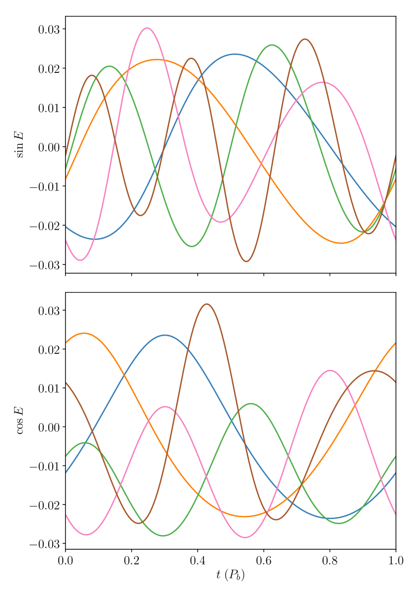
Figure 4: The first five basis vectors of the sine and cosine of the eccentric anomaly for a maximum eccentricity of 0.25.

We find that for an eccentricity of 0.25 the residual tolerance requires 34 bases for both the $\sin{E}$ and $\cos{E}$ terms, which can be compared to the 3 601 time points used. Fig. 5 also shows how the number of required bases varies with eccentricity. It can be seen that for fully circular orbits only three bases are required for both the sine and cosine components, whilst for highly eccentric orbits ($e=0.9$) over 500 bases are required. It is also interesting to note that for ellipticities $\lesssim 0.5$ the cosine term always requires bases greater than, or equal to, the number of bases for the sine term, while at larger values the sine term generally requires more bases.

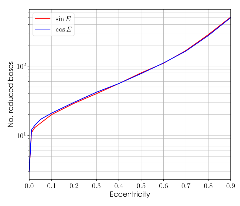
Figure 5: The number of reduced bases required for reconstructing the sine and cosine of the eccentric anomaly as a function of eccentricity.

3 Timing and accuracy

The reason for producing the reduced bases and empirical interpolants is to provide a computational speed-up in calculating Equations 2 and 1.2.1 without any impact on the required precision. Here we provide timings of these calculations when evaluating the functions explicitly at all required time-steps and compare them to the timings when using the reduced basis and empirical interpolants. We also assess the accuracy of the reconstructed time delays by looking at the residual differences between the full evaluations and interpolated versions.

We should note that the production of the ROM does require some overhead: of the order of 10 min for the Solar system barycentring time delays, and tens of seconds for the eccentric anomaly. However, these overheads are one-off requirements compared to the huge number of times the full functions might be needed.

3.1 Solar system barycentring

Above we found that the model given by Equation 2 (with the Shapiro delay term removed) can be approximated for any position on the sky using just four basis vectors. During the validation of the reduced basis a total of 36 000 sky points were tested, for which the basis and empirical interpolant generated from it were used to reproduce the time delay over the full grid of time-steps at which the basis was produced. Residual time delays calculated by subtracting these reconstructed delays from those explicitly calculated for the given sky position have a maximum absolute value of $7.4\!\times\!10^{-4}$ ns. A histogram of the maximum absolute residual for each of the 36 000 test points is shown in Fig. 6, along with an example of the residual time series (which in this case also includes the Shapiro delay as calculated using equations 4 and 1.2, with $\textbf{{r}}_{\rm se}$ and $\left|\textbf{{r}}_{\rm se}\right|$ pre-computed). The accuracy achieved is far better than any requirements for residual phase uncertainties in a pulsar model.

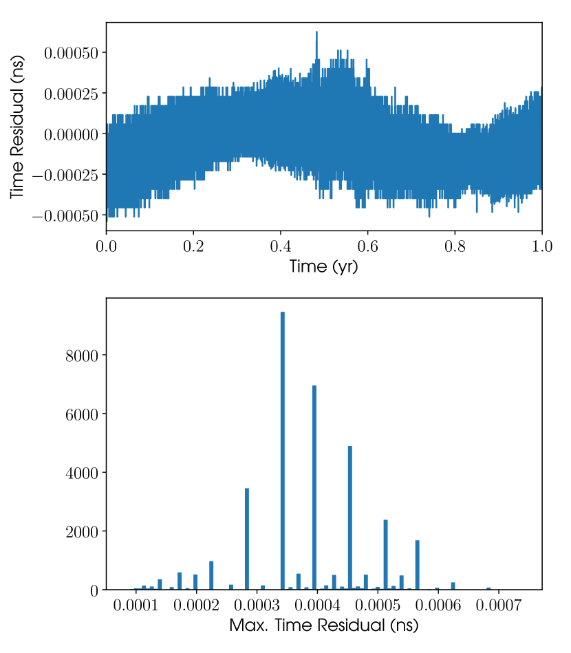
Figure 6: The upper panel shows an example of the timing residuals between the explicit evaluation of $\Delta\tau$ over one year and the reconstruction using the ROM and empirical interpolant. The lower panel shows a histogram of the absolute maximum timing residual for reconstructions at 36 000 sky locations.

We also need to show that this basis can speed-up calculations when compared to explicitly calculating the time delay at the same number of time-steps as used in the basis. When using the ROM to reconstruct the time delay for a given sky position there are several things that need to be calculated: there is a one-off evaluation of $\textbf{{V}}=\textbf{{S}}^{-1}\textbf{{R}}$ from Equation 2; the time delay needs to be explicitly calculated at the four empirical interpolant nodes, $\textbf{{h}}^{\prime}$; the dot product $\textbf{{h}}^{\prime}\textbf{{V}}$; the Shapiro delay, using pre-computed sky-position independent vectors for $\textbf{{r}}_{\rm se}$ and $\left|\textbf{{r}}_{\rm se}\right|$; and, finally, the reconstructed time delay and Shapiro delay need to be combined. The timings for these various steps, and the ordering of the steps that must be re-computed for different parameters, are given in Table 1. To explicitly calculate the SSB time delay at the 525 960 time points over the year takes $\sim 7.6\!\times\!10^{5}\,\mu$s, whilst using the ROM takes $A_{1}+B_{1}+C_{1}+D_{1}\approx 2.7\!\times\!10^{4}\,\mu$s (where we ignore the one-off calculations), showing a speed-up factor of $\lesssim 30$. The vast majority of the computation time comes from the Shapiro delay step.

Table 1: Computational evaluation times for aspects of the Solar system barycentring time delay

Order	Function	Time ($\mu s$)
	$\Delta\tau$ (525 690 evaluations)a	$\sim 7.6\!\times\!10^{5}$
	$\Delta\tau$ (1 evaluation)a	$\sim 1.4$
	$\textbf{{V}}=\left(\textbf{{S}}^{-1}\textbf{{R}}\right)$b	$\sim 1.1\!\times\!10^{4}$
$A_{1}$	$\textbf{{h}}^{\prime}=\Delta\tau^{\rm no\leavevmode\nobreak\ Shap.}$ (4 evaluations)	$\sim 5.7$
$B_{1}$	$(\Delta\tau)_{\rm int}^{\rm no\leavevmode\nobreak\ Shap.}=\textbf{{h}}^{\prime}\textbf{{V}}$	$\sim 1.6\!\times\!10^{3}$
$C_{1}$	Shapiro delayc	$\sim 2.4\!\times\!10^{4}$
$D_{1}$	$(\Delta\tau)_{\rm int}^{\rm no\leavevmode\nobreak\ Shap.}-$ Shapiro delay	$\sim 820$
a Equation 2
b see Equation 2
c Shapiro delay calculated using pre-computed $\textbf{{r}}_{\rm se}$ & $\left|\textbf{{r}}_{\rm se}\right|$

3.1.1 Further interpolation

The training set, and therefore the reduced basis vectors, for the SSB delay is calculated on a time grid at 60-s intervals. However, values of the delay at time values between these grid points may well be required. Such values can be calculated by creating interpolation functions for the reduced bases. When reconstructing a time delay vector we work with the matrix $\textbf{{V}}=\textbf{{S}}^{-1}\textbf{{R}}$ from Equation 2, which in this case is $4\times 525\,690$ in size. For each of the four rows we can create a cubic B-spline interpolation function [using the splrep and splev functions from scipy’s (Jones et al., 2001) interpolate module for generating and evaluating the interpolation function, respectively]; we can also do this for the vectors required for the Shapiro delay calculation: the three components of $\textbf{{r}}_{\rm se}$ and $\left|\textbf{{r}}_{\rm se}\right|$. Creation of each of these interpolation functions takes $\sim 10^{5}\,\mu$s each, although these are one-off evaluations.

We have tested the accuracy of the interpolations by creating a new set of time-steps half-way between those used for the basis generation, i.e. at 60 second intervals, but all maximally offset by 30 s. Each of the eight spline interpolation functions (the four rows of V and the four vectors for the Shapiro delay calculation) was evaluated at these new time stamps, to give new matrices $\textbf{{V}}^{\prime}$, $\left|\textbf{{r}}_{\rm se}\right|^{\prime}$, and $\textbf{{r}}_{\rm se}^{\prime}$. The evaluations each took $\sim 3.0\!\times\!10^{4}\,\mu$s, but again these are sky-position independent and therefore one-off calculations, so do not affect overall speed-up of the time delay calculation. From these, the time delays were reconstructed as above for 100 random sky locations. Examples of the residuals between them and explicit evaluation of the time delays at the new time points, along with a histogram of the residuals, are shown in Fig. 7. In the example residuals, it would appear at first glance that the errors are of the order of hundreds of nanoseconds, which are acceptable, but not as good as might be hoped given the extraordinary agreement when not interpolating between time-steps shown in Fig. 6. However, the zoom-in of the time series also shown in Fig. 7, and the histograms of residuals, shows that the largest errors occur as spikes every four hours, whilst between these spikes the residuals are far smaller; we find that $\lesssim 8\%$ of times produce residuals larger than the value of $7.4\!\times\!10^{-4}$ ns seen above as the maximum value in Fig. 6, $\lesssim 2.6\%$ have residuals larger than 1 ns, and $\lesssim 1.2\%$ have residuals larger than 10 ns. We find that these spikes are due to the 4-h sample rate of Earth ephemeris (position, velocity, and accelations) values (derived from the JPL ephemerides Standish, 1998) used in the ephemeris files within LALSuite (the Sun ephemeris has a 40-h sample rate that falls on the time bins for the Earth data); within the LALSuite barycentring routines the extrapolation of the Earth’s position and velocity between these samples leads to minor discontinuities at the joins (half way between each sample), and the cubic spline produces an impulse response at these joins.

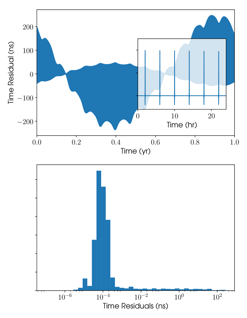
Figure 7: The upper panel shows an example of the timing residuals between the explicit evaluation of $\Delta\tau$ over one year and the reconstruction using the ROM interoplated using a cubic B-spline at time stamps half-way between those used to create the ROM basis. The inset in the upper panel shows a zoom of the residuals for one day. The lower panel shows a histogram of the absolute timing residual for reconstructions at 100 sky locations.

The full years worth of time delay calculations will not be required for all analyses, many of which would use shorter subsets of data. Therefore, using the full length of the reduced basis when calculating the the time delays over the required period would be more computationally demanding than necessary. However, the full reduced basis is not required and the a submatrix of the reduced basis matrix R in Equation 2 can just be used that spans the required times values.

3.2 Binary system barycentring

For the binary system time delay model described in Sections 1.2.1 and 2.2 we found that for eccentricities of $\leq 0.25$ 34 reduced bases were required for both the $\sin{E}$ and $\cos{E}$ terms. The evaluation times for various functions are provided in Table 2, where the order of operations required for the ROM interpolant (following its generation) are given. The time to calculate $\Delta_{B}$ using the ROM interpolant is therefore given by $\sim 2A_{2}+2B_{2}+C_{2}\approx 130$ $\mu$s. Compared to the reference time of 1 600 $\mu$s given in the first line of Table 2 this shows that using the interpolant can speed up the computation by $\sim 12$ times.

Table 2: Computational evaluation times for aspects of the binary system time delay

Order	Function	Time ($\mu s$)
	$\Delta_{B}$ (3 601 evaluations)a	$\sim 1\,600$
	$\Delta_{B}$ (1 evaluation)a	$\sim 0.5$
	$\textbf{{V}}_{\sin{E}/\cos{E}}=\left(\textbf{{S}}^{-1}\textbf{{R}}\right)$b	$\lesssim 2\,200$
$A_{2}$	$\textbf{{h}}^{\prime}=\sin{E},\cos{E}$ (34 evaluation)	$\sim 20$
$B_{2}$	$(\sin{E}/\cos{E})_{\rm int}=\textbf{{h}}^{\prime}\textbf{{V}}$	$\sim 27$
$C_{2}$	$\Delta_{B}$ (using $(\sin{E}/\cos{E})_{\rm int}$)c	$\sim 38$
a Equation 1.2.1
b see Equation 2
c using Equation 1.2.1, but with interpolated $\sin{E}$ and
$\cos{E}$ vectors.

The accuracy (maximum residual time) with which the ROM reconstructs both the sine/cosine of the eccentric anomaly and the binary time delay $\Delta_{B}$ over one orbital period is shown in Fig. 8 for 10 000 randomly generated set of binary system parameters. The red solid and dashed histograms show that the reconstructed $\sin{E}$ and $\cos{E}$ values are always within the tolerance of 10 ns used when producing the reduced basis. The histograms shown as the shaded area and the solid blue line show cases where the binary period for all systems has been held fixed at the 1-h value used in the training set generation. For the histogram shown as the solid blue line, the ROM reconstructed binary time delays have been subsequently interpolated (using a cubic B-spline interpolator) on to time-steps half-way between those used for the ROM generation, and compared to the evaluation of the full time delay at those new time-steps. The histogram represented by the black solid line shows the case when the period has been drawn uniformly between 10 mins and 10 h, for which the interpolant time-steps have been rescaled by $(P_{b}/1\,{\rm hour})$, and again a cubic B-spline interpolator used to re-sample to the required time-steps. The accuracy of $\Delta_{B}$ is not able to match that for $\sin{E}$ and $\cos{E}$ alone, as the errors on these propagate into $\Delta_{B}$ with a potential increased by a factor on the order of the value of $a\sin{i}/c$, which leads to larger errors. However, we find that for all cases (given that our range of $a\sin{i}/c$ values are restricted to $<100$ s) less than 2% of our systems lead to errors on $\Delta_{B}$ of greater than 100 ns, with maximum errors of $\sim 500$ ns.

As mentioned above, it may be required to evaluate the function $\Delta_{B}$ at time-steps that are not the same as those used in the training set generation, or for different binary periods. This means that further interpolation is required, which could reduce the speed-up that the ROM interpolation gives. If, as for the SSB case, we use a cubic B-spline, then the interpolation function generation using 3 601 time points takes $\sim 500\,\mu{\rm s}$ and evaluation, again at 3 601 new time points, takes $\sim 270\,\mu$s. So, if interpolation to new times is required the total time is (again taking values from Table 2) $\sim 130+500+270\approx 900\,\mu{\rm s}$, which only shows a speed-up of just under two times. Unlike for the SSB case, if the binary period is a parameter that is changing, then we cannot produce one-off interpolation functions for each component of the $\textbf{{V}}=\textbf{{S}}^{-1}\textbf{{R}}$ matrix, as the interpolation time-steps have to be scaled by the period.

Performing a simpler linear interpolation only takes $\sim 100\,\mu{\rm s}$, but produces a mean error in the time delay of $\sim 10\,000$ ns with a maximum around 1 ms.

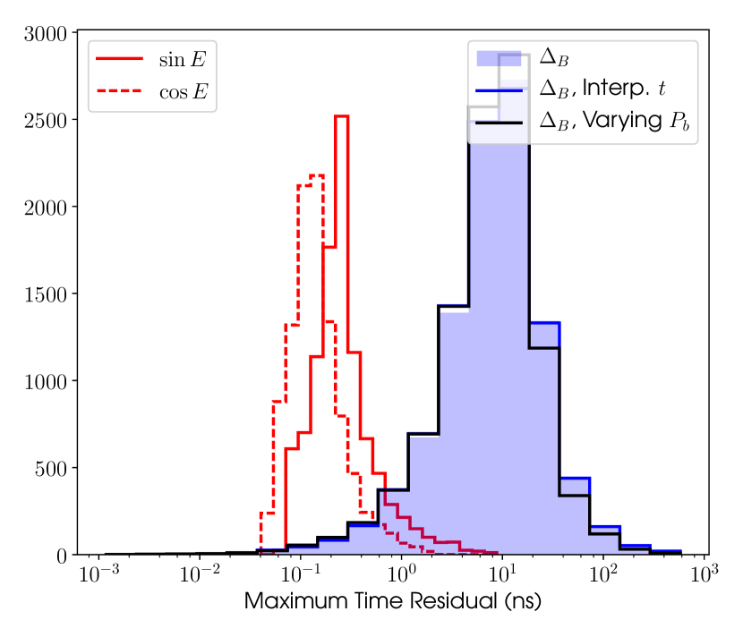
Figure 8: Histograms of maximum residuals between the functions $\sin{E}$, $\cos{E}$ and $\Delta_{B}$ as explicitly evaluated and reconstructed using the ROM.

4 Application

It is useful to estimate how the speed-up demonstrated above could be applied in real searches for continuous gravitational wave signals. The time $\tau$ taken to perform coherent matched-filtering of a single continuous wave signal template can be modelled as (Prix, 2017):

$$\tau=\tau_{\text{core}}+b\tau_{\text{bary}}$$ (11)

when $\tau_{\text{core}}$ is the time taken to perform the core filtering operations, $\tau_{\text{bary}}$ is the time taken to perform solar system and/or binary system barycentering. It is usual to buffer the barycentered time series if the sky position and/or binary system parameters have not changed from the previously-analysed signal template; conversely when the sky position and/or binary system parameters do change, the barycentered time series must be recomputed for the new parameters. The fraction of signal templates where barycentering must be re-performed is denoted $b$. The value of $b$ largely depends on the design of the search algorithm and the parameter-space being searched. For search algorithms that do not use a search grid but rather compute templates at randomly chosen parameters (e.g. Shaltev & Prix, 2013; Shaltev et al., 2014; Ashton, 2017; Ashton & Prix, 2018) we have $b=1$.

The speed-up of such a search $x_{\text{search}}$ due of the use of a ROM may be quantified using Eqn. (11) as

$$\begin{split}x_{\text{search}}&=\frac{\tau_{\text{core}}+\tau_{\text{bary}}}{\tau_{\text{core}}+\tau_{\text{bary}}/x_{\text{ROM}}}\\ &=\frac{1+x^{\text{bary}}_{\text{core}}}{1+x^{\text{bary}}_{\text{core}}/x_{\text{ROM}}}\end{split}$$ (12)

where $x_{\text{ROM}}$ is the speed-up from the use of a ROM, and $x^{\text{bary}}_{\text{core}}$ is the fraction of time spent computing the (non-ROM) barycentering, relative to performing the core filtering. Representative values of $x^{\text{bary}}_{\text{core}}$ are $\sim 17$ for sky demodulation and $\sim 23$ for binary demodulation. Given a speed-up of $x_{\text{ROM}}\sim 30$ or $12$ from the use of a ROM for sky or binary demodulation, potential search speed-ups are $x_{\text{search}}\sim 11$ or $8$ respectively.

5 Conclusions

In this paper we have aimed to show that ROM can be used as a way to approximate the time delays required to transform a signal received at an observatory on Earth to the inertial frame of the Solar system (or binary system) barycentre. For the Solar system this transformation is sky-position dependent, and if requiring coherent integration of signals over long periods its recalculation can become a computational burden. In particular, this could be an issue for some large sky area searches for continuous gravitational wave sources, or the long-coherent time follow-up of candidates from such searches (Shaltev & Prix, 2013; Shaltev et al., 2014; Ashton, 2017; Ashton & Prix, 2018). We have shown that the Solar system barycentring time delay function can be very well approximated using just four basis vectors, when excluding the Shapiro delay. Using this reduced basis can significantly speed up the calculation of the time delays by up to a factor of 30, even when adding on the computation of the Shapiro delay term. In general the reconstructed time delays are accurate to sub-nanosecond precision when compared to the full calculation. If time delays needs to be calculated at time stamps not used for the reduced basis production, then additional interpolation of the basis vectors can be used. In this case it, is found that for a few percent of the samples the reproductions are accurate only to within $\sim 100$ ns. This larger residual has been found to be a feature of the sample rate of the Solar system ephemeris files within LALSuite (LIGO Scientific Collaboration, 2017).

In cases where SSB time delay calculations are a bottleneck in analyses, for example, if having to search over a large number of sky positions in long data sets, this will reduce the computational burden and may allow larger parameter spaces to be searched. The barycentre time delay model used in this work does not include all the components used in, for example, the pulsar timing software tempo2 (Edwards, Hobbs & Manchester, 2006). However, in the future it may well be straightforward to incorporate the tempo2 timing model into greedycpp (Antil et al., in preparation). In the future the timing routines in LALSuite (LIGO Scientific Collaboration, 2017) could be adapted to incorporate the ROMs, as produced using the tempo2 model, and thus ensure consistency between the two code bases.

In addition to SSB time delays, we have also looked at the calculations required for time delay in binary systems. The main computational burden in such calculations is the eccentric anomaly. We have shown that for eccentricities of $<0.25$ a reduced basis of 34 vectors is required to reproduce the sine and cosine of the eccentric anomaly to a precision of less than 10 ns. In the simplest cases, when not varying the binary orbital period, factors of $\sim 10$ speed-up in the time delay calculation are found.

Outside of the initial application of this method for continuous gravitational wave sources with Earth-bound detectors, there are other areas where it could be used. For third-generation gravitational wave detectors (e.g., the Einstein Telescope, Abernathy et al., 2011, or Cosmic Explorer, Abbott et al., 2017b), the signals from compact binary coalescences may be within the sensitivity bands for days, so coherent integration will have to account for Earth rotational and orbital motion using the delays discussed here. For future space-based gravitational wave detectors (e.g., LISA Amaro-Seoane et al., 2013; Danzmann et al., 2017) the majority of the expected signals will be quasi-continuous and long-lived within the detector’s sensitive band. The orbital motion of the spacecraft will need to be accounted for when searching for signals and the ROM method applied here could be very useful. This approach may also be useful for standard pulsar timing applications, especially in cases where the number of time-of-arrival observations become large, and sky positions need to be incorporated into parameter fits. Methods that have to sample over parameter spaces such as temponest (Lentati et al., 2014) or bayesfit (Vigeland & Vallisneri, 2014) may particularly benefit from faster model evaluations.

In a future paper we will study how ROM methods, and the related reduced order quadrature, can be used to speed-up likelihood evaluations in searches for gravitational waves from pulsars. The method has already been applied in the search of LIGO data for signals from known pulsars in Abbott et al. (2017c).

References

- Abbott et al. (2004) Abbott B., Abbott R., Adhikari R., et al., 2004, Phys. Rev. D, 69, 082004
- Abbott et al. (2008) Abbott B., Abbott R., Adhikari R., et al., 2008, Phys. Rev. D, 77, 022001
- Abbott et al. (2009) Abbott B., Abbott R., Adhikari R., et al., 2009, Phys. Rev. D, 79, 022001
- Abbott et al. (2017a) Abbott B. P., Abbott R., Abbott T. D., et al., 2017a, Phys. Rev. D, 96, 062002
- Abbott et al. (2017b) Abbott B. P., Abbott R., Abbott T. D., et al., 2017b, Classical Quantum Gravity, 34, 044001
- Abbott et al. (2017c) Abbott B. P., Abbott R., Abbott T. D., et al., 2017c, ApJ, 839, 12
- Abernathy et al. (2011) Abernathy M., Acernese F., Ajith P., et al., 2011, Einstein gravitational wave telescope conceptual design study. Tech. Rep. ET-0106C-10, European Gravitatioanl Observatory, http://www.et-gw.eu/
- Amaro-Seoane et al. (2013) Amaro-Seoane P. et al., 2013, GW Notes, 6, 4
- Ashton (2017) Ashton G., 2017, PyFstat-v1.1.0. 10.5281/zenodo.1069408
- Ashton & Prix (2018) Ashton G., Prix R., 2018, arXiv:1802.05450
- Astone et al. (2002) Astone P., Borkowski K. M., Jaranowski P., Królak A., 2002, Phys. Rev. D, 65, 042003
- Behnel et al. (2011) Behnel S., Bradshaw R., Citro C., Dalcin L., Seljebotn D., Smith K., 2011, Computing in Science & Engineering, 13, 31 , http://cython.org
- Blandford & Teukolsky (1976) Blandford R., Teukolsky S. A., 1976, ApJ, 205, 580
- Brady & Creighton (2000) Brady P. R., Creighton T., 2000, Phys. Rev. D, 61, 082001
- Brady et al. (1998) Brady P. R., Creighton T., Cutler C., Schutz B. F., 1998, Phys. Rev. D, 57, 2101
- Danzmann et al. (2017) Danzmann K., et al., 2017, LISA: Laser Interferometer Space Antenna. https://www.elisascience.org/files/publications/LISA_L3_20170120.pdf
- Droettboom et al. (2017) Droettboom M., Caswell T. A., Hunter J., et al., 2017, matplotlib/matplotlib: v2.0.0. 10.5281/zenodo.248351
- Edwards, Hobbs & Manchester (2006) Edwards R. T., Hobbs G. B., Manchester R. N., 2006, MNRAS, 372, 1549
- Field et al. (2011) Field S. E., Galley C. R., Herrmann F., et al., 2011, Phys. Rev. Lett., 106, 221102
- Field et al. (2014) Field S. E., Galley C. R., Hesthaven J. S., et al., 2014, Phys. Rev. X, 4, 031006
- Hobbs, Edwards & Manchester (2006) Hobbs G. B., Edwards R. T., Manchester R. N., 2006, MNRAS, 369, 655
- Hoffmann (1989) Hoffmann W., 1989, Computing, 41, 335
- Hunter (2007) Hunter J. D., 2007, Computing In Science & Engineering, 9, 90
- Jaranowski, Królak & Schutz (1998) Jaranowski P., Królak A., Schutz B. F., 1998, Physical Review D, 58, 063001
- Jones et al. (2001) Jones E., Oliphant T., Peterson P., et al., 2001, SciPy: Open source scientific tools for Python. http://www.scipy.org/
- Kluyver et al. (2016) Kluyver T. et al., 2016, in Positioning and Power in Academic Publishing: Players, Agents and Agendas: Proceedings of the 20th International Conference on Electronic Publishing, Loizides F., Schmidt B., eds., IOS Press, p. 87, http://jupyter.org/
- Krishnan et al. (2004) Krishnan B., Sintes A. M., Papa M. A., Schutz B. F., Frasca S., Palomba C., 2004, Phys. Rev. D, 70, 082001
- Lentati et al. (2014) Lentati L., Alexander P., Hobson M. P., et al., 2014, MNRAS, 437, 3004, https://github.com/LindleyLentati/TempoNest
- LIGO Scientific Collaboration (2017) LIGO Scientific Collaboration, 2017, LALSuite. https://wiki.ligo.org/DASWG/LALSuite
- Lyne & Graham-Smith (1998) Lyne A. G., Graham-Smith F., 1998, Pulsar Astronomy, 2nd edn., 31. Cambridge University Press
- Manchester et al. (2005) Manchester R. N., Hobbs G. B., Teoh A., Hobbs M., 2005, AJ, 129, 1993, http://www.atnf.csiro.au/people/pulsar/psrcat/
- Pérez & Granger (2007) Pérez F., Granger B. E., 2007, Computing in Science and Engineering, 9, 21, http://ipython.org
- Pletsch (2010) Pletsch H. J., 2010, Phys. Rev. D, 82, 042002
- Prix (2017) Prix R., 2017, Characterizing timing and memory-requirements of the f-statistic implementations in lalsuite. Tech. Rep. LIGO-T1600531, LIGO
- Pürrer (2014) Pürrer M., 2014, Classical and Quantum Gravity, 31, 195010
- Sathyaprakash & Schutz (2009) Sathyaprakash B. S., Schutz B. F., 2009, Living Rev. Relativ., 12, 2
- Schutz & Papa (1999) Schutz B. F., Papa M. A., 1999, arXiv:gr-qc/9905018
- Shaltev et al. (2014) Shaltev M., Leaci P., Papa M. A., Prix R., 2014, Phys. Rev. D, 89, 124030
- Shaltev & Prix (2013) Shaltev M., Prix R., 2013, Phys. Rev. D, 87, 084057
- Smith et al. (2016) Smith R., Field S. E., Blackburn K., et al., 2016, Phys. Rev. D, 94, 044031
- Standish (1998) Standish E. M., 1998, JPL Planetary and Lunar Ephemerides, DE405/LE405. NASA Jet Propulsion Laboratory, Pasadena, IOM 312.F-98-048
- Taylor & Weisberg (1989) Taylor J. H., Weisberg J. M., 1989, ApJ, 345, 434
- Thorne (1987) Thorne K. S., 1987, in Three hundred years of gravitation, Hawking S. W., Israel W., eds., Cambridge University Press
- Vigeland & Vallisneri (2014) Vigeland S. J., Vallisneri M., 2014, MNRAS, 440, 1446, https://github.com/vallis/mc3pta/tree/master/bayesfit
- Wette (2014) Wette K., 2014, Phys. Rev. D, 90, 122010
- Wette (2015) Wette K., 2015, Phys. Rev. D, 92, 082003
- Williams & Schutz (2000) Williams P. R., Schutz B. F., 2000, in AIP Conference Series, Meshkov S., ed., Vol. 523, pp. 473–476