Correct energy evolution of stabilized formulations: The relation between VMS, SUPG and GLS via dynamic orthogonal small-scales and isogeometric analysis.
II: The incompressible Navier–Stokes equations

Abstract

This paper presents the construction of a correct-energy stabilized finite element method for the incompressible Navier-Stokes equations. The framework of the methodology and the correct-energy concept have been developed in the convective–diffusive context in the preceding paper [M.F.P. ten Eikelder, I. Akkerman, Correct energy evolution of stabilized formulations: The relation between VMS, SUPG and GLS via dynamic orthogonal small-scales and isogeometric analysis. I: The convective–diffusive context, Comput. Methods Appl. Mech. Engrg. 331 (2018) 259–280]. The current work extends ideas of the preceding paper to build a stabilized method within the variational multiscale (VMS) setting which displays correct-energy behavior. Similar to the convection–diffusion case, a key ingredient is the proper dynamic and orthogonal behavior of the small-scales. This is demanded for correct energy behavior and links the VMS framework to the streamline-upwind Petrov-Galerkin (SUPG) and the Galerkin/least-squares method (GLS).

The presented method is a Galerkin/least-squares formulation with dynamic divergence-free small-scales (GLSDD). It is locally mass-conservative for both the large- and small-scales separately. In addition, it locally conserves linear and angular momentum. The computations require and employ NURBS-based isogeometric analysis for the spatial discretization. The resulting formulation numerically shows improved energy behavior for turbulent flows comparing with the original VMS method.

1 Introduction

The creation of artificial energy in numerical methods is undesirable from both a physical and a numerical stability point of view. Therefore methods precluding this deficiency are often sought after. This work continues the construction of the correct-energy displaying stabilized finite element methods. The first episode [1] exposes the developed methodology in the convective–diffusive context. The current study deals with the incompressible Navier–Stokes equations and is the second piece of work within the framework. The setup of this paper is closely related to that of [1]. In particular, the correct-energy demand is the same, thus it represents that the method (i) does not create artificial energy and (ii) closely resembles the energy evolution of the continuous setting. The precise definition is stated in Section 4. What sets the Navier–Stokes problem apart from convection–diffusion case is the inclusion of the incompressibility constraint. In this work we use a divergence-conforming basis which allows exact pointwise satisfaction of this constraint. This is considered a beneficial property. Therefore it is added as a design criterion. In a two-phase context this property is essential for correct energy behavior [2].

1.1 Contributions of this work

This paper derives a novel VMS formulation which exhibits the correct energy behavior and to this purpose combines several ingredients. The final formulation is summarized in A. The new method is a residual-based approach that employs (i) dynamic behavior of the small-scales, (ii) solenoidal NURBS basis functions and (iii) a Lagrange-multiplier construction to ensure the incompressibility of the small-scale velocities. The formulation is of skew-symmetric type, rather than conservative, which is motivated by both the correct-energy demand and its improved behavior in the single scale setting (i.e. the Galerkin method) [3]. Moreover, the formulation reduces to a Galerkin formulation in case of a vanishing Reynolds number due to a Stokes-projector. The use of dynamic small-scales, firstly proposed in [4], is also driven from an energy point of view. In addition, it leads to global momentum conservation and the numerical results of [5] show improved behavior of the dynamic small-scales with respect to their static counterpart.

1.2 Context

This work falls within the variational multiscale framework [6, 7]. The basic idea of this method is to split solution into the large/resolved-scales and small/unresolved-scales. The small-scales are modeled in terms of (the residual of) the large scales and substituted into the equation for the large-scales. This approach was first applied in a residual-based LES context to incompressible turbulence computations in [8]. The VMS methodology has enjoyed a lot of progress since then. For an overview of the development consult the review paper [9].

Our work is not the first to analyze the energy behavior of the VMS method. A spectral analysis of the VMS method can be found in [10]. That paper proves dissipation of the model terms under restrictive conditions. Additional to the optimality projector, they require $L_{2}$-orthogonality of the large- and small-scales. This condition naturally leads to the use of spectral methods.

Principe et al. [11] provide a precise definition of the numerical dissipation within the variational multiscale context for incompressible flows. Equally important, they numerically show that the concept of dynamic small-scales, which we apply in this work, is able to model turbulence.

Colomés et al. [12] assess the performance of several VMS methods for turbulent flow problems and provide an energy analysis of these methods. They conclude that algebraic subgrid scales (ASGS) and orthogonal subscales (OSS) yield similar results, whereas the latter one is more convenient in terms of numerical performance.

We build onto [10, 11, 12] without requiring $L_{2}$-orthogonality. Therefore we are not restricted to the use of spectral methods, while retaining a strict energy relation.

Other recent related work includes the IGA divergence-conforming VMS method of Opstal et al. in [13]. They also employ an $H_{0}^{1}$-orthogonality between the velocity large- and small-scales on a local level. Our work deviates from [13] in that we motivate the required orthogonalities with the correct energy demand. Furthermore, our work distinguishes itself by enforcing the divergence-free velocity small-scales with a Lagrange-multiplier construction. We believe the Stokes orthogonality between the large- and small-scales is a natural path to take, since it reduces the scheme to the Galerkin method in the vanishing Reynolds number limit.

The discretizations throughout this work are based on the isogeometric analysis (IGA) concept, proposed by Hughes et al. in [14]. This idea integrates the historically distinct fields of computer aided design (CAD) and finite element analysis. Isogeometric analysis rapidly became a valuable tool in computational fluid dynamics, in particular in turbulence computations. It provides several advantages over standard finite element analysis, including an exact description of CAD geometries, increased robustness and superior approximation properties [14, 15, 16]. This work requires in particular inf–sup stable discretizations for which we use [17, 18]. Moreover these spaces allow the pointwise satisfaction of the incompressibility constraint. The smooth NURBS basis functions are convenient for the computation of second derivatives.

1.3 Outline

The organization of this paper in Section 2 and 3 is very comparable with that of the convective–diffusive context [1], and at some points mirrors it. The purpose thereof is (i) to indicate the great similarities of the methodologies and (ii) to clarify the approach. The remainder of this paper presents the actual construction of a stabilized variational formulation for the incompressible Navier–Stokes equations which displays correct-energy behavior. We summarize it as follows. Section 2 states the continuous form of the governing incompressible flow equations, both in the strong formulation and the standard weak formulation. It additionally provides the energy evolution of the continuous equation, in both global and local form. Section 3 discusses the energy evolution of the variational multiscale approach with dynamic small-scales. The path toward correct energy behavior actually starts in Section 4. This Section presents the required orthogonality of the large-scales and small-scales. This converts the residual-based variational multiscale method into the Galerkin/least-squares method with the correct energy behavior. Section 5 presents conservation properties of the method. Section 6 provides a computational test case, namely a three-dimensional Taylor–Green vortical flow. In particular it examines the energy behavior and compares the novel method with the standard VMS method with static small-scales [8]. The calculations employ the generalized-$\alpha$ method with favorable energy behavior which is also discussed in [1]. In Section 7, we wrap up and present avenues for future research.

2 The continuous incompressible Navier–Stokes equations

2.1 Strong formulation

Let $\Omega\in\mathbb{R}^{d}$, $d=2,3$, denote the spatial domain and $\partial\Omega=\Gamma=\Gamma_{g}\cup\Gamma_{h}$ its boundary, see Figure 1.

Figure 1: Spatial domain $\Omega$ with its boundaries $\Gamma=\Gamma_{g}\cup\Gamma_{h}$. This is the same figure as in [1].

The problem consists of solving the incompressible Navier–Stokes equations governing the fluid flow, which read in strong form

$$\partial_{t}\mathbf{u}+\nabla\cdot\left(\mathbf{u}\otimes\mathbf{u}\right)+\nabla p-\nabla\cdot\left(2\nu\nabla^{s}\mathbf{u}\right)=\mathbf{f} \quad\text{in}\quad\Omega\times\mathcal{I},$$ (1a)

$$\nabla\cdot\mathbf{u}=0 \quad\text{in}\quad\Omega\times\mathcal{I},$$ (1b)

$$\mathbf{u}=\mathbf{g} \quad\text{in}\quad\Gamma_{g}\times\mathcal{I},$$ (1c)

$$-u_{n}^{-}\mathbf{u}-p\mathbf{n}+\nu\partial_{n}\mathbf{u}=\mathbf{h} \quad\text{in}\quad\Gamma_{h}\times\mathcal{I},$$ (1d)

$$\mathbf{u}(\mathbf{x},0)=\mathbf{u}_{0}(\mathbf{x}) \quad\text{in}\quad\Omega,$$ (1e)

for the velocity $\mathbf{u}:\Omega\times\mathcal{I}\rightarrow\mathbb{R}^{d}$ and the pressure divided by the density $p:\Omega\times\mathcal{I}\rightarrow\mathbb{R}$. A constant density is assumed. Eqs. (1a)-(1e) describe the balance of linear momentum, the conservation of mass, the inhomogeneous Dirichlet boundary condition, the traction boundary condition and the initial conditions, respectively. The spatial coordinate denotes $\mathbf{x}\in\Omega$ and the time denotes $t\in\mathcal{I}=(0,T)$ with end time $T>0$. The given dynamic viscosity is $\nu:\Omega\rightarrow\mathbb{R}^{+}$, the body force is $\mathbf{f}:\Omega\times\mathcal{I}\rightarrow\mathbb{R}^{d}$, the initial velocity is $\mathbf{u}_{0}:\Omega\rightarrow\mathbb{R}^{d}$ and the boundary data are $\mathbf{g}:\Gamma_{g}\times\mathcal{I}\rightarrow\mathbb{R}^{d}$ and $\mathbf{h}:\Gamma_{h}\times\mathcal{I}\rightarrow\mathbb{R}^{d}$. We assume a zero-average pressure for all $t\in\mathcal{I}$ in case of an empty Neumann boundary. The normal velocity denotes $u_{n}=\mathbf{u}\cdot\mathbf{n}$ with positive and negative parts $u_{n}^{\pm}=\tfrac{1}{2}(u_{n}\pm|u_{n}|)$. The various derivative operators are the temporal one $\partial_{t}$, the symmetric gradient $\nabla^{s}\cdot=\tfrac{1}{2}\left(\nabla\cdot+\nabla^{T}\cdot\right)$ and the normal gradient $\partial_{n}=\mathbf{n}\cdot\nabla$, with $\mathbf{n}$ the outward unit normal.

2.2 Weak formulation

Let $\mathcal{W}^{0}$ denote the trial weighting function space satisfying the homogeneous Dirichlet conditions on $\mathbf{u}$ and $\mathcal{W}^{g}$ the trial solution space with non-homogeneous Dirichlet conditions on $\mathbf{u}$. The standard variational formulation writes:

Find $\left\{\mathbf{u},p\right\}\in\mathcal{W}^{g}$ such that for all $\left\{\mathbf{w},q\right\}\in\mathcal{W}^{0}$,

$$B_{\Omega,\Gamma_{h}}\left(\left\{\mathbf{u},p\right\},\left\{\mathbf{w},q\right\}\right)= L_{\Omega,\Gamma_{h}}\left(\left\{\mathbf{w},q\right\}\right),$$ (2a)

where

$$B_{D,\Gamma_{h}}\left(\left\{\mathbf{u},p\right\},\left\{\mathbf{w},q\right\}\right)= B_{D}\left(\left\{\mathbf{u},p\right\},\left\{\mathbf{w},q\right\}\right)+\left(\mathbf{w},u_{n}^{+}\mathbf{u}\right)_{\Gamma_{h}\left(D\right)},$$ (2b)

$$L_{D,\Gamma_{h}}\left(\left\{\mathbf{w},q\right\}\right)= L_{D}\left(\left\{\mathbf{w},q\right\}\right)+\left(\mathbf{w},\mathbf{h}\right)_{\Gamma_{h}\left(D\right)},$$ (2c)

$$B_{D}\left(\left\{\mathbf{u},p\right\},\left\{\mathbf{w},q\right\}\right)= \left(\mathbf{w},\partial_{t}\mathbf{u}\right)_{D}-(\nabla\mathbf{w},\mathbf{u}\otimes\mathbf{u})_{D}+(\nabla\mathbf{w},2\nu\nabla^{s}\mathbf{u})_{D}$$

$$+(q,\nabla\cdot\mathbf{u})_{D}-(\nabla\cdot\mathbf{w},p)_{D},$$ (2d)

$$L_{D}\left(\left\{\mathbf{w},q\right\}\right)= (\mathbf{w},\mathbf{f})_{D}.$$ (2e)

Here $B_{D}$ is the bilinear form and $\left(\cdot,\cdot\right)_{D}$ is the $L^{2}\left(D\right)$ inner product over $D$. The Dirichlet and traction boundary of domain $D$ denote $\Gamma_{g}(D):=\Gamma_{g}\cap\partial D$ and $\Gamma_{h}(D):=\Gamma_{h}\cap\partial D$ respectively. The strong (1) and the weak formulation (2) are equivalent for smooth solutions.

Remark

The variational form (2) is of conservative type: the incompressibility constraint (1b) is not directly employed in the convective terms. A discretization of the conservative form may lead to spurious oscillations caused by the error in the incompressibility constraint acting as a distribution of sinks and sources. Employing (1b) can be used to generate a convective form which is sometimes preferred and often adopted in Galerkin computations [3]. Here we write the variational formulation of skew-symmetric type which will be used in Section 4:

Find $\left\{\mathbf{u},p\right\}\in\mathcal{W}^{g}$ such that for all $\left\{\mathbf{w},q\right\}\in\mathcal{W}^{0}$,

$$C_{\Omega,\Gamma_{h}}\left(\left\{\mathbf{u},p\right\},\left\{\mathbf{w},q\right\}\right)= L_{\Omega,\Gamma_{h}}\left(\left\{\mathbf{w},q\right\}\right),$$ (3a)

where

$$C_{D,\Gamma_{h}}\left(\left\{\mathbf{u},p\right\},\left\{\mathbf{w},q\right\}\right)= C_{D}\left(\left\{\mathbf{u},p\right\},\left\{\mathbf{w},q\right\}\right)+\tfrac{1}{2}\left(\mathbf{w},|u_{n}|\mathbf{u}\right)_{\Gamma_{h}\left(D\right)},$$ (3b)

$$C_{D}\left(\left\{\mathbf{u},p\right\},\left\{\mathbf{w},q\right\}\right)= \left(\mathbf{w},\partial_{t}\mathbf{u}\right)_{D}+\tfrac{1}{2}(\mathbf{w},\mathbf{u}\cdot\nabla\mathbf{u})_{D}-\tfrac{1}{2}(\mathbf{u}\cdot\nabla\mathbf{w},\mathbf{u})_{D}+(\nabla\mathbf{w},2\nu\nabla^{s}\mathbf{u})_{D}$$

$$+(q,\nabla\cdot\mathbf{u})_{D}-(\nabla\cdot\mathbf{w},p)_{D}.$$ (3c)

Again, this form is equivalent to the strong form (1). Form (3) does not possess all conservation properties when discretized in a standard way. However, this can be restored using a multiscale split, see [3] for details. In the following we continue with the conservative form (2).

To obtain the energy evolution linked to (1) we want to substitute $\mathbf{w}=\mathbf{u}$. This is not possible in (2) due to the different boundary conditions of the solution and test function spaces. The enforcement of the Dirichlet boundary conditions in the spaces bypasses when employing a Lagrange multiplier construction. This converts the variational formulation into a mixed formulation:

Find $\left(\left\{\mathbf{u},p\right\},\boldsymbol{\lambda}_{\Omega}\right)\in\mathcal{W}\times\mathcal{V}$ such that for all $\left(\left\{\mathbf{w},q\right\},\boldsymbol{\vartheta}\right)\in\mathcal{W}\times\mathcal{V}$,

$$\left(\boldsymbol{\lambda}_{\Omega},\mathbf{w}\right)_{\Gamma_{g}}=B_{\Omega,\Gamma_{h}}\left(\left\{\mathbf{u},p\right\},\left\{\mathbf{w},q\right\}\right)-L_{\Omega,\Gamma_{h}}(\left\{\mathbf{w},q\right\})+\left(\boldsymbol{\vartheta},\mathbf{u}-\mathbf{g}\right)_{\Gamma_{g}}.$$ (4)

Here $\mathcal{W}$ is the unrestricted space used for the solution and test functions and $\mathcal{V}$ is a suitable Lagrange multiplier space. Section 2.3 employs formulation (4) to derive the corresponding global energy statement. The equivalence of this form with the strong form (1) follows from Green’s formula and an appropriate choice of the weighting functions. The expression of the Lagrange multiplier is a by-product of this execution and yields

$$\boldsymbol{\lambda}_{\Omega}=-\tfrac{1}{2}u_{n}\mathbf{u}-p\mathbf{n}+\nu\partial_{n}\mathbf{u}.$$ (5)

The multiplier can be interpreted as an auxiliary flux with a convective, a pressure and a viscous contribution. Consult [19] for details about auxiliary fluxes in weak formulations.

Remark

Note that we get the same expression when employing the skew-symmetric form (3).

2.3 Global energy evolution

The evolution of the global energy follows when substituting $\left(\left\{\mathbf{w},q\right\},\boldsymbol{\vartheta}\right)=\left(\left\{\mathbf{u},p\right\},\boldsymbol{\lambda}_{\Omega}\right)$ in (4). Employing Green’s formula and the strong incompressibility constraint (1b) we see that the convective term only contributes to the energy evolution via a boundary term. The global energy, which is defined as $E_{\Omega}:=\tfrac{1}{2}(\mathbf{u},\mathbf{u})_{\Omega}$, evolves as

$$\dfrac{{\rm d}}{{\rm d}t}E_{\Omega}=-\|\nu^{1/2}\nabla\mathbf{u}\|^{2}_{\Omega}+\left(\mathbf{u},\mathbf{f}\right)_{\Omega}-(1,F_{\Omega})_{\Gamma},$$ (6)

where $\dfrac{{\rm d}}{{\rm d}t}$ is the time derivative and $\|\cdot\|^{2}_{D}$ defines the standard $L^{2}$-norm over $D$. The flux reads:

$$F_{\Omega}=\left\{\begin{array}[]{lc}-\mathbf{g}\cdot\boldsymbol{\lambda}_{\Omega}&\text{on}~{}~{}~{}\Gamma_{g},\\ |u_{n}|e-\mathbf{u}\cdot\mathbf{h}&\text{on}~{}~{}~{}\Gamma_{h},\end{array}\right.$$ (9)

with $e:=\frac{1}{2}\mathbf{u}\cdot\mathbf{u}$ the pointwise energy. The terms of (6) represent from left to right: (i) the energy loss due to viscous molecular dissipation, (ii) the power exerted by the body force and (iii) the energy change due to the boundary conditions. Substitution of the Lagrange multiplier and the boundary conditions leads to the expected expression of the flux

$$F_{\Omega}=u_{n}(e+p)-\nu\partial_{n}e\quad\text{on}~{}~{}~{}\Gamma.$$ (10)

These terms represent the convective and viscous flux as well as the rate of work due to the pressure. We emphasize that the continuous convective–diffusive equation displays very similar energy behavior (obviously the pressure term is absent there) [1]. This provides an additional indication of the similarity in the discrete setting.

Remark

The transition from expression (9) to (10) is only possible in the continuous setting. In the discrete setting no closed-form expression for the Lagrange multiplier exists. This also applies to the localized version in Section 2.4.

2.4 Local energy evolution

The procedure to find the local energy evolution is very similar to that of the global energy. Let $\omega\subset\Omega$ be an arbitrary subdomain with boundary $\partial\omega$, let $\Omega-\omega$ denote its complement and let their shared boundary denote $\chi_{\omega}=\partial\omega\cap\partial(\Omega-\omega)$. Figure 2 shows the subdomains and their boundaries.

Figure 2: Spatial domain $\Omega$ with a subdomain $\omega\subset\Omega$. The shared boundary of $\omega$ and its complement is $\chi_{\omega}$. The boundaries $\Gamma_{g}$ and $\Gamma_{h}$ split according to $\omega$. This is the same figure as in [1].

The continuity across the interface is enforced with a Lagrange multiplier in the appropriate space $\mathcal{V}_{\omega}$. The discontinuous test function space writes $\mathcal{W}_{\omega}$. The weak statement enforced on $\omega$ is again a mixed formulation and reads:

Find $\left(\left\{\mathbf{u},p\right\},\boldsymbol{\lambda}_{\omega}\right)\in\mathcal{W}\times\mathcal{V}$ such that for all $\left(\left\{\mathbf{w},q\right\},\boldsymbol{\vartheta}\right)\in\mathcal{W}\times\mathcal{V}$,

$$\left(\mathbf{w},\boldsymbol{\lambda}_{\omega}\right)_{\chi_{\omega}}+\left(\mathbf{w},\boldsymbol{\lambda}_{\omega}\right)_{\Gamma_{g}\left(\omega\right)} =B_{\omega,\Gamma_{h}}\left(\left\{\mathbf{u},p\right\},\left\{\mathbf{w},q\right\}\right)-L_{\omega,\Gamma_{h}}(\left\{\mathbf{w},q\right\}),$$

$$\left(\boldsymbol{\vartheta},[\![\mathbf{u}]\!]\right)_{\chi_{\omega}}+\left(\boldsymbol{\vartheta},\mathbf{u}-\mathbf{g}\right)_{\Gamma_{g}\left(\omega\right)} =0.$$ (11)

We have here employed the jump term $[\![\mathbf{u}]\!]$ given by

$$[\![\mathbf{u}]\!]:=\mathbf{u}|_{\omega}-\mathbf{u}|_{\Omega-\omega},$$ (12)

where the terms are defined on $\omega$ and $\Omega-\omega$, respectively. Furthermore, $\mathbf{n}_{\omega}$ is the outward normal of domain $\omega$, $u_{n_{\omega}}$ is the outward velocity in direction $\mathbf{n}_{\omega}$ and $\partial_{n_{\omega}}$ the direction derivative outward of $\omega$. The equivalence of this form with the strong form (1) leads to the expression of the Lagrange multiplier:

$$\boldsymbol{\lambda}_{\omega}=-u_{n_{\omega}}\mathbf{u}-p\mathbf{n}_{\omega}+\nu\partial_{n_{\omega}}\mathbf{u},$$ (13)

which is clearly the localized version of (5). A direct consequence is the symmetry of the Lagrange multipliers (these are also called auxiliary fluxes in this setting, see [19]):

$$\boldsymbol{\lambda}_{\omega}+\boldsymbol{\lambda}_{\Omega-\omega}=\mbox{\boldmath{$0$}},$$ (14)

i.e. that what flows out $\omega$ through $\chi_{\omega}$ enters its complement. The energy evolution linked to each of the domains is a natural split of the global energy evolution:

$$\dfrac{{\rm d}}{{\rm d}t}E_{\omega}= -\|\nu^{1/2}\nabla\mathbf{u}\|^{2}_{\omega}+\left(\mathbf{u},\mathbf{f}\right)_{\omega}-\left(1,F_{\omega}\right)_{\partial\omega},$$ (15a)

with energy fluxes

$$F_{\omega}=\left\{\begin{array}[]{ll}-\mathbf{g}\cdot\boldsymbol{\lambda}_{\omega}&\text{on}~{}~{}~{}\Gamma_{g}\left(\omega\right),\\ |u_{n_{\omega}}|e-\mathbf{u}\cdot\mathbf{h}&\text{on}~{}~{}~{}\Gamma_{h}\left(\omega\right),\\ -\mathbf{u}\cdot\boldsymbol{\lambda}_{\omega}&\text{on}~{}~{}~{}\chi_{\omega}.\end{array}\right.$$ (19)

The last term of (19) redistributes energy over the domain. It represents an energy flux across the subdomain interface $\chi_{\omega}$ with a convective, a pressure and a viscous component. Similarly as before, substitution of the terms in the energy flux leads to

$$F_{\omega}=u_{n_{\omega}}(e+p)-\nu\partial_{n_{\omega}}e\quad\text{on}~{}~{}~{}\partial\omega.$$ (20)

This is obviously the localized version of (10).

Remark

All statements of this Section are in the continuous setting. Hence, the standard discretization, i.e. the Galerkin method, displays the same correct energy behavior.

Remark

The various boundary terms may distract the reader and do not contribute to the goal of this paper. Therefore we only consider boundary conditions precluding the energy flux $F$ on $\Gamma$. The homogeneous Dirichlet and periodic boundary conditions satisfy this purpose. Applying non-homogeneous boundaries is straightforward.

We continue this paper by discretizing the system according to the dynamic variational multiscale method with the target to closely resemble energy evolution (6) and (15).

3 Energy evolution of the variational multiscale method with dynamic small-scales

The convective–diffusive context [1] learns us that the dynamical structure of the small-scales is a requirement for the stabilized formulation to display the correct energy behavior. This allows to skip the static small-scales and to directly apply the dynamic modeling approach. We follow this road.

3.1 The multiscale split

The variational multiscale split is nowadays a standard execution [6, 7] which we include here for the sake of completeness and notation. Employing the variational multiscale methodology the trial and weighting function spaces split into large- and small-scales as:

$$\mathcal{W}=\mathcal{W}^{h}\oplus\mathcal{W}^{\prime},$$ (21)

with $\mathcal{W}^{h}$ and $\mathcal{W}^{\prime}$ containing the large-scales and small-scales, respectively. The large-scale space is spanned by the finite dimensional numerical discretization while the fine-scales are its infinite dimensional complement. The fine-scale space $\mathcal{W}^{\prime}$ is also referred to as subgrid-scales since these scales are not reproduced by the grid. This decomposition implies the split of the solution and weighting functions as follows:

$$\mathbf{U}= ~{}\mathbf{U}^{h}+\mathbf{U}^{\prime},$$ (22a)

$$\mathbf{W}= ~{}\mathbf{W}^{h}+\mathbf{W}^{\prime},$$ (22b)

where $\mathbf{U}^{h},\mathbf{W}^{h}\in\mathcal{W}^{h}$ and $\mathbf{U}^{\prime},\mathbf{W}^{\prime}\in\mathcal{W}^{\prime}$ with $\mathbf{U}:=\left\{\mathbf{u},p\right\},\mathbf{W}:=\left\{\mathbf{w},q\right\}$. Uniqueness follows when a projector $\mathscr{P}^{h}:\mathcal{W}\rightarrow\mathcal{W}^{h}$ is used for the splitting operation:

$$\mathbf{U}^{h} =\mathscr{P}^{h}\mathbf{U},$$ (23a)

$$\mathbf{U}^{\prime} =\left(\mathscr{I}-\mathscr{P}^{h}\right)\mathbf{U},$$ (23b)

where $\mathscr{I}:\mathcal{W}\rightarrow\mathcal{W}$ is the identity operator. Employing both $\mathbf{W}=\mathbf{W}^{h}$ and $\mathbf{W}=\mathbf{W}^{\prime}$, and the solution split (22a) in (2) leads to the weak formulation:

Find $\mathbf{U}^{h}\in\mathcal{W}^{h},~{}\mathbf{U}^{\prime}\in\mathcal{W}^{\prime}$ $\text{for all}~{}~{}\mathbf{W}^{h}\in\mathcal{W}^{h},~{}\mathbf{W}^{\prime}\in\mathcal{W}^{\prime}$,

$$B_{\Omega}\left(\mathbf{U}^{h}+\mathbf{U}^{\prime},\mathbf{W}^{h}\right)= L_{\Omega}(\mathbf{W}^{h})_{\Omega},\quad\text{for all }\mathbf{W}^{h}\in\mathcal{W}^{h},$$ (24a)

$$B_{\Omega}\left(\mathbf{U}^{h}+\mathbf{U}^{\prime},\mathbf{W}^{\prime}\right)= L_{\Omega}(\mathbf{W}^{\prime})_{\Omega},\quad\text{for all }\mathbf{W}^{\prime}\in\mathcal{W}^{\prime}.$$ (24b)

Note that this is an infinite-dimensional system with unknowns $\mathbf{U}^{h}$ and $\mathbf{U}^{\prime}$. Appropriately parameterizing the small-scales $\mathbf{U}^{\prime}$ in terms of $\mathbf{U}^{h}$ converts (24a) into a solvable finite element problem. This conversion can be done with inspiration from (24b). For the technical details of the parameterization consult [20].

3.2 Dynamic small-scales

Here we employ the dynamic small-scales, see [4], demanded by the convective–diffusive context for correct energy behavior [1]. The fine-scale model

$$\partial_{t}\left\{\hat{\mathbf{u}}^{\prime},0\right\}+\boldsymbol{\tau}^{-1}\left\{\hat{\mathbf{u}}^{\prime},\hat{p}^{\prime}\right\}+\mathscr{R}\left(\left\{\mathbf{u}^{h},p^{h}\right\},\hat{\mathbf{u}}^{\prime}\right)=0,$$ (25)

is an ordinary differential equation. The hat-sign is used to indicate a small-scale model instead of the actual small-scales. The intrinsic time scale $\boldsymbol{\tau}$ is a matrix of stabilization parameters, here $\boldsymbol{\tau}\in\mathbb{R}^{4\times 4}$, with contributions for the two equations:

$$\boldsymbol{\tau}=\begin{pmatrix}\tau_{M}\mbox{\boldmath{$I$}}_{3\times 3}&\mbox{\boldmath{$0$}}_{3}\\ \mbox{\boldmath{$0$}}_{3}^{T}&\tau_{C}\end{pmatrix}.$$ (26)

The local large-scale residual contains a momentum part $\mbox{\boldmath{$r$}}_{M}$ and continuity part $r_{C}$ linked to the incompressibility constraint, respectively, given by

$$\mathscr{R}\left(\left\{\mathbf{u}^{h},p^{h}\right\},\hat{\mathbf{u}}^{\prime}\right) =\left\{\mbox{\boldmath{$r$}}_{M}(\left\{\mathbf{u}^{h},p^{h}\right\},\hat{\mathbf{u}}^{\prime}),r_{C}(\mathbf{u}^{h})\right\}^{T},$$ (27a)

$$\mbox{\boldmath{$r$}}_{M} =\partial_{t}\mathbf{u}^{h}+\left(\left(\mathbf{u}^{h}+\hat{\mathbf{u}}^{\prime}\right)\cdot\nabla\right)\mathbf{u}^{h}+\nabla p^{h}-\nu\Delta\mathbf{u}^{h}-\mathbf{f},$$ (27b)

$$r_{C} =\nabla\cdot\mathbf{u}^{h}.$$ (27c)

In the following we ignore the hat-sign. We employ a dynamic version of the stabilization parameters $\tau_{M},\tau_{C}$ defined in [8]. The details are provided in B. The subscripts M and C refer to momentum and continuity, respectively. Mirroring [1], the momentum residual (27b) uses the full velocity $\mathbf{u}^{h}+\mathbf{u}^{\prime}$. This creates a nonlinearity in the system. Therefore we apply a standard iterative procedure to determine the small-scales.

Assume now that the domain $\Omega$ is partitioned into a set of elements $\Omega_{e}$. The domain of element interiors does not include the interior boundaries and denotes

$$\tilde{\Omega}=\displaystyle\bigcup_{e}\Omega_{e}.$$ (28)

The resulting residual-based dynamic VMS weak formulation is

Find $\mathbf{U}^{h}\in\mathcal{W}^{h}$ $\text{for all}~{}~{}\mathbf{W}^{h}\in\mathcal{W}^{h}$

$$B_{\Omega}^{\text{VMSD}}\left(\mathbf{U}^{h},\mathbf{W}^{h}\right)= L_{\Omega}(\mathbf{W}^{h}),$$ (29a)

where

$$B_{\Omega}^{\text{VMSD}}\left(\mathbf{U}^{h},\mathbf{W}^{h}\right)= B_{\Omega}\left(\mathbf{U}^{h},\mathbf{W}^{h}\right)+\left(\mathbf{w}^{h},\partial_{t}\mathbf{u}^{\prime}\right)_{\tilde{\Omega}}-\left(\nu\Delta\mathbf{w}^{h},\mathbf{u}^{\prime}\right)_{\tilde{\Omega}}$$

$$-\left(\nabla q^{h},\mathbf{u}^{\prime}\right)_{\tilde{\Omega}}-\left(\nabla\cdot\mathbf{w}^{h},p^{\prime}\right)_{\tilde{\Omega}}$$

$$-\left(\nabla\mathbf{w}^{h},\mathbf{u}^{h}\otimes\mathbf{u}^{\prime}\right)_{\tilde{\Omega}}-\left(\nabla\mathbf{w}^{h},\mathbf{u}^{\prime}\otimes\mathbf{u}^{h}\right)_{\tilde{\Omega}}-\left(\nabla\mathbf{w}^{h},\mathbf{u}^{\prime}\otimes\mathbf{u}^{\prime}\right)_{\tilde{\Omega}},$$ (29b)

$$\partial_{t}\left\{\mathbf{u}^{\prime},0\right\}+\boldsymbol{\tau}^{-1}\left\{\mathbf{u}^{\prime},p^{\prime}\right\}+\mathscr{R}\left(\left\{\mathbf{u}^{h},p^{h}\right\},\mathbf{u}^{\prime}\right)=0,$$ (29c)

and where the additional D stands for dynamic. When examining the last line of (29b), we recognize the following contributions. The first term is the SUPG contribution. The first two terms model the cross stress, while the last term models the Reynolds stress. Note that no spatial derivatives act on the small-scales. Furthermore, in contrast to static small-scales, the dynamic small-scale model (29c) is a separate equation and cannot directly be substituted into the large-scale equation (29b).

3.3 Local energy evolution of the VMSD form

To arrive at the local energy evolution of (29), we extend the weak formulation to a Lagrange multiplier setting to allow discontinuous functions across subdomains, similar as (2.4). The weak statement, here stated for domain $\omega\subset\Omega$, reads

Find $\left(\mathbf{U}^{h},\boldsymbol{\lambda}_{\omega}^{h}\right)\in\mathcal{W}\times\mathcal{V}$ such that for all $\left(\mathbf{W}^{h},\boldsymbol{\vartheta}^{h}\right)\in\mathcal{W}\times\mathcal{V}$,

$$\left(\mathbf{w}^{h},\boldsymbol{\lambda}^{h}_{\omega}\right)_{\chi_{\omega}} =B_{\omega}^{\text{VMSD}}\left(\mathbf{U}^{h},\mathbf{W}^{h}\right)-L_{\omega}(\mathbf{W}^{h}),$$ (30a)

$$\left(\boldsymbol{\vartheta}^{h},[\![\mathbf{u}^{h}]\!]\right)_{\chi_{\omega}} =0,$$ (30b)

$$\partial_{t}\left\{\mathbf{u}^{\prime},0\right\}+\boldsymbol{\tau}^{-1}\left\{\mathbf{u}^{\prime},p^{\prime}\right\}+\mathscr{R}\left(\left\{\mathbf{u}^{h},p^{h}\right\},\mathbf{u}^{\prime}\right) =0.$$ (30c)

To obtain the evolution of the local total energy $E_{\omega}=\tfrac{1}{2}\left(\mathbf{u}^{h}+\mathbf{u}^{\prime},\mathbf{u}^{h}+\mathbf{u}^{\prime}\right)_{\tilde{\omega}}$ linked to the variational formulation (29), we employ $\mathbf{w}^{h}=\mathbf{u}^{h},q^{h}=p^{h}$ and $\boldsymbol{\vartheta}^{h}=\boldsymbol{\lambda}^{h}_{\omega}$ in (30). Adding $\mathbf{u}^{\prime}$ times the momentum component of (30c) integrated over $\tilde{\omega}$ eventually leads to

$$\dfrac{{\rm d}}{{\rm d}t}E_{\omega}= -\|\nu^{1/2}\nabla\mathbf{u}^{h}\|_{\omega}^{2}+(\mathbf{u}^{h},\mathbf{f})_{\omega}-(1,F_{\omega}^{h})_{\chi_{\omega}}$$

$$-\|\tau_{M}^{-1/2}\mathbf{u}^{\prime}\|_{\tilde{\omega}}^{2}+(\mathbf{u}^{\prime},\mathbf{f})_{\tilde{\omega}}+2(\nu\Delta\mathbf{u}^{h},\mathbf{u}^{\prime})_{\tilde{\omega}}$$

$$+(\nabla\cdot\mathbf{u}^{h},p^{\prime})_{\tilde{\omega}}+\left(\nabla\mathbf{u}^{h},(\mathbf{u}^{h}+\mathbf{u}^{\prime})\otimes(\mathbf{u}^{h}+\mathbf{u}^{\prime})\right)_{\tilde{\omega}}-\left(\mathbf{u}^{\prime},(\mathbf{u}^{h}+\mathbf{u}^{\prime})\cdot\nabla\mathbf{u}^{h}\right)_{\tilde{\omega}},$$ (31)

where

$$F_{\omega}^{h}=-\boldsymbol{\lambda}^{h}_{\omega}\cdot\mathbf{u}^{h}.$$ (32)

The first line closely resembles the continuous energy evolution relation. Each one of the other terms appears as a result of the VMS stabilization. The first term of the second line represents the numerical dissipation due to the missing small-scales. This contributes to a decay of the energy, which is favorable from a stability argument. The second term is the power exerted by the body force on the small-scales, this term closely resembles its large-scale counterpart. The remaining terms have no continuous counterpart. With the current small-scale model, the small-scale pressure term dissipates energy. The signs of the other terms are undetermined and therefore these can create energy artificially. The term $2(\nu\Delta\mathbf{u}^{h},\mathbf{u}^{\prime})_{\tilde{\omega}}$ can be bounded by both the physical dissipation $\|\nu^{1/2}\nabla\mathbf{u}^{h}\|_{\omega}^{2}$ and numerical dissipation $\|\tau_{M}^{-1/2}\mathbf{u}^{\prime}\|_{\tilde{\omega}}^{2}$ using a standard argument. However, this results in an overall dissipation that can be smaller than the physical one. This is deemed undesirable. Note that it is comparable with that of the dynamic VMS stabilized form in the convective–diffusive context. The contrast occurs in the last line which is linked to the incompressibility constraint (1b) and the small-scale pressure. Inspired by the convective–diffusive context, the next Section rectifies the method to closely resemble the energy behavior of the continuous setting.

Remark

Employing $\omega=\Omega$, and hence $\tilde{\omega}=\tilde{\Omega}$, provides the global energy evolution of (29):

$$\dfrac{{\rm d}}{{\rm d}t}E_{\Omega}= -\|\nu^{1/2}\nabla\mathbf{u}^{h}\|_{\Omega}^{2}+(\mathbf{u}^{h},\mathbf{f})_{\Omega}$$

$$-\|\tau_{M}^{-1/2}\mathbf{u}^{\prime}\|_{\tilde{\Omega}}^{2}+(\mathbf{u}^{\prime},\mathbf{f})_{\tilde{\Omega}}+2(\nu\Delta\mathbf{u}^{h},\mathbf{u}^{\prime})_{\tilde{\Omega}}$$

$$+(\nabla\cdot\mathbf{u}^{h},p^{\prime})_{\tilde{\Omega}}+\left(\nabla\mathbf{u}^{h},(\mathbf{u}^{h}+\mathbf{u}^{\prime})\otimes(\mathbf{u}^{h}+\mathbf{u}^{\prime})\right)_{\tilde{\Omega}}-\left(\mathbf{u}^{\prime},(\mathbf{u}^{h}+\mathbf{u}^{\prime})\cdot\nabla\mathbf{u}^{h}\right)_{\tilde{\Omega}}.$$ (33)

4 Toward a stabilized formulation with correct energy behavior

This Section presents the procedure to remedy the incorrect energy behavior (3.3) of the dynamic VMS formulation (29). The first ingredient is the switch from the conservative form to a skew-symmetric form with the help of the divergence-free velocity field constraint. Next, we employ the natural choice of a Stokes-projector and demand divergence-free small-scales. In view of the convective–diffusive context, we use $H_{0}^{1}$ small-scales to treat the small-scale viscous term.

4.1 Design condition

We present a design condition which clarifies the desirable energy behavior of the formulation. The variational weak formulation corresponding to (1) is demanded to satisfy the local energy behavior:

$$\dfrac{{\rm d}}{{\rm d}t}E_{\omega}= -\|\nu^{1/2}\nabla\mathbf{u}^{h}\|_{\omega}^{2}+(\mathbf{u}^{h},\mathbf{f})_{\omega}-(1,F_{\omega}^{h})_{\chi_{\omega}}$$

$$-\|\tau_{M}^{-1/2}\mathbf{u}^{\prime}\|_{\tilde{\omega}}^{2}+(\mathbf{u}^{\prime},\mathbf{f})_{\tilde{\omega}},$$ (34)

with exact divergence-free velocity fields. Note that this requirement is very similar to that of the convective–diffusive context [1] where the convective velocity is assumed solenoidal.

Remark

In the following we use the ingredients mentioned above to convert the VMS formulation (30) into a method that satisfies the design condition. It is important to realize that the small-scales employed in the formulation are determined by a model equation. This implies that these properties are not necessarily valid for the model small-scales. In contrast, the exact small-scales do satisfy these properties. The model small-scales approximate its exact counterpart which justifies the judicious use of these properties to construct a method that satisfies the design condition.

4.2 Skew-symmetric form

We employ a multiscale form of the skew-symmetric formulation (see (3)) to eliminate the convective contributions in (3.3). Considering the convective terms in isolation, we cast them into the following form:

$$-(\nabla\mathbf{w}^{h},(\mathbf{u}^{h}+\mathbf{u}^{\prime})\otimes(\mathbf{u}^{h}+\mathbf{u}^{\prime}))_{\tilde{\Omega}}= -\left(\left(\mathbf{u}^{h}+\mathbf{u}^{\prime}\right)\cdot\nabla\mathbf{w}^{h},\mathbf{u}^{h}\right)_{\tilde{\Omega}}-\left(\left(\mathbf{u}^{h}+\mathbf{u}^{\prime}\right)\cdot\nabla\mathbf{w}^{h},\mathbf{u}^{\prime}\right)_{\tilde{\Omega}}$$

$$= \tfrac{1}{2}\left(\mathbf{w}^{h},\left(\mathbf{u}^{h}+\mathbf{u}^{\prime}\right)\cdot\nabla\mathbf{u}^{h}\right)_{\tilde{\Omega}}-\tfrac{1}{2}\left(\left(\mathbf{u}^{h}+\mathbf{u}^{\prime}\right)\cdot\nabla\mathbf{w}^{h},\mathbf{u}^{h}\right)_{\tilde{\Omega}}$$

$$+\tfrac{1}{2}\left(\mathbf{u}^{h},\mathbf{w}^{h}\nabla\cdot\left(\mathbf{u}^{h}+\mathbf{u}^{\prime}\right)\right)_{\tilde{\Omega}}-\left(\left(\mathbf{u}^{h}+\mathbf{u}^{\prime}\right)\cdot\nabla\mathbf{w}^{h},\mathbf{u}^{\prime}\right)_{\tilde{\Omega}}$$

$$= \tfrac{1}{2}\left(\mathbf{w}^{h},\left(\mathbf{u}^{h}+\mathbf{u}^{\prime}\right)\cdot\nabla\mathbf{u}^{h}\right)_{\tilde{\Omega}}-\tfrac{1}{2}\left(\left(\mathbf{u}^{h}+\mathbf{u}^{\prime}\right)\cdot\nabla\mathbf{w}^{h},\mathbf{u}^{h}\right)_{\tilde{\Omega}}$$

$$-\left(\left(\mathbf{u}^{h}+\mathbf{u}^{\prime}\right)\cdot\nabla\mathbf{w}^{h},\mathbf{u}^{\prime}\right)_{\tilde{\Omega}},$$ (35)

where we have employed the multiscale incompressibility constraint $\nabla\cdot\mathbf{u}=\nabla\cdot(\mathbf{u}^{h}+\mathbf{u}^{\prime})=0$ in the last equality. The last expression is incorporated into the formulation. The resulting residual-based skew-symmetric VMS weak formulation is

Find $\mathbf{U}^{h}\in\mathcal{W}^{h}$ $\text{such that for all}~{}~{}\mathbf{W}^{h}\in\mathcal{W}^{h}$,

$$C_{\Omega}^{\text{VMSD}}\left(\mathbf{U}^{h},\mathbf{W}^{h}\right)= L_{\Omega}(\mathbf{W}^{h}),$$ (36a)

where

$$C_{\Omega}^{\text{VMSD}}\left(\mathbf{U}^{h},\mathbf{W}^{h}\right)= C_{\Omega}\left(\mathbf{U}^{h},\mathbf{W}^{h}\right)+\left(\mathbf{w}^{h},\partial_{t}\mathbf{u}^{\prime}\right)_{\tilde{\Omega}}-\left(\nu\Delta\mathbf{w}^{h},\mathbf{u}^{\prime}\right)_{\tilde{\Omega}}$$

$$-\left(\nabla q^{h},\mathbf{u}^{\prime}\right)_{\tilde{\Omega}}-\left(\nabla\cdot\mathbf{w}^{h},p^{\prime}\right)_{\tilde{\Omega}}$$

$$+\tfrac{1}{2}\left(\mathbf{w}^{h},\mathbf{u}^{\prime}\cdot\nabla\mathbf{u}^{h}\right)_{\tilde{\Omega}}-\tfrac{1}{2}\left(\mathbf{u}^{\prime}\cdot\nabla\mathbf{w}^{h},\mathbf{u}^{h}\right)_{\tilde{\Omega}}$$

$$-\left(\left(\mathbf{u}^{h}+\mathbf{u}^{\prime}\right)\cdot\nabla\mathbf{w}^{h},\mathbf{u}^{\prime}\right)_{\tilde{\Omega}},$$ (36b)

$$\partial_{t}\left\{\mathbf{u}^{\prime},0\right\}+\boldsymbol{\tau}^{-1}\left\{\mathbf{u}^{\prime},p^{\prime}\right\}+\mathscr{R}\left(\left\{\mathbf{u}^{h},p^{h}\right\},\mathbf{u}^{\prime}\right) =0.$$ (36c)

This eliminates the convective contributions from the local energy evolution equation:

$$\dfrac{{\rm d}}{{\rm d}t}E_{\omega}= -\|\nu^{1/2}\nabla\mathbf{u}^{h}\|_{\omega}^{2}+(\mathbf{u}^{h},\mathbf{f})_{\omega}-(1,F_{\omega}^{h})_{\chi_{\omega}}$$

$$-\|\tau_{M}^{-1/2}\mathbf{u}^{\prime}\|_{\tilde{\omega}}^{2}+(\mathbf{u}^{\prime},\mathbf{f})_{\tilde{\omega}}+2(\nu\Delta\mathbf{u}^{h},\mathbf{u}^{\prime})_{\tilde{\omega}}+(\nabla\cdot\mathbf{u}^{h},p^{\prime})_{\tilde{\omega}}.$$ (37)

4.3 Stokes projector

In the convective–diffusive context a $H_{0}^{1}$-orthogonality of the small-scale viscous term is required for correct energy behavior. This is the distinguished limit of $Pe\rightarrow 0$ of the steady convection–diffusion equations, where $Pe$ is the Péclet number. Its Navier–Stokes counterpart is to apply a Stokes-projector which is based on the distinguished limit $Re\rightarrow 0$ of the steady incompressible Navier–Stokes equations. Here $Re$ is the Reynolds number. Thus, applying a Stokes projection on the large-scale equation seems a natural choice. Moreover, it reduces the variational form in the limit $Re\rightarrow 0$ to the standard Galerkin method. This is a valid and established method in that regime, provided compatible discretizations for the velocity and pressure spaces are used.

For the scale separation (23) we select the Stokes projector given by

$\mathscr{P}_{\text{Stokes}}^{h}:\mathbf{U}\in\mathcal{W}\rightarrow\mathbf{U}^{h}\in\mathcal{W}^{h}$: Find $\mathbf{U}^{h}\in\mathcal{W}^{h}$ such that for all $\mathbf{W}^{h}\in\mathcal{W}^{h}$,

$$\left(\nu\Delta\mathbf{w}^{h},\mathbf{u}^{h}\right)_{\Omega}+\left(\nabla\cdot\mathbf{w}^{h},p^{h}\right)_{\Omega} =\left(\nu\Delta\mathbf{w}^{h},\mathbf{u}\right)_{\Omega}+\left(\nabla\cdot\mathbf{w}^{h},p\right)_{\Omega},$$ (38a)

$$\left(\nabla q^{h},\mathbf{u}^{h}\right)_{\Omega} =\left(\nabla q^{h},\mathbf{u}\right)_{\Omega},$$ (38b)

in the bilinear form (36b). Note that this projector only makes sense if the elements of $\mathcal{W}^{h}$ are inf–sup stable and the velocities are at least $C^{1}$-continuous. The numerical results presented in Section 6 fulfill this requirement: quadratic NURBS basis functions are employed. However, note that the final form, given in A, does not have the smoothness restriction.

As a consequence we assume the modeled small-scales to satisfy the orthogonality induced by the Stokes operator:

$$\left(\nu\Delta\mathbf{w}^{h},\mathbf{u}^{\prime}\right)_{\tilde{\Omega}}+\left(\nabla\cdot\mathbf{w}^{h},p^{\prime}\right)_{\tilde{\Omega}} =0,$$ (39a)

$$\left(\nabla q^{h},\mathbf{u}^{\prime}\right)_{\tilde{\Omega}} =0,$$ (39b)

for all $\mathbf{W}^{h}\in\mathcal{W}^{h}$ . This converts (36) into the simplified formulation:

Find $\mathbf{U}^{h}\in\mathcal{W}^{h}$ $\text{such that for all}~{}~{}\mathbf{W}^{h}\in\mathcal{W}^{h}$

$$S_{\Omega}\left(\mathbf{U}^{h},\mathbf{W}^{h}\right)= L_{\Omega}(\mathbf{W}^{h}),$$ (40a)

where

$$S_{\Omega}\left(\mathbf{U}^{h},\mathbf{W}^{h}\right)= C_{\Omega}\left(\mathbf{U}^{h},\mathbf{W}^{h}\right)+\left(\mathbf{w}^{h},\partial_{t}\mathbf{u}^{\prime}\right)_{\tilde{\Omega}}$$

$$+\tfrac{1}{2}\left(\mathbf{w}^{h},\mathbf{u}^{\prime}\cdot\nabla\mathbf{u}^{h}\right)_{\tilde{\Omega}}-\tfrac{1}{2}\left(\mathbf{u}^{\prime}\cdot\nabla\mathbf{w}^{h},\mathbf{u}^{h}\right)_{\tilde{\Omega}}$$

$$-\left(\left(\mathbf{u}^{h}+\mathbf{u}^{\prime}\right)\cdot\nabla\mathbf{w}^{h},\mathbf{u}^{\prime}\right)_{\tilde{\Omega}},$$ (40b)

$$\partial_{t}\mathbf{u}^{\prime}+\tau_{M}^{-1}\mathbf{u}^{\prime}+\mbox{\boldmath{$r$}}_{M}= 0,$$ (40c)

where the $S$ abbreviates Stokes. Note that the small-scale pressure terms have vanished from the formulation. The energy linked to this formulation is

$$\dfrac{{\rm d}}{{\rm d}t}E_{\omega}= -\|\nu^{1/2}\nabla\mathbf{u}^{h}\|_{\omega}^{2}+(\mathbf{u}^{h},\mathbf{f})_{\omega}-(1,F_{\omega}^{h})_{\chi_{\omega}}$$

$$-\|\tau_{M}^{-1/2}\mathbf{u}^{\prime}\|_{\tilde{\omega}}^{2}+(\mathbf{u}^{\prime},\mathbf{f})_{\tilde{\omega}}+(\nu\Delta\mathbf{u}^{h},\mathbf{u}^{\prime})_{\tilde{\omega}}-(\nabla p^{h},\mathbf{u}^{\prime})_{\tilde{\omega}}.$$ (41)

To fulfill the design condition (4.1), the last two terms of (4.3) need to be eliminated, i.e.

$$(\nu\Delta\mathbf{u}^{h},\mathbf{u}^{\prime})_{\tilde{\Omega}}-(\nabla p^{h},\mathbf{u}^{\prime})_{\tilde{\Omega}}=0.$$ (42)

There are various options available to accomplish this. Before sketching some of these options we first like to note the following. Augmenting the undesirable terms of (4.3) with $(\nabla\cdot\mathbf{u}^{h},p^{\prime})$ results in the requirement

$$(\nu\Delta\mathbf{u}^{h},\mathbf{u}^{\prime})_{\tilde{\omega}}-(\nabla p^{h},\mathbf{u}^{\prime})_{\tilde{\omega}}+(\nabla\cdot\mathbf{u}^{h},p^{\prime})_{\tilde{\omega}}=0.$$ (43)

This is a well-defined orthogonality induced by the Stokes operator, given in (39). The augmented term would appear if $\nabla p^{\prime}$ in the small-scale momentum equation is not neglected. Note that this term is not (easily) computable and therefore usually omitted in the formulation.

The required orthogonality (42) can be either assumed or enforced [1]. We discuss four options here.

• First we could assume the orthogonality in the small-scale equation (40c). This orthogonality has previously been assumed to modify the large-scale equation (40a). Assuming it in the small-scale equation results in a stable method with the desired energy property. However the small-scale model is not residual-based anymore. This results in an inconsistent method. We do not further consider this option.

• Alternatively, we could assume the orthogonality in the large-scale equation (40a) again. This converts the formulation into a GLS method. This method includes a PSPG term, $-(\nabla q^{h},\mathbf{u}^{\prime})_{\tilde{\Omega}}$, and therefore pointwise divergence-free solutions cannot be guaranteed. The formulation harms the design condition of Section 4.1 and is therefore omitted.

• Another option is to enforce the required orthogonality using Lagrange-multipliers. This is not straightforward and is deemed unnecessarily expensive.

• The path we propose is to cure the unwanted terms separately by combining the second and third options. The approach is to (i) enforce divergence-free small-scales to eliminate the second term of (42) and (ii) assume an $H_{0}^{1}$-orthogonality to erase the first term of (42). Sections 4.4 and 4.5 respectively describe these steps.

4.4 Divergence-free small-scales

The last term of (4.3) disappears when enforcing divergence-free small-scales. We handle this with a projection operator on the small-scales:

$\mathscr{P}^{h}_{\text{div}}:\mathbf{U}\in\mathcal{W}\rightarrow\mathbf{U}^{h}\in\mathcal{W}^{h}$: Find $\mathbf{U}^{h}\in\mathcal{W}^{h}$ such that for all $\mathbf{W}^{h}\in\mathcal{W}^{h}$,

$$\left(\nabla q^{h},\mathbf{u}^{h}\right)_{\Omega} =\left(\nabla q^{h},\mathbf{u}\right)_{\Omega},$$ (44)

with corresponding orthogonality:

$$\left(\nabla q^{h},\mathbf{u}^{\prime}\right)_{\tilde{\Omega}} =0,\quad\text{for all}\quad\mathbf{W}^{h}\in\mathcal{W}^{h}.$$ (45)

This orthogonality defines the fine-scale space $\mathcal{W}^{\prime}$ which represents the orthogonal component of $\mathcal{W}^{h}$ in terms of the projection (45) as

$$\begin{array}[]{l r l}\mathcal{W}^{\prime}=\mathcal{W}^{\prime}_{\text{div}}:=\Big{\{}\left\{\mathbf{u},p\right\}\in\mathcal{W};&\left.\left(\nabla\theta^{h},\mathbf{u}\right)_{\Omega}=0,\right.&\text{for all }\theta^{h}\in\mathcal{P}^{h}\Big{\}},\end{array}$$ (46)

where the space $\mathcal{P}^{h}$ is the pressure part of $\mathcal{W}^{h}=\mathcal{U}^{h}\times\mathcal{P}^{h}$. Directly employing this divergence-free space indeed eliminates the last term of (4.3). However the small-scale solution space is infinite dimensional, and therefore not applicable in the numerical method. As before, we avoid dealing with this space by using a Lagrange-multiplier construction yielding a mixed formulation. Opening the solution space leads to the formulation:

Find $\left(\mathbf{U}^{h},\zeta^{h}\right)\in\mathcal{W}^{h}\times\mathcal{P}^{h}$ such that for all $\left(\mathbf{W}^{h},\theta^{h}\right)\in\mathcal{W}^{h}\times\mathcal{P}^{h}$,

$$S_{\Omega}^{\text{div}}\left(\left(\mathbf{U}^{h},\zeta^{h}\right),\left(\mathbf{W}^{h},\theta^{h}\right)\right)= L_{\Omega}(\mathbf{W}^{h})_{\Omega},$$ (47a)

where

$$S_{\Omega}^{\text{div}}\left(\left(\mathbf{U}^{h},\zeta^{h}\right),\left(\mathbf{W}^{h},\theta^{h}\right)\right)= S_{\Omega}\left(\mathbf{U}^{h},\mathbf{W}^{h}\right)+\left(\nabla\theta^{h},\mathbf{u}^{\prime}\right)_{\tilde{\Omega}},$$ (47b)

$$\partial_{t}\mathbf{u}^{\prime}+\tau_{M}^{-1}\mathbf{u}^{\prime}+\nabla\zeta^{h}+\mbox{\boldmath{$r$}}_{M}= 0.$$ (47c)

Obviously, this form follows the energy evolution

$$\dfrac{{\rm d}}{{\rm d}t}E_{\omega}= -\|\nu^{1/2}\nabla\mathbf{u}^{h}\|_{\omega}^{2}+(\mathbf{u}^{h},\mathbf{f})_{\omega}-(1,F_{\omega}^{h})_{\chi_{\omega}}$$

$$-\|\tau_{M}^{-1/2}\mathbf{u}^{\prime}\|_{\tilde{\omega}}^{2}+(\mathbf{u}^{\prime},\mathbf{f})_{\tilde{\omega}}+(\nu\Delta\mathbf{u}^{h},\mathbf{u}^{\prime})_{\tilde{\omega}}.$$ (48)

Remark

Note that enforcing divergence-free small-scales has introduced an additional equation in the system. The new method has $5$ global variables instead of $4$ leading to a commensurate increase in computational time. The added block diagonal term is a diffusion matrix which does not further complicate the saddle point structure of the problem.

4.5 $H_{0}^{1}$-orthogonal small-scales

In the energy evolution (4.4) unwanted artificial energy can only be created by the term $\left(\nu\Delta\mathbf{u}^{h},\mathbf{u}^{\prime}\right)_{\tilde{\omega}}$. Employing the orthogonality induced by the $H_{0}^{1}$-seminorm,

$$(\nu\Delta\mathbf{w}^{h},\mathbf{u}^{\prime})_{\tilde{\Omega}}=0\quad\text{for~{}all}~{}\mathbf{W}^{h}\in\mathcal{W}^{h},$$ (49)

obviously cancels this term. To avoid dealing with a larger system of equations, we do not enforce the orthogonality but we assume it in the large-scale equation (47a). This leads to a consistent GLS method. The resulting GLSDD-formulation reads:

Find $\left(\mathbf{U}^{h},\zeta^{h}\right)\in\mathcal{W}^{h}\times\mathcal{P}^{h}$ such that for all $\left(\mathbf{W}^{h},\theta^{h}\right)\in\mathcal{W}^{h}\times\mathcal{P}^{h}$,

$$S_{\Omega}^{\text{GLSDD}}\left(\left(\mathbf{U}^{h},\zeta^{h}\right),\left(\mathbf{W}^{h},\theta^{h}\right)\right)= L_{\Omega}(\mathbf{W}^{h}),$$ (50a)

where

$$S_{\Omega}^{\text{GLSDD}}\left(\left(\mathbf{U}^{h},\zeta^{h}\right),\left(\mathbf{W}^{h},\theta^{h}\right)\right)= S_{\Omega}^{\text{div}}\left(\left(\mathbf{U}^{h},\zeta^{h}\right),\left(\mathbf{W}^{h},\theta^{h}\right)\right)+\left(\nu\Delta\mathbf{w}^{h},\mathbf{u}^{\prime}\right)_{\tilde{\Omega}},$$

$$\partial_{t}\mathbf{u}^{\prime}+\tau_{M}^{-1}\mathbf{u}^{\prime}+\nabla\zeta^{h}+\mbox{\boldmath{$r$}}_{M}= 0.$$ (50b)

In the abbreviation GLSDD we follow the same structure as before where the last two D’s stand for dynamic, divergence-free small-scale velocities. This method displays the correct-energy behavior:

$$\begin{array}[]{l l}\dfrac{{\rm d}}{{\rm d}t}E_{\omega}=&-\|\nu^{1/2}\nabla\mathbf{u}^{h}\|_{\omega}^{2}+(\mathbf{u}^{h},\mathbf{f})_{\omega}-(1,F_{\omega}^{h})_{\chi_{\omega}}\\ &-\|\tau_{M}^{-1/2}\mathbf{u}^{\prime}\|_{\tilde{\omega}}^{2}+(\mathbf{u}^{\prime},\mathbf{f})_{\tilde{\omega}}.\end{array}$$ (51)

The full expansion of this novel formulation is included in A for clarity.

4.6 Local energy backscatter

The separate energy evolution of the large- and small-scales deduces in a similar fashion as above. The large-scale energy $E^{h}_{\omega}=\tfrac{1}{2}(\mathbf{u}^{h},\mathbf{u}^{h})_{\omega}$ and the small-scale energy $E^{\prime}_{\omega}=\tfrac{1}{2}(\mathbf{u}^{\prime},\mathbf{u}^{\prime})_{\tilde{\omega}}$ do not add up to the total energy $E_{\omega}$ because of the missing cross terms. This energy is stored in an intermediate (buffer) regime which we denote with $E^{h^{\prime}}_{\omega}=(\mathbf{u}^{h},\mathbf{u}^{\prime})_{\tilde{\omega}}$. The energy evolution takes the form:

$$\dfrac{{\rm d}}{{\rm d}t}E^{h}_{\omega} =-\|\nu^{1/2}\nabla\mathbf{u}^{h}\|^{2}_{\omega}+\left(\mathbf{u}^{h},\mathbf{f}\right)_{\omega}-(1,F_{\omega})_{\chi_{\omega}}+\left(\left(\mathbf{u}^{h}+\mathbf{u}^{\prime}\right)\cdot\nabla\mathbf{u}^{h},\mathbf{u}^{\prime}\right)_{\tilde{\omega}}-(\mathbf{u}^{h},\partial_{t}\mathbf{u}^{\prime})_{\tilde{\omega}},$$ (52a)

$$\dfrac{{\rm d}}{{\rm d}t}E^{h^{\prime}}_{\omega} =\left(\mathbf{u}^{h},\partial_{t}\mathbf{u}^{\prime}\right)_{\tilde{\omega}}+\left(\mathbf{u}^{\prime},\partial_{t}\mathbf{u}^{h}\right)_{\tilde{\omega}},$$ (52b)

$$\dfrac{{\rm d}}{{\rm d}t}E^{\prime}_{\omega} =-\|\tau_{M}^{-1/2}\mathbf{u}^{\prime}\|^{2}_{\tilde{\omega}}+\left(\mathbf{u}^{\prime},\mathbf{f}\right)_{\tilde{\omega}}-\left(\left(\mathbf{u}^{h}+\mathbf{u}^{\prime}\right)\cdot\nabla\mathbf{u}^{h},\mathbf{u}^{\prime}\right)_{\tilde{\omega}}-(\mathbf{u}^{\prime},\partial_{t}\mathbf{u}^{h})_{\tilde{\omega}}.$$ (52c)

The result mirrors to the convective–diffusive context with as convective velocity now the total velocity $\mathbf{u}^{h}+\mathbf{u}^{\prime}$. There is a direct exchange of convective energy between the large-scale and small-scales. Clearly the superposition of (52) yields (51).

4.7 Time-discrete energy behavior

The generalized-$\alpha$ method serves as time-integrator. Mirroring the convective–diffusive context [1], and using the same notation, we eventually obtain for $\alpha_{m}=\gamma$:

$$E_{n+1}=E_{n}-\Delta t^{2}(\alpha_{f}-\mbox{$\frac{1}{2}$})\|\dot{\mathbf{u}}_{n+\alpha_{m}}\|^{2}_{\Omega} -\Delta t\|\nu^{1/2}\nabla\mathbf{u}^{h}_{n+\alpha_{f}}\|^{2}_{\Omega}-\Delta t\|\tau_{\text{dyn}}^{-1/2}\mathbf{u}_{n+\alpha_{f}}^{\prime}\|^{2}_{\tilde{\Omega}}$$

$$+\Delta t(\mathbf{u}^{h}_{n+\alpha_{f}},f)_{\Omega}+\Delta t(\mathbf{u}_{n+\alpha_{f}}^{\prime},f)_{\tilde{\Omega}}.$$ (53)

Hence, we have a decay of the discretized energy when, in absence of forcing, $\alpha_{f}\geq\tfrac{1}{2}$. In the numerical implementation we use $\alpha_{f}=\alpha_{m}=\gamma=\tfrac{1}{2}$ for the stability and second-order accuracy properties [21].

5 Conservation properties

Conservation of physical quantities in the numerical formulation is an often sought-after property. In this Section we derive the various conservation properties (continuity, linear momentum, angular momentum) of the proposed formulation (50). We prove these by selecting the appropriate weighting functions. The conservation properties hold on both a global and a local scale. Therefore we omit the domain subscript in the following.

5.1 Continuity

Employing the weighting function $\mathbf{w}^{h}=\mathbf{0},~{}\theta^{h}=0$ in (50) yields

$$(q^{h},\nabla\cdot\mathbf{u}^{h})=0.$$ (54)

The choice $q^{h}=\nabla\cdot\mathbf{u}^{h}$ proves the pointwise satisfaction of incompressibility constraint

$$||\nabla\cdot\mathbf{u}^{h}||^{2}=0\quad\Rightarrow\quad\nabla\cdot\mathbf{u}^{h}=0\quad\text{for all}\quad\mathbf{x}\in\Omega.$$ (55)

Furthermore, the choice of weighting functions $\mathbf{w}^{h}=\mathbf{0},~{}q^{h}=0$ leads to divergence-free small-scale velocities in the following sense:

$$(\nabla\theta^{h},\mathbf{u}^{\prime})=0.$$ (56)

5.2 Linear momentum

We substitute the weighting functions $\left(\mathbf{w}^{h},q^{h},\theta^{h}\right)=\left(\mathbf{e}_{i},0,-\tfrac{1}{2}\mathbf{e}_{i}\cdot\mathbf{u}^{h}\right)$ in (50), where $\mathbf{e}_{i}$ is the $i$th Cartesian basis vector. Using $\nabla\mathbf{e}_{i}=\mbox{\boldmath{$0$}}$ and the pointwise divergence-free velocity (55), all diffusive and pressure terms drop out and we are left with:

$$\left(\mathbf{e}_{i},\partial_{t}\mathbf{u}^{h}+\partial_{t}\mathbf{u}^{\prime}\right)+\tfrac{1}{2}\left(\mathbf{e}_{i},\left(\left(\mathbf{u}^{h}+\mathbf{u}^{\prime}\right)\cdot\nabla\right)\mathbf{u}^{h}\right)+\left(\nabla\left(-\tfrac{1}{2}\mathbf{e}_{i}\cdot\mathbf{u}^{h}\right),\mathbf{u}^{\prime}\right)=(\mathbf{e}_{i},f).$$ (57)

Consider the convective term in isolation and write

$$\tfrac{1}{2}\left(\mathbf{e}_{i},\left(\left(\mathbf{u}^{h}+\mathbf{u}^{\prime}\right)\cdot\nabla\right)\mathbf{u}^{h}\right) =\tfrac{1}{2}\left(\mathbf{e}_{i},\nabla\cdot\left(\left(\mathbf{u}^{h}+\mathbf{u}^{\prime}\right)\otimes\mathbf{u}^{h}\right)\right)-\tfrac{1}{2}\left(\mathbf{e}_{i},\left(\nabla\cdot\left(\mathbf{u}^{h}+\mathbf{u}^{\prime}\right)\right)\mathbf{u}^{h}\right)$$

$$=-\tfrac{1}{2}\left(\nabla\mathbf{e}_{i},\left(\mathbf{u}^{h}+\mathbf{u}^{\prime}\right)\otimes\mathbf{u}^{h}\right)-\tfrac{1}{2}\left(\mathbf{e}_{i},\left(\nabla\cdot\left(\mathbf{u}^{h}+\mathbf{u}^{\prime}\right)\right)\mathbf{u}^{h}\right)$$

$$=-\tfrac{1}{2}\left(\mathbf{e}_{i}\cdot\mathbf{u}^{h},\nabla\cdot\mathbf{u}^{\prime}\right)$$

$$=\left(\nabla\left(\tfrac{1}{2}\mathbf{e}_{i}\cdot\mathbf{u}^{h}\right),\mathbf{u}^{\prime}\right).$$ (58)

Combining (57) and (5.2) leads to the balance

$$(\mathbf{e}_{i},\partial_{t}\mathbf{u}^{h}+\partial_{t}\mathbf{u}^{\prime})=(\mathbf{e}_{i},\mathbf{f}).$$ (59)

Linear momentum is thus conserved in terms of the total solution.

5.3 Angular momentum

Conservation of global angular momentum is a desirable property, certainly in rotating flows. It has been analyzed by Bazilevs et al. [22] and Evans et al. [18]. When using the appropriate weighting function spaces the formulation conserves angular momentum. The numerical results of Section 6 are however not computed with these weighting function spaces. The demonstration of conservation of angular momentum follows the same ideas as [22]. We set the weighting functions $\left(\mathbf{w}^{h},q^{h},\theta^{h}\right)=\left(\mathbf{x}\times\mathbf{e}_{j},0,-\tfrac{1}{2}\left(\mathbf{x}\times\mathbf{e}_{j}\right)\cdot\mathbf{u}^{h}\right)$. By construction the gradient of the weighting function leads to a skew-symmetric tensor [22]. As a result the gradient tensor is orthogonal to any symmetric tensor. Consequently the divergence, which is the trace of the gradient, is zero.

Employing these weighting functions in the weak form we arrive at

$$(\mathbf{x}\times\mathbf{e}_{j},\partial_{t}\mathbf{u}^{h}+\partial_{t}\mathbf{u}^{\prime})+\tfrac{1}{2}(\mathbf{x}\times\mathbf{e}_{j},((\mathbf{u}^{h}+\mathbf{u}^{\prime})\cdot\nabla)\mathbf{u}^{h})_{\Omega}-\tfrac{1}{2}(\left((\mathbf{u}^{h}+\mathbf{u}^{\prime})\cdot\nabla\right)\left(\mathbf{x}\times\mathbf{e}_{j}\right),\mathbf{u}^{h})$$

$$-\left(\left((\mathbf{u}^{h}+\mathbf{u}^{\prime})\cdot\nabla\right)\left(\mathbf{x}\times\mathbf{e}_{j}\right),\mathbf{u}^{\prime}\right)-\tfrac{1}{2}\left(\nabla\left(\left(\mathbf{x}\times\mathbf{e}_{j}\right)\cdot\mathbf{u}^{h}\right),\mathbf{u}^{\prime}\right)=(\left(\mathbf{x}\times\mathbf{e}_{j}\right),\mathbf{f}).$$ (60)

Consider again the convective terms in isolation. Switching back to a conservative form, see (4.2), yields an incompressibility term:

$$\tfrac{1}{2}(\mathbf{x}\times\mathbf{e}_{j},((\mathbf{u}^{h}+\mathbf{u}^{\prime})\cdot\nabla)\mathbf{u}^{h})-\tfrac{1}{2}(\left((\mathbf{u}^{h}+\mathbf{u}^{\prime})\cdot\nabla\right)\left(\mathbf{x}\times\mathbf{e}_{j}\right),\mathbf{u}^{h})$$

$$-\left(\left((\mathbf{u}^{h}+\mathbf{u}^{\prime})\cdot\nabla\right)\left(\mathbf{x}\times\mathbf{e}_{j}\right),\mathbf{u}^{\prime}\right)$$

$$= -(\nabla\left(\mathbf{x}\times\mathbf{e}_{j}\right),(\mathbf{u}^{h}+\mathbf{u}^{\prime})\otimes(\mathbf{u}^{h}+\mathbf{u}^{\prime}))-\tfrac{1}{2}\left(\mathbf{u}^{h},\left(\mathbf{x}\times\mathbf{e}_{j}\right)\nabla\cdot\left(\mathbf{u}^{h}+\mathbf{u}^{\prime}\right)\right)$$

$$= -(\nabla\left(\mathbf{x}\times\mathbf{e}_{j}\right),(\mathbf{u}^{h}+\mathbf{u}^{\prime})\otimes(\mathbf{u}^{h}+\mathbf{u}^{\prime}))+\tfrac{1}{2}\left(\nabla\left(\left(\mathbf{x}\times\mathbf{e}_{j}\right)\cdot\mathbf{u}^{h}\right),\mathbf{u}^{\prime}\right).$$ (61)

The antisymmetric tensor and the symmetric tensor in the first and second argument, respectively, cause the first term to vanish. The incompressibility term cancels with the choice of $\theta^{h}$ and the conservation of angular momentum is what remains:

$$(\mathbf{x}\times\mathbf{e}_{j},\partial_{t}\mathbf{u}^{h}+\partial_{t}\mathbf{u}^{\prime})=(\mathbf{x}\times\mathbf{e}_{j},\mathbf{f}).$$ (62)

5.4 Angular momentum

Conservation of global angular momentum is a desirable property, certainly in rotating flows. It has been analyzed by Bazilevs et al. [22] and Evans et al. [18]. When using the appropriate weighting function spaces the formulation conserves angular momentum. The numerical results of Section 6 are however not computed with these weighting function spaces. The demonstration of conservation of angular momentum follows the same ideas as [22]. We set the weighting functions $\left(\mathbf{w}^{h},q^{h},\theta^{h}\right)_{i}=\left(\epsilon_{ijk}x_{j}\mathbf{e}_{k},0,-\tfrac{1}{2}\left(\epsilon_{ijk}x_{j}\mathbf{e}_{k}\right)\cdot\mathbf{u}^{h}\right)$, where $\epsilon_{ijk}$ represents the alternator tensor and $x_{j}$ are the components of the position vector $x$. This choice of the weighting function $\mathbf{w}^{h}_{i}$ leads to a skew-symmetric gradient tensor $\nabla\mathbf{w}^{h}_{i}$ which can be written as $\nabla\mathbf{w}^{h}=\epsilon_{ijk}\mathbf{e}_{j}\otimes\mathbf{e}_{k}$ [22]. As a result the skew-symmetric tensor is orthogonal to any symmetric tensor. The divergence $\nabla\cdot\mathbf{w}^{h}_{i}=T\left(\nabla\mathbf{w}^{h}_{i}\right)=\epsilon_{ill}$, where $T$ is the trace operator, vanishes due to the symmetric properties of the alternator tensor.

Employing these weighting functions in the weak form we arrive at

$$(\epsilon_{ijk}x_{j}\mathbf{e}_{k},\partial_{t}\mathbf{u}^{h}+\partial_{t}\mathbf{u}^{\prime})+\tfrac{1}{2}(\epsilon_{ijk}x_{j}\mathbf{e}_{k},((\mathbf{u}^{h}+\mathbf{u}^{\prime})\cdot\nabla)\mathbf{u}^{h})_{\Omega}-\tfrac{1}{2}(\left((\mathbf{u}^{h}+\mathbf{u}^{\prime})\cdot\nabla\right)\left(\epsilon_{ijk}x_{j}\mathbf{e}_{k}\right),\mathbf{u}^{h})$$

$$-\left(\left((\mathbf{u}^{h}+\mathbf{u}^{\prime})\cdot\nabla\right)\left(\epsilon_{ijk}x_{j}\mathbf{e}_{k}\right),\mathbf{u}^{\prime}\right)-\tfrac{1}{2}\left(\nabla\left(\left(\epsilon_{ijk}x_{j}\mathbf{e}_{k}\right)\cdot\mathbf{u}^{h}\right),\mathbf{u}^{\prime}\right)=(\left(\epsilon_{ijk}x_{j}\mathbf{e}_{k}\right),\mathbf{f})$$ (63)

Consider again the convective terms in isolation. We use (4.2) to switch back to a conservative form

$$\tfrac{1}{2}(\epsilon_{ijk}x_{j}\mathbf{e}_{k},((\mathbf{u}^{h}+\mathbf{u}^{\prime})\cdot\nabla)\mathbf{u}^{h})-\tfrac{1}{2}(\left((\mathbf{u}^{h}+\mathbf{u}^{\prime})\cdot\nabla\right)\left(\epsilon_{ijk}x_{j}\mathbf{e}_{k}\right),\mathbf{u}^{h})$$

$$-\left(\left((\mathbf{u}^{h}+\mathbf{u}^{\prime})\cdot\nabla\right)\left(\epsilon_{ijk}x_{j}\mathbf{e}_{k}\right),\mathbf{u}^{\prime}\right)$$

$$= -(\nabla\left(\epsilon_{ijk}x_{j}\mathbf{e}_{k}\right),(\mathbf{u}^{h}+\mathbf{u}^{\prime})\otimes(\mathbf{u}^{h}+\mathbf{u}^{\prime}))-\tfrac{1}{2}\left(\mathbf{u}^{h},\left(\epsilon_{ijk}x_{j}\mathbf{e}_{k}\right)\nabla\cdot\left(\mathbf{u}^{h}+\mathbf{u}^{\prime}\right)\right)$$

$$= -(\nabla\left(\epsilon_{ijk}x_{j}\mathbf{e}_{k}\right),(\mathbf{u}^{h}+\mathbf{u}^{\prime})\otimes(\mathbf{u}^{h}+\mathbf{u}^{\prime}))+\tfrac{1}{2}\left(\nabla\left(\left(\epsilon_{ijk}x_{j}\mathbf{e}_{k}\right)\cdot\mathbf{u}^{h}\right),\mathbf{u}^{\prime}\right)$$ (64)

The antisymmetric tensor and the symmetric tensor in the first and second argument causes the first term to vanish. The second term cancels with the choice of $\theta^{h}$ and the conservation of angular momentum is what remains:

$$(\epsilon_{ijk}x_{j}\mathbf{e}_{k},\partial_{t}\mathbf{u}^{h}+\partial_{t}\mathbf{u}^{\prime})=(\epsilon_{ijk}x_{j}\mathbf{e}_{k},\mathbf{f}).$$ (65)

6 Numerical test case

In this Section we test the GLSDD method (50) on a three-dimensional Taylor–Green vortex flow at Reynolds number $Re=1600$. This test case is challenging and it is often employed to examine the performance of numerical algorithms for turbulence computations. It serves our purpose because (i) the energy behavior of a fully turbulent flow can be studied, (ii) reference data is available and (iii) the domain is periodic. Other boundary conditions than periodic ones are beyond the scope of this work.

The flow is initially of laminar type. As the time evolves, the vortices begin to evolve and roll-up. The vortical structures undergo changes and subsequently their structures breakdown and form distorted vorticity patches. The flow transitions to one with a turbulence character; the vortex stretching causes the creation of small-scales. The Taylor–Green vortex initial conditions are specified as follows:

$$u(\mathbf{x},0) =\sin(x)\cos(y)\cos(z),$$ (66a)

$$v(\mathbf{x},0) =-\cos(x)\sin(y)\cos(z),$$ (66b)

$$w(\mathbf{x},0) =0,$$ (66c)

$$p(\mathbf{x},0) =\tfrac{1}{16}\left(\cos(2x)+\cos(2y)\right)\left(\cos(2z)+2\right).$$ (66d)

The physical domain is the cube $\Omega=\left[0,2\pi\right]^{3}$ with periodic boundary conditions. For this test case the viscosity is given by $\nu=\frac{1}{Re}$. Here we consider the transition phase for times $t\leq 10$ s. Figure 3 shows the iso-surfaces of the z-vorticity of the initial condition (laminar flow) and the final configuration (fully turbulent flow).

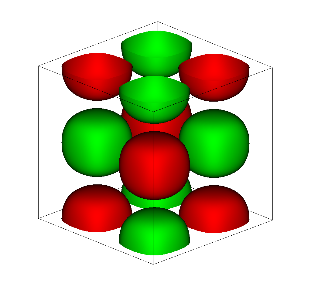
(a) Laminar flow at $t=0$ s.

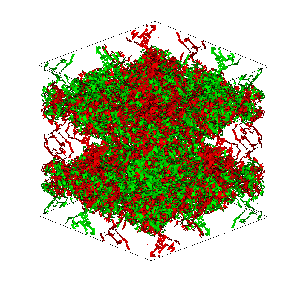
(b) Fully turbulent flow at $t=10$ s.

Figure 3: Taylor–Green vortex flow at $Re=1600$. Iso-surfaces of z-vorticity.

Due to the symmetric behavior of the flow, we are allowed to simulate only an eighth part of the domain. Hence, we take as computational domain $\Omega^{h}=\left[0,\pi\right]^{3}$ and apply no-penetration boundary conditions. All the implementations employ NURBS basis functions that are mostly $C^{1}$-quadratic, however every velocity space is enriched to be cubic $C^{2}$ in the associated direction [17, 18, 23, 24]. Note that conservation of angular momentum cannot be guaranteed, since the choice of the weighting function $\theta^{h}$ in section 5.3 is not valid. We apply a standard $L_{2}$-projection to set the initial condition on the mesh. For the time-integration we employ the generalized-$\alpha$ method with the parameter choices of [1] which yield correct energy evolution. This method is stable and shows second-order temporal accuracy. The resulting system of equations is solved with the standard flexible GMRES method with additive Schwartz preconditioning provided by Petsc [25, 26].

We perform simulations with three different methods: (i) the classical Galerkin method, (ii) the VMS method with static small-scales (VMSS), comparable with [8] and (iii) the novel Galerkin/least-squares formulation with dynamic and divergence-free small-scales (GLSDD), i.e. form (50). The DNS results of Brachet et al. [27] obtained with a spectral method on a fine $512^{3}$-mesh serve as reference data (ref).

First, we perform a brief mesh refinement study for the novel method. Figure 4 shows mesh refined results for the novel GLSDD method (50). For this purpose meshes with $16^{3}$, $24^{3}$, $32^{3}$, $48^{3}$ elements have been employed. Clearly, the energy behavior on the coarsest two meshes is quite off. The finer meshes are able to closely capture the turbulence character of the flow. In the following we therefore use meshes of $32^{3}$ or $48^{3}$ elements.

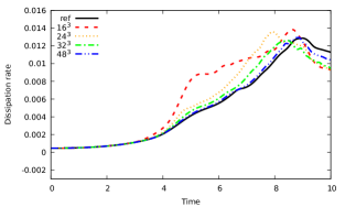
(a) Dissipation rate

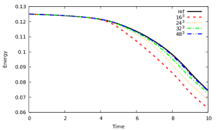
(b) Energy evolution

Figure 4: Taylor–Green vortex flow at $Re=1600$ mesh convergence. The GLS method with dynamic divergence-free small-scales.

We compare the results of the novel GLSDD method with the VMSS and the Galerkin approach. The simulations are carried out on a mesh of $32^{3}$ elements, i.e. the mesh size is $h=\frac{\pi}{32}$, and on a slightly finer mesh of $48^{3}$ elements. The time-step is taken as $\Delta t=\frac{4h}{5\pi}$, i.e. the initial CFL-number is roughly $0.25$. In the Figures 5-6 we visualize the time history of the kinetic energy and kinetic energy dissipation rate for each of the three methods and the reference data.

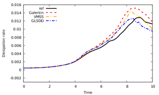
(a) Dissipation rate

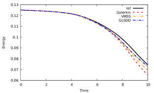
(b) Energy evolution

Figure 5: Taylor–Green vortex flow at $Re=1600$ on $32^{3}$-mesh for various methods: the Galerkin method, the VMS method with static small-scales and the GLS method with dynamic divergence-free small-scales.

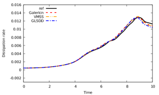
(a) Dissipation rate

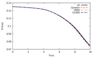
(b) Energy evolution

Figure 6: Taylor–Green vortex flow at $Re=1600$ on $48^{3}$-mesh for various methods: the Galerkin method, the VMS method with static small-scales and the GLS method with dynamic divergence-free small-scales.

The Figure 5 shows that each of the methods is able to roughly capture the energy behavior on the coarse mesh. The dissipation peek appears too early in time for each of the simulations. The Galerkin method displays the least accurate results, it overpredicts the dissipation rate. The VMSS method performs a bit better at all times. The novel GLSDD approach demonstrates an even closer agreement with the reference results. The results on the finer mesh, in Figure 6, reveal almost no difference with the reference data.

In the following we further analyze the contributions of the dissipation rate (on the course mesh). The dissipation rate of the Galerkin method only consists of the large-scale/physical dissipation $\|\nu^{1/2}\nabla\mathbf{u}^{h}\|_{\Omega}^{2}$. In contrast, the dissipation of the GLSDD method is composed of a large-scale and a small-scale contribution:

$$\dfrac{{\rm d}}{{\rm d}t}E_{\Omega}^{\text{GLSDD}}= -\|\nu^{1/2}\nabla\mathbf{u}^{h}\|_{\Omega}^{2}-\|\tau_{M}^{-1/2}\mathbf{u}^{\prime}\|_{\tilde{\Omega}}^{2}.$$ (67)

In Figure 7 we display the temporal evolution of both parts and the small-scale dissipation fraction
$(\|\tau_{M}^{-1/2}\mathbf{u}^{\prime}\|_{\tilde{\Omega}}^{2})/(\|\nu^{1/2}\nabla\mathbf{u}^{h}\|_{\Omega}^{2}+\|\tau_{M}^{-1/2}\mathbf{u}^{\prime}\|_{\tilde{\Omega}}^{2})$. In the laminar regime ($t<3$) the small-scale contribution is negligible. When the flow has a more turbulent character the contribution of the small-scales is substantial: the maximum of the dissipation fraction exceeds $0.35$.

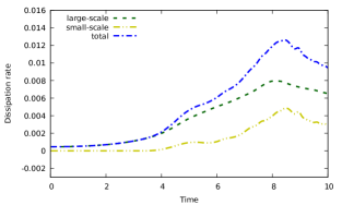
(a) Large- and small-scale contributions

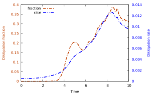
(b) The small-scale dissipation fraction

Figure 7: Taylor–Green vortex flow at $Re=1600$ on $32^{3}$-mesh with the GLSDD method: (a) large-scale and small-scale parts of the dissipation rate and (b) their fraction.

Lastly, we focus on the energy dissipation of the VMSS formulation. The derivation follows the same steps used throughout this paper. One might argue that the energy could also be solely based on the large-scales. This is what we do here. Its evolution reads:

$$\dfrac{{\rm d}}{{\rm d}t}E_{\Omega}^{h,\text{VMSS}}= -\|\nu^{1/2}\nabla\mathbf{u}^{h}\|_{\Omega}^{2}-\|\tau_{M}^{-1/2}\mathbf{u}^{\prime}\|_{\tilde{\Omega}}^{2}+(\nu\Delta\mathbf{u}^{h},\mathbf{u}^{\prime})_{\tilde{\Omega}}-\left(\mathbf{u}^{\prime},\partial_{t}\mathbf{u}^{h}\right)_{\tilde{\Omega}}$$

$$+(\nabla\cdot\mathbf{u}^{h},p^{\prime})_{\tilde{\Omega}}+\left(\nabla\mathbf{u}^{h},(\mathbf{u}^{h}+\mathbf{u}^{\prime})\otimes(\mathbf{u}^{h}+\mathbf{u}^{\prime})\right)_{\tilde{\Omega}}-\left(\mathbf{u}^{\prime},(\mathbf{u}^{h}+\mathbf{u}^{\prime})\cdot\nabla\mathbf{u}^{h}\right)_{\tilde{\Omega}}.$$ (68)

Figure 8 shows the contribution of the separate terms. The two desired dissipation terms are clearly dominant. The small-scale dissipation is smaller than the large-scale dissipation, however it has a significant contribution. Although the contributions are small, the unwanted terms can create artificial energy.

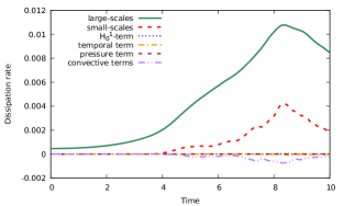
(a) All terms

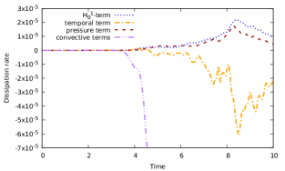
(b) Zoom unwanted terms

Figure 8: Taylor–Green vortex flow at $Re=1600$ on $32^{3}$-mesh with the VMSS method: energy dissipation of separate terms.

7 Conclusions

We continued the study initiated in [1] concerning the construction of methods displaying correct-energy behavior. In this paper we have applied the developed methodology to the incompressible Navier–Stokes equations. It clearly shows that the link between the methods VMS, SUPG and GLS, established in [1], is also valid for the incompressible Navier–Stokes equations.

The novel GLSDD methodology employs divergence-conforming NURBS basis functions and uses a Lagrange multiplier setting to ensure divergence-free small-scales. Furthermore, it enjoys the favorable behavior of the dynamic small-scales and reduces to the Galerkin method in the Stokes regime. These properties all emerge from the correct-energy design condition. A pleasant byproduct of the method is the conservation of linear momentum. The conservation of angular momentum can be achieved when employing the appropriate weighting function spaces. The numerical results support the theoretical framework in that the energy behavior improves upon the VMS method with static small-scales. The variational multiscale method with static small-scales has unwanted small-scale contributions which create artificial energy.

The novel formulation requires a bit more effort to implement compared to the variational multiscale method with static small-scales. One has to include an additional variable to ensure the divergence-free behavior of the small-scales. In addition the formulation needs to be equipped with the dynamic small-scale model. However, the resulting system of equations does not demand a sophisticated preconditioner; we have employed the standard ASM (Additive Schwarz Method) technique. In our opinion, the accuracy gain outweighs the little extra implementation effort and calculation cost.

We see several directions for future work. The first concerns the development of a method displaying correct energy behavior at the boundary, in particular when using the weak imposition of Dirichlet boundary conditions. This allows to test the effect of correct energy behavior on wall-bounded turbulent flow problems. Another extension is correct energy behavior for free-surface flow computations. This is an important step, since artificial energy creation can yield highly instable behavior, as demonstrated in [28]. We have work on both extensions in progress and aim to report on it in the near future.

Appendix A Galerkin/least-squares formulation with dynamic divergence-free small-scales

We repeat the Galerkin/least-squares formulation with dynamic divergence-free small-scales (GLSDD), i.e. form (50), to provide an overview of the separate terms. The formulation is of skew-symmetric type, applies GLS stabilization and uses divergence-free dynamic small-scales. The method requires a stable velocity–pressure pair and reads:

Find $\left(\mathbf{u}^{h},p^{h},\zeta^{h}\right)\in\mathcal{W}^{h}\times\mathcal{P}^{h}$ such that for all $\left(\mathbf{w}^{h},q^{h},\theta^{h}\right)\in\mathcal{W}^{h}\times\mathcal{P}^{h}$,

$$\begin{split}\left(\mathbf{w}^{h},\partial_{t}\mathbf{u}^{h}\right)_{\Omega}+{}&\left(\mathbf{w}^{h},\partial_{t}\mathbf{u}^{\prime}\right)_{\tilde{\Omega}}\\[6.0pt] +&\tfrac{1}{2}(\mathbf{w}^{h},(\mathbf{u}^{h}+\mathbf{u}^{\prime})\cdot\nabla\mathbf{u}^{h})_{\Omega}-\tfrac{1}{2}((\mathbf{u}^{h}+\mathbf{u}^{\prime})\cdot\nabla\mathbf{w}^{h},\mathbf{u}^{h})_{\Omega}-\left(\left(\mathbf{u}^{h}+\mathbf{u}^{\prime}\right)\cdot\nabla\mathbf{w}^{h},\mathbf{u}^{\prime}\right)_{\tilde{\Omega}}\\[6.0pt] +&(\nabla\mathbf{w}^{h},2\nu\nabla^{s}\mathbf{u}^{h})_{\Omega}+\left(\nu\Delta\mathbf{w}^{h},\mathbf{u}^{\prime}\right)_{\tilde{\Omega}}\\[6.0pt] +&(q^{h},\nabla\cdot\mathbf{u}^{h})_{\Omega}-(\nabla\cdot\mathbf{w}^{h},p^{h})_{\Omega}+\left(\nabla\theta^{h},\mathbf{u}^{\prime}\right)_{\tilde{\Omega}}=(\mathbf{w},\mathbf{f})_{\Omega},\end{split}$$ (69a)

$$\begin{split}\partial_{t}\mathbf{u}^{\prime}+\tau_{M}^{-1}\mathbf{u}^{\prime}+\nabla\zeta^{h}{}&+\mbox{\boldmath{$r$}}_{M}=0,\end{split}$$ (69b)

where momentum residual is

$$\mbox{\boldmath{$r$}}_{M}=\partial_{t}\mathbf{u}^{h}+\left(\left(\mathbf{u}^{h}+\mathbf{u}^{\prime}\right)\cdot\nabla\right)\mathbf{u}^{h}+\nabla p^{h}-\nu\Delta\mathbf{u}^{h}-\mathbf{f}.$$ (70)

The separate terms of (69a) are from left to right: the temporal terms, the convective contributions, the viscous contributions, the incompressibility constraint, the pressure term, the divergence-free small-scale velocity constraint and the forcing term. This form follows the correct-energy evolution (on a local scale):

$$\dfrac{{\rm d}}{{\rm d}t}E_{\omega}= -\|\nu^{1/2}\nabla\mathbf{u}^{h}\|_{\omega}^{2}+(\mathbf{u}^{h},\mathbf{f})_{\omega}-(1,F_{\omega}^{h})_{\chi_{\omega}}$$

$$-\|\tau_{M}^{-1/2}\mathbf{u}^{\prime}\|_{\tilde{\omega}}^{2}+(\mathbf{u}^{\prime},\mathbf{f})_{\tilde{\omega}},$$ (71)

and possesses the conservation properties of Section 5.

Appendix B Definition dynamic stabilization parameter

The dynamic stabilization parameter $\tau_{M}$ is the discrete approximation of the inverse of the convective and viscous parts of momentum Navier–Stokes operator. It mirrors the dynamic stabilization parameter of convection–diffusion equation (see [1]). The continuity stabilization parameter $\tau_{C}$ is on its turn the discrete approximation of the inverse of the divergence operator, here we use the objective definition introduced in [22]. The parameters take the form:

$$\tau_{M}= \left(\tau^{-2}_{\text{conv}}+\tau^{-2}_{\text{visc}}\right)^{-1/2},$$ (72a)

$$\tau_{C}= \left(\tau_{M}\sqrt{\mathbf{G}:\mathbf{G}}\right)^{-1},$$ (72b)

where the convective and viscous contributions of $\tau_{M}$ are

$$\tau_{\text{conv}}^{-2}= 4\mathbf{u}\cdot\mathbf{G}\mathbf{u},$$ (73a)

$$\tau_{\text{visc}}^{-2}= C_{I}\nu^{2}\mathbf{G}:\mathbf{G}.$$ (73b)

Here the following definition is employed:

$$\mathbf{G} =\frac{\partial\boldsymbol{\xi}}{\partial\mbox{\boldmath{$x$}}}^{T}\frac{\partial\boldsymbol{\xi}}{\partial\mbox{\boldmath{$x$}}},$$ (74a)

$$\mathbf{G}:\mathbf{G} =\displaystyle\sum_{i,j=1}^{3}G_{ij}G_{ij},$$ (74b)

where $\partial\boldsymbol{\xi}/\partial\mbox{\boldmath{$x$}}$ is the inverse Jacobian of the map between the elements in the reference and physical domain. The positive constant $C_{I}$ is determined by an inverse estimate.

References

- [1] M.F.P. ten Eikelder and I. Akkerman. Correct energy evolution of stabilized formulations: The relation between VMS, SUPG and GLS via dynamic orthogonal small-scales and isogeometric analysis. I: The convective–diffusive context. Computer Methods in Applied Mechanics and Engineering, 331:259–280, 2018.
- [2] I. Akkerman and M.F.P. ten Eikelder. Toward free-surface flow simulations with correct energy evolution: an isogeometric level-set approach with monolithic time-integration. arXiv preprint arXiv:1801.08759, 2018.
- [3] T.J.R. Hughes and G.N. Wells. Conservation properties for the Galerkin and stabilised forms of the advection-diffusion and incompressible Navier-Stokes equations. Computer Methods in Applied Mechanics and Engineering, 194:1141–1159, 2005.
- [4] R. Codina. Stabilized finite element approximation of transient incompressible flows using orthogonal subscales. Computer Methods in Applied Mechanics and Engineering, 191:4295–4321, 2002.
- [5] R. Codina, J. Principe, O. Guasch, and S. Badia. Time dependent subscales in the stabilized finite element approximation of incompressible flow problems. Computer Methods in Applied Mechanics and Engineering, 196:2413–2430, 2007.
- [6] T. J. R. Hughes. Multiscale phenomena: Green’s functions, the Dirichlet-to-Neumann formulation, subgrid scale models, bubbles and the origins of stabilized methods. Computer Methods in Applied Mechanics and Engineering, 127:387–401, 1995.
- [7] T. J. R. Hughes, G. Feijóo., L. Mazzei, and J. B. Quincy. The variational multiscale method – A paradigm for computational mechanics. Computer Methods in Applied Mechanics and Engineering, 166:3–24, 1998.
- [8] Y. Bazilevs, V.M. Calo, J.A. Cottrel, T. J. R. Hughes, A. Reali, and G. Scovazzi. Variational multiscale residual-based turbulence modeling for large eddy simulation of incompressible flows. Computer Methods in Applied Mechanics and Engineering, 197:173–201, 2007.
- [9] R. Codina, S. Badia, J. Baiges, and J. Principe. Variational multiscale methods in computational fluid dynamics. Encyclopedia of computational mechanics, E. Stein, R. de Borst, and TJ Hughes, Eds., Wiley Online Library, 2017.
- [10] Z. Wang and A.A. Oberai. Spectral analysis of the dissipation of the residual-based variational multiscale method. Computer Methods in Applied Mechanics and Engineering, 199:810–818, 2010.
- [11] J. Principe, R. Codina, and F. Henke. The dissipative structure of variational multiscale methods for incompressible flows. Computer Methods in Applied Mechanics and Engineering, 199:791–801, 2010.
- [12] O. Colomés, S. Badia, R. Codina, and J. Principe. Assessment of variational multiscale models for the large eddy simulation of turbulent incompressible flows. Computer Methods in Applied Mechanics and Engineering, 285:32–63, 2015.
- [13] T.M. Opstal, J. Yan, J.A. Evans, T. Kvamsdal, and Y. Bazilevs. Isogeometric divergence-conforming variational multiscale formulation of incompressible turbulent flows. Computer Methods in Applied Mechanics and Engineering, 361:859–879, 2017.
- [14] T. J. R. Hughes, J.A. Cottrell, and Y. Bazilevs. Isogeometric analysis: CAD, finite elements, NURBS, exact geometry, and mesh refinement. Computer Methods in Applied Mechanics and Engineering, 194:4135–4195, 2005.
- [15] S. Lipton, J. Evans, Y. Bazilevs, T. Elguedj, and T. J. R. Hughes. Robustness of isogeometric structural discretizations under severe mesh distortion. Computer Methods in Applied Mechanics and Engineering, 199:357–373, 2009.
- [16] I. Akkerman, Y. Bazilevs, V.M. Calo, T. J. R. Hughes, and S. Hulshoff. The role of continuity in residual-based variational multiscale modeling of turbulence. Computational Mechanics, 41:371–378, 2008.
- [17] J.A. Evans and T. J. R. Hughes. Isogeometric divergence-conforming B-splines for the steady Navier–Stokes equations. Mathematical Models and Methods in Applied Sciences, 23:1421–1478, 2013.
- [18] J.A. Evans and T. J. R. Hughes. Isogeometric divergence-conforming B-splines for the unsteady Navier–Stokes equations. Journal of Computational Physics, 241:141–167, 2013.
- [19] T. J. R. Hughes, G. Engel, L. Mazzei, and M. Larson. The Continuous Galerkin Method is Locally Conservative. Journal of Computational Physics, 163:467–488, 2000.
- [20] T. J. R. Hughes and G. Sangalli. Variational multiscale analysis: the fine-scale Green’s function, projection, optimization, localization, and stabilized methods. SIAM Journal of Numerical Analysis, 45:539–557, 2007.
- [21] J. Chung and G. M. Hulbert. A time integration algorithm for structural dynamics with improved numerical dissipation: The generalized- method. Journal of Applied Mechanics, 60:371–75, 1993.
- [22] Y. Bazilevs and I. Akkerman. Large eddy simulation of turbulent Taylor–Couette flow using isogeometric analysis and the residual-based variational multiscale method. Journal of Computational Physics, 229:3402 – 3414, 2010.
- [23] A. Buffa, C. De Falco, and G. Sangalli. IsoGeometric Analysis: Stable elements for the 2D Stokes equation. International Journal for Numerical Methods in Fluids, 65:1407–1422, 2011.
- [24] A. Buffa, J. Rivas, G. Sangalli, and R. Vázquez. Isogeometric Discrete Differential Forms in Three Dimensions. SIAM Journal on Numerical Analysis, 49:818–844, 2011.
- [25] S. Balay, W. Gropp, L. C. McInnes, and B. Smith. PETSc 2.0 users manual. Mathematics and Computer Science Division, Argonne National Laboratory http://www.mcs.anl.gov/petsc, 2000.
- [26] S. Balay, W.D. Gropp, L.C. McInnes, and B.F. Smith. Efficient management of parallelism in object oriented numerical software libraries. In E. Arge, A. M. Bruaset, and H. P. Langtangen, editors, Modern Software Tools in Scientific Computing, pages 163–202. Birkhäuser Press, 1997.
- [27] M.E. Brachet, D.I. Meiron, S.A. Orszag, B.G. Nickel, R.H. Morf, and U. Frisch. Small-scale structure of the Taylor–Green vortex. Journal of Fluid Mechanics, 130:411–452, 1983.
- [28] I. Akkerman, Y. Bazilevs, D.J. Benson, M.W. Farthing, and C.E. Kees. Free-Surface Flow and Fluid-Object Interaction Modeling With Emphasis on Ship Hydrodynamics. Journal of Applied Mechanics, 79: 010905, 2012.