A fully discrete approximation of the one-dimensional stochastic heat equation

Abstract

A fully discrete approximation of the one-dimensional stochastic heat equation driven by multiplicative space-time white noise is presented. The standard finite difference approximation is used in space and a stochastic exponential method is used for the temporal approximation. Observe that the proposed exponential scheme does not suffer from any kind of CFL-type step size restriction. When the drift term and the diffusion coefficient are assumed to be globally Lipschitz, this explicit time integrator allows for error bounds in $L^{q}(\Omega)$, for all $q\geq 2$, improving some existing results in the literature. On top of this, we also prove almost sure convergence of the numerical scheme. In the case of non-globally Lipschitz coefficients, we provide sufficient conditions under which the numerical solution converges in probability to the exact solution. Numerical experiments are presented to illustrate the theoretical results.
Mathematics Subject Classification (2010): 60H15; 60H35.
Keywords:stochastic heat equation; multiplicative noise; finite difference scheme; stochastic exponential integrator; $L^{q}(\Omega)$-convergence.

1 Introduction

We study an explicit full numerical discretization of the one-dimensional stochastic heat equation

$$\frac{\partial}{\partial t}u(t,x)=\frac{\partial^{2}}{\partial x^{2}}u(t,x)+f(t,x,u(t,x))+\sigma(t,x,u(t,x))\frac{\partial^{2}}{\partial t\partial x}W(t,x)\quad\mathrm{in}\>\ (0,\infty)\times(0,1),$$

$$u(t,0)=u(t,1)=0\quad\mathrm{for}\>\ t\in(0,\infty),$$

$$u(0,x)=u_{0}\quad\mathrm{for}\>\ x\in[0,1],$$ (1)

where $W$ is a Brownian sheet on $[0,\infty)\times[0,1]$ defined on some probability space $(\Omega,\mathcal{F},\mathbb{P})$ satisfying the usual conditions, and $u_{0}$ is a continuous function in $[0,1]$ such that $u_{0}(0)=u_{0}(1)=0$. Assumptions on the coefficients $f$ and $\sigma$ will be specified below. As far as the spatial discretization is concerned, we use a standard finite difference scheme, as in [20]. In order to discretize (1) with respect to the time variable, we consider an exponential method similar to the time integrators used in [9, 10, 3] for stochastic wave equations or in [2, 8] for stochastic Schrödinger equations.

Our main aim is to improve the temporal rate of convergence that has been obtained by Gyöngy in the reference [21]. Indeed, in [21], the explicit as well as the semi-implicit Euler-Maruyama scheme have been applied for the time discretization of problem (1). When the functions $f$ and $\sigma$ are globally Lipschitz continuous in the third variable, a temporal convergence order of $\frac{1}{8}-$ in the $L^{q}(\Omega)$-norm, for all $q\geq 2$, is obtained for these numerical schemes (see Theorem 3.1 in [21] for a precise statement). Our first objective is to see if an explicit exponential method can provide a higher rate of convergence. In the present work, we answer this question positively and obtain the temporal rate $\frac{1}{4}-$ (see the first part of Theorem 2.3 below). We note that, as in [21], the latter estimate for the $L^{q}(\Omega)$-error holds for any fixed $t\in(0,T]$ and uniformly in the spatial variable, where $T>0$ is some fixed time horizon. On the other hand, we should also remark that, in [21], a rate of convergence $\frac{1}{4}$ could be obtained only in the case where the initial condition $u_{0}$ belongs to $C^{3}([0,1])$. Finally, as in [21], we also prove that the exponential scheme converges almost surely to the solution of (1), uniformly with respect to time and space variables (cf. Theorem 2.4).

Our second objective consists in refining the above-mentioned temporal rate of convergence in order to end up with a convergence order which is exactly $\frac{1}{4}$ and with an estimate which is uniform both with respect to time and space variables. To this end, we assume that the initial condition $u_{0}$ belongs to some fractional Sobolev space (see (12) for the precise definition). Indeed, as it can be deduced from the second part of Theorem 2.3 and well-known Sobolev embedding results, in order to have the rate $\frac{1}{4}$, the hypothesis on $u_{0}$ implies that it is $\delta$-Hölder continuous for all $\delta\in(0,\frac{1}{2})$. Eventually, as in [21], we remove the globally Lipschitz assumption on the coefficients $f$ and $\sigma$ in equation (1), and we prove convergence in probability for the proposed explicit exponential integrator (see Theorem 3.1 below).

We should point out that there are also other important advantages with using the exponential method proposed here. Namely, first, it does not suffer a step size restriction (imposed by a CFL condition) as the explicit Euler-Maruyama scheme from [21]. Secondly, it is an explicit scheme and therefore has implementation advantages over the implicit Euler-Maruyama scheme studied in [21]. These facts will be illustrated numerically.

The numerical analysis of the stochastic heat equation (1) is an active research area. Without being too exhaustive, beside the above mentioned papers [20] and [21], we mention the following works regarding numerical discretizations of stochastic parabolic partial differential equations: [20, 55, 5, 47] (spatial approximations); [18, 22, 23, 1, 48, 45, 15, 17, 26, 44, 52, 39, 40, 31, 28, 11, 30, 29, 34, 38, 54, 6, 12, 33, 7, 53] (temporal and full discretizations); [49, 36] (stability). Observe that most of these references are concerned with an interpretation of stochastic partial differential equations in Hilbert spaces and thus error estimates are provided in the $L^{2}([0,1])$ norm (or similar norms). The reader is referred to the monographs [32, 35, 37] for a more comprehensive reference list.

In the present publication, we follow a similar approach as in [10] and [21]. The main idea consists in establishing suitable mild forms for the spatial approximation $u^{M}$ and for the fully discretization scheme $u^{M,N}$. The obtained mild equations, together with some auxiliary results and taking into account the hypotheses on the coefficients and initial data, will allow us to deal with the $L^{q}(\Omega)$-error

$$\Bigl{(}\mathbb{E}[|u^{M}(t,x)-u^{M,N}(t,x)|^{q}]\Bigr{)}^{\frac{1}{q}},$$

for all $q\geq 2$. The $L^{q}(\Omega)$-error comparing $u^{M}$ with the exact solution of (1) has already been studied in [20].

The paper is organized as follows. In Section 2, we study the numerical approximation of the solution to equation (1) in the case of globally Lipschitz continuous coefficients. More precisely, we first recall the spatial discretization $u^{M}$ of (1) and prove some properties of $u^{M}$ needed in the sequel. Next, we introduce the full discretization scheme and prove that it satisfies a suitable mild form, and provide three auxiliary results which will be invoked in the convergence results’ proofs. At this point, we state and prove the main result on $L^{q}(\Omega)$-convergence along with some numerical experiments illustrating its conclusion. Section 2 concludes with the result on almost sure convergence, where we also provide some numerical experiments. Finally, Section 3 is devoted to deal with the convergence in probability of the numerical solution to the exact solution of (1), in the case where the coefficients $f$ and $\sigma$ are non-globally Lipschitz continuous.

Observe that, throughout this article, $C$ will denote a generic constant that may vary from line to line.

2 Error analysis for globally Lipschitz continuous coefficients

This section is divided into three subsections. We begin by stating the assumptions we will make and by recalling the mild solution of (1). The first subsection is dedicated to recalling the finite difference approximation from [20] and some (new) results about it. In the second subsection, we numerically integrate the resulting semi-discrete system of stochastic differential equations in time to obtain a full approximation of (1). We also state and prove our main result about convergence in the $2p$-th mean. Finally, in the third subsection, we prove almost sure convergence of the full approximation to the exact solution. In addition, numerical experiments are provided to illustrate the theoretical results of this section.

In this section, we shall make the following assumptions on the coefficients of the stochastic heat equation (1): for a given positive real number $T$, there exist a constant $C$ such that

$$|f(t,x,u)-f(t,y,v)|+|\sigma(t,x,u)-\sigma(t,y,v)|\leq C\bigl{(}|x-y|+|u-v|\bigr{)},$$ (L)

for all $t\in[0,T]$, $x,y\in[0,1]$, $u,v\in\mathbb{R}$, and

$$|f(t,x,u)|+|\sigma(t,x,u)|\leq C(1+|u|),$$ (LG)

for all $t\in[0,T]$, $x\in[0,1]$, $u\in\mathbb{R}$. Assume also that the initial condition $u_{0}$ defines a continuous function on $[0,1]$ with $u_{0}(0)=u_{0}(1)=0$. The assumptions (L) and (LG) imply existence and uniqueness of a solution $u$ of equation (1) on the time interval $[0,T]$, see e.g. Theorem 3.2 and Exercise 3.4 in [51]. Let us recall that, for a stochastic basis $(\Omega,\mathcal{F},(\mathcal{F}_{t})_{t\geq 0},\mathbb{P})$, a solution to equation (1) is an $\mathcal{F}_{t}$-adapted continuous process $\{u(t,x),(t,x)\in[0,T]\times[0,1]\}$ satisfying that, for every $\Phi\in C^{\infty}(\mathbb{R}^{2})$ such that $\Phi(t,0)=\Phi(t,1)=0$ for all $t\geq 0$, we have

$$\int_{0}^{1}u(t,x)\Phi(t,x)\,\mathrm{d}x= \int_{0}^{1}u_{0}(x)\Phi(t,x)\,\mathrm{d}x$$

$$\quad+\int_{0}^{t}\int_{0}^{1}u(s,x)\left(\frac{\partial^{2}\Phi}{\partial x^{2}}(s,x)+\frac{\partial\Phi}{\partial s}(s,x)\right)\,\mathrm{d}x\,\mathrm{d}s$$

$$\quad+\int_{0}^{t}\int_{0}^{1}f(s,x,u(s,x))\Phi(s,x)\,\mathrm{d}x\,\mathrm{d}s$$

$$\quad+\int_{0}^{t}\int_{0}^{1}\sigma(s,x,u(s,x))\Phi(s,x)\,W(\mathrm{d}s,\mathrm{d}x),\quad\mathbb{P}\text{-a.s.},$$ (2)

for all $t\in[0,T]$. It is well-known that the above equation implies the following mild form for (1):

$$u(t,x) =\int_{0}^{1}G(t,x,y)u_{0}(y)\,\mathrm{d}y+\int_{0}^{t}\int_{0}^{1}G(t-s,x,y)f(s,y,u(s,y))\,\mathrm{d}y\,\mathrm{d}s$$ (3)

$$\quad+\int_{0}^{t}\int_{0}^{1}G(t-s,x,y)\sigma(s,y,u(s,y))\,W(\mathrm{d}s,\mathrm{d}y),\quad\mathbb{P}\text{-a.s.},$$

where $G(t,x,y)$ is the Green function of the linear heat equation with homogeneous Dirichlet boundary conditions:

$$G(t,x,y)=\sum_{j=1}^{\infty}e^{-j^{2}\pi^{2}t}\varphi_{j}(x)\varphi_{j}(y),\quad t>0,\,x,y\in[0,1],$$

with $\varphi_{j}(x):=\sqrt{2}\sin(j\pi x)$, $j\geq 1$. Note that these functions form an orthonormal basis of $L^{2}([0,1])$.

2.1 Spatial discretization of the stochastic heat equation

In this subsection we recall the finite difference discretization and some results obtained in [20]. In addition to this, we show new regularity results for the approximated Green function $G^{M}(t,x,y)$ defined below, and for the space discrete approximation, which will be needed in the sequel.

Let $M\geq 1$ be an integer and define the grid points $x_{m}=\frac{m}{M}$ for $m=0,\ldots,M$, and the mesh size $\Delta x=\frac{1}{M}$. We now use the standard finite difference scheme for the spatial approximation of (1) from [20]. Let the process $u^{M}(t,\cdot)$ be defined as the solution of the system of stochastic differential equations (for $m=1,\ldots,M-1$)

$$\text{d}u^{M}(t,x_{m}) =M^{2}\left(u^{M}(t,x_{m+1})-2u^{M}(t,x_{m})+u^{M}(t,x_{m-1})\right)\,\mathrm{d}t$$ (4)

$$\quad+f(t,x_{m},u^{M}(t,x_{m}))\,\mathrm{d}t$$

$$\quad+M\sigma(t,x_{m},u^{M}(t,x_{m}))\,\mathrm{d}(W(t,x_{m+1})-W(t,x_{m}))$$

with Dirichlet boundary conditions

$$u^{M}(t,0)=u^{M}(t,1)=0,$$

and initial value

$$u^{M}(0,x_{m})=u_{0}(x_{m}),$$

for $m=1,\ldots,M-1$. For $x\in[x_{m},x_{m+1})$ we define

$$u^{M}(t,x):=u^{M}(t,x_{m})+(Mx-m)(u^{M}(t,x_{m+1})-u^{M}(t,x_{m})).$$ (5)

We use the notations $u_{m}^{M}(t):=u^{M}(t,x_{m})$ and $W_{m}^{M}(t):=\sqrt{M}(W(t,x_{m+1})-W(t,x_{m}))$, for $m=1,\ldots,M-1$ and write the system (4) as

$$\text{d}u^{M}_{m}(t) =M^{2}\sum_{i=1}^{M-1}D_{mi}u^{M}_{i}(t)\,\mathrm{d}t+f(t,x_{m},u^{M}_{m}(t))\,\mathrm{d}t$$

$$\quad+\sqrt{M}\sigma(t,x_{m},u^{M}_{m}(t))\,\mathrm{d}W_{m}^{M}(t),$$

with initial value

$$u_{m}^{M}(0)=u_{0}(x_{m}),$$

for $m=1,\ldots,M-1,$ where $D=(D_{mi})_{m,i}$ is a square matrix of size $M-1$, with elements $D_{mm}=-2$, $D_{mi}=1$ for $|m-i|=1$, $D_{mi}=0$ for $|m-i|>1$. Also $W^{M}(t):=(W^{M}_{m}(t))_{m=1}^{M-1}$ is an $M-1$ dimensional Wiener process. Observe that the matrix $M^{2}D$ has eigenvalues

$$\lambda_{j}^{M}:=-4\sin^{2}\left(\frac{j\pi}{2M}\right)M^{2}=-j^{2}\pi^{2}c_{j}^{M},$$

where

$$\frac{4}{\pi^{2}}\leq c_{j}^{M}:=\frac{\sin^{2}\left(\frac{j\pi}{2M}\right)}{\left(\frac{j\pi}{2M}\right)^{2}}\leq 1,$$

for $j=1,2,\ldots,M-1$ and every $M\geq 1$.

Using the variation of constants formula, the exact solution to (4) reads

$$u^{M}(t,x_{m}) =\frac{1}{M}\sum_{l=1}^{M-1}\sum_{j=1}^{M-1}\exp(\lambda_{j}^{M}t)\varphi_{j}(x_{m})\varphi_{j}(x_{l})u_{0}(x_{l})$$ (6)

$$\quad+\int_{0}^{t}\frac{1}{M}\sum_{l=1}^{M-1}\sum_{j=1}^{M-1}\exp(\lambda_{j}^{M}(t-s))\varphi_{j}(x_{m})\varphi_{j}(x_{l})f(s,x_{l},u^{M}(s,x_{l}))\,\mathrm{d}s$$

$$\quad+\int_{0}^{t}\frac{1}{\sqrt{M}}\sum_{l=1}^{M-1}\sum_{j=1}^{M-1}\exp(\lambda_{j}^{M}(t-s))\varphi_{j}(x_{m})\varphi_{j}(x_{l})\sigma(s,x_{l},u^{M}(s,x_{l}))\,\mathrm{d}W_{l}^{M}(s),$$

where we recall that $\varphi_{j}(x):=\sqrt{2}\sin(jx\pi)$ for $j=1,\ldots,M-1$.

We next define the discrete kernel $G^{M}(t,x,y)$ by

$$G^{M}(t,x,y):=\sum_{j=1}^{M-1}\exp(\lambda_{j}^{M}t)\varphi_{j}^{M}(x)\varphi_{j}(\kappa_{M}(y)),$$ (7)

where $\kappa_{M}(y):=\frac{[My]}{M}$, $\varphi_{j}^{M}(x):=\varphi_{j}(x_{l})$ for $x=x_{l}$ and

$$\varphi_{j}^{M}(x):=\varphi_{j}(x_{l})+(Mx-l)\left(\varphi_{j}(x_{l+1})-\varphi_{j}(x_{l})\right),\quad\text{if }x\in(x_{l},x_{l+1}].$$

With these definitions in hand, one sees that the semi-discrete solution $u^{M}$ satisfies the mild equation:

$$u^{M}(t,x) =\int_{0}^{1}G^{M}(t,x,y)u_{0}(\kappa_{M}(y))\,\mathrm{d}y$$ (8)

$$\quad+\int_{0}^{t}\int_{0}^{1}G^{M}(t-s,x,y)f(s,\kappa_{M}(y),u^{M}(s,\kappa_{M}(y)))\,\mathrm{d}y\,\mathrm{d}s$$

$$\quad+\int_{0}^{t}\int_{0}^{1}G^{M}(t-s,x,y)\sigma(s,\kappa_{M}(y),u^{M}(s,\kappa_{M}(y)))\,\mathrm{d}W(s,y)$$

$\mathbb{P}$-a.s., for all $t\geq 0$ and $x\in[0,1].$

Next, we proceed by collecting some useful results for the error analysis of the fully discrete numerical discretization presented in the next subsection. The following two results are proved in [20]. Recall that $u^{M}$ is the space discrete approximation given by (8) and that $u$ is the exact solution given by equation (3).

Proposition 2.1 (Proposition $3.5$ in [20]).

Assume that $u_{0}\in C([0,1])$ with $u_{0}(0)=u_{0}(1)=0$, and that the functions $f$ and $\sigma$ satisfy the condition (LG). Then, for every $p\geq 1$, there exists a constant $C$ such that

$$\sup_{M\geq 1}\sup_{(t,x)\in[0,T]\times[0,1]}\mathbb{E}[|u^{M}(t,x)|^{2p}]\leq C.$$

Theorem 2.1 (Theorem $3.1$ in [20]).

Assume that $f$ and $\sigma$ satisfy the conditions (L) and (LG), and that $u_{0}\in C([0,1])$ with $u_{0}(0)=u_{0}(1)=0$. Then, for every $0<\alpha<\frac{1}{4}$, $p\geq 1$ and for every $t>0$, there is a constant $C=C(\alpha,p,t)$ such that

$$\sup_{x\in[0,1]}\Big{(}\mathbb{E}[|u^{M}(t,x)-u(t,x)|^{2p}]\Big{)}^{\frac{1}{2p}}\leq C(\Delta x)^{\alpha}.$$ (9)

We recall that $\Delta x=1/M$ is the mesh size in space. Moreover, $u^{M}(t,x)$ converges to $u(t,x)$ almost surely as $M\rightarrow\infty$, uniformly in $t\in[0,T]$ and $x\in[0,1]$, for every $T>0$.

If $u_{0}$ is sufficiently smooth (e.g. $u_{0}\in C^{3}([0,1])$) then for every $T>0$, estimate (9) holds with $\alpha=\frac{1}{2}$ and with the same constant $C$ for all $t\in[0,T]$ and integer $M\geq 1$.

We will also make use of the following estimates on the discrete Green function.

Lemma 2.1.

There is a constant $C$ such that the following estimates hold:

1. For all $0<s<t\leq T$:

   $$\sup_{M\geq 1}\sup_{x\in[0,1]}\int_{0}^{s}\int_{0}^{1}|G^{M}(t-r,x,y)-G^{M}(s-r,x,y)|^{2}\,\mathrm{d}y\,\mathrm{d}r\leq C(t-s)^{1/2}.$$ (10)

2. For all $t\in(0,T]$:

   $$\sup_{M\geq 1}\sup_{x\in[0,1]}\int_{0}^{1}|G^{M}(t,x,y)|^{2}\,\mathrm{d}y\leq C\frac{1}{\sqrt{t}}.$$

3. For all $0<s<t\leq T$ and $\alpha\in(\frac{1}{2},\frac{5}{2})$:

   $$\sup_{M\geq 1}\sup_{x\in[0,1]}\int_{0}^{1}|G^{M}(t,x,y)-G^{M}(s,x,y)|^{2}\,\mathrm{d}y\leq Cs^{-\alpha}(t-s)^{\alpha-\frac{1}{2}}.$$

Proof.

Recall that

$$G^{M}(t,x,y)=\sum_{j=1}^{M-1}\exp(\lambda_{j}^{M}t)\varphi_{j}^{M}(x)\varphi_{j}(\kappa_{M}(y)),$$

where $\kappa_{M}(y)=\frac{[My]}{M},$ $\varphi_{j}^{M}(x)=\varphi_{j}\left(\frac{l}{M}\right)$ for $x=\frac{l}{M}$ and

$$\varphi_{j}^{M}(x)=\varphi_{j}\left(\frac{l}{M}\right)+(Mx-l)\left(\varphi_{j}\left(\frac{l+1}{M}\right)-\varphi_{j}\left(\frac{l}{M}\right)\right),\quad\text{if }x\in\left(\frac{l}{M},\frac{l+1}{M}\right].$$

We first prove $(i)$. Observe that a general version of this result is used in the proof of [20, Lem. 3.6] (see the term $A_{1}^{2p}$ therein). Using the definition of the discrete Green function, we have

$$\int_{0}^{s}\int_{0}^{1}|G^{M}(t-r,x,y)-G^{M}(s-r,x,y)|^{2}\,\mathrm{d}y\,\mathrm{d}r$$

$$\quad=\int_{0}^{s}\int_{0}^{1}\left|\sum_{j=1}^{M-1}(\exp(\lambda_{j}^{M}(t-r))-\exp(\lambda_{j}^{M}(s-r)))\varphi_{j}^{M}(x)\varphi_{j}(\kappa_{M}(y))\right|^{2}\,\mathrm{d}y\,\mathrm{d}r.$$

At this point, we use the fact that the vectors

$$e_{j}=\left(\sqrt{\frac{2}{M}}\sin\left(j\frac{k}{M}\pi\right),\;k=1,\dots,M-1\right),\quad j=1,\dots,M-1,$$

form an orthonormal basis of $\mathbb{R}^{M-1}$, which implies that

$$\int_{0}^{1}\varphi_{j}(\kappa_{M}(y))\varphi_{l}(\kappa_{M}(y))\,\mathrm{d}y=\delta_{\{j=l\}}.$$ (11)

Hence, using also the definitions of $\varphi_{j}^{M}$ and $\lambda_{j}^{M}$,

$$\int_{0}^{s}\int_{0}^{1}|G^{M}(t-r,x,y)-G^{M}(s-r,x,y)|^{2}\,\mathrm{d}y\,\mathrm{d}r$$

$$\quad=\int_{0}^{s}\sum_{j=1}^{M-1}|\exp(\lambda_{j}^{M}(t-r)-\exp(\lambda_{j}^{M}(s-r))|^{2}|\varphi_{j}^{M}(x)|^{2}\,\mathrm{d}r$$

$$\quad\leq C\sum_{j=1}^{M-1}\int_{0}^{s}\exp(\lambda_{j}^{M}(s-r))^{2}\,\mathrm{d}r|1-\exp(\lambda_{j}^{M}(t-s))|^{2}$$

$$\quad\leq C\sum_{j=1}^{M-1}\int_{0}^{s}\exp(-2j^{2}\pi^{2}c_{j}^{M}(s-r))\,\mathrm{d}r(1-\exp(-j^{2}\pi^{2}c_{j}^{M}(t-s)))^{2}$$

$$\quad\leq C\sum_{j=1}^{\infty}j^{-2}(j^{4}(t-s)^{2}\wedge 1).$$

Here we have used that $1-\exp(-x)\leq x$, and that $(c_{j}^{M})^{-1}$ is bounded. Let $N:=\left[\frac{1}{\sqrt{t-s}}\right]$, where $[\cdot]$ denotes the integer part, and observe that (by comparing sums with integrals)

$$\sum_{j=1}^{\infty}j^{-2}(j^{4}(t-s)^{2}\wedge 1) =\sum_{j=1}^{N}j^{2}(t-s)^{2}+\sum_{j=N+1}^{\infty}j^{-2}$$

$$\leq C(t-s)^{2}(N+1)^{3}+(N+1)^{-1}$$

$$\leq C(t-s)^{2}\left(\left[\frac{\sqrt{t-s}+1}{\sqrt{t-s}}\right]\right)^{3}+(N+1)^{-1}$$

$$\leq C(t-s)^{2}\left(\left[\frac{1}{\sqrt{t-s}}\right]\right)^{3}+\left(\frac{1}{\sqrt{t-s}}\right)^{-1}$$

$$\leq C(t-s)^{\frac{1}{2}}.$$

This proves part $(i)$. The proof of $(ii)$ follows by similar arguments as those used in the proofs of [52, Lem. 8.1, Thm 8.2]. First note that, as above, we have

$$\int_{0}^{1}|G^{M}(t,x,y)|^{2}\,\mathrm{d}y =\int_{0}^{1}\left|\sum_{j=1}^{M-1}\exp(\lambda_{j}^{M}t)\varphi_{j}^{M}(x)\varphi_{j}(\kappa_{M}(y))\right|^{2}\,\mathrm{d}y$$

$$\leq C\sum_{j=1}^{M-1}\exp(-2j^{2}\pi^{2}c_{j}^{M}t).$$

The estimate in $(ii)$ now follows from the inequality

$$\sum_{j=1}^{M-1}\exp(-2j^{2}\pi^{2}c_{j}^{M}t)\leq C\left(M\wedge\frac{1}{\sqrt{2c_{j}^{M}}\pi\sqrt{t}}\right),$$

which is proved in [52, Lem. 8.1].

We now prove $(iii)$. Using the definition of the discrete Green function, properties of $\varphi_{j}$, and the definition of $\lambda_{j}^{M}$, we have

$$\int_{0}^{1}|G^{M}(t,x,y)-G^{M}(s,x,y)|^{2}\,\mathrm{d}y \leq\sum_{j=1}^{M-1}|\exp(\lambda_{j}^{M}t)-\exp(\lambda_{j}^{M}s)|^{2}$$

$$\leq\sum_{j=1}^{M-1}|\exp(-j^{2}\pi^{2}c_{j}^{M}s)|^{2}|1-\exp(-j^{2}\pi^{2}c_{j}^{M}(t-s))|^{2}.$$

Since $1-\exp(-x)\leq x$ and $\exp(-x^{2})\leq C_{\alpha}|x|^{-\alpha}$, for all $\alpha\in\mathbb{R}$, it follows that

$$\int_{0}^{1}|G^{M}(t,x,y)-G^{M}(s,x,y)|^{2}\,\mathrm{d}y \leq C_{\alpha}\sum_{j=1}^{M-1}j^{-2\alpha}s^{-\alpha}(1\wedge j^{4}(t-s)^{2})$$

$$\leq\tilde{C}_{1}(t-s)^{2}s^{-\alpha}\sum_{j=1}^{N}j^{4-2\alpha}+\tilde{C}_{2}s^{-\alpha}\sum_{j=N+1}^{\infty}j^{-2\alpha},$$

where $N=\left[\frac{1}{\sqrt{t-s}}\right]$ and $\tilde{C}_{1}$ and $\tilde{C}_{2}$ are independent of $t$ and $s$. We now estimate these two terms as we did in the proof of part $(i)$. Namely, whenever $\alpha<\frac{5}{2}$ we have that

$$(t-s)^{2}s^{-\alpha}\sum_{j=1}^{N}j^{4-2\alpha} \leq C(t-s)^{2}s^{-\alpha}(N+1)^{5-2\alpha}$$

$$\leq C(t-s)^{\alpha-1/2}s^{-\alpha},$$

using the fact that $N+1\leq\frac{1+\sqrt{t-s}}{\sqrt{t-s}}\leq\frac{C_{T}}{\sqrt{t-s}}$. For the second term, if $\alpha>\frac{1}{2}$ we obtain

$$s^{-\alpha}\sum_{j=N+1}^{\infty}j^{-2\alpha} =s^{-\alpha}(N+1)^{-2\alpha}+s^{-\alpha}\sum_{j=N+2}^{\infty}j^{-2\alpha}\leq Cs^{-\alpha}(N+1)^{1-2\alpha}$$

$$\leq(t-s)^{\alpha-1/2}s^{-\alpha}.$$

Collecting these two estimates leads to the conclusion of the theorem. ∎

For the numerical analysis of the exponential method applied to the nonlinear stochastic heat equation (1) presented in the next subsection, the initial data $u_{0}$ will be in the space $H^{\alpha}([0,1])$, which we now define. For $\alpha\in\mathbb{R}$, we define the space $H^{\alpha}([0,1])$ to be the set of functions $g\colon[0,1]\to\mathbb{R}$ such that

$$\lVert g\rVert_{\alpha}=\left(\sum_{j=1}^{\infty}(1+j^{2})^{\alpha}|\left\langle g,\varphi_{j}\right\rangle|^{2}\right)^{1/2}<\infty,$$ (12)

where we recall that $\varphi_{j}(x)=\sqrt{2}\sin(jx\pi)$, for $j\geq 1$. The inner product in the above sum stands for the usual $L^{2}([0,1])$ inner product. Further restrictions on $\alpha$ will be made in the results below. For the sake of simplicity, the space $H^{\alpha}([0,1])$ will be denoted by $H^{\alpha}$. Note that this space is a subspace of the fractional Sobolev space of fractional order $\alpha$ and integrability order $p=2$ (see [50]). Moreover, for any $\alpha>\frac{1}{2}$, the space $H^{\alpha}$ is continuously embedded in the space of $\delta$-Hölder-continuous functions for all $\delta\in(0,\alpha-\frac{1}{2})$ (see, e.g., [16, Thm. 8.2]).

Finally, we need the following regularity results for the finite difference approximation $u^{M}$ given by (8).

Proposition 2.2.

Assume that $f$ and $\sigma$ satisfy the condition (LG).

1. Assume that $u_{0}\in C([0,1])$ with $u_{0}(0)=u_{0}(1)=0$. For any $0<s\leq t\leq T$, any $p\geq 1$, and $\frac{1}{2}<\alpha<\frac{5}{2}$, we have

   $$\sup_{M\geq 1}\sup_{x\in[0,1]}\mathbb{E}[|u^{M}(t,x)-u^{M}(s,x)|^{2p}]\leq Cs^{-\alpha p}(t-s)^{\nu p},$$

   where $\nu=\frac{1}{2}\land(\alpha-\frac{1}{2})$.

2. Assume that $u_{0}\in H^{\beta}([0,1])$, with $u_{0}(0)=u_{0}(1)=0$, for some $\beta>\frac{1}{2}$. For any $0\leq s\leq t\leq T$ and any $p\geq 1$, we have

   $$\sup_{M\geq 1}\sup_{x\in[0,1]}\mathbb{E}[|u^{M}(t,x)-u^{M}(s,x)|^{2p}]\leq C(t-s)^{\tau p},$$

   where $\tau=\frac{1}{2}\wedge(\beta-\frac{1}{2})$.

Proof.

For ease of presentation, we consider functions $f(u)$ and $\sigma(u)$ depending only on $u$. Let us first define

$$F^{M}(t,x) :=\int_{0}^{t}\int_{0}^{1}G^{M}(t-s,x,y)f(u^{M}(s,y))\,\mathrm{d}y\,\mathrm{d}s$$

$$H^{M}(t,x) :=\int_{0}^{t}\int_{0}^{1}G^{M}(t-s,x,y)\sigma(u^{M}(s,y))\,\mathrm{d}W(s,y).$$

Then we have

$$u^{M}(t,x)-u^{M}(s,x) =\int_{0}^{1}(G^{M}(t,x,y)-G^{M}(s,x,y))u_{0}(\kappa_{M}(y))\,\mathrm{d}y$$

$$\quad+F^{M}(t,x)-F^{M}(s,x)$$

$$\quad+H^{M}(t,x)-H^{M}(s,x).$$

By [20, Lem. 3.6], the last two terms can be estimated by

$$\mathbb{E}[|F^{M}(t,x)-F^{M}(s,x)|^{2p}]+\mathbb{E}[|H^{M}(t,x)-H^{M}(s,x)|^{2p}]\leq C|t-s|^{\frac{p}{2}}.$$ (13)

It remains to estimate the term involving $u_{0}$.

Assume first that $u_{0}\in C([0,1])$. We use the third part of Lemma 2.1 to get the following estimate:

$$\left(\mathbb{E}\left[\left|\int_{0}^{1}(G^{M}(t,x,y)-G^{M}(s,x,y))u_{0}(\kappa_{M}(y))\,\mathrm{d}y\right|^{2p}\right]\right)^{1/p}$$

$$\quad=\left|\int_{0}^{1}(G^{M}(t,x,y)-G^{M}(s,x,y))u_{0}(\kappa_{M}(y))\,\mathrm{d}y\right|^{2}$$

$$\quad\leq C\int_{0}^{1}|G^{M}(t,x,y)-G^{M}(s,x,y)|^{2}|u_{0}(\kappa_{M}(y))|^{2}\,\mathrm{d}y$$

$$\quad\leq Cs^{-\alpha}(t-s)^{\alpha-\frac{1}{2}}.$$

Collecting the above estimates and taking into account that $s^{-\alpha p}\geq T^{-\alpha p}$ in (13), we get

$$\sup_{M\geq 1}\sup_{x\in[0,1]}\mathbb{E}[|u^{M}(t,x)-u^{M}(s,x)|^{2p}]\leq Cs^{-\alpha p}(t-s)^{\nu p},$$

where $\nu=\frac{1}{2}\land(\alpha-\frac{1}{2})$.

Assume now that $u_{0}\in H^{\beta}([0,1])$ for some $\beta>\frac{1}{2}$. Using the explicit expression of $G^{M}$, Cauchy-Schwarz inequality and that $1-\exp(-x)\leq x$, we have

$$\left|\int_{0}^{1}(G^{M}(t,x,y)-G^{M}(s,x,y))u_{0}(\kappa_{M}(y))\,\mathrm{d}y\right|^{2p}$$

$$\quad=\left|\sum_{j=1}^{M-1}(\exp(\lambda_{j}^{M}t)-\exp(\lambda_{j}^{M}s))\langle u_{0}(\kappa_{M}(y)),\varphi_{j}(\kappa_{M}(y))\rangle\varphi_{j}^{M}(x)\right|^{2p}$$

$$\quad\leq\left(\sum_{j=1}^{M-1}|\exp(\lambda_{j}^{M}t)-\exp(\lambda_{j}^{M}s)||\langle u_{0},\varphi_{j}\rangle|\right)^{2p}$$

$$\quad\leq C\left(\sum_{j=1}^{M-1}j^{-2\beta}|\exp(\lambda_{j}^{M}t)-\exp(\lambda_{j}^{M}s)|^{2}\right)^{p}\left(\sum_{j=1}^{\infty}j^{2\beta}|\langle u_{0},\varphi_{j}\rangle|^{2}\right)^{p}$$

$$\quad\leq C\left(\sum_{j=1}^{M-1}j^{-2\beta}\exp(2\lambda_{j}^{M}s)|\exp(\lambda_{j}^{M}(t-s))-1|^{2}\right)^{p}\lVert u_{0}\rVert_{\beta}^{2p}$$

$$\quad\leq C\left(\sum_{j=1}^{\infty}j^{-2\beta}(j^{4}(t-s)^{2}\wedge 1)\right)^{p}.$$

Here we have used that $\langle u_{0}(\kappa_{M}(y)),\varphi_{j}(\kappa_{M}(y))\rangle=\langle u_{0},\varphi_{j}\rangle$, which can be verified by a simple calculation (see equation $(21)$ in [46]). Furthermore, for $\beta>\frac{5}{2}$, we have

$$\sum_{j=1}^{\infty}j^{-2\beta}(j^{4}(t-s)^{2}\wedge 1)\leq C(t-s)^{2}.$$

On the other hand, if $\beta\in(\frac{1}{2},\frac{5}{2}]$,

$$\sum_{j=1}^{\infty}j^{-2\beta}(j^{4}(t-s)^{2}\wedge 1)=(t-s)^{2}\sum_{j=1}^{N}j^{4-2\beta}+\sum_{j=N+1}^{\infty}j^{-2\beta},$$

where $N=\left[\frac{1}{\sqrt{t-s}}\right]$, and $[\cdot]$ denotes the integer part. Note that

$$(t-s)^{2}\sum_{j=1}^{N}j^{4-2\beta}\leq C(t-s)^{\beta-\frac{1}{2}}$$

and

$$\sum_{j=N+1}^{\infty}j^{-2\beta}\leq C(t-s)^{\beta-\frac{1}{2}}.$$

Hence, we arrive at the estimate

$$\mathbb{E}\left[\left|\int_{0}^{1}(G^{M}(t,x,y)-G^{M}(s,x,y))u_{0}(\kappa_{M}(y))\,\mathrm{d}y\right|^{2p}\right]\leq C(t-s)^{\gamma p},$$ (14)

where $\gamma=2\wedge(\beta-\frac{1}{2})$, for $\beta>\frac{1}{2}$. By the estimates (13) and (14) we have

$$\sup_{M\geq 1}\sup_{x\in[0,1]}\mathbb{E}[|u^{M}(t,x)-u^{M}(s,x)|^{2p}] \leq C(|t-s|^{\frac{p}{2}}+|t-s|^{\gamma p})$$

$$\leq C|t-s|^{\tau p},$$

where $\tau=\frac{1}{2}\wedge(\beta-\frac{1}{2})$, for $\beta>\frac{1}{2}$. ∎

2.2 Full discretization: $\boldmath{L^{2p}(\Omega)}$-convergence

This section is devoted to introduce the time discretization of the semi-discrete problem presented in the previous subsection, which will be denoted by $u^{M,N}$. Next we prove properties of $u^{M,N}$ which will be needed in the sequel and we will state and prove the main result of the present section (cf. Theorem 2.2 below). Finally, some numerical experiments will be performed in order to illustrate the theoretical results obtained so far.

We start by discretizing the space discrete solution (6) in time using an exponential integrator. For an integer $N\geq 1$ and some fixed final time $T>0$, let $\Delta t=\frac{T}{N}$ and define the discrete times $t_{n}=n\Delta t$ for $n=0,1,\ldots,N$. For simplicity of presentation, we consider that the functions $f$ and $\sigma$ only depend on the third variable. Let us now consider the mild equation (6) on the small time interval $[t_{n},t_{n+1}]$ written in a more compact form (recall the notation $u^{M}_{m}(t)=u^{M}(t,x_{m})$), as follows:

$$u^{M}(t_{n+1})=e^{A\Delta t}u^{M}(t_{n})+\int_{t_{n}}^{t_{n+1}}e^{A(t_{n+1}-s)}F(u^{M}(s))\,\mathrm{d}s+\int_{t_{n}}^{t_{n+1}}e^{A(t_{n+1}-s)}\Sigma(u^{M}(s))\,\mathrm{d}W^{M}(s),$$

with the finite difference matrix $A:=M^{2}D$, the vector $F(u^{M}(s))$ with entries $f(u^{M}_{m}(s))$ for $m=1,2,\ldots,M-1$, and the diagonal matrix $\Sigma(u^{M}(s))$ with elements $\sqrt{M}\sigma(u^{M}_{m}(s))$ for $m=1,2,\ldots,M-1$. The matrix $D$ has been defined in Section 2.1. We next discretize the integrals in the above mild equation by freezing the integrands at the left endpoints of the intervals, so we obtain the explicit exponential integrator (omitting the explicit dependence on $M$ for clarity)

$${{\mathcal{U}}}^{0} :=u^{M}(0),$$ (15)

$${{\mathcal{U}}}^{n+1} :=e^{A\Delta t}\bigl{(}{{\mathcal{U}}}^{n}+F({{\mathcal{U}}}^{n})\Delta t+\Sigma({{\mathcal{U}}}^{n})\Delta W^{n}\bigr{)},$$

where the terms $\Delta W^{n}:=W^{M}(t_{n+1})-W^{M}(t_{n})$ denote the $(M-1)$-dimensional Wiener increments. The above formulation of the exponential integrator will be used for the practical computations presented below.

Remark 2.1.

In some particular situations, alternative approximations of the integrals in the mild equations are possible, see for instance [27, 31, 38]. This could possibly lead to better numerical schemes or improved error estimates, which will be investigated in future works.

For the theoretical parts presented below, we will make use of the discrete Green function $G^{M}$ (see (7)) in order to write the numerical scheme in a more suitable form. We thus obtain the approximation $U_{m}^{n+1}\approx u(t_{n+1},x_{m})$ given by (with a slight abuse of notations for the functions $f$ and $\sigma$)

$$U_{m}^{n+1} =\frac{1}{M}\sum_{l=1}^{M-1}\sum_{j=1}^{M-1}\exp(\lambda_{j}^{M}\Delta t)\varphi_{j}(x_{m})\varphi_{j}(x_{l})U_{l}^{n}$$

$$\quad+\Delta t\frac{1}{M}\sum_{l=1}^{M-1}\sum_{j=1}^{M-1}\exp(\lambda_{j}^{M}\Delta t)\varphi_{j}(x_{m})\varphi_{j}(x_{l})f(U_{l}^{n})$$

$$\quad+\frac{1}{\sqrt{M}}\sum_{l=1}^{M-1}\sum_{j=1}^{M-1}\exp(\lambda_{j}^{M}\Delta t)\varphi_{j}(x_{m})\varphi_{j}(x_{l})\sigma(U_{l}^{n})(W_{l}^{M}(t_{n+1})-W_{l}^{M}(t_{n})).$$

The above equation can be written in the equivalent form

$$U_{m}^{n+1} =\int_{0}^{1}G^{M}(t_{n+1}-t_{n},x_{m},y)U_{M\kappa_{M}(y)}^{n}\,\mathrm{d}y$$

$$\quad+\int_{t_{n}}^{t_{n+1}}\int_{0}^{1}G^{M}(t_{n+1}-t_{n},x_{m},y)f(U_{M\kappa_{M}(y)}^{n})\,\mathrm{d}y\,\mathrm{d}s$$

$$\quad+\int_{t_{n}}^{t_{n+1}}\int_{0}^{1}G^{M}(t_{n+1}-t_{n},x_{m},y)\sigma(U_{M\kappa_{M}(y)}^{n})\,W(\mathrm{d}s,\mathrm{d}y),$$

where we recall that

$$G^{M}(t,x,y)=\sum_{j=1}^{M-1}\exp(\lambda_{j}^{M}t)\varphi_{j}^{M}(x)\varphi_{j}(\kappa_{M}(y)),$$

and $\kappa_{M}(y)=\frac{[My]}{M}$, $\varphi_{j}^{M}(x)=\varphi_{j}(x_{l})$ for $x=x_{l}$ and $\varphi_{j}^{M}(x)=\varphi_{j}(x_{l})+(Mx-l)(\varphi_{j}(x_{l+1})-\varphi_{j}(x_{l}))$ for $x\in(x_{l},x_{l+1}].$ In order to exhibit a more convenient mild form of the numerical solution $U_{m}^{n}$, we iterate the integral equation above to obtain

$$U_{m}^{n+1} =\int_{0}^{1}G^{M}(t_{n+1},x_{m},y)u_{0}(\kappa_{M}(y))\,\mathrm{d}y$$

$$\quad+\sum_{r=0}^{n}\int_{t_{r}}^{t_{r+1}}\int_{0}^{1}G^{M}(t_{n+1}-t_{r},x_{m},y)f(U_{M\kappa_{M}(y)}^{r})\,\mathrm{d}y\,\mathrm{d}s$$

$$\quad+\sum_{r=0}^{n}\int_{t_{r}}^{t_{r+1}}\int_{0}^{1}G^{M}(t_{n+1}-t_{r},x_{m},y)\sigma(U_{M\kappa_{M}(y)}^{r})\,W(\mathrm{d}s,\mathrm{d}y),$$

for all $m=1,\dots,M-1$ and $n=0,1,\dots,N$. This implies that

$$U_{m}^{n+1} =\int_{0}^{1}G^{M}(t_{n+1},x_{m},y)u_{0}(\kappa_{M}(y))\,\mathrm{d}y$$

$$\quad+\int_{0}^{t_{n+1}}\int_{0}^{1}G^{M}(t_{n+1}-\kappa_{N}^{T}(s),x_{m},y)f\big{(}U_{M\kappa_{M}(y)}^{\kappa_{N}^{T}(s)/\Delta t}\big{)}\,\mathrm{d}y\,\mathrm{d}s$$

$$\quad+\int_{0}^{t_{n+1}}\int_{0}^{1}G^{M}(t_{n+1}-\kappa_{N}^{T}(s),x_{m},y)\sigma\big{(}U_{M\kappa_{M}(y)}^{\kappa_{N}^{T}(s)/\Delta t}\big{)}\,W(\mathrm{d}s,\mathrm{d}y),$$ (16)

where we have used the notation $\kappa_{N}^{T}(s):=T\kappa_{N}(\frac{s}{T})$. Set $u^{M,N}(t_{n},x_{m}):=U_{m}^{n}$. Then, equation (16) yields

$$u^{M,N}(t_{n},x_{m})=\int_{0}^{1}G^{M}(t_{n},x_{m},y)u_{0}(\kappa_{M}(y))\,\mathrm{d}y$$

$$\quad+\int_{0}^{t_{n}}\int_{0}^{1}G^{M}(t_{n}-\kappa_{N}^{T}(s),x_{m},y)f(u^{M,N}(\kappa_{N}^{T}(s),\kappa_{M}(y)))\,\mathrm{d}y\,\mathrm{d}s$$

$$\quad+\int_{0}^{t_{n}}\int_{0}^{1}G^{M}(t_{n}-\kappa_{N}^{T}(s),x_{m},y)\sigma(u^{M,N}(\kappa_{N}^{T}(s),\kappa_{M}(y)))\,W(\mathrm{d}s,\mathrm{d}y).$$ (17)

At this point, we will introduce the weak form associated to the full discretization scheme, and in particular to equation (17). This will allow us to define a continuous version of the scheme, which will be denoted by $u^{M,N}(t,x)$, with $(t,x)\in[0,T]\times[0,1]$. More precisely, let $\{v(t,x),\,(t,x)\in[0,T]\times[0,1]\}$ be the unique $\mathcal{F}_{t}$-adapted continuous random field satisfying the following: for all $\Phi\in C^{\infty}(\mathbb{R}^{2})$ with $\Phi(t,0)=\Phi(t,1)=0$ for all $t$, it holds

$$\int_{0}^{1}v(t,\kappa_{M}(y))\Phi(t,y)\mathrm{d}y= \int_{0}^{1}u_{0}(\kappa_{M}(y))\Phi(t,y)\,\mathrm{d}y$$

$$\quad+\int_{0}^{t}\int_{0}^{1}v(s,\kappa_{M}(y))\left(\Delta_{M}\Phi(s,y)+\frac{\partial\Phi}{\partial s}(s,y)\right)\,\mathrm{d}y\,\mathrm{d}s$$

$$\quad+\int_{0}^{t}\int_{0}^{1}f(v(\kappa_{N}^{T}(s),\kappa_{M}(y)))\Phi(s,y)\,\mathrm{d}y\,\mathrm{d}s$$

$$\quad+\int_{0}^{t}\int_{0}^{1}\sigma(v(\kappa_{N}^{T}(s),\kappa_{M}(y)))\Phi(s,y)\,W(\mathrm{d}s,\mathrm{d}y),\quad\mathbb{P}\text{-a.s.},$$ (18)

for all $t\in[0,T]$. Here, $\Delta_{M}$ denotes the discrete Laplacian, which is defined by, recalling that $\Delta x=\frac{1}{M}$,

$$\Delta_{M}\Phi(s,y):=(\Delta x)^{-2}\left\{\Phi(s,y+\Delta x)-2\Phi(s,y)+\Phi(s,y-\Delta x)\right\}.$$

Let us prove that, on the time-space grid points, the random field $v$ fulfills equation (17). That is, we have the following result.

Lemma 2.2.

With the above notations at hand, we have that, for all $m=1,\dots,M-1$ and $n=0,1,\dots,N$,

$$v(t_{n},x_{m})=\int_{0}^{1}G^{M}(t_{n},x_{m},y)u_{0}(\kappa_{M}(y))\,\mathrm{d}y$$

$$\quad+\int_{0}^{t_{n}}\int_{0}^{1}G^{M}(t_{n}-\kappa_{N}^{T}(s),x_{m},y)f(v(\kappa_{N}^{T}(s),\kappa_{M}(y)))\,\mathrm{d}y\,\mathrm{d}s$$

$$\quad+\int_{0}^{t_{n}}\int_{0}^{1}G^{M}(t_{n}-\kappa_{N}^{T}(s),x_{m},y)\sigma(v(\kappa_{N}^{T}(s),\kappa_{M}(y)))\,W(\mathrm{d}s,\mathrm{d}y).$$ (19)

Proof.

We will follow some of the arguments developed in the proof of [51, Thm. 3.2]. Indeed, for any $\phi\in C^{\infty}(\mathbb{R})$ and any $(t,y)\in[0,T]\times[0,1]$, we define

$$G_{t}^{M}(\phi,y):=\int_{0}^{1}G^{M}(t,z,y)\phi(z)\,\mathrm{d}z.$$

Since the Green function $G^{M}$ solves the discretized homogeneous heat equation with Dirichlet boundary conditions, that is, we have $G^{M}(t,x,0)=G^{M}(t,x,1)=0$ and, for any fixed $x\in(0,1)$,

$$\frac{\partial}{\partial t}G^{M}(t,x,y)-\Delta_{M}G^{M}(t,x,y)=0,$$

we can infer that

$$G_{t}^{M}(\phi,y) =\int_{0}^{1}\left(G^{M}(0,z,y)+\int_{0}^{t}\Delta_{M}G^{M}(s,z,y)\mathrm{d}s\right)\phi(z)\,\mathrm{d}z$$

$$=\int_{0}^{1}G^{M}(0,z,y)\phi(z)\,\mathrm{d}z+\int_{0}^{t}\int_{0}^{1}\Delta_{M}G^{M}(s,z,y)\phi(z)\,\mathrm{d}z\,\mathrm{d}s.$$

Hence $\displaystyle\frac{\partial}{\partial t}G_{t}^{M}(\phi,y)=\int_{0}^{1}\Delta_{M}G^{M}(s,z,y)\phi(z)\,\mathrm{d}z$. On the other hand, since

$$\Delta_{M}G_{t}^{M}(\phi,y)=\int_{0}^{1}\Delta_{M}G^{M}(t,z,y)\phi(z)\,\mathrm{d}z,$$

we deduce that

$$\frac{\partial}{\partial t}G_{t}^{M}(\phi,y)-\Delta_{M}G_{t}^{M}(\phi,y)=0,$$ (20)

with $(t,y)\in[0,T]\times[0,1]$.

At this point, we take $\Phi(s,y)=G_{t-\kappa_{N}^{T}(s)}^{M}(\phi,y)$, with $t\in[0,T]$ and $\phi\in C^{\infty}(\mathbb{R})$, and plug this $\Phi$ in (18). Thus, by (20) we get that

$$\int_{0}^{1}v(t,\kappa_{M}(y))G_{t-\kappa_{N}^{T}(t)}^{M}(\phi,y)\,\mathrm{d}y =\int_{0}^{1}u_{0}(\kappa_{M}(y))G_{t}^{M}(\phi,y)\,\mathrm{d}y$$

$$\quad+\int_{0}^{t}\int_{0}^{1}f(v(\kappa_{N}^{T}(s),\kappa_{M}(y)))G_{t-\kappa_{N}^{T}(s)}^{M}(\phi,y)\,\mathrm{d}y\,\mathrm{d}s$$

$$\quad+\int_{0}^{t}\int_{0}^{1}\sigma(v(\kappa_{N}^{T}(s),\kappa_{M}(y)))G_{t-\kappa_{N}^{T}(s)}^{M}(\phi,y)\,W(\mathrm{d}s,\mathrm{d}y).$$

Let $(\phi_{\epsilon})_{\epsilon\geq 0}$ be an approximation of the Dirac delta $\delta_{x}$, for some $x\in(0,1)$ (e.g. $\phi_{\epsilon}$ could be taken to be Gaussian kernels), so that we have

$$\int_{0}^{1}v(t,\kappa_{M}(y))G_{t-\kappa_{N}^{T}(t)}^{M}(\phi_{\epsilon},y)\,\mathrm{d}y =\int_{0}^{1}u_{0}(\kappa_{M}(y))G_{t}^{M}(\phi_{\epsilon},y)\,\mathrm{d}y$$

$$\quad+\int_{0}^{t}\int_{0}^{1}f(v(\kappa_{N}^{T}(s),\kappa_{M}(y)))G_{t-\kappa_{N}^{T}(s)}^{M}(\phi_{\epsilon},y)\,\mathrm{d}y\,\mathrm{d}s$$

$$\quad+\int_{0}^{t}\int_{0}^{1}\sigma(v(\kappa_{N}^{T}(s),\kappa_{M}(y)))G_{t-\kappa_{N}^{T}(s)}^{M}(\phi_{\epsilon},y)\,W(\mathrm{d}s,\mathrm{d}y).$$

Then, as it is done in the proof of [51, Thm. 3.2], take $\epsilon\rightarrow 0$ in the latter equation, so we will end up with

$$\int_{0}^{1}G^{M}(t-\kappa_{N}^{T}(t),x,y)v(t,\kappa_{M}(y))\,\mathrm{d}y$$

$$\quad=\int_{0}^{1}G^{M}(t,x,y)u_{0}(\kappa_{M}(y))\,\mathrm{d}y$$

$$\quad\quad+\int_{0}^{t}\int_{0}^{1}G^{M}(t-\kappa_{N}^{T}(s),x,y)f(v(\kappa_{N}^{T}(s),\kappa_{M}(y)))\,\mathrm{d}y\,\mathrm{d}s$$

$$\quad\quad+\int_{0}^{t}\int_{0}^{1}G^{M}(t-\kappa_{N}^{T}(s),x,y)\sigma(v(\kappa_{N}^{T}(s),\kappa_{M}(y)))\,W(\mathrm{d}s,\mathrm{d}y).$$ (21)

Note that this equation, which is valid for any $(t,x)\in[0,T]\times[0,1]$, is very similar to the one we would like to get, that is (19). In fact, taking $t=t_{n}$ and $x=x_{m}$ in (21) for some $n\in\{0,\dots,N\}$ and $m\in\{1,\dots,M-1\}$, respectively, we have, using the explicit expression of $G^{M}$,

$$\int_{0}^{1}G^{M}(0,x_{m},y)v(t_{n},\kappa_{M}(y))\,\mathrm{d}y =\int_{0}^{1}\left(\sum_{j=1}^{M-1}\varphi_{j}(x_{m})\varphi_{j}(\kappa_{M}(y))\right)v(t_{n},\kappa_{M}(y))\,\mathrm{d}y$$

$$=\sum_{j=1}^{M-1}\varphi_{j}(x_{m})\int_{0}^{1}\varphi_{j}(\kappa_{M}(y))v(t_{n},\kappa_{M}(y))\,\mathrm{d}y$$

$$=\sum_{k=1}^{M-1}v(t_{n},x_{k})\frac{1}{M}\sum_{j=1}^{M-1}\varphi_{j}(x_{m})\varphi_{j}(x_{k})$$

$$=v(t_{n},x_{m}),$$

where in the last step we have applied (11). This concludes the lemma’s proof. ∎

As a consequence of Lemma 2.2, comparing equations (17) and (19) we deduce that $u^{M,N}(t_{n},x_{m})=v(t_{n},x_{m})$ for all $m=1,\dots,M-1$ and $n=0,1,\dots,N$. Thus, we can define a continuous version of $u^{M,N}$ as follows: for any $(t,x)\in[0,T]\times[0,1]$, set

$$u^{M,N}(t,x):=\int_{0}^{1}G^{M}(t-\kappa_{N}^{T}(t),x,y)v(t,\kappa_{M}(y))\,\mathrm{d}y.$$

Observe that, by (21), the random field $\{u^{M,N}(t,x),\,(t,x)\in[0,T]\times[0,1]\}$ satisfies

$$u^{M,N}(t,x) :=\int_{0}^{1}G^{M}(t,x,y)u_{0}(\kappa_{M}(y))\,\mathrm{d}y$$ (22)

$$\quad+\int_{0}^{t}\int_{0}^{1}G^{M}(t-\kappa_{N}^{T}(s),x,y)f(u^{M,N}(\kappa_{N}^{T}(s),\kappa_{M}(y)))\,\mathrm{d}y\,\mathrm{d}s$$

$$\quad+\int_{0}^{t}\int_{0}^{1}G^{M}(t-\kappa_{N}^{T}(s),x,y)\sigma(u^{M,N}(\kappa_{N}^{T}(s),\kappa_{M}(y)))\,W(\mathrm{d}s,\mathrm{d}y).$$

The above mild form of the fully discrete approximation will be used in the proof of the main result of the paper (see Theorem 2.2).

Remark 2.2.

It can be easily proved that, if $t_{n}$ is any discrete time and $x\in(x_{m},x_{m+1})$, then $u^{M,N}(t_{n},x)$ turns out to be the linear interpolation between $u^{M,N}(t_{n},x_{m})$ and $u^{M,N}(t_{n},x_{m+1})$. This is consistent with the definition of the space discrete approximation $u^{M}(t,x)$ whenever $x\in(x_{m},x_{m+1})$ (see (5)).

2.2.1 Some properties of ${u^{M,N}}$

This section is devoted to provide three results establishing properties of the full approximation $u^{M,N}$ which will be needed in the sequel.

First, we note that the full approximation (22) is bounded. Indeed, the proof of the following proposition is very similar to that of Proposition 2.1 above and is therefore omitted.

Proposition 2.3.

Assume that $u_{0}\in C([0,1])$ with $u_{0}(0)=u_{0}(1)=0,$ and that the functions $f$ and $\sigma$ satisfy the condition (LG). Then, for every $p\geq 1$, there exists a constant $C$ such that

$$\sup_{M,N\geq 1}\sup_{(t,x)\in[0,T]\times[0,1]}\mathbb{E}[|u^{M,N}(t,x)|^{2p}]\leq C.$$

Next, we define the following quantities:

$$w^{M,N}(t,x):=u^{M,N}(t,x)-\int_{0}^{1}G^{M}(t,x,y)u_{0}(\kappa_{M}(y))\,\mathrm{d}y$$

and

$$w^{M}(t,x):=u^{M}(t,x)-\int_{0}^{1}G^{M}(t,x,y)u_{0}(\kappa_{M}(y))\,\mathrm{d}y,$$

where we recall that $u^{M}$ stands for the spatial discretization introduced in Section 2.1. Then, we have the following result.

Proposition 2.4.

Assume that $u_{0}\in C([0,1])$ with $u_{0}(0)=u_{0}(1)=0$, and that $f$ and $\sigma$ satisfy condition (LG). Then, for every $p\geq 1$, $t,r\in[0,T]$ and $x,z\in[0,1]$, we have

$$\mathbb{E}[|w^{M}(t,x)-w^{M}(r,z)|^{2p}]\leq C\left(|t-r|^{1/4}+|x-z|^{1/2}\right)^{2p}$$ (23)

$$\mathbb{E}[|w^{M,N}(t,x)-w^{M,N}(r,z)|^{2p}]\leq C\left(|t-r|^{1/4}+|x-z|^{1/2}\right)^{2p},$$ (24)

where the constant $C$ does not depend on $M$ neither on $N$.

Proof.

Inequality (23) is proved in [20, Prop. 3.7]. Let us now show inequality (24). By definition, we have

$$w^{M,N}(t,x) =\int_{0}^{t}\int_{0}^{1}G^{M}(t-\kappa_{N}^{T}(s),x,y)f(u^{M,N}(\kappa_{N}^{T}(s),\kappa_{M}(y)))\,\mathrm{d}y\,\mathrm{d}s$$

$$\quad+\int_{0}^{t}\int_{0}^{1}G^{M}(t-\kappa_{N}^{T}(s),x,y)\sigma(u^{M,N}(\kappa_{N}^{T}(s),\kappa_{M}(y)))\,W(\mathrm{d}s,\mathrm{d}y)$$

$$=:F^{M,N}(t,x)+H^{M,N}(t,x),$$

and hence

$$w^{M,N}(t,x)-w^{M,N}(r,z)=F^{M,N}(t,x)-F^{M,N}(r,z)+H^{M,N}(t,x)-H^{M,N}(r,z).$$

Therefore

$$\mathbb{E}[|w^{M,N}(t,x)-w^{M,N}(r,z)|^{2p}] \leq C\bigl{(}\mathbb{E}[|F^{M,N}(t,x)-F^{M,N}(r,z)|^{2p}]$$

$$\quad+\mathbb{E}[|H^{M,N}(t,x)-H^{M,N}(r,z)|^{2p}]\bigr{)}.$$

We will next prove that

$$\mathbb{E}[|H^{M,N}(t,x)-H^{M,N}(r,z)|^{2p}]\leq C\left(|t-r|^{1/4}+|x-z|^{1/2}\right)^{2p}.$$

The estimate for $F^{M,N}$ follows in a similar way. We have

$$|H^{M,N}(t,x)-H^{M,N}(r,z)|^{2p} \leq C\big{(}|H^{M,N}(t,x)-H^{M,N}(r,x)|^{2p}$$

$$\quad+|H^{M,N}(r,x)-H^{M,N}(r,z)|^{2p}\bigr{)}$$

and define

$$A^{2p} :=\mathbb{E}[|H^{M,N}(t,x)-H^{M,N}(r,x)|^{2p}]$$

$$B^{2p} :=\mathbb{E}[|H^{M,N}(r,x)-H^{M,N}(r,z)|^{2p}].$$

Then $A^{2p}\leq C(A_{1}^{2p}+A_{2}^{2p})$, where, for $r\leq t$ without loss of generality,

$$A_{1}^{2p} =\mathbb{E}\left[\left|\int_{0}^{r}\int_{0}^{1}(G^{M}(t-\kappa_{N}^{T}(s),x,y)-G^{M}(r-\kappa_{N}^{T}(s),x,y))\right.\right.$$

$$\quad\times\left.\left.\sigma(u^{M,N}(\kappa_{N}^{T}(s),\kappa_{M}(y)))\,W(\mathrm{d}s,\mathrm{d}y)\right|^{2p}\right]$$

$$A_{2}^{2p} =\mathbb{E}\left[\left|\int_{r}^{t}\int_{0}^{1}G^{M}(t-\kappa_{N}^{T}(s),x,y)\sigma(u^{M,N}(\kappa_{N}^{T}(s),\kappa_{M}(y)))\,W(\mathrm{d}s,\mathrm{d}y)\right|^{2p}\right].$$

Using Burkholder-Davies-Gundy’s inequality, Lemma 2.1, assumption (LG) on $\sigma$, Minkowski’s inequality and Proposition 2.3, we have the estimates

$$A_{1}^{2} =\left(\mathbb{E}\left[\left|\int_{0}^{r}\int_{0}^{1}(G^{M}(t-\kappa_{N}^{T}(s),x,y)-G^{M}(r-\kappa_{N}^{T}(s),x,y))\sigma(u^{M,N}(\kappa_{N}^{T}(s),\kappa_{M}(y))\,W(\mathrm{d}s,\mathrm{d}y)\right|^{2p}\right]\right)^{1/p}$$

$$\leq C\left(\mathbb{E}\left[\left(\int_{0}^{r}\int_{0}^{1}|G^{M}(t-\kappa_{N}^{T}(s),x,y)-G^{M}(r-\kappa_{N}^{T}(s),x,y)|^{2}|\sigma(u^{M,N}(\kappa_{N}^{T}(s),\kappa_{M}(y)))|^{2}\,\mathrm{d}y\,\mathrm{d}s\right)^{p}\right]\right)^{1/p}$$

$$=C\lvert\lvert\lvert\int_{0}^{r}\int_{0}^{1}|G^{M}(t-\kappa_{N}^{T}(s),x,y)-G^{M}(r-\kappa_{N}^{T}(s),x,y)|^{2}|\sigma(u^{M,N}(\kappa_{N}^{T}(s),\kappa_{M}(y)))|^{2}\,\mathrm{d}y\,\mathrm{d}s\rvert\rvert\rvert_{p}$$

$$\leq C\int_{0}^{r}\int_{0}^{1}|G^{M}(t-\kappa_{N}^{T}(s),x,y)-G^{M}(r-\kappa_{N}^{T}(s),x,y)|^{2}\lvert\lvert\lvert\sigma(u^{M,N}(\kappa_{N}^{T}(s),\kappa_{M}(y)))\rvert\rvert\rvert_{2p}^{2}\,\mathrm{d}y\,\mathrm{d}s$$

$$\leq C\int_{0}^{r}\int_{0}^{1}|G^{M}(t-\kappa_{N}^{T}(s),x,y)-G^{M}(r-\kappa_{N}^{T}(s),x,y)|^{2}\,\mathrm{d}y\,\mathrm{d}s$$

$$\leq C(t-r)^{1/2},$$

where we set $\lvert\lvert\lvert\cdot\rvert\rvert\rvert_{2p}=\left(\mathbb{E}\left[|\cdot|^{2p}\right]\right)^{1/(2p)}$. Using similar arguments we have

$$A_{2}^{2} =\left(\mathbb{E}\left[\left|\int_{r}^{t}\int_{0}^{1}G^{M}(t-\kappa_{N}^{T}(s),x,y)\sigma(u^{M,N}(\kappa_{N}^{T}(s),\kappa_{M}(y))\,W(\mathrm{d}s,\mathrm{d}y)\right|^{2p}\right]\right)^{1/p}$$

$$\leq C\left(\mathbb{E}\left[\left(\int_{r}^{t}\int_{0}^{1}|G^{M}(t-\kappa_{N}^{T}(s),x,y)|^{2}|\sigma(u^{M,N}(\kappa_{N}^{T}(s),\kappa_{M}(y)))|^{2}\,\mathrm{d}y\,\mathrm{d}s\right)^{p}\right]\right)^{1/p}$$

$$\leq C\int_{r}^{t}\int_{0}^{1}|G^{M}(t-\kappa_{N}^{T}(s),x,y)|^{2}\lvert\lvert\lvert\sigma(u^{M,N}(\kappa_{N}^{T}(s),\kappa_{M}(y)))\rvert\rvert\rvert_{2p}^{2}\,\mathrm{d}y\,\mathrm{d}s$$

$$\leq C\int_{r}^{t}\frac{1}{(t-\kappa_{N}^{T}(s))^{1/2}}\,\mathrm{d}s$$

$$\leq C\int_{r}^{t}\frac{1}{(t-s)^{1/2}}\,\mathrm{d}s$$

$$\leq C(t-r)^{1/2}.$$

Thus, we obtain

$$\mathbb{E}[|H^{M,N}(t,x)-H^{M,N}(r,x)|^{2p}]\leq C|t-r|^{p/2},$$

and we remark that this estimate is uniform with respect to $x\in[0,1]$.

It remains to estimate the term $B$. We have

$$B^{2p}:=\mathbb{E}\left[\left|\int_{0}^{r}\int_{0}^{1}(G^{M}(r-\kappa_{N}^{T}(s),x,y)-G^{M}(r-\kappa_{N}^{T}(s),z,y))\sigma(u^{M,N}(\kappa_{N}^{T}(s),\kappa_{M}(y)))\,W(\mathrm{d}s,\mathrm{d}y)\right|^{2p}\right],$$

and estimating $B$ as we did for $A_{1}$ and $A_{2}$, we obtain

$$B^{2} \leq C\int_{0}^{r}\int_{0}^{1}|G^{M}(r-\kappa_{N}^{T}(s),x,y)-G^{M}(r-\kappa_{N}^{T}(s),z,y)|^{2}\,\mathrm{d}y\,\mathrm{d}s$$

$$\leq C\int_{0}^{r}\sum_{j=1}^{M-1}\exp(-2j^{2}\pi^{2}c_{j}^{M}(r-\kappa_{N}^{T}(s)))|\varphi_{j}^{M}(x)-\varphi_{j}^{M}(z)|^{2}\,\mathrm{d}s$$

$$\leq C\int_{0}^{r}\sum_{j=1}^{M-1}\exp(-2j^{2}\pi^{2}c_{j}^{M}(r-s))|\varphi_{j}^{M}(x)-\varphi_{j}^{M}(z)|^{2}\,\mathrm{d}s.$$

At this point, we note that the latter term also appears in the proof of [20, Lem. 3.6], so we can estimate it in the same way and obtain

$$\mathbb{E}[|H^{M,N}(r,x)-H^{M,N}(r,z)|^{2p}]\leq C|x-z|^{p},$$

with a constant $C$ independent of $r$. Collecting the estimates obtained so far we obtain the bound

$$\mathbb{E}[|H^{M,N}(t,x)-H^{M,N}(r,z)|^{2p}]\leq C\left(|t-r|^{1/4}+|x-z|^{1/2}\right)^{2p},$$

which finally leads to (24). ∎

Finally, we shall also need the following regularity result for the full approximation.

Proposition 2.5.

Assume that $f$ and $\sigma$ satisfy condition (LG).

1. If $u_{0}\in C([0,1])$ with $u_{0}(0)=u_{0}(1)=0$, then for any $s,t\in[0,T]$ and $x\in[0,1]$, $p\geq 1$ and $\frac{1}{2}<\alpha<\frac{5}{2}$, we have

   $$\mathbb{E}[|u^{M,N}(t,x)-u^{M,N}(s,x)|^{2p}]\leq Cs^{-\alpha p}|t-s|^{\tau p},$$

   where $\tau=\frac{1}{2}\wedge(\alpha-\frac{1}{2})$ and with a constant $C$ independent of $M$, $N$ and $x$.

2. If $u_{0}\in H^{\beta}([0,1])$, with $u_{0}(0)=u_{0}(1)=0$, for some $\beta>\frac{1}{2}$, then for any $s,t\in[0,T]$ and $x,z\in[0,1]$, and any $p\geq 1$, we have

   $$\mathbb{E}[|u^{M,N}(t,x)-u^{M,N}(s,z)|^{2p}]\leq C\bigl{(}|t-s|^{\tau p}+|x-z|^{2\tau p}\bigr{)},$$

   where $\tau=\frac{1}{2}\wedge(\beta-\frac{1}{2})$ and with a constant $C$ independent of $M$ and $N$.

Proof.

The proof can be built on the proof of Proposition 2.2, so we will only sketch the main steps.

To start with, part 1 can be proved by following the same arguments used in the proof of part 1 of Proposition 2.2 and it is based on three estimates. First, one applies that

$$\int_{0}^{1}|G^{M}(t,x,y)-G^{M}(s,x,y)|^{2}\,\mathrm{d}y\leq Cs^{-\alpha}|t-s|^{\alpha-\frac{1}{2}},$$

which corresponds to part $(iii)$ in Lemma 2.1. Secondly, we have

$$\int_{s}^{t}\int_{0}^{1}|G^{M}(t-\kappa_{N}^{T}(r),x,y)|^{2}\,\mathrm{d}y\,\mathrm{d}r\leq C|t-s|^{\frac{1}{2}},$$

which can be verified by using $(ii)$ of Lemma 2.1. Finally, it holds that

$$\int_{0}^{s}\int_{0}^{1}|G^{M}(t-\kappa_{N}^{T}(r),x,y)-G^{M}(s-\kappa_{N}^{T}(r),x,y)|^{2}\,\mathrm{d}y\,\mathrm{d}r\leq C|t-s|^{\frac{1}{2}}.$$

The latter estimate can be checked by doing some simple modifications in the proof of part $(i)$ in Lemma 2.1.

As far as part 2 is concerned, the time increments can be analyzed following the same steps as those used in the proof of part 2 in Proposition 2.2. We will sketch the proof for the spatial increments. More precisely, taking into account equation (22), in order to control the term $\mathbb{E}[|u^{M,N}(t,x)-u^{M,N}(t,z)|^{2p}]$ first we need to estimate the expression

$$\left|\int_{0}^{1}(G^{M}(t,x,y)-G^{M}(t,z,y))u_{0}(\kappa_{M}(y))\,\mathrm{d}y\right|^{2p}.$$

Using the same techniques as in the proof of part 2 in Proposition 2.2, the above term can be bounded by

$$\|u_{0}\|^{2p}_{H^{\beta}}\left|\sum_{j=1}^{M-1}j^{-2\beta}\big{|}\varphi_{j}^{M}(x)-\varphi_{j}^{M}(z)\big{|}^{2}\right|^{p},$$

where we recall that $\beta>\frac{1}{2}$. Next, it can be easily proved that $\big{|}\varphi_{j}^{M}(x)-\varphi_{j}^{M}(z)\big{|}\leq C(1\wedge j(z-x))$, where the constant $C$ does not depend on $M$ and we have assumed, without loosing generality, that $x<z$. Hence,

$$\left|\int_{0}^{1}(G^{M}(t,x,y)-G^{M}(t,z,y))u_{0}(\kappa_{M}(y))\,\mathrm{d}y\right|^{2p}\leq C\left(\sum_{j=1}^{\infty}j^{-2\beta}(1\wedge j^{2}(z-x)^{2})\right)^{p}.$$

The latter series can be estimated, up to some constant, by $(z-x)^{(2\beta-1)p}$.

As far as the spatial increments of the remaining two terms in equation (22) is concerned, applying Burkholder-Davies-Gundy and Minkowski’s inequalities, as well as the linear growth on $f$ and $\sigma$ and Proposition 2.3, the analysis reduces to control the term

$$\left(\int_{0}^{t}\int_{0}^{1}|G^{M}(t-\kappa_{N}^{T}(s),x,y)-G^{M}(t-\kappa_{N}^{T}(s),z,y)|^{2}\,\mathrm{d}y\,\mathrm{d}s\right)^{p}.$$

The same arguments as above yield that this term can be bounded by

$$\left(\int_{0}^{t}\sum_{j=1}^{M-1}e^{2\lambda_{j}^{M}(t-s)}\big{(}1\wedge j^{2}(z-x)^{2}\big{)}\,\mathrm{d}s\right)^{p} \leq C\left(\sum_{j=1}^{\infty}j^{-2}\big{(}1\wedge j^{2}(z-x)^{2}\big{)}\right)^{p}$$

$$\leq C(z-x)^{p}.$$

This concludes the proof. ∎

Remark 2.3.

Whenever $u_{0}\in H^{\beta}([0,1])$ for some $\beta>\frac{1}{2}$, the above result implies, thanks to Kolmogorov’s continuity criterion, that the random field $u^{M,N}$ has a version with Hölder-continuous sample paths.

2.2.2 Main result

We are now ready to formulate and prove the main result of this section. Recall that $u^{M}$ is the space discrete approximation given by (8) and $u^{M,N}$ is the full discretization given by (22).

Theorem 2.2.

Assume that $f$ and $\sigma$ satisfy the conditions (L) and (LG).

1. If $u_{0}\in C([0,1])$ with $u_{0}(0)=u_{0}(1)=0$, then for any $p\geq 1$, $0<\mu<\frac{1}{4}$ and $t\in[0,T]$, there exists a constant $C=C(p,\mu,t)$ such that

   $$\sup_{x\in[0,1]}\Big{(}\mathbb{E}[|u^{M,N}(t,x)-u^{M}(t,x)|^{2p}]\Big{)}^{\frac{1}{2p}}\leq C(\Delta t)^{\mu}.$$

2. If $u_{0}\in H^{\beta}([0,1])$ for some $\beta>\frac{1}{2}$, with $u_{0}(0)=u_{0}(1)=0$, then for any $p\geq 1$, we have

   $$\sup_{t\in[0,T]}\sup_{x\in[0,1]}\Big{(}\mathbb{E}[|u^{M,N}(t,x)-u^{M}(t,x)|^{2p}]\Big{)}^{\frac{1}{2p}}\leq C(\Delta t)^{\nu},$$

   where $\nu=\frac{1}{4}\wedge(\frac{\beta}{2}-\frac{1}{4})$.

Proof.

We have, using the notation $\lvert\lvert\lvert\cdot\rvert\rvert\rvert_{2p}=\left(\mathbb{E}\left[|\cdot|^{2p}\right]\right)^{1/(2p)}$,

$$\lvert\lvert\lvert u^{M,N}(t,x)-u^{M}(t,x)\rvert\rvert\rvert_{2p}$$

$$\leq\lvert\lvert\lvert\int_{0}^{t}\int_{0}^{1}\left(G^{M}(t-\kappa_{N}^{T}(s),x,y)f(u^{M,N}(\kappa_{N}^{T}(s),\kappa_{M}(y)))\right.$$

$$\quad\quad\left.-G^{M}(t-s,x,y)f(u^{M}(s,\kappa_{M}(y)))\right)\,\mathrm{d}y\,\mathrm{d}s\rvert\rvert\rvert_{2p}$$

$$\quad+\lvert\lvert\lvert\int_{0}^{t}\int_{0}^{1}\left(G^{M}(t-\kappa_{N}^{T}(s),x,y)\sigma(u^{M,N}(\kappa_{N}^{T}(s),\kappa_{M}(y)))\right.$$

$$\quad\quad\left.-G^{M}(t-s,x,y)\sigma(u^{M}(s,\kappa_{M}(y)))\right)\,W(\mathrm{d}s,\mathrm{d}y)\rvert\rvert\rvert_{2p}$$

$$=:A+B.$$

We show in detail the estimates for $B$. It will then be clear that similar estimates can be made for $A$. First we note that

$$B^{2} \leq C(B_{1}^{2}+B_{2}^{2}),$$

where

$$B_{1}^{2} =\lvert\lvert\lvert\int_{0}^{t}\int_{0}^{1}(G^{M}(t-\kappa_{N}^{T}(s),x,y)-G^{M}(t-s,x,y))\sigma(u^{M,N}(\kappa_{N}^{T}(s),\kappa_{M}(y)))\,W(\mathrm{d}s,\mathrm{d}y)\rvert\rvert\rvert_{2p}^{2}$$

and

$$B_{2}^{2} =\lvert\lvert\lvert\int_{0}^{t}\int_{0}^{1}G^{M}(t-s,x,y)(\sigma(u^{M,N}(\kappa_{N}^{T}(s),\kappa_{M}(y)))-\sigma(u^{M}(s,\kappa_{M}(y))))\,W(\mathrm{d}s,\mathrm{d}y)\rvert\rvert\rvert_{2p}^{2}.$$

By Burkholder-Davies-Gundy and Minkowski’s inequalities, we have

$$B_{1}^{2} =\left(\mathbb{E}\left[\left|\int_{0}^{t}\int_{0}^{1}(G^{M}(t-\kappa_{N}^{T}(s),x,y)-G^{M}(t-s,x,y))\sigma(u^{M,N}(\kappa_{N}^{T}(s),\kappa_{M}(y)))\,W(\mathrm{d}s,\mathrm{d}y)\right|^{2p}\right]\right)^{1/p}$$

$$\leq C\left(\mathbb{E}\left[\left(\int_{0}^{t}\int_{0}^{1}|G^{M}(t-\kappa_{N}^{T}(s),x,y)-G^{M}(t-s,x,y)|^{2}|\sigma(u^{M,N}(\kappa_{N}^{T}(s),\kappa_{M}(y)))|^{2}\,\mathrm{d}y\,\mathrm{d}s\right)^{p}\right]\right)^{1/p}$$

$$=C\lvert\lvert\lvert\int_{0}^{t}\int_{0}^{1}|G^{M}(t-\kappa_{N}^{T}(s),x,y)-G^{M}(t-s,x,y)|^{2}|\sigma(u^{M,N}(\kappa_{N}^{T}(s),\kappa_{M}(y)))|^{2}\,\mathrm{d}y\,\mathrm{d}s\rvert\rvert\rvert_{p}$$

$$\leq C\int_{0}^{t}\int_{0}^{1}|G^{M}(t-\kappa_{N}^{T}(s),x,y)-G^{M}(t-s,x,y)|^{2}\lvert\lvert\lvert\sigma(u^{M,N}(\kappa_{N}^{T}(s),\kappa_{M}(y)))\rvert\rvert\rvert_{2p}^{2}\,\mathrm{d}y\,\mathrm{d}s.$$

By assumption (LG) and Proposition 2.3, we obtain

$$B_{1}^{2} \leq\sup_{(s,y)\in[0,T]\times[0,1]}\lvert\lvert\lvert\sigma(u^{M,N}(s,y))\rvert\rvert\rvert_{2p}^{2}$$

$$\quad\quad\times\int_{0}^{t}\int_{0}^{1}|G^{M}(t-\kappa_{N}^{T}(s),x,y)-G^{M}(t-s,x,y)|^{2}\,\mathrm{d}y\,\mathrm{d}s$$

$$\leq C(\Delta t)^{1/2}.$$

Here we have also used that

$$\sup_{x\in[0,1]}\int_{0}^{t}\int_{0}^{1}|G^{M}(t-\kappa_{N}^{T}(s),x,y)-G^{M}(t-s,x,y)|^{2}\,\mathrm{d}y\,\mathrm{d}s\leq C(\Delta t)^{1/2},$$

where the constant $C$ does not depend on $M$. This is only a slight variation of (10) in Lemma 2.1. The proof is very similar and is therefore omitted.

Concerning the term $B_{2}$, using analogous arguments we have

$$B_{2}^{2} \leq C\int_{0}^{t}\int_{0}^{1}|G^{M}(t-s,x,y)|^{2}\,\mathrm{d}y$$

$$\quad\quad\times\sup_{y\in[0,1]}\lvert\lvert\lvert\sigma(u^{M,N}(\kappa_{N}^{T}(s),y))-\sigma(u^{M}(s,y))\rvert\rvert\rvert_{2p}^{2}\,\mathrm{d}s.$$

By the Lipschitz assumption on $\sigma$ and $(ii)$ in Lemma 2.1, we get

$$B_{2}^{2} \leq C\int_{0}^{t}\int_{0}^{1}|G^{M}(t-s,x,y)|^{2}\,\mathrm{d}y\sup_{x\in[0,1]}\lvert\lvert\lvert u^{M,N}(\kappa_{N}^{T}(s),x)-u^{M}(s,x)\rvert\rvert\rvert_{2p}^{2}\,\mathrm{d}s$$

$$\leq C\int_{0}^{t}\frac{1}{\sqrt{t-s}}\left(\sup_{x\in[0,1]}\lvert\lvert\lvert u^{M,N}(\kappa_{N}^{T}(s),x)-u^{M,N}(s,x)\rvert\rvert\rvert_{2p}^{2}\right.$$

$$\quad\quad\left.+\sup_{x\in[0,1]}\lvert\lvert\lvert u^{M,N}(s,x)-u^{M}(s,x)\rvert\rvert\rvert_{2p}^{2}\right)\,\mathrm{d}s$$

$$\leq C\int_{0}^{t}\frac{1}{\sqrt{t-s}}\sup_{x\in[0,1]}\lvert\lvert\lvert u^{M,N}(\kappa_{N}^{T}(s),x)-u^{M,N}(s,x)\rvert\rvert\rvert_{2p}^{2}\,\mathrm{d}s$$

$$\quad\quad+C\int_{0}^{t}\frac{1}{\sqrt{t-s}}\sup_{x\in[0,1]}\lvert\lvert\lvert u^{M,N}(s,x)-u^{M}(s,x)\rvert\rvert\rvert_{2p}^{2}\,\mathrm{d}s.$$ (25)

At this point, We need to distinguish between the two different cases of the initial value $u_{0}$.

If we assume $u_{0}\in C([0,1])$, then we apply Proposition 2.5 to the first term in (25), so we get

$$\int_{0}^{t}\frac{1}{\sqrt{t-s}}\sup_{x\in[0,1]}\lvert\lvert\lvert u^{M,N}(\kappa_{N}^{T}(s),x)-u^{M,N}(s,x)\rvert\rvert\rvert_{2p}^{2}\,\mathrm{d}s \leq C(\Delta t)^{\tau}\int_{0}^{t}(t-s)^{-\frac{1}{2}}s^{-\alpha}\,\mathrm{d}s$$

$$=C(\Delta t)^{\tau}\,B\Big{(}1-\alpha,\frac{1}{2}\Big{)}\,t^{\frac{1}{2}-\alpha},$$

where $B$ denotes the Beta function. In order to obtain the last equality, we need to restrict the range on $\alpha$ to $(\frac{1}{2},1)$ (part 1 in Proposition 2.5 was valid for any $\alpha\in(\frac{1}{2},\frac{5}{2})$). In this case, notice that we have $\tau=\frac{1}{2}\wedge(\alpha-\frac{1}{2})=\alpha-\frac{1}{2}$. Plugging the above estimate in (25) and taking into account that we obtained the bound $B_{1}^{2}\leq C(\Delta t)^{\frac{1}{2}}$, we have thus proved that

$$B^{2}\leq C(t)(\Delta t)^{\alpha-\frac{1}{2}}+C\int_{0}^{t}\frac{1}{\sqrt{t-s}}\sup_{x\in[0,1]}\lvert\lvert\lvert u^{M,N}(s,x)-u^{M}(s,x)\rvert\rvert\rvert_{2p}^{2}\,\mathrm{d}s.$$

As commented at the beginning of the proof, the analysis of the term $A^{2}$ can be performed in a similar way, in such a way that the same type of estimate can be obtained. Summing up, we have that

$$z(t)\leq C(t)(\Delta t)^{\alpha-\frac{1}{2}}+C\int_{0}^{t}\frac{1}{\sqrt{t-s}}z(s)\,\mathrm{d}s,$$

where $z(s):=\sup_{x\in[0,1]}\lvert\lvert\lvert u^{M,N}(s,x)-u^{M}(s,x)\rvert\rvert\rvert_{2p}^{2}$. Then, applying a version of Gronwall’s Lemma (see for instance [43, Chap. 1]) we conclude this part of the proof.

If we instead assume $u_{0}\in H^{\beta}([0,1])$ for some $\beta>\frac{1}{2}$, then we apply part 2 of Proposition 2.5 to the first term in (25), obtaining

$$\int_{0}^{t}\frac{1}{\sqrt{t-s}}\sup_{x\in[0,1]}\lvert\lvert\lvert u^{M,N}(\kappa_{N}^{T}(s),x)-u^{M,N}(s,x)\rvert\rvert\rvert_{2p}^{2}\,\mathrm{d}s\leq C(\Delta t)^{\tau},$$

where $\tau=\frac{1}{2}\wedge(\beta-\frac{1}{2})$. Hence, in this case we get that

$$z(t)\leq C(\Delta t)^{\tau}+C\int_{0}^{t}\frac{1}{\sqrt{t-s}}z(s)\,\mathrm{d}s,$$

and we conclude applying again a version of Gronwall’s Lemma, see for instance [20, Lem. 3.4]. ∎

Combining Theorems 2.1 and 2.2, we arrive at the following error estimate for the full discretization.

Theorem 2.3.

Let $f$ and $\sigma$ satisfy conditions (L) and (LG).

1. Assume that $u_{0}\in C([0,1])$ with $u_{0}(0)=u_{0}(1)=0$. Then, for every $p\geq 1$, $t\in(0,T]$, $0<\alpha_{1}<\frac{1}{4}$ and $0<\alpha_{2}<\frac{1}{4}$, there are constants $C_{i}=C_{i}(t)$, $i=1,2$, such that

   $$\sup_{x\in[0,1]}\left(\mathbb{E}[|u^{M,N}(t,x)-u(t,x)|^{2p}]\right)^{\frac{1}{2p}}\leq C_{1}(\Delta x)^{\alpha_{1}}+C_{2}(\Delta t)^{\alpha_{2}}.$$

2. Assume that $u_{0}\in H^{\beta}([0,1])$ with $u_{0}(0)=u_{0}(1)=0$, for some $\beta>\frac{1}{2}$. Then, for every $p\geq 1$, $t\in(0,T]$, $0<\alpha_{1}<\frac{1}{4}$, there are constants $C_{1}=C_{1}(t)$ and $C_{2}$ such that

   $$\sup_{x\in[0,1]}\left(\mathbb{E}[|u^{M,N}(t,x)-u(t,x)|^{2p}]\right)^{\frac{1}{2p}}\leq C_{1}(\Delta x)^{\alpha_{1}}+C_{2}(\Delta t)^{\tau},$$

   where $\tau=\frac{1}{4}\wedge(\frac{\beta}{2}-\frac{1}{4})$.

Remark 2.4.

For ease of presentation, we stated the above results for functions $f$ and $\sigma$ depending only on $u$. Observe that the above results remain true in the case of functions $f$ and $\sigma$ depending on $(t,x,u)$ if one replaces the condition (L) by the following one

$$|f(t,x,u)-f(s,y,v)|+|\sigma(t,x,u)-\sigma(s,y,v)|\leq C\bigl{(}|t-s|^{1/4}+|x-y|^{1/2}+|u-v|\bigr{)}$$ (H)

for all $s,t\in[0,T]$, $x,y\in[0,1]$, $u,v\in\mathbb{R}$. In this case, the fully discrete solution reads

$$u^{M,N}(t,x) =\int_{0}^{1}G^{M}(t,x,y)u_{0}(\kappa_{M}(y))\,\mathrm{d}y$$

$$\quad+\int_{0}^{t}\int_{0}^{1}G^{M}(t-\kappa_{N}^{T}(s),x,y)f(\kappa_{N}^{T}(s),\kappa_{M}(y),u^{M,N}(\kappa_{N}^{T}(s),\kappa_{M}(y)))\,\mathrm{d}y\,\mathrm{d}s$$

$$\quad+\int_{0}^{t}\int_{0}^{1}G^{M}(t-\kappa_{N}^{T}(s),x,y)\sigma(\kappa_{N}^{T}(s),\kappa_{M}(y),u^{M,N}(\kappa_{N}^{T}(s),\kappa_{M}(y)))\,W(\mathrm{d}s,\mathrm{d}y),$$

where we recall that $\kappa_{M}=\frac{[My]}{M}$ and $\kappa_{N}^{T}(s)=T\kappa_{N}(\frac{s}{T})$.

2.2.3 Numerical experiments: strong convergence

We now numerically illustrate the results from Theorem 2.2. To do so, we first discretize the problem (1), with $u_{0}(x)=\cos(\pi(x-1/2))$, $f(u)=u/2$, $\sigma(u)=1-u$ with centered finite differences using the mesh $\Delta x=2^{-9}$. The time discretizations are done using the semi-implicit Euler-Maruyama scheme (see e.g. [21]), the Crank-Nicolson-Maruyama scheme (see e.g. [52]) and the explicit exponential integrator (15) with step sizes $\Delta t$ ranging from $2^{-1}$ to $2^{-16}$. The loglog plots of the errors $\sup_{(t,x)\in[0,0.5]\times[0,1]}\mathbb{E}[|u^{M,N}(t,x)-u^{M}(t,x)|^{2}]$ are shown is Figure 1, where convergence of order $1/2$ for the exponential integrator is observed. The reference solution is computed with the exponential integrator using $\Delta x_{\text{ref}}=2^{-9}$ and $\Delta t_{\text{ref}}=2^{-16}$. The expected values are approximated by computing averages over $M_{s}=500$ samples.

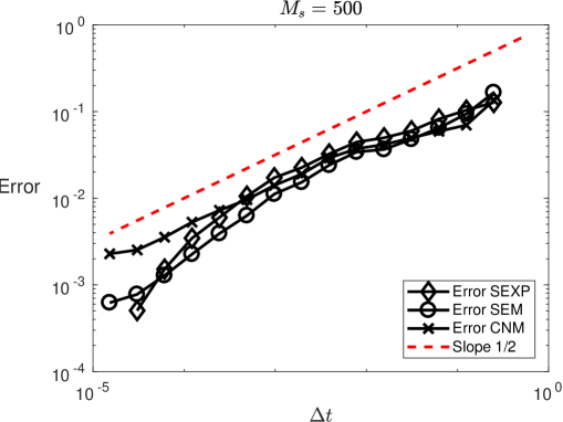
Figure 1: Temporal rates of convergence for the exponential integrator (SEXP), the semi-implicit Euler-Maruyama scheme (SEM), and the Crank-Nicolson-Maruyama scheme (CNM). The reference line has slope $1/2$ (dashed line).

Next, we compare the computational costs of the explicit stochastic exponential method (15), the semi-implicit Euler-Maruyama scheme, and the Crank-Nicolson-Maruyama scheme for the numerical integration of problem (1) with the same parameters as in the previous numerical experiments. We run the numerical methods over the time interval $[0,1]$. We discretize the spatial domain $[0,1]$ with a mesh $\Delta x=2^{-6}$. We run $100$ samples for each numerical method. For each method and each sample, we run several time steps and compare the error at final time with a reference solution provided for the same sample with the same method for the very small time step $\Delta t_{\text{ref}}=2^{-15}$. Figure 2 shows the total computational time for all the samples, for each method and each time step, as a function of the averaged final error we obtain.

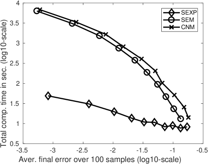
Figure 2: Computational time as a function of the averaged final error for the following numerical methods: the stochastic exponential scheme (15) (SEXP), the semi-implicit Euler-Maruyama (SEM), and the Crank-Nicholson-Maruyama scheme (CNM).

We observe that the computational cost of the Crank-Nicolson-Maruyama scheme is slightly higher than the cost of the semi-implicit Euler-Maruyama scheme which is a little bit higher than the one for the explicit scheme (15).

2.3 Full discretization: almost sure convergence

In this subsection we prove almost sure convergence of the fully discrete approximation $u^{M,N}$ (22) to the exact solution $u$ of the stochastic heat equation (1) with globally Lipschitz continuous coefficients. The main result is the following.

Theorem 2.4.

Assume that the functions $f$ and $\sigma$ satisfy the conditions (LG) and (L), and that $u_{0}\in C([0,1])$ with $u_{0}(0)=u_{0}(1)=0$. Then, the full approximation $u^{M,N}(t,x)$ converges to $u(t,x)$ almost surely, as $M,N\rightarrow\infty$, uniformly in $t\in[0,T]$ and $x\in[0,1]$.

Proof.

In [20, Thm. 3.1], it was shown that $u^{M}(t,x)$ converges to $u(t,x)$ almost surely uniformly in $(t,x)$ as $M\rightarrow\infty$. It is therefore enough to show that $u^{M,N}(t,x)$ converges to $u^{M}(t,x)$ almost surely, as $N\rightarrow\infty$, uniformly in $(t,x)$ and $M\in\mathbb{N}$. To achieve this, it suffices to prove that $w^{M,N}(t,x)$ converges to $w^{M}(t,x)$ almost surely in $(t,x)$ as $N\rightarrow\infty$. This is because the terms involving $u_{0}$ in the approximations $u^{M}$ given by (8) and $u^{M,N}$ given by (22) are the same. We first observe that

$$|w^{M,N}(t,x)-w^{M}(t,x)|^{2p}\leq C(A_{1}+A_{2}+A_{3}),$$

where

$$A_{1} =\sum_{n=0}^{N}\sum_{i=0}^{N}\left|w^{M,N}(t_{n},x_{i})-w^{M}(t_{n},x_{i})\right|^{2p}$$

$$A_{2} =\sup_{n=0,\ldots,N}\sup_{i=0,\ldots,N}\sup_{|x-x_{i}|\leq 1/N}\sup_{|t-t_{n}|\leq\Delta t}\left|w^{M,N}(t,x)-w^{M,N}(t_{n},x_{i})\right|^{2p}$$

$$A_{3} =\sup_{n=0,\ldots,N}\sup_{i=0,\ldots,N}\sup_{|x-x_{i}|\leq 1/N}\sup_{|t-t_{n}|\leq\Delta t}\left|w^{M}(t,x)-w^{M}(t_{n},x_{i})\right|^{2p}$$

and we recall that $x_{i}$ and $t_{n}$ are the discrete points in space and time, respectively, given by $x_{i}=\frac{i}{N}$ for $i=0,1\ldots,N$ and $t_{n}=n\Delta t$ for $n=0,1,\ldots,N$. By Theorem 2.2 we obtain

$$\mathbb{E}[A_{1}]\leq C\left(\frac{1}{N}\right)^{2\mu p-2},$$

for all $0<\mu<\frac{1}{4}$. Also, by Proposition 2.4 we have

$$\mathbb{E}[A_{2}+A_{3}]\leq C\left(\frac{1}{N}\right)^{2p\delta}$$

for $\delta\in(0,1/4)$. Using that

$$\left(\frac{1}{N}\right)^{2\mu p-2}+\left(\frac{1}{N}\right)^{2p\delta}\leq 2\left(\frac{1}{N}\right)^{2p\min(\delta,\mu)-2}$$

we thus get

$$\mathbb{E}\left[\sup_{M\geq 1}\sup_{(t,x)\in[0,T]\times[0,1]}|w^{M,N}(t,x)-w^{M}(t,x)|^{2p}\right]\leq C\left(\frac{1}{N}\right)^{2p\min(\delta,\mu)-2},$$

where the constant $C$ does not depend on $M$ neither on $N$. Hence, using Markov’s inequality we obtain that

$$\mathbb{P}\left(\sup_{M\geq 1}\sup_{(t,x)\in[0,T]\times[0,1]}|w^{M,N}(t,x)-w^{M}(t,x)|^{2p}>\left(\frac{1}{N}\right)^{2}\right)\leq C\left(\frac{1}{N}\right)^{2p\min(\delta,\mu)-4}$$

for all integers $N\geq 1$. It thus follows that

$$\sum_{N=1}^{\infty}\mathbb{P}\left(\sup_{M\geq 1}\sup_{(t,x)\in[0,T]\times[0,1]}|w^{M,N}(t,x)-w^{M}(t,x)|^{2p}>\left(\frac{1}{N}\right)^{2}\right)<\infty$$

for $p$ large enough. By the Borel-Cantelli lemma we now know that for sufficiently large $p$ we have

$$\sup_{M\geq 1}\sup_{(t,x)\in[0,T]\times[0,1]}|w^{M,N}(t,x)-w^{M}(t,x)|^{2p}\leq\frac{1}{N^{2}},$$

with probability one. Taking the limit $N\to\infty$ concludes the proof. ∎

2.3.1 Numerical experiments: almost sure convergence

We now numerically illustrate Theorem 2.4. To do so, we first discretize the stochastic heat equation (1), with $u_{0}(x)=\cos(\pi(x-1/2))$, $f(u)=1-u$, $\sigma(u)=\sin(u)$ with centered finite differences using the mesh $\Delta x=2^{-9}$. The time discretization is done using the explicit exponential integrator (15) with step sizes $\Delta t$ ranging from $2^{-6}$ to $2^{-18}$ (only every second power). Figure 3 displays, for a fixed spatial discretization, profiles of one realization of the numerical solution at the fixed time $T=0.5$ as well as a reference solution computed with the exponential integrator using $\Delta x_{\text{ref}}=2^{-9}$ and $\Delta t_{\text{ref}}=2^{-18}$. Convergence to this reference solution as the time step goes to zero (from light to dark grey plots) is observed.

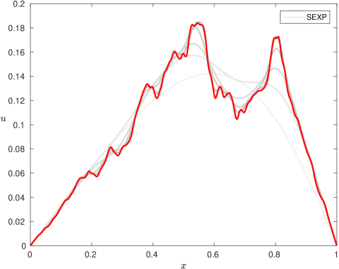
Figure 3: Almost sure convergence of the exponential integrator (SEXP). The reference solution is displayed in red.

3 Convergence analysis for non-globally Lipschitz continuous coefficients

In this section, we remove the globally Lipschitz assumption on the coefficients $f$ and $\sigma$ in equation (1) and we prove convergence in probability of the fully discrete approximation $u^{M,N}$ given by (22) to the exact solution $u$ of (1). Throughout the section we will assume that the initial condition $u_{0}$ belongs to $H^{\beta}$ for some $\beta>\frac{1}{2}$.

Furthermore, we shall consider the following hypotheses:

• Pathwise uniqueness holds for problem (1): whenever $u$ and $v$ are carried by the same filtered probability space and if both $u$ and $v$ are solutions to problem (1) on the stochastic time interval $[0,\tau)$, then $u(t,\cdot)=v(t,\cdot)$ for all $t\in[0,\tau)$, almost surely.

• The coefficient functions $f(t,x,u)$ and $\sigma(t,x,u)$ are continuous in the variable $u$.

Remark 3.1.

For general conditions ensuring pathwise uniqueness in equation (1), we refer the reader to [24, 25]. Nevertheless, note that pathwise uniqueness for parabolic stochastic partial differential equations is an active research topic. Indeed, we mention, for instance, the works [19] (Lipschitz coefficients), [42, 41] (Hölder coefficients), [13, 14] (additive noise), where this question is investigated. These results provide examples of parabolic stochastic partial differential equations where assumption (PU) is fulfilled.

In order to prove the main result of the section (cf Theorem 3.1), we will follow a similar approach as in [20] (see also [44]). More precisely, we will first use the results from Section 2 to deduce that the family of laws determined by $u^{M,N}$ are tight in the space of continuous functions. Then, we will apply Skorokhod’s representation theorem and make use of the weak form (18) corresponding to the fully discrete approximation $u^{M,N}$. Finally, a suitable passage to the limit and assumption (PU) will let us conclude the proof.

We will use the above strategy in a successful way thanks the following two auxiliary results.

Lemma 3.1 (Lemma $4.5$ in [20]).

For all $k\geq 0$, let $z^{k}=\{z^{k}(t,x)\colon t\geq 0,x\in[0,1]\}$ be a continuous $\mathcal{F}_{t}^{k}$-adapted random field and let $W^{k}=\{W^{k}(t,x)\colon t\geq 0,x\in[0,1]\}$ be a Brownian sheet carried by some filtered probability space $(\Omega,\mathcal{F},(\mathcal{F}_{t}^{k})_{t\geq 0},P)$. Assume also that, for every $\epsilon>0$

$$\lim_{k\rightarrow\infty}P\left(\sup_{t\in[0,T]}\sup_{x\in[0,1]}(|z^{k}-z^{0}|+|W^{k}-W^{0}|)(t,x)\geq\epsilon\right)=0.$$

Let $h=h(t,x,r)$ be a bounded Borel function of $(t,x,r)\in\mathbb{R}_{+}\times[0,1]\times\mathbb{R}$, which is continuous in $r\in\mathbb{R}$. Then, letting $k\rightarrow\infty$,

$$\int_{0}^{t}\int_{0}^{1}h(s,x,z^{k}(s,x))\,\mathrm{d}x\,\mathrm{d}s\longrightarrow\int_{0}^{t}\int_{0}^{1}h(s,x,z^{0}(s,x))\,\mathrm{d}x\,\mathrm{d}s,$$

$$\int_{0}^{t}\int_{0}^{1}h(s,x,z^{k}(s,x))\,W^{k}(\mathrm{d}s,\mathrm{d}x)\longrightarrow\int_{0}^{t}\int_{0}^{1}h(s,x,z^{0}(s,x))\,W^{0}(\mathrm{d}s,\mathrm{d}x),$$

in probability for every $t\in[0,T]$.

Lemma 3.2 (Lemma $4.4$ in [20]).

Let $E$ be a Polish space equipped with the Borel $\sigma$-algebra. A sequence of $E$-valued random elements $(z_{n})_{n\geq 1}$ converges in probability if and only if, for every pair of subsequences $z_{l}:=z_{n_{l}}$ and $z_{m}:=z_{n_{m}}$, there exists a subsequence $v_{k}:=(z_{l_{k}},z_{m_{k}})$ converging weakly to a random element $v$ supported on the diagonal $\{(x,y)\in E\times E\colon x=y\}$.

We are now ready to state and prove the main result of this section.

Theorem 3.1.

Assume that the coefficients $f$ and $\sigma$ satisfy condition (LG), and that hypotheses (PU) and (C) are fulfilled. Then, there exists a random field $u=\{u(t,x)\colon t\geq 0,x\in[0,1]\}$ such that, for every $\epsilon>0$,

$$\mathbb{P}\left(\sup_{t\in[0,T]}\sup_{x\in[0,1]}|u^{M_{k},N_{k}}(t,x)-u(t,x)|\geq\epsilon\right)\rightarrow 0,$$

as $k$ tends to infinity, for all sequences of positive integers $(M_{k},N_{k})_{k\geq 1}$ such that $M_{k},N_{k}\rightarrow\infty$, as $k\rightarrow\infty$, where we recall that $u^{M,N}$ denotes the fully discrete solution (22). Furthermore, the random field $u$ is the unique solution to the stochastic heat equation (1).

Proof.

We first show that the sequence $(u^{M,N})_{M,N\geq 1}$ defines a tight family of laws in the space $C([0,T]\times[0,1])$. To do so, we invoke part 2 in Proposition 2.5 on the regularity of the numerical solution and we apply the tightness criterion on the plane [4, Thm. 2.2], which generalizes a well-known result of Billingsley. Furthermore, Prokhorov’s theorem implies that the sequence of laws $(u^{M,N})_{M,N\geq 1}$ is relatively compact in $C([0,T]\times[0,1])$.

Fix any pair of sequences $(M_{k},N_{k})_{k\geq 1}$ such that $M_{k},N_{k}\rightarrow\infty$, as $k\rightarrow\infty$. Then, the laws of $v_{k}:=u^{M_{k},N_{k}}$, $k\geq 1$, form a tight family in the space $C([0,T]\times[0,1])$.

Let now $(v^{1}_{j})_{j\geq 1}$ and $(v^{2}_{\ell})_{\ell\geq 1}$ be two subsequences of $(v_{k})_{k\geq 1}$. By Skorokhod’s Representation Theorem, there exist subsequences of positive integers $(j_{r})_{r\geq 1}$ and $(\ell_{r})_{r\geq 1}$ of the indices $j$ and $\ell$, a probability space $(\widehat{\Omega},\widehat{\mathcal{F}},(\widehat{\mathcal{F}_{t}})_{t\geq 1},\widehat{\mathbb{P}})$, and a sequence of continuous random fields $(z_{r})_{r\geq 1}$ with $z_{r}:=\bigl{(}\widetilde{u}_{r},\overline{u}_{r},\widehat{W}_{r}\bigr{)}$, $r\geq 1$, such that

1. $z_{r}\underset{r\to\infty}{\longrightarrow}z:=(\widetilde{u},\overline{u},\widehat{W})$ a.s. in $C([0,T]\times[0,1],\mathbb{R}^{3})$, where the random field $z$ is defined on $(\widehat{\Omega},\widehat{\mathcal{F}},(\widehat{\mathcal{F}_{t}})_{t\geq 1},\widehat{\mathbb{P}})$, $\widehat{W}$ is a Brownian sheet defined on this basis, and $\widehat{\mathcal{F}_{t}}=\sigma(z(s,x),\,(s,x)\in[0,t]\times[0,1])$ (and conveniently completed).

2. For every $r\geq 1$, the finite dimensional distributions of $z_{r}$ coincide with those of the random field $\zeta_{r}:=\bigl{(}v^{1}_{j_{r}},v^{2}_{\ell_{r}},W\bigr{)}$, and thus $\text{law}(z_{r})=\text{law}(\zeta_{r})$ for all $r\geq 1$.

Note that $\widehat{W}_{r}$ is a Brownian sheet defined on $(\widehat{\Omega},\widehat{\mathcal{F}},(\widehat{\mathcal{F}^{r}_{t}})_{t\geq 1},\widehat{\mathbb{P}})$, where $\widehat{\mathcal{F}^{r}_{t}}=\sigma(z_{r}(s,x),\\ (s,x)\in[0,t]\times[0,1])$ (and conveniently completed).

We now fix $(t,x)\in[0,T]\times[0,1]$. Since the laws of $z_{r}$ and $\zeta_{r}$ coincide and the first two components of $\zeta_{r}$ satisfy the weak form (18), so do the components of $z_{r}$. Namely, for all $\Phi\in C^{\infty}(\mathbb{R}^{2})$ with $\Phi(t,0)=\Phi(t,1)=0$ for all $t$, it holds

$$\int_{0}^{1}\widetilde{u}_{r}(t,\kappa_{M}(y))\Phi(t,y)\,\mathrm{d}y= \int_{0}^{1}u_{0}(\kappa_{M}(y))\Phi(t,y)\,\mathrm{d}y$$

$$\quad+\int_{0}^{t}\int_{0}^{1}\widetilde{u}_{r}(s,\kappa_{M}(y))\left(\Delta_{M}\Phi(s,y)+\frac{\partial\Phi}{\partial s}(s,y)\right)\,\mathrm{d}y\,\mathrm{d}s$$

$$\quad+\int_{0}^{t}\int_{0}^{1}f(\widetilde{u}_{r}(\kappa_{N}^{T}(s),\kappa_{M}(y)))\Phi(s,y)\,\mathrm{d}y\,\mathrm{d}s$$

$$\quad+\int_{0}^{t}\int_{0}^{1}\sigma(\widetilde{u}_{r}(\kappa_{N}^{T}(s),\kappa_{M}(y)))\Phi(s,y)\,W(\mathrm{d}s,\mathrm{d}y),\quad\widehat{\mathbb{P}}\text{-a.s.},$$ (26)

for all $t\in[0,T]$, and also

$$\int_{0}^{1}\overline{u}_{r}(t,\kappa_{M}(y))\Phi(t,y)\,\mathrm{d}y= \int_{0}^{1}u_{0}(\kappa_{M}(y))\Phi(t,y)\,\mathrm{d}y$$

$$\quad+\int_{0}^{t}\int_{0}^{1}\overline{u}_{r}(s,\kappa_{M}(y))\left(\Delta_{M}\Phi(s,y)+\frac{\partial\Phi}{\partial s}(s,y)\right)\,\mathrm{d}y\,\mathrm{d}s$$

$$\quad+\int_{0}^{t}\int_{0}^{1}f(\overline{u}_{r}(\kappa_{N}^{T}(s),\kappa_{M}(y)))\Phi(s,y)\,\mathrm{d}y\,\mathrm{d}s$$

$$\quad+\int_{0}^{t}\int_{0}^{1}\sigma(\overline{u}_{r}(\kappa_{N}^{T}(s),\kappa_{M}(y)))\Phi(s,y)\,W(\mathrm{d}s,\mathrm{d}y),\quad\widehat{\mathbb{P}}\text{-a.s.},$$ (27)

for all $t\in[0,T]$. We recall that $\Delta_{M}$ denotes the discrete Laplacian, which is defined by

$$\Delta_{M}\Phi(s,y):=(\Delta x)^{-2}\left\{\Phi(s,y+\Delta x)-2\Phi(s,y)+\Phi(s,y-\Delta x)\right\},$$

where we remind that $\Delta x=\frac{1}{M}$.

Taking $r\rightarrow\infty$ in the above formulas (26) and (27), and using Lemma 3.1, we show that the random fields $\tilde{u}$ and $\bar{u}$ are solutions of (2), and hence of equation (1), on the same stochastic basis $(\widehat{\Omega},\widehat{\mathcal{F}},(\widehat{\mathcal{F}_{t}})_{t\geq 1},\widehat{\mathbb{P}})$. Thus, by the pathwise uniqueness assumption, we obtain that $\widetilde{u}(t,x)=\overline{u}(t,x)$ for all $(t,x)\in[0,T]\times[0,1]\>\>$ $\widehat{\mathbb{P}}$-a.s. Hence, by Lemma 3.2, we get that $\{u^{M_{k},N_{k}}\}_{k\geq 1}$ converges in probability to $u$, uniformly on $[0,T]\times[0,1]$, the solution of the stochastic heat equation (1). ∎

4 Acknowledgement

L. Quer-Sardanyons’ research is supported by grants 2014SGR422 and MTM2015-67802-P. This work was partially supported by the Swedish Research Council (VR) (project nr. $2013-4562$). The computations were performed on resources provided by the Swedish National Infrastructure for Computing (SNIC) at HPC2N, Umeå University.

References

[1]
E. J. Allen, S. J. Novosel, and Z. Zhang.
Finite element and difference approximation of some linear stochastic
partial differential equations.
Stochastics Stochastics Rep., 64(1-2):117–142, 1998.
[2]
R. Anton and D. Cohen.
Exponential integrators for stochastic Schrödinger equations
driven by Itô noise.
To appear in the special issue on SPDEs of J. Comput. Math,
2017.
[3]
R. Anton, D. Cohen, S. Larsson, and X. Wang.
Full discretization of semilinear stochastic wave equations driven by
multiplicative noise.
SIAM J. Numer. Anal., 54(2):1093–1119, 2016.
[4]
X. Bardina, M. Jolis, and L. Quer-Sardanyons.
Weak convergence for the stochastic heat equation driven by
Gaussian white noise.
Electron. J. Probab., 15:no. 39, 1267–1295, 2010.
[5]
A. Barth and A. Lang.
Simulation of stochastic partial differential equations using finite
element methods.
Stochastics, 84(2-3):217–231, 2012.
[6]
A. Barth and A. Lang.
and almost sure convergence of a Milstein scheme for
stochastic partial differential equations.
Stochastic Process. Appl., 123(5):1563–1587, 2013.
[7]
S. Becker, A. Jentzen, and P. E. Kloeden.
An exponential Wagner-Platen type scheme for SPDEs.
SIAM J. Numer. Anal., 54(4):2389–2426, 2016.
[8]
D. Cohen and G. Dujardin.
Exponential integrators for nonlinear schrödinger equations with
white noise dispersion.
Stochastics and Partial Differential Equations: Analysis and
Computations, pages 1–22, 2017.
[9]
D. Cohen, S. Larsson, and M. Sigg.
A trigonometric method for the linear stochastic wave equation.
SIAM J. Numer. Anal., 51(1):204–222, 2013.
[10]
D. Cohen and L. Quer-Sardanyons.