Accelerated cosmos in a non-extensive setup

Abstract

Here, we consider a flat FRW universe whose its horizon entropy meets the Rényi entropy of non-extensive systems. In our model, the ordinary energy-momentum conservation law is not always valid. By applying the Clausius relation as well as the Cai-Kim temperature to the apparent horizon of a flat FRW universe, we obtain modified Friedmann equations. Fitting the model to the observational data on current accelerated universe, some values for the model parameters are also addressed. Our study shows that the current accelerating phase of universe expansion may be described by a geometrical fluid, originated from the non-extensive aspects of geometry, which models a varying dark energy source interacting with matter field in the Rastall way. Moreover, our results indicate that the probable non-extensive features of spacetime may also be used to model a varying dark energy source which does not interact with matter field, and is compatible with the current accelerated phase of universe.

I Introduction

The violation of energy-momentum conservation law in curved spacetime has firstly been proposed by P. Rastall to modify general relativity theory of Einstein (GR) rastall . After his pioneering work, various type of modified gravity in which matter fields are non-minimally coupled to geometry have been proposed cmc ; cmc1 ; cmc2 ; genras ; PRL ; shabprl ; shabprl1 . It has been shown the Rastall correction term to the Einstein field equations can not describe dark energy meaning that a dark energy-like source is needed to model the current phase of universe expansion in this framework prd . But, if one generalizes this theory in a suitable manner, then the mutual non-minimal coupling between geometry and matter field may be considered as the origin of the current accelerating phase and the inflation era genras . More studies on Rastall theory can be found in Refs. gc1 ; al1 ; al2 ; al3 ; smal ; Rlag ; obs1 ; rastbr ; rascos1 ; rasch ; more1 ; more2 ; more3 ; more4 ; more5 ; hm ; msal ; plb1c ; msh ; clm ; net .

In Einstein gravity, horizons may meet the Bekenstein-Hawking entropy-area law which is a non-extensive entropy rn1 ; rn2 ; rn4 ; rn5 ; rn6 ; rn7 ; rn8 ; rn9 ; rn10 ; rn11 ; rn12 ; rn13 ; rn14 ; rn15 ; rn16 ; rey2 . Moreover, it has recently been argued that a deep connection between dark energy and horizon entropy may exist in gravitational theories cana ; cana1 ; mmg ; em ; mitra ; mitra1 ; mitra2 ; mitra3 ; mms ; md ; msgj ; mswr . Indeed, although extensive statistical mechanics and its corresponding thermodynamics lead to interesting results about the universe expansion history mrej , the mentioned points encourage physicists to use non-extensive statistical mechanics reyo1 ; tsallis in order to study the thermodynamic properties of spacetime and its related subjects rn3 ; rey1 ; rsal1 ; rsal2 ; rsal ; anp ; ijtp ; cite5 ; Kom1 ; Kom2 ; Kom3 ; Kom ; EPJC ; MSK .

Recently, applying Rényi entropy to the horizon of FRW universe and considering a varying dark energy source interacting with matter field, N. Komatsu found out modified Friedmann equations in agreement with observational data on the current phase of universe expansion EPJC . Therefore, in his model, total energy-momentum tensor including the matter field and varying dark energy-like source is conserved. Combining this entropy with entropic force scenario, one can also obtain a theoretical basis for the MOND theory MSK . In fact, the probable non-extensive features of spacetime may be considered as an origin for both the MOND theory and the current accelerated expansion phase in a universe filled by a pressureless source satisfying ordinary conservation law MSK . Finally, it is useful to note here that both mentioned attempts EPJC ; MSK used the Padmanabhan holographic approach Padd in getting their models of the universe expansion.

Here, we are interested in obtaining a model for the universe dynamics by applying the Clausius relation as well as the Rényi entropy to the horizon of FRW universe which has non-minimally been coupled to matter field. Therefore, total energy-momentum tensor does not necessarily satisfy the ordinary conservation law, and in fact, it follows the Rastall hypothesis in our setup.

The paper is organized as follows. In the next section, introducing our approach, we present a thermodynamic description for Friedmann equations in Rastall theory. Using the Rényi entropy, our model of universe is obtained in Sec. (III). In the fourth section, we consider a universe filled by a pressureless source, and show that, in our formalism, it can experience an accelerated expansion. Sec. (V) includes the observational constraints of model. The last section is devoted to a summary and concluding remarks. We use the unit of $c=\hbar=k_{B}=1$ in our calculations.

II Thermodynamic description of Friedmann equations in Rastall theory

Based on the Rastall hypothesis rastall

$$T^{\mu}_{\ \nu\ ;\mu}=\lambda R_{,\nu},$$ (1)

where $\lambda$ denotes the Rastall constant parameter, and $T^{\mu\nu}$ is the energy-momentum tensor of source which fills background. Moreover, $R$ is the Ricci scalar of spacetime. This equation says that there is an energy exchange between spacetime and cosmic fluids due to the tendency of geometry to couple with matter fields in a non-minimal way genras ; clm . For example, the $\lambda=\frac{1}{4k}$ case, where $k$ is called the Rastall gravitational coupling constant, can support the primary inflationary era in an empty FRW universe genras . In this manner, the ability of geometry to couple with matter fields in a non-minimal way generates a constant energy density equal to $\lambda R$ genras . Some features of this non-minimal mutual interaction and its corresponding energy flux as well as its applications in cosmic eras have been studied in Ref. genras .

Bearing the Bianchi identity in mind and integrating Eq. (1), one can reach at rastall

$$G_{\mu\nu}+k\lambda g_{\mu\nu}R=kT_{\mu\nu}.$$ (2)

The Newtonian limit of the Rastall theory implies msal ; msh

$$k=\frac{\gamma}{\lambda}=\frac{4\gamma-1}{6\gamma-1}8\pi G,$$ (3)

where $\gamma\equiv k\lambda$. Applying the thermodynamic laws to the horizon of spacetime and using Eqs. (2) and (3), it is shown that the horizon entropy is achieved as hm ; msal ; plb1c

$$S_{A}^{R}=\frac{2\pi A}{k},$$ (4)

in which $A$ is the horizon area. Combining this result with Eq. (3), one can easily find that entropy is positive whenever $\gamma$ either meets the $\gamma<\frac{1}{6}$ or $\gamma>\frac{1}{4}$ condition msal . This equation can also be written as $S_{A}^{R}=\frac{6\gamma-1}{4\gamma-1}S_{B}$, where $S_{B}=\frac{A}{4G}$ is the Bekenstein-Hawking entropy msal , meaning that the second law of thermodynamics is obtained for the mentioned values of $\gamma$, if it is satisfied by the Bekenstein-Hawking entropy. In addition, simple calculation lead to

$$\lambda=\frac{\gamma}{k}=\frac{\gamma(6\gamma-1)}{(4\gamma-1)8\pi G},$$ (5)

for the Rastall constant parameter msal . Indeed, Eqs. (3) and (5) are the direct results of imposing the Newtonian limit on Eq. (2), indicating that only for $\lambda=\gamma=0$ we have $k=8\pi G$ rastall ; msh . In Ref. net , assuming $k=8\pi G$ and studying Neutron stars in Rastall gravity, authors found out that $\lambda$ is so close to zero. Therefore, we see that since they consider $k=8\pi G$, their result does not reject the Rastall hypothesis. Finally, it is worth to remind here that the Bekenstein-Hawking entropy ($S_{B}=\frac{A}{4G}$) is also obtainable at the appropriate limit of $\gamma\rightarrow 0$.

For a flat FRW universe with scale factor $a(t)$ and line element

$$ds^{2}=-dt^{2}+a(t)^{2}[dr^{2}+r^{2}(d\theta^{2}+\sin(\theta)^{2}d\phi^{2})],$$ (6)

the apparent horizon, equal to the Hubble horizon, is located at

$$\tilde{r}_{A}=a(t)r_{A}=\frac{1}{H},$$ (7)

and therefore $A=\frac{4\pi}{H^{2}}$. Now, if the geometry is filled by a prefect fluid with energy density $\rho$ and pressure $p$ ($T^{\mu}_{\ \nu}=diag(-\rho,p,p,p)$), then Eq. (1) leads to

$$\dot{\rho}+3H(\rho+p)=-\lambda\dot{R},$$ (8)

where dot denotes derivative with respect to time. It is also useful to remind here that for the flat FRW universe

$$R=6\big{[}(\frac{\dot{a}}{a})^{2}+\frac{\ddot{a}}{a}\big{]}.$$ (9)

Moreover, the use of Eq. (2) yields hm

$$(12\gamma-3)H^{2}+6\gamma\dot{H}=-\frac{4\gamma-1}{6\gamma-1}8\pi G\rho,$$ (10)

$$(12\gamma-3)H^{2}+(6\gamma-2)\dot{H}=\frac{4\gamma-1}{6\gamma-1}8\pi Gp,$$

The evolution of density perturbation in this model has been studied in Refs. prd ; rascos1 ; obs1 . It has been shown that the story is the same as those of the standard cosmology at the background and linear perturbation level prd . Finally, one can use Eqs. (10) to get hm

$$\dot{H}=-\frac{k}{2}(\rho+p).$$ (11)

From the standpoint of tensor calculus, Eq. (2) is a solution for Eq. (1) leading to the above results. But, does thermodynamics lead to the same solutions? Indeed, since entropy is the backbone of thermodynamic approach, it is expected that Eq. (2) and thus the above results are available only whenever the horizon entropy meets Eq. (4). In order to find the Friedmann equations corresponding on Eq. (1) from the thermodynamics point of view, we consider the general form of entropy as $S_{A}=S(\frac{2\pi A}{k})$. Additionally, one can use

$$\delta Q^{m}=(T^{b}_{a}\partial_{b}\tilde{r}+W\partial_{a}\tilde{r})dx^{a},$$ (12)

to evaluate the energy flux crossing the apparent horizon Cai2 ; CaiKim . Here, we also focus on an energy-momentum source as $T_{\mu}^{\nu}=\textmd{diag}(-\rho,p,p,p)$ which yields $W=\frac{\rho-p}{2}$ for the work density. Finally, we see hm ; plb1c

$$\delta Q^{m}=-A(\rho+p)dt.$$ (13)

Now, applying the Clausius relation ($TdS_{A}=-\delta Q^{m}$) to horizon abe , and using the Cai-Kim temperature ($T=\frac{H}{2\pi}$) CaiKimt , one can easily find

$$\dot{H}=-\frac{\pi}{S^{\prime}}(\rho+p),$$ (14)

where $S^{\prime}=\frac{dS_{A}}{dA}$ pwang . Now, combining this result with Eq. (8), we obtain

$$S^{\prime}dH^{2}=\frac{2\pi}{3}d(\rho+\lambda R),$$ (15)

as the differential form of the first Friedmann equation. The result of this equation can be combined with Eq. (14) to get the second Friedmann equation.

Now, if the system entropy meets Eq. (4), then Eq. (14) leads to $2\dot{H}=-k(\rho+p)$. It is also easy to insert Eq. (4) into Eq. (15) to get

$$(12\gamma-3)H^{2}+6\gamma\dot{H}+\mathcal{C}=-\frac{4\gamma-1}{6\gamma-1}8\pi G\rho,$$ (16)

where, $\mathcal{C}$ is the integration constant of Eq. (15). Now, adding and subtracting $2\dot{H}$ from the LHS this equation, and using the $2\dot{H}=-k(\rho+p)$ relation, we can reach at

$$(12\gamma-3)H^{2}+(6\gamma-2)\dot{H}+\mathcal{C}=\frac{4\gamma-1}{6\gamma-1}8\pi Gp.$$ (17)

It is apparent that, for the $\mathcal{C}=0$ case, the original Friedmann equations in the Rastall framework are reproduced (16). Indeed, since divergence of $\mathcal{C}g_{\mu\nu}$ is zero, one may add the $\mathcal{C}g_{\mu\nu}$ term to the RHS of Rastall field equations (2) to directly get Eq. (16) instead of Eq. (10). Anyway, we know that this term represents an unusual fluid in the context of ordinary physics leading to dark energy concept and thus its problems.

Now, Let us consider a flat FRW universe filled by a fluid with constant state parameter defined as $w=\frac{p}{\rho}$. In this manner, calculations lead to hm

$$\rho=\rho_{0}a^{\frac{-3(1+\omega)(4\gamma-1)}{3\gamma(1+\omega)-1}},$$ (18)

where $\rho_{0}$ is constant, for the energy density profile. For a universe filled by a pressureless component, where $\rho=\rho_{0}a^{\frac{-3(4\gamma-1)}{3\gamma-1}}$, combining this equation with Eqs. (16), one reaches at

$$\dot{H}=-\frac{\rho_{0}(4\gamma-1)4\pi G}{6\gamma-1}a^{\frac{-3(4\gamma-1)}{3\gamma-1}},$$ (19)

and

$$H^{2}=\frac{\rho_{0}(3\gamma-1)8\pi G}{3(6\gamma-1)}a^{\frac{-3(4\gamma-1)}{3\gamma-1}}+\mathcal{C}.$$ (20)

Now, it is natural expectation that the matter density should be diluted during the expansion of universe. This limits us to the Rastall theories with $\gamma<\frac{1}{4}$ and $\frac{1}{3}<\gamma$. Applying this result to Eq. (19), we find out that, at the long run limit ($a(t)\gg 1$), we have $\dot{H}\rightarrow 0$, and therefore, universe may experience an accelerating phase. In this situation, Eq. (20) implies $H=H_{0}\approx\mathcal{C}$ meaning that a non-minimal coupling between geometry and energy-momentum source cannot describe the current accelerating phase of universe in the Rastall framework. In fact, as it is apparent, we should have $\mathcal{C}\neq 0$ to get $H_{0}\neq 0$, and thus, an accelerating universe. Therefore, the same as the standard Friedmann equations, a dark energy-like source is needed to model the accelerating universe in the Rastall theory, a result in agreement with recent study by Batista et al. prd .

In summary, our thermodynamic based study shows the dark energy problem is also valid in this formalism prd , unless one generalizes the Rastall theory in a suitable manner genras .

III Rényi entropy and Friedmann equations

Recently, Rényi entropy has been used in order to study the effects of probable non-extensive aspects of spacetime which led to interesting results in both cosmological and gravitational setups rey1 ; rey2 ; EPJC ; MSK ; rey03 ; rey04 ; rey05 ; rey06 . For a non-extensive system including $W$ discrete states, the Rényi entropy is defined as reyo1

$$\mathcal{S}=\frac{1}{1-q}\ln\sum_{i=1}^{W}P_{i}^{q},$$ (21)

in which $P_{i}$ and $q$ denote the probability of $i^{th}$ state and the non-extensive parameter, respectively. Moreover, the Tsallis entropy of this system is as follows tsallis

$$S_{T}=\frac{1}{1-q}\sum_{i=1}^{W}(P_{i}^{q}-P_{i}).$$ (22)

The linear relation between entropy and area is the key point of the Bekenstein-Hawking entropy ($S_{B}\sim A$), which can also be obtained from the Tsallis’ non-additive entropy definition rn3 . As it is apparent from Eq. (4), the functionality of $S_{A}^{R}$ with respect to the horizon area ($A$) is the same as that of the Bekenstein-Hawking entropy ($S_{A}^{R}\sim A$) meaning that $S_{A}^{R}$ may be considered as a special case of Eq. (22). More detailed studies on gravitational and cosmological implications of Tsallis entropy (22) can be found in Refs. rn3 ; rsal1 ; rsal2 ; rsal ; anp ; ijtp ; cite5 ; Kom1 ; Kom2 ; Kom3 and references therein. Eq. (22) can be combined with Eq. (21) to show that

$$\mathcal{S}=\frac{1}{\delta}\ln(1+\delta S_{T}),$$ (23)

where $\delta\equiv 1-q$, and we used $\sum_{i=1}^{W}P_{i}=1$ to obtain this equation rey1 ; MSK . It has frequently been argued that the Bekenstein-Hawking entropy is not an extensive entropy rn1 ; rn2 ; rn4 ; rn5 ; rn6 ; rn7 ; rn8 ; rn9 ; rn10 ; rn11 ; rn12 ; rn13 ; rn14 ; rn15 ; rn16 ; rey2 , and in fact, the Bekenstein-Hawking entropy can be considered as a proper candidate for $S_{T}$ in gravitational and cosmological setups rey1 ; rey2 ; EPJC ; MSK , a choice in full agreement with Ref. rn3 . Here, following the above arguments and recent studies rn3 ; rey1 ; rey2 ; EPJC ; MSK , we use Eq. (4) as the Tsallis entropy candidate in our calculations leading to

$$\mathcal{S}_{A} = \frac{1}{\delta}\ln(1+\delta S_{A}^{R})=\frac{1}{\delta}\ln(1+\frac{2\pi\delta}{k}A),$$ (24)

$$\mathcal{S}_{A}^{\prime} = \frac{d\mathcal{S}_{A}}{dA}=\frac{2\pi H^{2}}{k[H^{2}+\Delta]},$$ (25)

for the Rényi entropy of horizon ($\mathcal{S}_{A}$) and its derivative with respect to $A$ ($\mathcal{S}_{A}^{\prime}$), respectively. Here, $\Delta\equiv\frac{(6\gamma-1)\delta\pi}{(4\gamma-1)G}$, and it is easy to check that whenever the non-extensive features of system approach zero (or equally $\delta\rightarrow 0$), the $\mathcal{S}_{A}$ relation recovers Eq. (4). Now, inserting Eq. (25) into Eqs. (14) and (15), one can obtain

$$\dot{H}=-\frac{k[H^{2}+\Delta]}{2H^{2}}(\rho+p),$$ (26)

and

$$H^{2}-\Delta\ln(\Delta+H^{2})+C_{1}=\frac{k}{3}\rho+\frac{\gamma}{3}R,$$ (27)

where $C_{1}$ is the integration constant, respectively. Defining a new constant $C=C_{1}-\Delta\ln\Delta$, one can rewrite the last equation as

$$H^{2}-\Delta\ln(1+\frac{H^{2}}{\Delta})+C=\frac{k}{3}\rho+\frac{\gamma}{3}R.$$ (28)

Since $H=\frac{\dot{a}}{{a}}$, Eq. (9) can be rewritten as

$$R=6(\dot{H}+2H^{2}).$$ (29)

Finally, combining this equation with Eq. (28), and inserting the result into Eq. (26), we find

$$H^{2}=\frac{k}{3}(\rho+\rho_{e}^{\gamma}),$$ (30)

and

$$H^{2}+\frac{2}{3}\dot{H}=-\frac{k}{3}(p+p_{e}^{\gamma}),$$ (31)

for the first and second Friedmann equations in our model, respectively. In fact, one should combine Eqs. (30) and (26) with each other, and then add and subtract the $\frac{2}{3}\dot{H}$ term to the result to find the last equation. In the above equations,

$$\rho_{e}^{\gamma} = \frac{3}{k}\bigg{(}4\gamma H^{2}+\Delta\ln(1+\frac{H^{2}}{\Delta})+2\gamma\dot{H}-C\bigg{)},$$

$$p_{e}^{\gamma} = -\frac{3}{k}\bigg{(}4\gamma H^{2}+\Delta\ln(1+\frac{H^{2}}{\Delta})$$

$$+ 2\dot{H}(\gamma+\frac{1}{3(\frac{H^{2}}{\Delta}+1)})-C\bigg{)},$$

denote effective energy density and effective pressure in this framework, respectively. It is easy to see that, at the $\delta\rightarrow 0$ limit (or equally $\Delta\rightarrow 0$), the results of Rastall theory are recovered. Additionally, we have $p_{e}\rightarrow-\rho_{e}$ whenever $\dot{H}\rightarrow 0$. Now, since $\frac{\ddot{a}}{a}=H^{2}+\dot{H}$, one can rewrite Eq. (31) as

$$2\frac{\ddot{a}}{a}+H^{2}=-k(p+p_{e}^{\gamma}),$$ (33)

where its LHS has the same form as that of the standard Friedmann equation roos . Besides, simple calculations reach

$$\frac{\ddot{a}}{a}=-\frac{k}{6}[\rho+\rho_{e}^{\gamma}+3(p+p_{e}^{\gamma})],$$ (34)

for the acceleration equation. Therefore, we deal with two fluids. The first fluid is the ordinary energy-momentum tensor $T_{\mu}^{\nu}$ corresponding to the real fluid with energy density $\rho$ and pressure $p$. The second fluid, which has geometrical origin, is called the effective energy-momentum tensor, and it is defined as

$$\Theta_{\mu}^{\nu}=diag(-\rho_{e}^{\gamma},p_{e}^{\gamma},p_{e}^{\gamma},p_{e}^{\gamma}).$$ (35)

In fact, the obtained effective fluid consists of two parts: $i)$ the non-extensive aspects of spacetime, and $ii)$ the non-minimal coupling between geometry and matter fields which follows the Rastall hypothesis. Therefore, the $\gamma\rightarrow 0$ limit of $\Theta_{\mu}^{\nu}$ only includes the non-extensive effects. We show it by $\mathcal{T}_{\mu}^{\nu}=diag(-\rho_{e},p_{e},p_{e},p_{e})$ in which

$$\rho_{e}=\frac{3}{8\pi G}\bigg{(}\Delta_{(\gamma=0)}\ln(1+\frac{H^{2}}{\Delta_{(\gamma=0)}})-C_{(\gamma=0)}\bigg{)},$$

$$p_{e}=-\rho_{e}-\frac{3}{8\pi G}\bigg{(}\frac{2\dot{H}}{3(\frac{H^{2}}{\Delta_{(\gamma=0)}}+1)}\bigg{)},$$ (36)

where $\Delta_{(\gamma=0)}=\frac{\delta\pi}{G}$ and $C_{(\gamma=0)}=C_{1}-\Delta_{(\gamma=0)}\ln\Delta_{(\gamma=0)}$. In fact, it is a geometrical fluid originated from the non-extensive aspects of spacetime, and recovers the ordinary cosmological constant model of dark energy at the appropriate limit of $\gamma\rightarrow 0$. It is also easy to check that this source satisfies the conservation law i.e.

$$\dot{\rho}_{e}+3H(\rho_{e}+p_{e})=0,$$ (37)

Therefore, $\Theta_{\mu}^{\nu}$ acts as a time-varying dark energy model which satisfies the conservation law only for $\gamma=0$.

Bearing the Bianchi identity in mind, since the LHS of Eqs. (30) and (33) are compatible with the Einstein tensor, we should have $(\Theta_{\mu}^{\nu}+T_{\mu}^{\nu})^{;\mu}=0$ leading to

$$\dot{\rho}+3H(\rho+p)=-[\dot{\rho}_{e}^{\gamma}+3H(\rho_{e}^{\gamma}+p_{e}^{\gamma})],$$ (38)

and thus

$$\lambda\dot{R}=\dot{\rho}_{e}^{\gamma}+3H(\rho_{e}^{\gamma}+p_{e}^{\gamma}).$$ (39)

In fact, the above results would also be obtained by writing Einstein field equations as $G_{\mu\nu}=k(\Theta_{\mu\nu}+T_{\mu\nu})$. In addition, Eqs. (37) and (39) tell us that there is no energy flux between geometry and matter fields at the appropriate limit of $\lambda\rightarrow 0$ (or equally $\gamma\rightarrow 0$), a result in full agreement with Eq. (1). Indeed, although $\Theta_{\mu}^{\nu}\rightarrow\mathcal{T}_{\mu}^{\nu}$ at the $\gamma\rightarrow 0$ limit, since $\mathcal{T}_{\mu}^{\nu}$ is a divergence-less tensor (37), we have $\lambda\dot{R}=0$ and thus the ordinary energy-momentum conservation law is met by the $T_{\mu}^{\nu}$ source. Applying the $\gamma\rightarrow 0$ and $\Delta\rightarrow 0$ limits to the above equations, one can easily reach at the standard Friedmann equations compatible with the Bekenstein-Hawking entropy of horizon ijtp ; md ; em . Therefore, the $\gamma\rightarrow 0$ limit helps us in obtaining the modification of considering Rényi entropy to the standard Friedmann equations as

$$H^{2}=\frac{8\pi G}{3}(\rho+\rho_{e}),$$ (40)

$$H^{2}+\frac{2}{3}\dot{H}=\frac{-8\pi G}{3}(p+p_{e}),$$

where $\rho_{e}$ and $p_{e}$ follow Eq. (III). It is worth to mention that, independent of the values of $C$ and $\Delta$, we have $p_{e}\rightarrow-\rho_{e}$ whenever $\dot{H}\rightarrow 0$. As a check, one can also insert $\gamma=0$ in Eqs. (3) and (III) to get these results. In this manner, the acceleration equation is

$$\frac{\ddot{a}}{a}=-\frac{4\pi G}{3}[\rho+\rho_{e}+3(p+p_{e})],$$ (41)

and the second line of Eq. (40) can also be written as

$$2\frac{\ddot{a}}{a}+H^{2}=-8\pi G(p+p_{e}),$$ (42)

where its LHS is in the form of the standard Friedmann equation roos . Bearing Eq. (37) as well as the argument after Eq. (39) in mind, it is apparent that, for $\gamma=0$, the $T_{\mu\nu}$ source respects the continuity equation i.e.

$$\dot{\rho}+3H(\rho+p)=0.$$ (43)

Although the same as Refs. EPJC ; MSK , we used the Rényi entropy to get the modified Friedmann equations, these equations differ from those of recent studies EPJC ; MSK . It has three reasons. i) While the entropy expression appears in acceleration equations obtained in Refs. EPJC ; MSK , which use the Padmanabhan approach, its derivative is the backbone of getting the acceleration equation in our model based on applying thermodynamics laws to horizon (see Eq. (14)). ii) The Komar mass definition has been used by authors in Refs. EPJC ; MSK only for the $T_{\mu\nu}$ source. As we saw, our results are also obtainable if one writes the Einstein field equations as $G_{\mu\nu}=k(\Theta_{\mu\nu}+T_{\mu\nu})$ meaning that the Komar mass should be written for the modified energy-momentum tensor $\Theta_{\mu\nu}+T_{\mu\nu}$ instead of $T_{\mu\nu}$. iii) In Ref. EPJC , the non-extensive features of spacetime has been introduced as an origin for a time-varying dark energy ($\Lambda(t)$) which interacts with matter fields and does not meet Eq. (37). This is while time-varying dark energy candidate of our model interacts with matter fields only in the Rastall way, and meets Eq. (37) in the absence of the Rastall hypothesis ($\gamma=0$).

IV A Universe filled by a pressureless fluid

In order to study a universe filled by a pressureless source, we insert $\rho=\rho_{0}a^{\frac{-3(4\gamma-1)}{3\gamma-1}}$ into Eq. (26) and use Eq. (30) to reach at

$$\frac{H^{2}(1-4\gamma)-\Delta\ln(1+\frac{H^{2}}{\Delta})+C}{1-3\gamma(1+\frac{\Delta}{H^{2}})}=\xi a^{\frac{-3(4\gamma-1)}{3\gamma-1}},$$ (44)

where $\xi\equiv\frac{\rho_{0}(4\gamma-1)8\pi G}{3(6\gamma-1)}$. It is clear that, for a Rastall theory of $\gamma<\frac{1}{4}$ or $\frac{1}{3}<\gamma$, the RHS of this equation and thus its LHS are vanished at long run limit ($a\gg 1$) meaning that $H\rightarrow constant\equiv H_{0}$. Now, $H_{0}$ can be evaluated from

$$\frac{H_{0}^{2}}{\Delta}=\frac{\ln(1+\frac{H_{0}^{2}}{\Delta})}{1-4\gamma}+C_{2},$$ (45)

where $C_{2}\equiv\frac{C}{(4\gamma-1)\Delta}$ is a constant. It is also apparent that, depending on the value of $\gamma$, this equation may be solvable even if we have $C_{2}=0$ or $C_{1}=0$. Additionally, since $\Delta$ is unknown parameter, this equation helps us in finding its possible values as a function of $H_{0}$. One can also use this result in order to apply the $a\gg 1$ limit to Eq. (26) to see that $\dot{H}\rightarrow 0$ whenever $\gamma$ meets either $\gamma<\frac{1}{4}$ or $\frac{1}{3}<\gamma$. In summary, based on our results, the dark energy problem in Rastall theory can be overcame by considering the probable non-extensive features of spacetime.

Now, we consider a universe filled by a pressureless source ($p=0$) whenever $\gamma=0$. In this manner, both of Eqs. (18) and (43) lead to $\rho=\rho_{0}a^{-3}$ for energy density. Inserting $\gamma=0$ into Eqs. (40), and following the recipe which led to Eqs. (44) and (45), we reach at

$$H^{2}-\Delta_{(\gamma=0)}\ln(1+\frac{H^{2}}{\Delta_{(\gamma=0)}})+C_{(\gamma=0)}=\chi a^{-3},$$ (46)

and

$$\frac{H_{0}^{2}}{\Delta_{(\gamma=0)}}=\ln(1+\frac{H_{0}^{2}}{\Delta_{(\gamma=0)}})-C_{3},$$ (47)

where $\chi\equiv\frac{8\pi G\rho_{0}}{3}$, and $C_{3}\equiv\frac{C_{(\gamma=0)}}{\Delta_{(\gamma=0)}}$. It also means that, whenever the divergence of $T_{\mu}^{\nu}$ is zero, the probable non-extensive features of spacetime, which behave as a conserved fluid, can be considered as the nature of current accelerating phase of universe if $\Delta_{(\gamma=0)}$ and $H_{0}$ meet the above equation. It is worth to note here that this equation is solvable even if $C_{1}=0$. This result (the $\gamma=0$ case) is in agreement with our previous results, where we found out the $\gamma$ parameter should either meet $\gamma<\frac{1}{4}$ or $\frac{1}{3}<\gamma$.

Bearing the results addressed after Eqs. (20) and (45) in mind, it is worth to mention that from the view point of dynamics, the $\gamma<\frac{1}{4}$ and $\frac{1}{3}<\gamma$ intervals are permissible for $\gamma$. On the other hand, thermodynamic considerations (the results of Eq. (4)), insist only the $\gamma<\frac{1}{6}$ and $\frac{1}{4}<\gamma$ intervals are admissible. Comparing these results with each other, one can easily find that $\gamma<\frac{1}{6}$ and $\frac{1}{3}<\gamma$ are common intervals. This means that the values of $\gamma$ obtained from observations are allowed, if they be within in these ranges.

V Observational Constraints

In what follows, let us discuss the observational constraints on the scenarios presented above. In order to constrains the free parameters of the models we use: the Union $2.1$ sample 2012ApJ…746…85S , which contains $580$ Supernovae type Ia (SNIa) in the redshift range $0.015\leq z\leq 1.41$, 36 Observational Hubble Data ($H(z)$) in the range ($0.0708\leq z\leq 2.36$) compiled in 2015arXiv150702517M and the Baryon Acoustic Oscillations (BAO) distance measurements at different redshift, in order to diminish the degeneracy between the free parameters.

V.1 Supernovae type Ia

In order to study the constraints applied to a cosmological model by the SNIa data, one can use the distance modulus $\mu(z)$ defined as

$$\mu_{th}(z)=5\log_{10}D_{L}(z)+\mu_{0},$$ (48)

where $\mu_{0}=42.38-5log_{10}h$. Moreover, $h=H_{0}/100\ km\cdot s^{-1}\cdot Mp\ c^{-1}$ is the dimensionless Hubble parameter, and $D_{L}(z)$ is the luminosity distance calculated as

$$D_{L}(z)=\frac{c(1+z)}{H_{0}}\int^{z}_{0}\frac{dz^{\prime}}{E(z^{\prime})},$$ (49)

in the flat FRW universe. Here, $E^{2}(z)=H^{2}(z)/H^{2}_{0}$, and thus, using Eqs. (30) and (40), we can easily reach

$$E^{2}(z) = \Omega_{m}(1+z)^{3}+4\gamma E^{2}(z)+$$

$$\frac{\Delta}{H^{2}_{0}}\ln\left(1+\frac{H^{2}_{0}}{\Delta}E^{2}(z)\right)+2\gamma\frac{\dot{H}}{H^{2}_{0}}+\Omega_{C}$$

whenever $\gamma\neq 0$ and $\Omega_{C}=-C/H_{0}^{2}$ (Model I), and

$$E^{2}(z) = \Omega_{m}(1+z)^{3}+$$

$$\frac{\Delta_{(\gamma=0)}}{H^{2}_{0}}\ln\left(1+\frac{H^{2}_{0}}{\Delta_{(\gamma=0)}}E^{2}(z)\right)+\Omega_{C_{(\gamma=0)}},$$

while $\gamma=0$ and $\Omega_{C_{(\gamma=0)}}=-C_{(\gamma=0)}/H_{0}^{2}$ (Model II), respectively. In the above results, $\Omega_{m}=\rho_{m0}/\rho_{cr}$ and $\rho_{cr}$ is the critical density defined as $\rho_{cr}=3H_{0}^{2}/8\pi G$. Now, applying the $E^{2}(z=0)=1$ and $\dot{H}(z=0)=0$ conditions (the usual normalization conditions at $z=0$) to Eqs. (V.1) and (V.1), we get

$$\Omega_{C}=1-\Omega_{m0}-4\gamma-\frac{\Delta}{H_{0}^{2}}\ln\left(1+\frac{H_{0}^{2}}{\Delta}\right),$$ (52)

and

$$\Omega_{C_{(\gamma=0)}}=1-\Omega_{m0}-\frac{\Delta_{(\gamma=0)}}{H_{0}^{2}}\ln\left(1+\frac{H_{0}^{2}}{\Delta_{(\gamma=0)}}\right),$$ (53)

in Model I and Model II, respectively. Therefore, Model I has three free parameters as $\left\{\Omega_{m0},\Delta,\gamma\right\}$, and Model II has two free parameters including $\left\{\Omega_{m0},\Delta_{(\gamma=0)}\right\}$. It is worthwhile to remind here that if $\Delta\rightarrow 0$ and $\gamma\rightarrow 0$, then the $\Lambda CDM$ model is recovered for $C=C_{1}\equiv\Lambda$.

Observational constraints on cosmological model can be obtained by minimizing $\chi^{2}$ given by metodo ; Nesseris & Perivolaropoulos (2005)

$$\chi_{SNIa}^{2}=\textsf{A}-\frac{\textsf{B}^{2}}{\textsf{C}},$$ (54)

where

$$\textsf{A}=\sum_{i=1}^{580}\frac{[\mu_{th}(z_{i},p_{i})-\mu_{obs}(z_{i})]^{2}}{\sigma_{\mu_{i}}^{2}},$$

$$\textsf{B}=\sum_{i=1}^{580}\frac{\mu_{th}(z_{i},p_{i})-\mu_{obs}(z_{i})}{\sigma_{\mu_{i}}^{2}},$$

$$\textsf{C}=\sum_{i=1}^{580}\frac{1}{\sigma_{\mu_{i}}^{2}},$$ (55)

and we have marginalized over the nuisance parameter $\mu_{0}$ and $\mu_{obs}$.

V.2 Baryon Acoustic Oscillations (BAO)

The expanding spherical wave of baryonic perturbations, which comes from acoustic oscillations at recombination and co-moving scale of about $150Mpc$, helps us in identifying the peak of large scale correlation function measured from SDSS (Sloan Digital Sky Survey). It is worth to note that the BAO scale depends on i) the scale of sound horizon at recombination, ii) the transverse and radial scales at the mean redshift of galaxies in the survey. In order to obtain the corresponding constraints on the cosmological models, we begin with $\chi^{2}$ for the WiggleZ BAO data 2011MNRAS.415.2892B given as

$$\chi^{2}_{\scriptscriptstyle WiggleZ}=(\bar{A}_{obs}-\bar{A}_{th})C_{\scriptscriptstyle WiggleZ}^{-1}(\bar{A}_{obs}-\bar{A}_{th})^{T},$$ (56)

where $\bar{A}_{obs}=(0.447,0.442,0.424)$ is data vector at $z=(0.44,0.60,0.73)$, $T$ denotes the ordinary transpose, and $\bar{A}_{th}(z,p_{i})$ is 2005ApJ…633..560E

$$\bar{A}_{th}=D_{V}(z)\frac{\sqrt{\Omega_{m}H_{0}^{2}}}{cz},$$ (57)

in which

$$D_{V}(z)=\frac{1}{H_{0}}\left[(1+z)^{2}D_{A}(z)^{2}\frac{cz}{E(z)}\right]^{1/3},$$ (58)

is the distance scale. Here, $D_{A}(z)$ denotes the angular diameter distance defined as $D_{A}(z)=\frac{D_{L}(z)}{(1+z)^{2}}$. Additionally, $C_{\scriptscriptstyle WiggleZ}^{-1}$ is the inverse covariance matrix for the WiggleZ data set given by

$$C_{\scriptscriptstyle WiggleZ}^{-1}=\left(\begin{array}[]{ccc}1040.3&-807.5&336.8\\ -807.5&3720.3&-1551.9\\ 336.8&-1551.9&2914.9\end{array}\right).$$ (59)

For the SDSS DR7 BAO distance measurements, $\chi^{2}$ can similarly be expressed as 2010MNRAS.401.2148P

$$\chi^{2}_{\scriptscriptstyle SDSS}=(\bar{d}_{obs}-\bar{d}_{th})C_{\scriptscriptstyle SDSS}^{-1}(\bar{d}_{obs}-\bar{d}_{th})^{T},$$ (60)

where $\bar{d}_{obs}=(0.1905,0.1097)$ is the data points at $z=0.2$ and $z=0.35$. $\bar{d}_{th}(z_{d},p_{i})$ is also defined as

$$\bar{d}_{th}=\frac{r_{s}(z_{d})}{D_{V}(z)},$$ (61)

in which $r_{s}(z)$ is the radius of co-moving sound horizon given by

$$r_{s}(z)=c\int_{z}^{\infty}\frac{c_{s}(z^{\prime})}{H(z^{\prime})}dz^{\prime},$$ (62)

and

$$c_{s}(z)=\frac{1}{\sqrt{3(1+\bar{R_{b}}/(1+z)}},$$ (63)

is the sound speed. Here, $\bar{R_{b}}=31500\Omega_{b}h^{2}(T_{CMB}/2.7\rm{K})^{-4}$ and $T_{CMB}$ = 2.726K. $z_{drag}$ at the baryon drag epoch fitted with the formula, proposed in 1998ApJ…496..605E ,

$$z_{drag}=\frac{1291(\Omega_{m}h^{2})^{0.251}}{1+0.659(\Omega_{m}h^{2})^{0.828}}[1+b_{1}(\Omega_{b}h^{2})^{b_{2}}],$$ (64)

where

$$b_{1}=0.313(\Omega_{m}h^{2})^{-0.419}[1+0.607(\Omega_{m}h^{2})^{0.674}]$$ (65)

and

$$b_{2}=0.238(\Omega_{m}h^{2})^{0.223}.$$ (66)

Here,

$$C_{\scriptscriptstyle SDSS}^{-1}=\left(\begin{array}[]{cc}30124&-17227\\ -17227&86977\end{array}\right),$$ (67)

is the inverse covariance matrix for the SDSS data set. Additionally, we use the Six Degree Field Galaxy Survey (6dF) measurement bao1 , the Main Galaxy Sample of Data Release $7$ of Sloan Digital Sky Survey (SDSS-MGS) bao3 , the LOWZ and CMASS galaxy samples of the Baryon Oscillation Spectroscopic Survey (BOSS-LOWZ) bao3 and the distribution of the LymanForest in BOSS (BOSS - $Ly_{\alpha}$) bao4 . These measurements and their corresponding effective redshifts ($z$) are summarized in Table 1. Therefore, the total $\chi^{2}_{BAO}$ includes $9$ data point (for all the BAO data sets)

Survey	z	Parameter	Measurement	Reference
6dF	0.106	$r_{s}/D_{V}$	$0.336\pm 0.015$	bao1
SDSS-MGS	0.57	$r_{s}/D_{V}$	$0.0732\pm 0.0012$	bao3
BOSS-LOWZ	0.32	$D_{V}/r_{s}$	$8.47\pm 0.17$	bao3
BOSS - $Ly_{\alpha}$	2.36	$D_{A}/r_{s}$	$10.08\pm 0.4$	bao4

Table 1: Baryon acoustic oscillations (BAO) data measurements used in our statistical analysis.

$$\chi_{BAO}^{2} = \chi^{2}_{WiggleZ}+\chi^{2}_{SDSS}+\chi^{2}_{6dF}+\chi^{2}_{SDSS-MGS}$$ (68)

$$+\chi^{2}_{BOSS-LOWZ}+\chi^{2}_{BOSS-Ly_{\alpha}}$$

V.3 History of the Hubble parameter

The differential evolution of early type passive galaxies provides direct information about the Hubble parameter $H(z)$. We adopt $36$ Observational Hubble Data (OHD) at different redshifts ($0.0708\leq z\leq 2.36$) obtained from 2015arXiv150702517M , where $26$ data are deduced from the differential age method, and the remaining $10$ data belong to the radial BAO method. Here, we use these data to constrain the cosmological free parameters of the models under consideration. The corresponding $\chi^{2}$ can be defined as metodo

$$\chi_{H(z)}^{2}(H_{0},p_{i})=\sum_{i=1}^{36}\frac{[H_{obs}(z_{i})-H_{th}(z_{i},H_{0},p_{i})]^{2}}{\sigma_{H}^{2}(z_{i})},$$ (69)

where $H_{th}(z_{i},H_{0},p_{i})$ is the theoretical value of the Hubble parameter at the redshift $z_{i}$. This equation can be re-written as metodo

$$\chi_{H(z)}^{2}(H_{0},p_{i})=\textsf{A}_{1}-\textsf{B}_{1}+\textsf{C}_{1},$$ (70)

in which

$$\textsf{A}_{1}=H_{0}^{2}\sum_{i=1}^{36}\frac{E^{2}(z_{i},p_{i})}{\sigma_{i}^{2}},$$

$$\textsf{B}_{1}=2H_{0}\sum_{i=1}^{36}\frac{H_{obs}(z_{i})E^{2}(z_{i},p_{i})}{\sigma_{i}^{2}},$$

$$\textsf{C}_{1}=\frac{H^{2}_{obs}(z_{i})}{\sigma_{i}^{2}}.$$ (71)

The function $\chi_{H(z)}^{2}$ depends on the model parameters. To marginalize over $H_{0}$, we assume that the distribution of $H_{0}$ is a Gaussian function with standard deviation width $\sigma_{H_{0}}$ and mean $\bar{H}_{0}$. Then, we build the posterior likelihood function $\mathcal{L}_{H}(p)$ that depends just on the free parameters $p_{i}$, as

$$\mathcal{L}_{H}(p_{i})=\int\pi_{H}(H_{0})exp\left[-\chi^{2}_{H}(H_{0},p_{i})\right]dH_{0},$$ (72)

where

$$\pi_{H}(H_{0})=\frac{1}{\sqrt{2\pi}\sigma_{H_{0}}}exp\left[-\frac{1}{2}\left(\frac{H_{0}-\bar{H}_{0}}{\sigma_{H_{0}}}\right)^{2}\right],$$ (73)

is a prior probability function widely used in the literature. Finally, we minimize $\chi_{H(z)}^{2}(p_{i})=-2\ln\mathcal{L}_{H}(p_{i})$ with respect to the free parameters $p_{i}$ to obtain the best-fit parameters values.

V.4 Statistic analysis and results

Maximum likelihood $\mathcal{L}_{max}$, is the procedure of finding the value of one or more parameters for a given statistic which maximizes the known likelihood distribution. The maximum likelihood estimate for the best fit parameters $p_{i}$ is

$$\mathcal{L}_{max}(p_{i})=exp\left[-\frac{1}{2}{\chi_{min}^{2}(p_{i})}\right],$$ (74)

and therefore, $\chi_{min}^{2}(p_{i})=-2\ln\mathcal{L}_{max}(p_{i})$ 2010arXiv1012.3754A . In order to find the best values of the free parameters of the models, we consider

$$\chi_{total}^{2}=\chi^{2}_{SNIa}+\chi^{2}_{BAO}+\chi^{2}_{H(z)}.$$ (75)

Moreover, the Fisher matrix is widely used in analyzing the constraints of cosmological parameters from different observational data sets 2009arXiv0901.0721A ; 2012JCAP…09..009W . Having the best fit $\chi_{min}^{2}(p_{i},\sigma_{i}^{2})$, the Fisher matrix can be calculated as

$$F_{ij}=\frac{1}{2}\frac{\partial^{2}\chi_{min}^{2}}{\partial p_{i}\partial p_{j}},$$ (76)

where $F_{ij}\big{(}\equiv F_{ij}(p_{i},\sigma_{i}^{2})\big{)}$ depends on the uncertainties $\sigma_{i}^{2}$ of the parameters $p_{i}$ for a given model. The inverse of the Fisher matrix also provides an estimate of the covariance matrix through $\left[C_{cov}\right]=\left[F\right]^{-1}$. Its diagonal elements are the squares of uncertainties in each parameter marginalizing over the others, while the off-diagonal terms yield the correlation coefficients between parameters. The uncertainties obtained in the propagation of errors are also given by $\sigma_{i}=\sqrt{Diag\left[C_{cov}\right]_{ij}}$. Note that the marginalized uncertainty is always greater than (or at most equal to) the non-marginalized one. In fact, marginalization cannot decrease the error, and it has no effect, if all other parameters are uncorrelated with it. Previously known uncertainties of parameters, known as priors, can trivially be added to the calculated Fisher matrix.

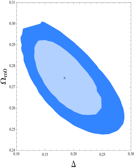
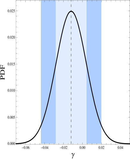
Figure 1: Contour plots for the free parameter $\left\{\Delta-\Omega_{m0}\right\}$ at $1\sigma$ and $2\sigma$ CL for Model I, from the joint analysis $SNIa+BAO+H(z)$ (left panel). Additionally, we present the corresponding marginalized one-dimensional posterior distributions for $\gamma$ parameter (right panel).

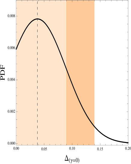
Figure 2: Marginalized one-dimensional posterior distributions for $\Delta_{(\gamma=0)}$ parameter at $1\sigma$ and $2\sigma$ CL for Model II, from the joint analysis $SNIa+BAO+H(z)$.

Table 2 summarizes the main results of the statistical analysis carried out by using the data sets SNIa, SNIa + BAO, and SNIa + BAO + $H(z)$ for two scenarios including i) the Rényi entropy is taking into account within Rastall framework (Model I), and ii) the particular case of $\gamma=0$ (Model II). The parameter $\Omega_{m0}$ takes into account the content of cold dark matter plus baryons to the present. It is useful to note that SNIa does not constrain $\Delta$ very well, and in fact, results are improved by introducing the other observational tests including $BAO$ and $H(z)$. We can also see that the sign change of $\gamma$ does not affect the main thermodynamic consideration obtained from Eq. (4). Indeed, since its obtained values meet the $\gamma<\frac{1}{6}$ condition, entropy is always positive and dynamics, i.e. the acceleration of the universe, is in agreement with the observational data, an outcome in agreement with the results of previous section. For Model I, the likelihood contours arisen from the fitting analysis for the set of free parameters ($\Delta$, $\Omega_{m0}$), and marginalized one-dimensional posterior distributions for $\gamma$ (PDF), considering the best fit values for used data sets $SNIa+BAO+H(z)$, are presented in Fig. 1. Moreover, Fig. 2. includes marginalized one-dimensional posterior distributions for $\Delta_{(\gamma=0)}$ parameter in Model II. Here, we can appreciate slight deviations from the standard model (or equally the $\Delta_{(\gamma=0)}\rightarrow 0$ limit). This possibility does not rule out the standard model, and may in principle be used to distinguish between the $\Lambda CDM$ and our models.

The equation of state (EoS) considering a given cosmological model can be written as

$$w(z)=-1-\frac{2}{3}\frac{\dot{H}}{H^{2}}=-1+\frac{2(1+z)}{3H}\frac{dH}{dz},$$ (77)

which has been derived from the combination of Eqs. (30) and (31), for the general case and Eq. (40) for the particular case of $\gamma=0$. Fig. 3. shows the behavior of the total EoS for both cases, with error propagation at 68.27% CL regarding the best fit values presented in table 2. We note that the total EoS, due to the mechanism presented in this paper, does not cross the phantom division line for the best fit of parameters. To high redshift approach asymptotically to a value of zero, that is, behaving like a fluid without pressure. In general, we note the behavior $-1\lesssim w\lesssim 0$ from the best fit values. Similar behavior are found in unification models in the dark sector of the universe.

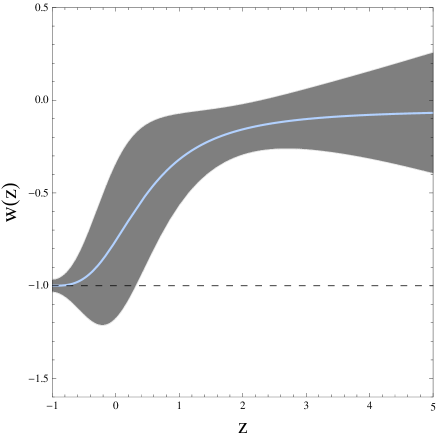
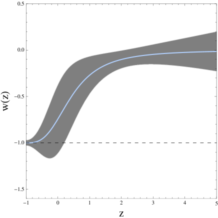
Figure 3: Reconstruction of the EoS at 68% CL (gray region) from our joint analysis Model I (top panel) and Model II ($\gamma=0$) (bottom panel). The blue line represents the best fit value for all data set $SNIa+BAO+H(z)$.

On the other hand, it is natural to describe the kinematics of the cosmic expansion through the Hubble parameter $H(t)$, and its dependence on time, i.e. the deceleration parameter $q(z)$. The deceleration parameter is defined as $q(z)=-\ddot{a}a/\dot{a}$ combined with the $\ddot{a}/a=H^{2}+\dot{H}$ relation, where $\dot{H}=dH/dt$, to get

$$q(z)=-1+\frac{(1+z)}{H(z)}\frac{dH(z)}{dz}.$$ (78)

From Eq. (41) and by considering $p=0$ along with $p^{\gamma}_{e}=-\rho^{\gamma}_{e}$, it follows that

$$q_{0}=\frac{\Omega_{m0}}{2}-\Omega^{\gamma}_{e}$$ (79)

where its RHS has to be evaluated at $z=0$, and we have defined $\Omega^{\gamma}_{e}=\rho^{\gamma}_{e}/\rho_{cr}$. In general, if $\Omega^{\gamma}_{e}$ is sufficiently large (i.e. $\Omega^{\gamma}_{e}>\Omega_{m}$), then $q(z=0)<0$, which corresponds to an accelerated expanding universe.

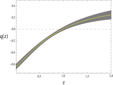
Figure 4: Reconstruction of the $q(z)$ parameter, along with the $1\sigma$ errors (shaded region). From our joint analysis Model I (top panel) and Model II ($\gamma=0$) (bottom panel). The yellow line represents the best fit value for all data set $SNIa+BAO+H(z)$.

$q(z)$ has been plotted in Fig. 4. by using the best fit of parameters with all observational data $SNIa+BAO+Hz$ (See Table 2). As expected, models give $q(z)<0$ at late times and $q(z)>0$ at earlier epoch, which means that the expansion rate is slowed down in past and speeded up at present. Therefore, there is a transition between decelerated phase ($q(z)>0$) into an accelerated era $q(z)<0$ at redshift $z_{t}$ for these models. Our analysis admits $\left\{z_{t}=0.98,q_{0}=-0.63\right\}$ for Model I, and $\left\{z_{t}=0.77,q_{0}=-0.59\right\}$ for Model II.

Data	$\chi^{2}_{min}$	$\Delta$	$\Omega_{m0}$	$\gamma$	$\Omega_{C}$
SNIa	562.227	$0.001\pm 1.702$	$0.279\pm 0.033$	$0.001\pm 0.031$	$0.77\pm 0.36$
SNIa+BAO	564.724	$0.034\pm 0.064$	$0.289\pm 0.015$	$-0.021\pm 0.018$	$0.794\pm 0.073$
SNIa+BAO+H(z)	583.613	$0.183\pm 0.053$	$0.274\pm 0.013$	$-0.012\pm 0.016$	$0.725\pm 0.065$
Model II	Data	$\chi^{2}_{min}$	$\Delta_{(\gamma=0)}$	$\Omega_{m0}$	$\Omega_{C_{(\gamma=0)}}$
$\gamma=0$	SNIa	562.228	$0.02\pm 1.26$	$0.28\pm 0.14$	$0.72\pm 0.15$
$\gamma=0$	SNIa+BAO	564.818	$0.040\pm 0.060$	$0.287\pm 0.013$	$0.713\pm 0.014$
$\gamma=0$	SNIa+BAO+H(z)	585.158	$0.038\pm 0.051$	$0.270\pm 0.010$	$0.729\pm 0.010$

Table 2: Summary of the best fit values at 68.27% CL for the parameters $\Delta(\equiv\frac{(6\gamma-1)\delta\pi}{(4\gamma-1)G})$, $\Omega_{m0}$ and $\gamma$ to Rényi entropy. Also, we shows the summary of the best fit values at 68.27% CL for the particular case where $\gamma=0$, where $\Delta=\Delta_{(\gamma=0)}$. We also present the value of $\Omega_{c}$, derived from standard error propagation.

VI Summary and Concluding Remarks

Applying the Clausius relation, the Cai-Kim temperature and the Rényi entropy to the apparent horizon of flat FRW universe, we could get a model for the dynamics of universe. Fitting model to observational data, the values of model parameters were obtained. We found out that if we attribute Rényi entropy to horizon, then the current accelerated phase of the universe expansion may be described in the Rastall framework. Our study also shows that the probable non-extensive features of spacetime may play the role of a varying dark energy in a universe in which ordinary energy-momentum conservation law is valid.

Although our model shows a suitable agreement with observational data, it is very important to study the evolution of density perturbations in this model which helps us to decide about the performance of our model. We leave this subject for the future work.

References

- (1) P. Rastall, Phys. Rev. D 6, 3357 (1972).
- (2) T. Koivisto, Class. Quant. Grav. 23, 4289 (2006).
- (3) O. Bertolami, C. G. Boehmer, T. Harko, F. S. N. Lobo, Phys. Rev. D 75, 104016 (2007).
- (4) T. Harko and F. S. N. Lobo, Galaxies, 2, 410 (2014).
- (5) H. Moradpour, Y. Heydarzade, F. Darabi, I. G. Salako, Eur. Phys. J. C 77, 259 (2017).
- (6) T. Josset, A. Perez, Phys. Rev. Lett. 118, 021102 (2017).
- (7) H. Shabani, A. H. Ziaie, Eur. Phys. J. C 77, 282 (2017).
- (8) H. Shabani, A. H. Ziaie, Eur. Phys. J. C 77, 507 (2017).
- (9) C. E. M. Batista, M. H. Daouda, J. C. Fabris, O. F. Piattella, D. C. Rodrigues, Phys. Rev. D 85, 084008 (2012).
- (10) V. Dzhunushaliev, H. Quevedo, Gravitation and Cosmology, 23, 280 (2015).
- (11) A. S. Al-Rawaf, M. O. Taha, Phys. Lett. B 366, 69 (1996.
- (12) A. S. Al-Rawaf, M. O. Taha, Gen. Rel. Grav. 28, 935 (1996).
- (13) A.-M. M. Abdel-Rahman, Gen. Rel. Grav. 29, 10 (1997).
- (14) L. L. Smalley, Il Nuovo Cimento B, 80, 1, 42 (1984).
- (15) R. V. dos Santos, J. A. C. Nogales, arXiv:1701.08203v1.
- (16) C. E. M. Batista, J. C. Fabris, O. F. Piattella, A. M. Velasquez-Toribio, Eur. Phys. J. C 73, 2425 (2013).
- (17) T. R. P. Caramês, M. H. Daouda, J. C. Fabris, A. M. Oliveira, O. F. Piattella, V. Strokov, Eur. Phys. J. C 74, 3145 (2014).
- (18) J. C. Fabris, O. F. Piattella, D. C. Rodrigues, C. E. M. Batista, M. H. Daouda, Int. J. Mod. Phys. Conf. Ser. 18, 67 (2012).
- (19) J. P. Campos, J. C. Fabris, R. Perez, O. F. Piattella, H. Velten, Eur. Phys. J. C 73, 2357 (2013).
- (20) J. C. Fabris, M. H. Daouda, O. F. Piattella, Phys. Lett. B 711, 232 (2012).
- (21) K. A. Bronnikov, J. C. Fabris, O. F. Piattella and E. C. Santos, Gen. Relativ. Gravit. 48, 162 (2016).
- (22) I. G. Salako, A. Jawad, Astrophys. Space. Sci. 46, 359 (2015).
- (23) G. F. Silva, O. F. Piattella, J. C. Fabris, L. Casarini, T. O. Barbosa, Gravitation and Cosmology, 19, 156 (2013).
- (24) Y. Heydarzade, F. Darabi, Phys. Lett. B 771, 365 (2017).
- (25) H. Moradpour, Phys. Lett. B 757, 187 (2016) arXiv:1601.04529v6.
- (26) H. Moradpour, I. G. Salako, AHEP, 2016, 3492796 (2016).
- (27) F. F. Yuan, P. Huang, Class. Quantum Grav. 34, 077001 (2017).
- (28) H. Moradpour, N. Sadeghnezhad, S. H. Hendi, Can, Jour. Phys. DOI:10.1139/cjp-2017-0040 arXiv:1606.00846v3.
- (29) I. Licata, H. Moradpour, C. Corda, Int. J. Geom. Methods Mod. Phys. 14, 1730003 (2017).
- (30) A. M. Oliveira, H. E. S. Velten, J. C. Fabris, L. Casarini, Phys. Rev. D 92, 044020 (2015).
- (31) V. G. Czinner, H. Iguchi, Phys. Lett. B 752, 306 (2016).
- (32) C. Corda, J. High Energy Phys. 08, 101 (2011).
- (33) H. Saida, Entropy 13, 1611 (2011).
- (34) G. ’t Hooft, Nucl. Phys. B 256, 727 (1985).
- (35) G. ’t Hooft, Nucl. Phys. B 355, 138 (1990).
- (36) L. Susskind, Phys. Rev. Lett. 71, 2367 (1993).
- (37) J. Maddox, Nature 365, 103 (1993).
- (38) M. Srednicki, Phys. Rev. Lett. 71, 666 (1993).
- (39) A. Strominger, C. Vafa, Phys. Lett. B 379, 99 (1996).
- (40) J. Maldacena, A. Strominger, J. High Energy Phys. 2, 014 (1998).
- (41) S. Das, S. Shankaranarayanan, Phys. Rev. D 73, 121701(R) (2006).
- (42) R. Brustein, M. B. Einhorn, A. Yarom, J. High Energy Phys. 01, 098 (2006).
- (43) L. Borsten, D. Dahanayake, M. J. Duff, H. Ebrahim, W. Rubens, Phys. Rep. 471, 113 (2009).
- (44) H. Casini, Phys. Rev. D 79, 024015 (2009).
- (45) L. Borsten, D. Dahanayake, M. J. Duff, A. Marrani, W. Rubens, Phys. Rev. Lett. 105, 100507 (2010).
- (46) S. Kolekar, T. Padmanabhan, Phys. Rev. D 83, 064034 (2011).
- (47) C. J. Feng, X. Z. Li and X.Y. Shen. Mod. Phys. Lett. A 27, 1250182 (2012).
- (48) A. Sheykhi, Can. J. Phys. 92, 529 (2014).
- (49) H. Moradpour, M. T. Mohammadi Sabet and A. Ghasemi, Mod. Phys. Lett. A 30, 1550158 (2015).
- (50) H. Ebadi and H. Moradpour, Int. J. Mod. Phys. D 24, 1550098 (2015).
- (51) S. Mitra, S. Saha and S. Chakraborty, AOP, DOI: 10.1016/j.aop.2015.01.025 (2015).
- (52) S. Mitra, S. Saha and S. Chakraborty, Gen. Relativ. Gravit. 47, 69 (2015).
- (53) S. Mitra, S. Saha and S. Chakraborty, AHEP. 2015, 430764 (2015).
- (54) S. Mitra, S. Saha and S. Chakraborty, Gen Relativ. Gravit. 47, 38 (2015).
- (55) H. Moradpour and M. T. Mohammadi Sabet, Can. J. Phys. 94, 1 (2016).
- (56) H. Moradpour, R. Dehghani, AHEP. 2016, 7248520 (2016).
- (57) H. Moradpour, N. Sadeghnezhad, S. Ghaffari, A. Jahan, AHEP. 2017, 9687976 (2017).
- (58) H. Moradpour, A. Sheykhi, N. Riazi, B. Wang, AHEP. 2014, 718583 (2014).
- (59) H. Moradpour, R. C. Nunes, E. M. C. Abreu, J. A. Neto, Mod. Phys. Lett. A 32, 1750078 (2017).
- (60) A. Rényi, Probability Theory (North-Holland, Amsterdam, 1970).
- (61) C. Tsallis, J. Stat. Phys. 52, 479 (1988).
- (62) T. S. Biró, V.G. Czinner, Phys. Lett. B 726, 861 (2013).
- (63) C. Tsallis, L. J. L. Cirto, Eur. Phys. J. C 73, 2487 (2013).
- (64) E. M. C. Abreu, J. Ananias Neto, A. C. R. Mendes, W. Oliveira, Physica. A 392, 5154 (2013).
- (65) E. M. C. Abreu, J. Ananias Neto. Phys. Lett. B 727, 524 (2013).
- (66) E. M. Barboza Jr., R. C. Nunes, E. M. C. Abreu, J. A. Neto, Physica A: Statistical Mechanics and its Applications, 436, 301 (2015).
- (67) R. C. Nunes, et al. JCAP, 08, 051 (2016).
- (68) N. Komatsu, S. Kimura. Phys. Rev. D 88, 083534 (2013).
- (69) N. Komatsu, S. Kimura. Phys. Rev. D 89, 123501 (2014).
- (70) N. Komatsu, S. Kimura. Phys. Rev. D 90, 123516 (2014).
- (71) O. Kamel and M. Tribeche, Ann. Phys. 342, 78 (2014).
- (72) H. Moradpour, Int. Jour. Theor, Phys. 55, 4176 (2016).
- (73) N. Komatsu, S. Kimura. Phys. Rev. D 93, 043530 (2016).
- (74) N. Komatsu, Eur. Phys. J. C 77, 229 (2017).
- (75) H. Moradpour, A. Sheykhi, C. Corda, I. G. Salako, Under review in PRD.
- (76) T. Padmanabhan, arXiv:1206.4916 [hep-th].
- (77) M. Akbar, R. G. Cai, Phys. Rev. D 75, 084003 (2007).
- (78) R. G. Cai, S. P. Kim, JHEP 0502, 050 (2005).
- (79) S. Abe, Physica A 368, 430 (2006).
- (80) R. G. Cai, L. M. Cao, Y. P. Hu, Class. Quantum. Grav. 26, 155018 (2009).
- (81) P. Wang, Phys. Rev. D 72, 024030 (2005).
- (82) A. Bialas, W. Czyz, EPL 83, 60009 (2008).
- (83) W. Y. Wen, Int. J. Mod. Phys. D 26, 1750106 (2017).
- (84) V. G. Czinner, H. Iguchi, Universe 3(1), 14 (2017).
- (85) A. Dey, P. Roy, T. Sarkar, [arXiv:1609.02290v3].
- (86) M. Roos, Introduction to Cosmology (John Wiley and Sons, UK, 2003)
- (87) F. Beutler, C. Blake, M. Colless, D. H. Jones, L. Staveley-Smith, L. Campbell, Q. Parker, W. Saunders and F. Watson, MNRAS 416, 3017 (2011).
- (88) C. Blake, T. Davis, G. B. Poole, et al., MNRAS 415, 2892 (2011)
- (89) A. Albrecht, et. al., arXiv:0901.0721
- (90) R. Andrae, T. Schulze-Hartung, & P. Melchior, arXiv:1012.3754 (2010)
- (91) L. Anderson et al., MNRAS 441, 24 (2014).
- (92) A. Font-Ribera, et al., JCAP 1405, 027 (2014).
- (93) D. J. Eisenstein, W. Hu, ApJ, 496, 605 (1998)
- (94) D. J. Eisenstein, et. al., APJ, 633, 560 (2005).
- (95) N. Suzuki, et. al., APJ, 746, 85 (2012).
- (96) R. C. Nunes and D. Pavon. Phys. Rev. D 91 (2015) 063526, arXiv:1503.04113 [gr-qc].
- Nesseris & Perivolaropoulos (2005) S. Nesseris, & L. Perivolaropoulos, 2005, Phys. Rev. D, 72, 123519
- (98) X. L. Meng, X. Wang, S. Y. Li, and T. J. Zhang,
- (99) W. J. Percival et al., 2010, MNRAS, 401, 2148
- (100) L. Wolz, M. Kilbinger, J. Weller, and T. Giannantonio, JCAP 9, 009 (2012).