Sparse Variable Selection on High Dimensional Heterogeneous Data with Tree Structured Responses

Abstract

We consider the problem of sparse variable selection on high dimension heterogeneous data sets, which has been taken on renewed interest recently due to the growth of biological and medical data sets with complex, non-i.i.d. structures and prolific response variables. The heterogeneity is likely to confound the association between explanatory variables and responses, resulting in a wealth of false discoveries when Lasso or its variants are naïvely applied. Therefore, the research interest of developing effective confounder correction methods is growing. However, ordinarily employing recent confounder correction methods will result in undesirable performance due to the ignorance of the convoluted interdependency among the prolific response variables. To fully improve current variable selection methods, we introduce a model that can utilize the dependency information from multiple responses to select the active variables from heterogeneous data. Through extensive experiments on synthetic and real data sets, we show that our proposed model outperforms the existing methods.

1 INTRODUCTION

Variable selection is one of the central tasks in statistics and has been studied for decades (?; ?; ?). Modern machine learning problems, especially biological or medical applications often seek for solutions in the existing statistical approaches. Lasso (?) is an example of those extensively adopted methods in a variety of areas for sparse variable selection tasks. However, the increasing volume of data sets often requires the data to be collected from multiple batches and then integrated together. This procedure is particularly harmful to the biological (?) and medical (?; ?) data sets, which are sensitive to the data sources, like populations, hospitals or even experimental devices. This sensitivity results in heterogeneity, therefore, breaks one of the most fundamental assumptions (i.i.d. assumption) that most statistical machine learning methods make. More importantly, due to the expensiveness of biological and medical data, different batches of data are collected for different purposes from distinctly different sources. Consequently, the heterogeneity often induces confounding factors between explanatory variables and response variables, resulting in numerous false positive selected variables when classical variable selection methods are applied (?).

To further understand the challenge heterogeneity introduces to biological or medical data sets and define the problem, consider that we have data samples in the format of $(X,Z,Y)$, where $X$ stands for the explanatory variables, $Y$ stands for the responses, and $Z$ stands for the indicator of the data source. The dependency between $X$ and $Y$ is the premise of any variable selection task (?), and the dependency between $X$ and $Z$ is introduced through heterogeneity (?; ?; ?). More importantly, biological and medical data are typically expensive to collect, therefore, individual samples of certain diseases are mostly collected from the patients of many hospitals, while samples of the control group are mostly collected from volunteers from several different undeveloped regions. This data collection procedure brings the dependency between $Z$ and $Y$.

In the real world, this problem may be even challenging, for the origin of different samples is lost either through data compression or experimental necessity in most cases. Nowadays genetic association studies rarely see the origin of samples listed. $Z$ becomes the confounding factor between $X$ and $Y$ (?). One challenge of the heterogeneous data variable selection problem is to correct the confounding effects introduced by $Z$.

Further, many of the real world biological and medical data sets are collected with multiple response variables. These responses are often more closely related and more likely to share common relevant covariates than others (?; ?). For instances, in genetic association analysis, which aims to select the single-nucleotide polymorphism (explanatory variables) that could affect the phenotype (response variables), the genes that in the same pathway are more likely to share the common set of relevant explanatory variables than other genes. Thus, to improve the performance of the variable selection, incorporating the complex correlation structure in the responses is under our consideration. Therefore, in this paper, we extend the recent solutions of sparse linear mixed model (?; ?) that can correct confounding factors and perform variable selection simultaneously further to account the relatedness between different responses. We propose the tree-guided sparse linear mixed model, namely TgSLMM, to correct the confoundings and incorporate the relatedness among response variables simultaneously. Further, we examine our model through extensive synthetic experiments and show that our method is superior to other existing approaches.

2 RELATED WORK

Recent years have witnessed the great advances in the variable selection area. The most classical approach is $\ell_{1}$-norm regularization (i.e. Lasso regression (?)). Further, recent studies have extended the model capability by introducing different regularizers (?). Examples including the Smoothly Clipped Absolute Deviation (SCAD) (?), the Local Linear Approximation (LLA) (?) and the Minimax Concave Penalty (MCP) (?) have been introduced recently. These methods overcome the limitations of Lasso (?) at the cost of introducing nonconvexity in the optimization problem. Some other variable selection methods like (?) ignore underlying multidimensional structure, leading to severe small dataset problems. (?) imposes a rank constraint into $\ell_{1}$ regularization to factor matrice and promotes sparsity in variable selection, which hurts the interpretability. (?) proposed a unsupervised variable selection method, but cannot apply to high dimensional data with heterogeneity.

In the non-i.i,d setting, such as when the data set is originated from different sources, confounders could raise a challenge in variable selection. Corresponding solutions have been studied for decades. Principal components analysis (PCA) (?; ?) and linear mixed model (?; ?) are two popular and efficient approaches to correct the confounding effect. The latter provides a more fine-grained way to model the population structure and won its prominence in the animal breeding literature, where they were used to correct the kinship and family structure (?). Many extensions have been developed. But these extensions such as LMM-Select (?) LMM-BOLT (?) and Liability-threshold mixed linear model (LTMLM) (?) along with other methods (?; ?; ?) only rely on univariate testing to select the variable once the confounding factor is corrected. Recent attempts have been made to propose multi-variable testing model (?; ?; ?; ?).

3 TREE-GUIDED SPARSE LINEAR MIXED MODEL

Throughout this paper, $X$ denotes the $n\times p$ matrix for explanatory variables of each individuals, $Y$ for the $n\times k$ matrix for response variables, and $\beta$ for the $p\times k$ effect sizes. We use subscripts to denote rows and superscripts to denote columns, for example, $\beta_{k}$ and $\beta^{k}$ is the $k$-th column and $k$-th row of $\beta$ respectively.

3.1 Sparse Linear Mixed Model

The linear mixed model (LMM) is an extension of the standard linear regression model that explicitly describes the relationship between a response variable and explanatory variables incorporating an extra random term to account for confounding factors. To introduce sparse linear mixed model (LMM-Lasso), we briefly revisit the classical linear mixed model as Equation 1:

$$Y=X\beta+Zu+\epsilon$$ (1)

where $Z$ is a $n\times t$ matrix of random effect, $u$ is confounding influences and $\epsilon$ denotes observation noise and they all follow the Gaussian distribution with the zero means. Intuitively, the product $Zu$ models the covariance between the observations $y_{i}$. Assuming that $\epsilon\sim\,\mathcal{N}(\,0,\,\sigma_{\epsilon}^{2}I)$, we can further rewrite the formula as Equation 2 to simplify mathematical derivation:

$$y_{k}\sim\mathcal{N}\,(X\beta_{k},\,\sigma_{g}^{2}K+\sigma_{\epsilon}^{2}I\,)$$ (2)

where $K=ZZ^{T}$, representing the covariance between the responses, $\sigma_{g}$ represents the magnitude of confounder factors. Assuming the priori distribution of $\beta$ could be expressed as $e^{-\Phi(\beta)}$, we can define log likelihood function as Equation 3:

$$\ell(\sigma_{g}^{2},\sigma_{\epsilon}^{2},\beta)=e^{-\Phi(\beta)}\cdot\prod_{k=1}^{K}\mathcal{N}\,(y_{k}|X\beta_{k},\,\sigma_{g}^{2}K+\sigma_{\epsilon}^{2}I\,)$$ (3)

Due to the sparsity of $\beta$, it’s reasonable to assume that $\beta$ follows Laplace shrinkage prior. Such assumption leads to the sparse linear mixed model (LMM-Lasso). However, LMM-Lasso fails to consider the relatedness among response variables. Such defect drives us to the tree-guided sparse linear mixed model.

3.2 Tree-Guided Sparse Linear Mixed Model

Based on the framework of Equation 3， we substitute the above Equation 4 then define Tree-Lasso into Equation 3, we can get the optimization equation for the proposed TgSLMM.

$$\Phi(\beta)=\lambda\sum{j}\sum_{v\in V}w_{v}||\beta_{j}^{G_{v}}||_{2}$$ (4)

where $\lambda$ is a tuning parameter that controls the amount of sparsity in the solution. Tree-Lasso incorporates the relatedness among responses simultaneously as Equation 4. The weights and overlaps of groups of Tree-Lasso are determined by the hierarchical clustering tree (?; ?). Given each node $v\in{V}$ of the $j$-th tree is associated with height $h_{v}$ of the group $G_{v}$ whose members are the response variables at the leaf nodes of the subtree rooted at node $v$. In general, $h_{v}$ represents the weight for selecting relevant covariates separately for the responses associated with each child of node $v$, whereas the $1-h_{v}$ represents the weight for selecting relevant covariates jointly for the responses for all of the children of node $v$. $\beta_{j}^{G_{v}}$ is a vector of regression coefficients $\{\beta_{j}^{k}|k\in G_{v}\}$. Each group of subtree regression coefficients $\beta_{j}^{G_{v}}$ is weighted with $w_{v}$, which is defined as the Equation 5:

$${w_{v}=\left\{\begin{array}[]{rcl}(1-h_{v})\prod\limits_{m\in Ancestors(v)}{h_{m}}&&\mbox{if v is an internal node,}\\ \prod\limits_{m\in Ancestors(v)}{h_{m}}&&\mbox{if v is a leaf node.}\end{array}\right.}$$ (5)

Further, assuming $|V|$ is the number of response variables, which is equivalent to the number of leaf nodes in the tree.

3.3 Parameter Learning

Overall, optimizing Equation 4 with hyper-parameter {$\Theta=\sigma_{g}^{2},\,\sigma_{\epsilon}^{2},\,\lambda,\,w_{v}$} is a non-convex optimization problem aside with weight $\beta$. Hence, we use the null-model fitting method first to correct the confounding factors without the consideration of fixed effect, and then solve Tree-Lasso regression problem using smoothing proximal gradient method (?).

Null-model

Null-model fitting method by first optimizing $\sigma_{g}^{2}$, $\sigma_{\epsilon}^{2}$ under null model while ignoring the fixed effect of explanatory variables, can yield near-identical result as an exact method (?). Introducing the ratio of the random effect and the noise variance, $\delta=\sigma_{\epsilon}^{2}/\sigma_{g}^{2}$, we could transform the equation as Equation 6:

$$\ell_{null}(\sigma_{g},\delta)=e^{-\Phi(\beta)}\cdot\prod_{k=1}^{K}\mathcal{N}\,(y_{k}|X\beta_{k},\,\sigma_{g}^{2}(K+\delta{I})$$ (6)

In general, we first compute the spectral decomposition of $K=Udiag(d)U^{T}$, where $U$ for eigenvector matrix and $diag(d)$ for eigenvalue matrix. After that, we rotate the data in order to make the covariance of the Gaussian distribution isotropic. Then, we carry out a one-dimension optimization with regard to $\delta$ to optimize the log-likelihood, while $\sigma_{g}$ can be optimized in closed form in every evaluation.

Reduction to Tree-Lasso regression problem

Having the yielded $\delta$, we use the $U$ computed before to rotate the data such that the covariance matrix becomes isotropic. Assume $\tilde{Y}$ and $\tilde{X}$ are the resulting rescaled data, which can be calculated by following equation:

$$\tilde{X}=(diag(d)+\delta{I})^{-\frac{1}{2}}U^{T}X$$

$$\tilde{Y}=(diag(d)+\delta{I})^{-\frac{1}{2}}U^{T}Y$$

Using this transformation, the equation eventually ends up with a standard Tree-Lasso regression problem since it is free of population structure. Thus in the following step, we can obtain the $\widehat{\beta}^{tree}$ as Equation 7:

$$\widehat{\beta}^{tree}=\min\limits_{\beta}\frac{1}{2}||\tilde{Y}-\tilde{X}\beta||_{F}^{2}+\Phi(\beta)$$ (7)

where $||\cdot||_{F}$ denotes the matrix Frobenius norm, and $\Phi$ is determined by the Equation 4, then we can easily employ the smoothing proximal gradient descent method.

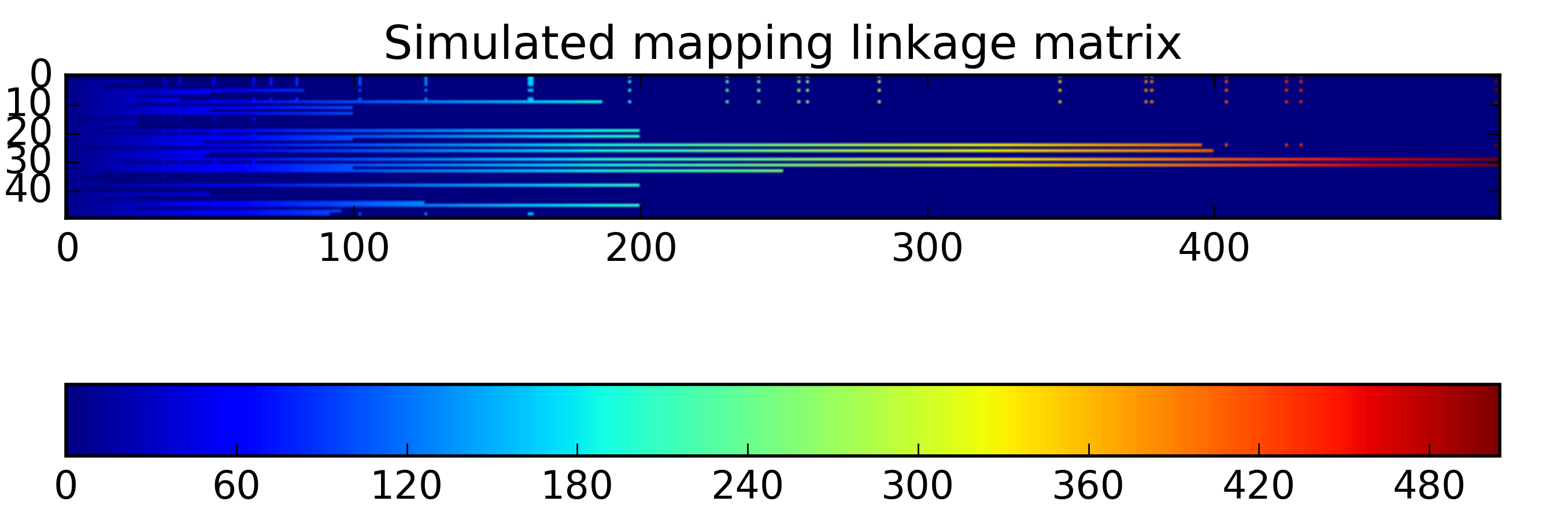
Figure 1: The simulated ground-truth $\beta$ vector. For illustration purpose, we choose the experimental setting of $n=250$, $p=500$ and $k=50$.

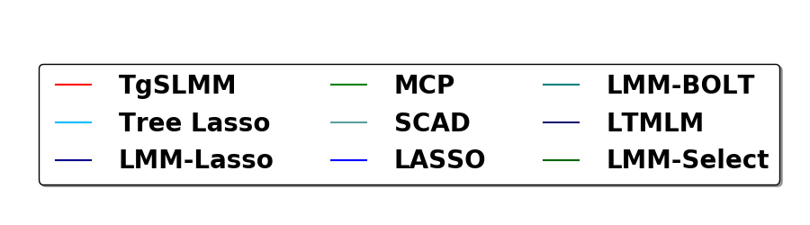
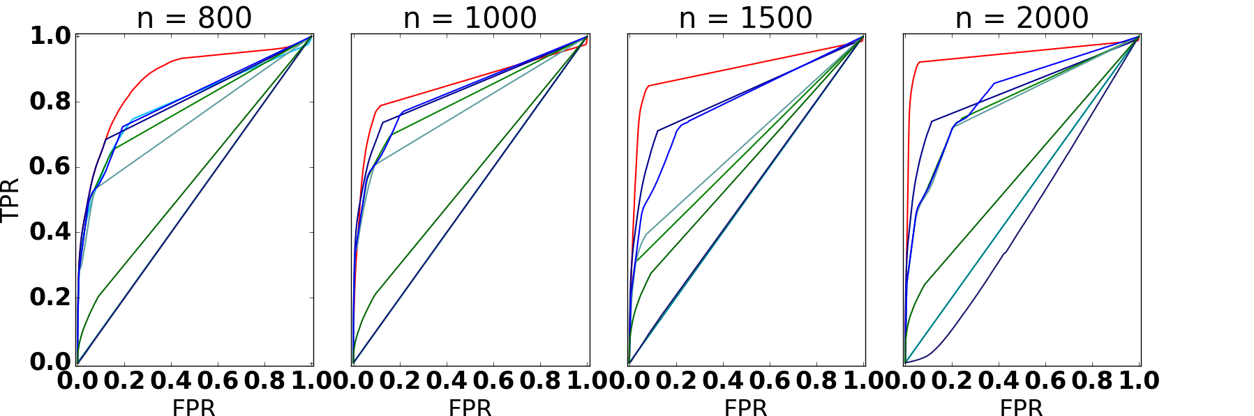
(a) Different number of samples

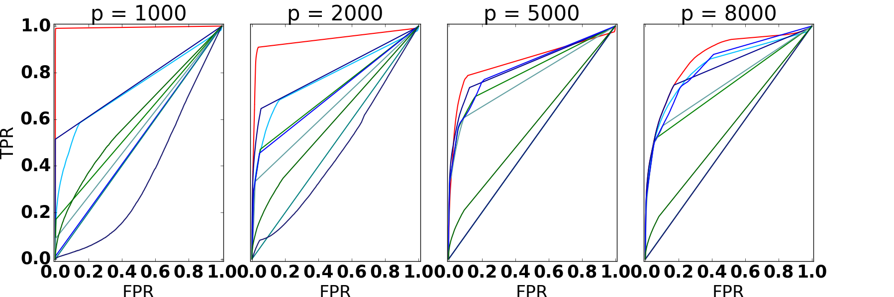
(b) Different number of explanatory variables

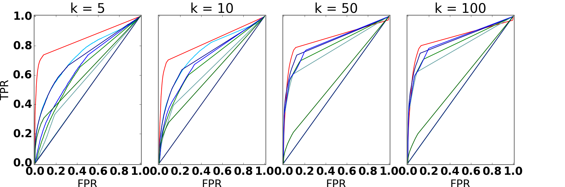
(c) Different number of response variables

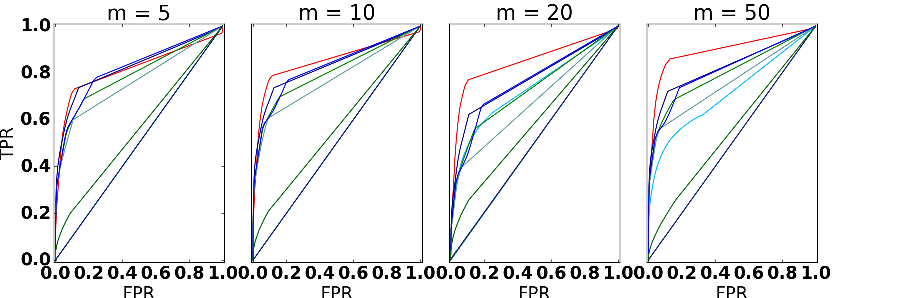
(d) Different number of distributions

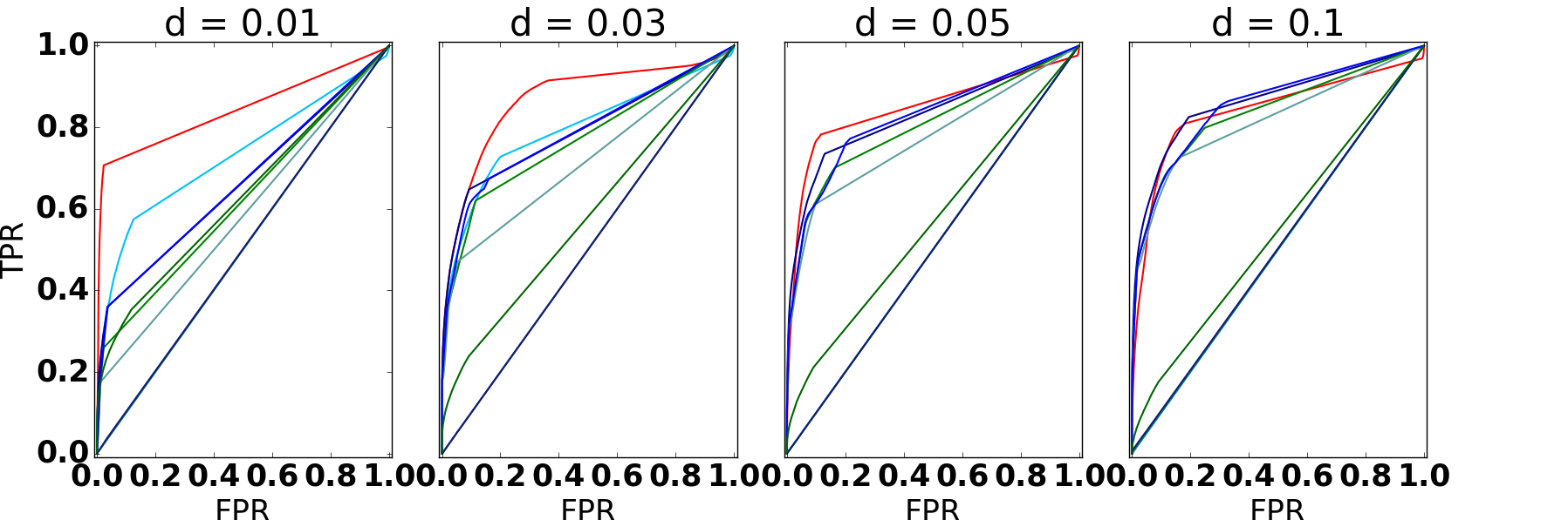
(e) Different percentage of active variables

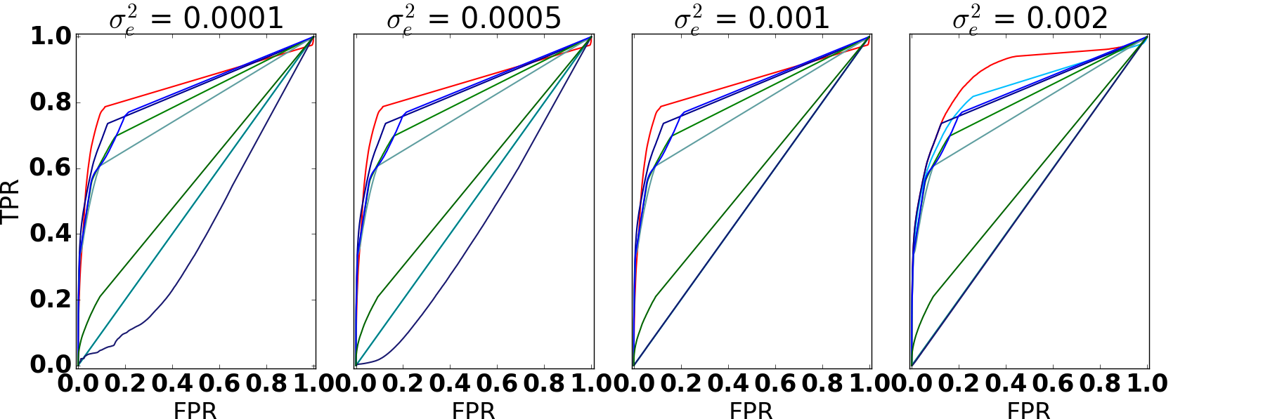
(f) Different magnitude of variance of explanatory variables

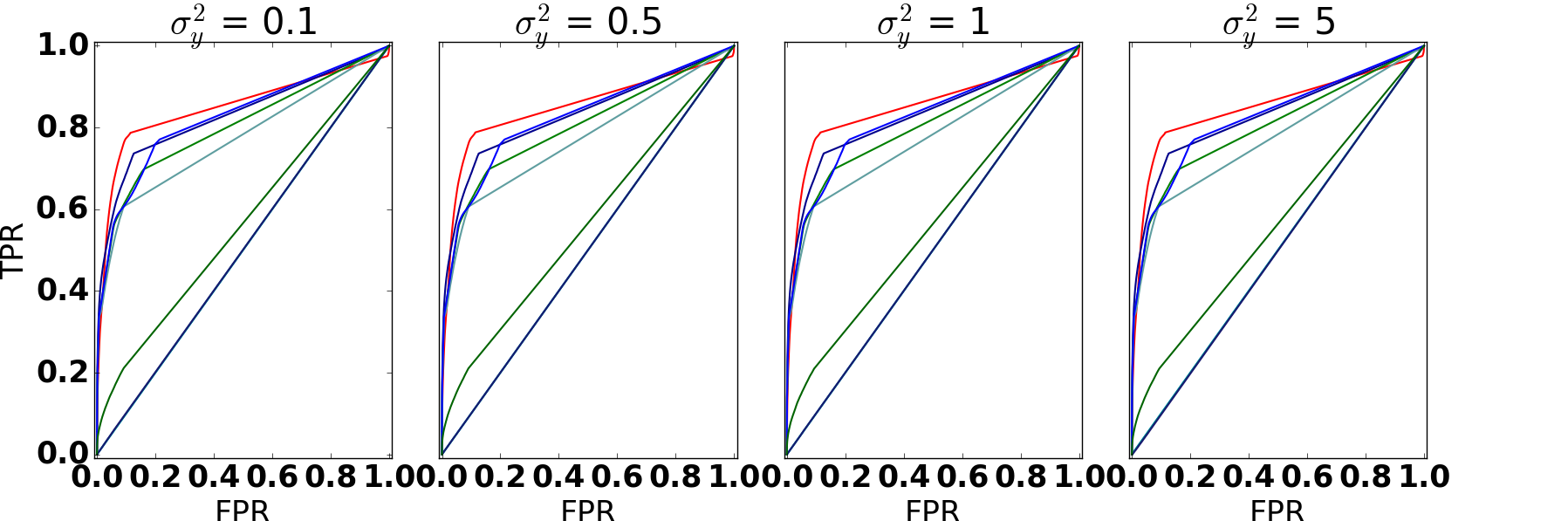
(g) Different magnitude of variance of response variables

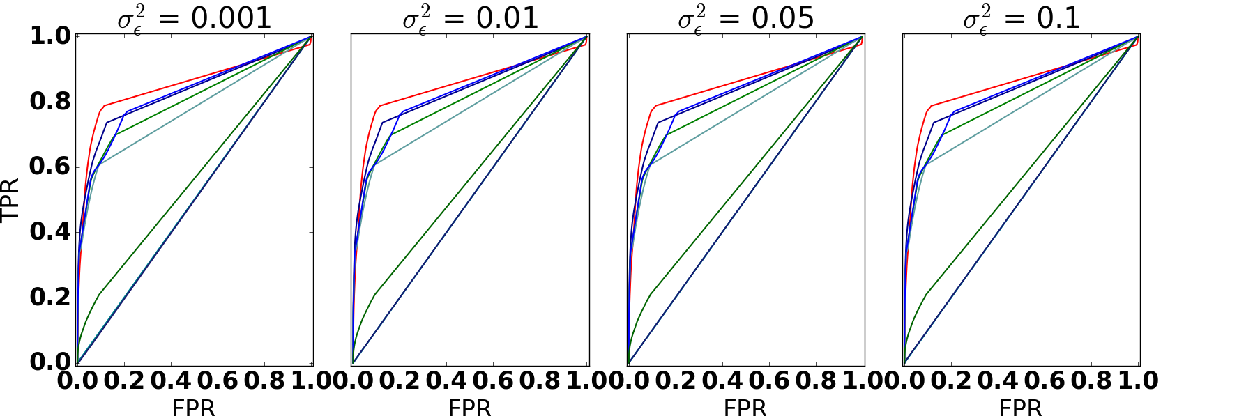
(h) Different magnitude of noise

Figure 2: ROC curves for experiments with different parameters. We show the full image of ROC curves to compare our method with previous methods. For each configuration, the reported curve is drawn over five random seeds.

4 SYNTHETIC EXPERIMENTS

In this section, we evaluate the yielded results of the TgSLMM versus Tree-Lasso, LMM-Lasso and some methods mentioned above, which are shown in the receiver operating characteristic (ROC) curves .

4.1 Data Generation

First, we simulate a sparse tree-structured vector as $\beta$. An illustrated example is shown in Figure 1. Each row of $\beta$ can be viewed as either a leaf node with elements shattered in different columns, or a non-leaf node, which contains all elements its child node holds. The generation rules are listed below:

• The righter columns have fewer non-zero elements

• The elements from righter columns have bigger value.

• The leftmost column has non-zeros elements in all positions, which denotes the most general feature.

• The non-leaf nodes can be iteratively divided into two different kinds of nodes. One has non-zeros elements in all column while the other one only has non-zeros elements in the rightest column.

Then we generate centroids of $m$ different distributions. $c_{j}$ is the centroid of $j$-th distribution, we generate explanatory variable data from a multivariate Gaussian distribution as follows:

$$x_{i}\sim\mathcal{N}\,(c_{j},\,\sigma_{e}^{2}{I})$$ (8)

where $x_{i}$ denotes the i-th data and originates from j-th distribution. Then we generate an immediate response vector $r$ from $X$ vector with $\epsilon\sim\,(0,\sigma_{\epsilon}^{2})$:

$$r=X\beta+\epsilon$$ (9)

To get the final response vector $Y$, we introduce a covariance matrix $K$ to simulate correlation between different responses:

$$Y\sim\mathcal{N}\,(r,\,\sigma_{y}^{2}K)$$ (10)

where $\sigma_{y}^{2}$ is to control the magnitude of the variance. Assuming $C$ is the matrix formed by stacking the centroids $c_{j}$, we choose $K=CC^{T}$ to simulate the correlation between observations.

4.2 Experiment Results

We assessed the ability of TgSLMM in our synthetic datasets. The experimental setting is listed in Table 1.

Table 1: Default experimental setting in the simulated experiments

Parameter	Default	Description
$n$	1000	the number of data samples
$p$	5000	the number of explanatory variables
$k$	50	the number of response variables
$m$	10	the number of distributions that data originates from
$d$	0.05	the percentage of active variables
$\sigma_{e}^{2}$	0.001	the magnitude of covariance of explanatory variables
$\sigma_{y}^{2}$	1	the magnitude of covariance of response variables
$\sigma_{\epsilon}^{2}$	0.05	the magnitude of noise

The results are shown in Figure 2. To evaluate the performance of the proposed model, Tree-Lasso, LMM-Lasso, MCP, SCAD, Lasso, BOLT-LMM, LTMLM and LMM-Select are also tested. In general, our method outperforms all the other methods.

We examine each method’s ability to identify active variables in different datasets by modifying each default values. In Figure 2(a) as $n$ increases, and in Figure 2(b) as $p$ decreases, the ratio of $\frac{p}{n}$ gets smaller and the performance gets better as expected. Compared to Tree-Lasso along with other methods, our method is more robust with big datasets, which are accord with the real-world situation. As we increase the number of response variables in Figure 2(c), increase the number of distributions in Figure 2(d), or decrease the proportion of active variables in $\beta$ as Figure 2(e), the problem becomes more challenging. Figure 2(f) and Figure 2(g) show that our method is more flexible to different covariance of explanatory variables and response variables. In Figure 2(e), we notice that when the proportion of active variables in $\beta$ is large, the performance of TgSLMM and LMM-Lasso is similar. However, it contradicts the background of our research, that the active variables should be sparse among data. Through our experiments, it is hard for Tree-Lasso to identify the active variables on high dimension heterogeneous data.

TgSLMM also performs best in most cases in the figure of Precision-Recall curves. These figures are omitted to save space.

4.3 Analysis of yielded $\beta$ and $Y$

We use the same experimental setting as in Figure 1. The results are shown in Figure 3 and 4.

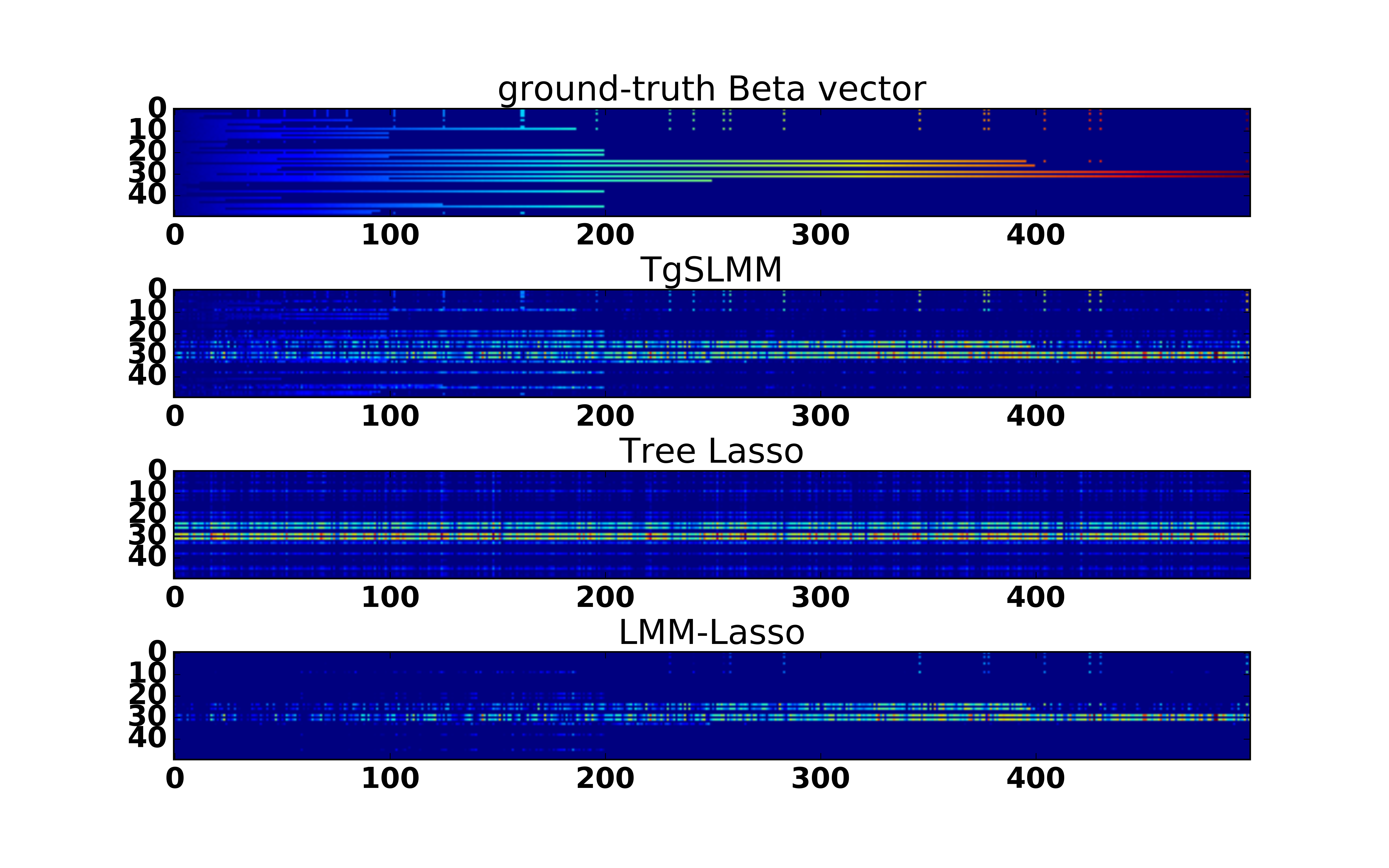
Figure 3: The yielded $\beta$ vector.

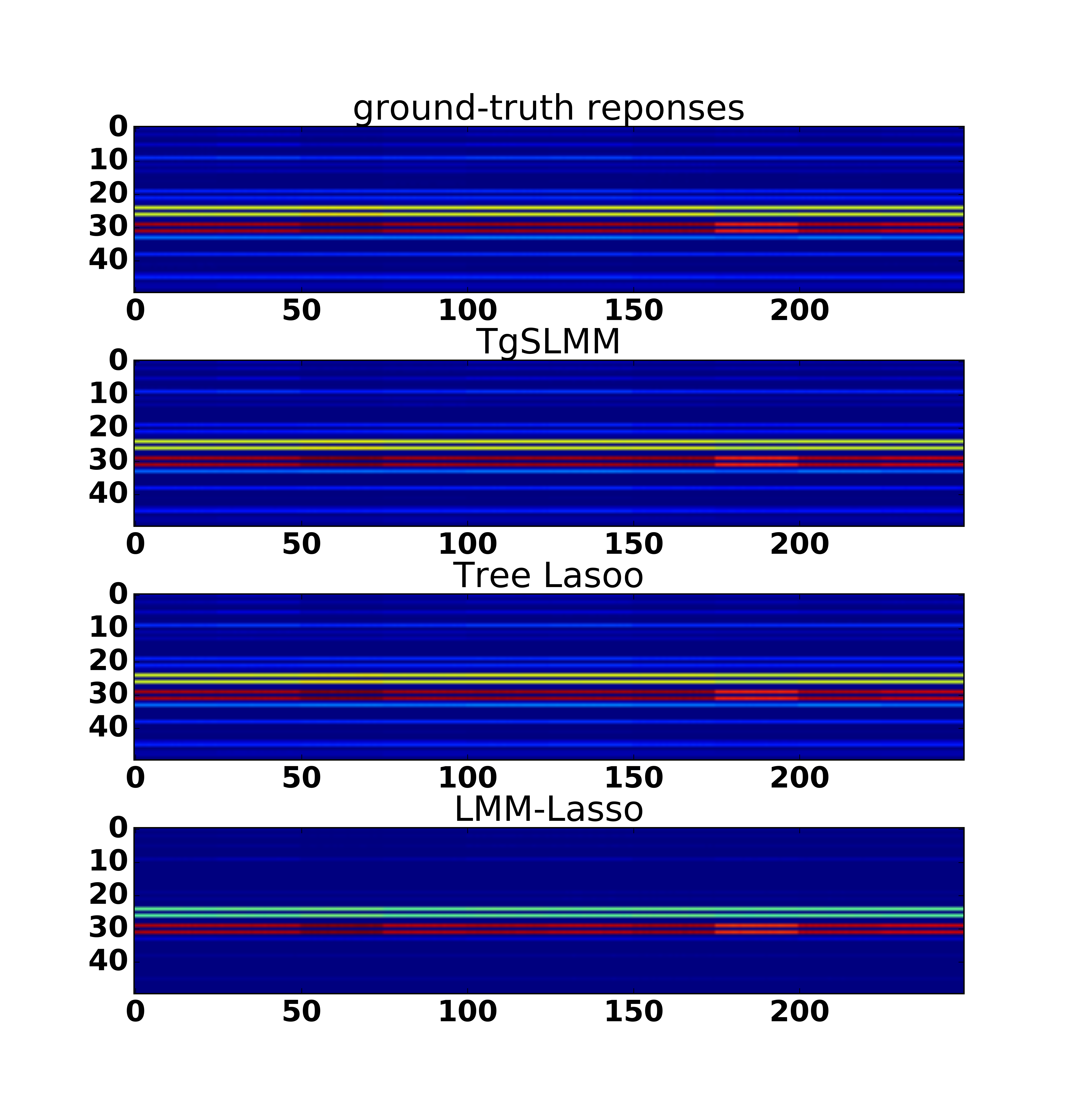
Figure 4: The simulated responses matrix and the predicted responses results by different models.

Figure 3 shows that TgSLMM recovers both the values and structure of ground truth effect size, revealing the supreme ability of TgSLMM in variable selection. LMM-Lasso has trouble finding enough useful information. Trapped into the confounding factors, the Tree-Lasso discovers too many false positives. Tree-Lasso also falls short when the dataset becomes complicated as the dataset we generated in the Figure 2. Based on Figure 4, both prediction performance of TgSLMM and Tree-Lasso are convincing, LMM-Lasso fails as reported before. Unsurprisingly, the proposed TgSLMM also behaves the best in estimating $\beta$ with respect to mean-squared error through almost all experimental settings. The figures of mean-squared error of $\beta$ are omitted, as well as analysis for the other methods. The remaining other approaches cannot discover any meaningful information.

By using the proposed method, we are able to detect weak signals and reveal clear groupings in the patterns of associations between explanatory variables and responses. The results also prove our method does well both in the field of variable selection, effect sizes estimation and response prediction.

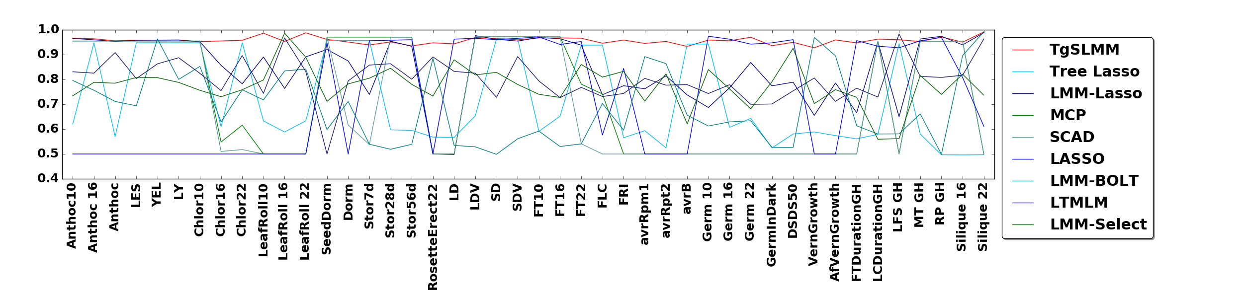
Figure 5: Area under ROC curve for the 44 traits of Arabidopsis thaliana.

5 REAL GENOME DATA EXPERIMENTS

Having shown the capacity of TgSLMM in recovering explanatory variables of synthetic datasets, we now demonstrate how TgSLMM can be used in real-world genome data and discover meaningful information. To evaluate the method, we focus on some practical datasets, Arabidopsis thaliana, Heterogeneous Stock Mice and Human Alzheimer Disease. Since Arabidopsis thaliana and Heterogeneous Stock Mice have been studied for over a decade, the scientific community has reached a general consensus regarding these species (?). With such authentic golden standard, we could plot the ROC curve and assess model’s performance using area under it. However, since Alzheimer’s disease is a very active area of research with no ground truth available, we listed the genetic variables identified by our proposed model and verified the top genetic variables by searching the relevant literature.

5.1 Data Sets

Arabidopsis Thaliana

The Arabidopsis thaliana dataset we obtained is a collection of around 200 plants, each with around 215,000 genetic variables (?). We study the association between these genetic variables and a set of observed responses. These plants were collected from 27 different countries in Europe and Asia, so that geographic origin serves as a potential confounding factor. For example, different sunlight conditions in different regions may affect the observed responses of these plants. We tested the genetic associations between genetic variables with 44 different responses such as days to germination, days to flowering, etc.

Heterogeneous Stock Mice

The heterogeneous stock mice dataset contains measurements from around 1700 mice, with 10,000 genetic variables (?). These mice were raised in cages by four generations over a two-year period. In total, the mice come from 85 distinct families. The obvious confounding variable is genetic inheritance due to family relationships. We studied the association between the genetic variables and a set of 27 response variables that could possibly be affected by inheritance. These 27 response variables fall into six different categories, relating to the glucose level, insulin level, immunity, EPM, FN and OFT respectively.

Human Alzheimer Disease

We use the late-onset Alzheimer’s Disease data provided by Harvard Brain Tissue Resource Center and Merck Research Laboratories (?). It consists of measurements from 540 patients with 500,000 genetic variables. We tested the association between these genetic variables and 28 responses corresponding to a patient’s disease status of Alzheimer’s disease.

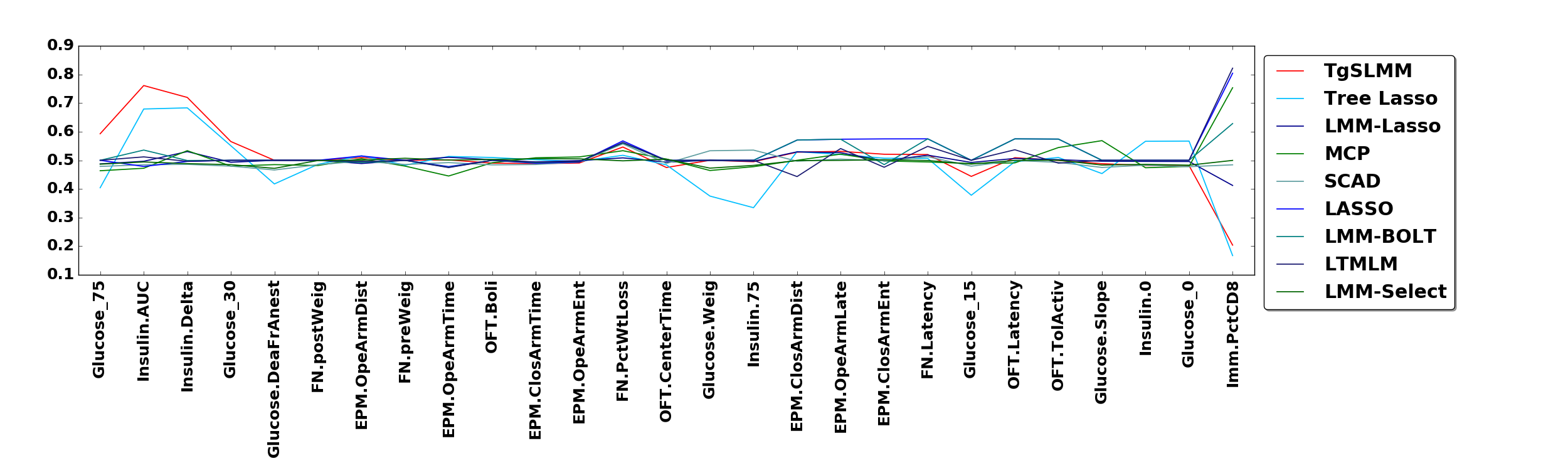
Figure 6: Area under ROC curve for the 27 traits of mice.

5.2 Arabidopsis Thaliana

Since we have access to a validated gold standard of the Arabidopsis thaliana dataset, we compared the alternative methods in terms of their ability in recovering explanatory variables with a true association. Figure 5 illustrates the area under the ROC curve for each response variables for Arabidopsis thaliana. By analyzing the yielded results, it can be concluded that TgSLMM equals or outperforms the other methods for all of responses. We can also reach that TgSLMM allows for dissecting individual explanatory variable effects from global genetic effects driven by population structure.

Further, we applied cross-validation to evaluate the proposed model’s ability of response prediction. Using the data our method selects, 61.4% of prediction for Arabidopsis thaliana is better than using origin dataset, 56.8% is better than employing Tree-Lasso, 79.5% is better than applying LMM-Lasso, 84.1% is better than MCP and SCAD, 66.0% is better than Lasso, 91.0% is better than LMM-BOLT, 56.7% is better than LTMLM. Our method only works worse than LMM-Select while considering prediction.

5.3 Heterogeneous Stock Mice

For Heterogeneous Stock Mice dataset, ground truth is also available so that we could evaluate the methods based on the area under their ROC Curve as Figure 6. TgSLMM behaves as the best one on 22.2% of the traits and achieved the highest area for the whole datasets as 0.627. The second best model is MCP with area of 0.604. The area under ROC of Tree-Lasso, Lasso and SCAD is 0.582, 0.591 and 0.590 respectively. The area of the remaining models is all around 0.5, showing little ability to process such complex datasets. On trait Glucose_75, Glucose_30, Glucose.DeadFromAnesthetic, Insulin.AUC, Insulin.Delta and FN.postWeight, our method TgSLMM behaves best. The results are interesting: The left side of the figure mostly consists of traits regarding glucose and insulin in the mice, while the right side of the figure consists of trait related to immunity. This raises the interesting question of whether or not immune levels in stock mice are largely independent of family origin.

5.4 Human Alzheimer Disease

Finally, we proceed to the Human Alzheimer’s Disease dataset. We report the top 30 genetic variables our model discovered in Table 2 to foster further research.

Table 2: Discovered Genetic Variables with TgSLMM

Rank	SNP	Rank	SNP	Rank	SNP
1	rs30882	11	rs10897029	21	rs2298955
2	rs10027921	12	rs464906	22	rs1998933
3	rs12641981	13	rs874404	23	rs17467420
4	rs12506805	14	rs4421632	24	rs7629705
5	rs684240	15	rs6086773	25	rs27162
6	rs1684438	16	rs4882754	26	rs4740820
7	rs6431428	17	rs2272445	27	rs1495805
8	rs12509328	18	rs12410705	28	rs7916633
9	rs7783626	19	rs4578488	29	rs13221797
10	rs11848278	20	rs3887171	30	rs429536

Due to space limitation, we only verify the top 10 reported genetic variables with prior research. The $1^{st}$ discovered genetic variable is corresponded to apoB gene, which can influence serum concentration in Alzheimer’s disease (?). The $2^{nd}$ one is associated with ARHGAP10 gene (also called GRAF2), which affects the developmentally regulated expression of the GRAF proteins that promote lipid droplet clustering and growth, and is enriched at lipid droplet junctions (?). The $4^{th}$ SNP is expressed by the SYNPO2, which influences hypercholesterolemia or hypertension that has a identified a link between cognitive deficits (?). The $7^{th}$ genetic variable is associated with AGAP1. AGAP1 can regulate membrane trafficking, actin remodeling (?) and is reported to be associated with Alzheimer’s disease. The $8^{th}$ one is coded by gene Fam114a1. Biologists have found that Fam114a1 is highly expressed in the developing neocortex (?). The $9^{th}$ is corresponded with gene CNTNAP2 and the direct downregulation of CNTNAP2 by STOX1A is associated with Alzheimer’s disease(?).

6 CONCLUSION

In this paper, we aim to solve the challenging task of sparse variable selection when the data is not i.i.d. This type of situation often occurs in genomics since different batches of medical data are collected from different sources for different purposes. Due to such confounding factors, naiv̈ely applying the traditional variable selection methods will result in a wealth of false discoveries. In addition to that, existing methods ignore the convoluted interdependency among prolific responses, hence a joint analysis that can utilize such relatedness information in a heterogeneous data set is crucial. To address these problems, we proposed the tree-guided sparse linear mixed model for sparse variable selection in the heterogeneous data set. We extend the recent solutions of LMM that can correct confounding factors and perform variable selection simultaneously further to account the relatedness between different responses. Through extensive experiments, we compare our method with state-of-art methods and deeply analyze how confounding factors from the high dimensional heterogeneous data set influence the capability of the model to identify active variables. We show that traditional methods easily fall into the trap of utilizing false information, while our proposed model outperforms other existing methods in both the synthetic data set and real genome data set.

References

- [Anastasio et al. 2011] Anastasio, A. E.; Platt, A.; Horton, M.; Grotewold, E.; Scholl, R.; Borevitz, J. O.; Nordborg, M.; and Bergelson, J. 2011. Source verification of mis-identified arabidopsis thaliana accessions. The Plant Journal 67(3):554–566.
- [Astle and Balding 2009] Astle, W., and Balding, D. J. 2009. Population structure and cryptic relatedness in genetic association studies. Statistic Sci 451–471.
- [Atwell et al. 2010] Atwell, S.; Huang, Y. S.; Vilhjálmsson, B. J.; Willems, G.; Horton, M.; Li, Y.; Meng, D.; Platt, A.; Tarone, A. M.; Hu, T. T.; et al. 2010. Genome-wide association study of 107 phenotypes in arabidopsis thaliana inbred lines. Nature 465(7298):627–631.
- [Bondell, Krishna, and Ghosh 2010] Bondell, H. D.; Krishna, A.; and Ghosh, S. K. 2010. Joint variable selection for fixed and random effects in linear mixed-effects models. Biometrics 66(4):1069–1077.
- [Cai, Zhang, and He 2010] Cai, D.; Zhang, C.; and He, X. 2010. Unsupervised feature selection for multi-cluster data. In Proceedings of the 16th ACM SIGKDD. ACM.
- [Caramelli et al. 1999] Caramelli, P.; Nitrini, R.; Maranhao, R.; Lourenco, A.; Damasceno, M.; Vinagre, C.; and Caramelli, B. 1999. Increased apolipoprotein b serum concentration in alzheimer’s disease. Acta neurologica scandinavica 100(1):61–63.
- [Chen and Wang 2013] Chen, Q., and Wang, S. 2013. Variable selection for multiply-imputed data with application to dioxin exposure study. Statistics in medicine 32(21):3646–3659.
- [Chen et al. 2010] Chen, X.; Kim, S.; Lin, Q.; Carbonell, J. G.; and Xing, E. P. 2010. Graph-structured multi-task regression and an efficient optimization method for general fused lasso. arXiv preprint arXiv:1005.3579.
- [Chen et al. 2012] Chen, X.; Lin, Q.; Kim, S.; Carbonell, J. G.; and Xing, E. P. 2012. Smoothing proximal gradient method for general structured sparse regression. The Annals of Applied Statistics 719–752.
- [Du and Shen 2015] Du, L., and Shen, Y.-D. 2015. Unsupervised feature selection with adaptive structure learning. In Proceedings of the 21th ACM SIGKDD. ACM.
- [Fan and Li 2001] Fan, J., and Li, R. 2001. Variable selection via nonconcave penalized likelihood and its oracle properties. Journal of the American statistical Association 96(456):1348–1360.
- [Fan and Li 2012] Fan, Y., and Li, R. 2012. Variable selection in linear mixed effects models. Annals of statistics 40(4):2043.
- [Goddard 2009] Goddard, M. 2009. Genomic selection: prediction of accuracy and maximisation of long term response. Genetica 136(2):245–257.
- [Golub et al. 1999] Golub, T. R.; Slonim, D. K.; Tamayo, P.; Huard, C.; Gaasenbeek, M.; Mesirov, J. P.; Coller, H.; Loh, M. L.; Downing, J. R.; Caligiuri, M. A.; et al. 1999. Molecular classification of cancer: class discovery and class prediction by gene expression monitoring. science.
- [Häsler et al. 2014] Häsler, S. L.-A.; Vallis, Y.; Jolin, H. E.; McKenzie, A. N.; and McMahon, H. T. 2014. Graf1a is a brain-specific protein that promotes lipid droplet clustering and growth, and is enriched at lipid droplet junctions. J Cell Sci 127(21):4602–4619.
- [He and Lin 2011] He, Q., and Lin, D.-Y. 2011. A variable selection method for genome-wide association studies. Bioinformatics 27(1):1–8.
- [Henderson 1975] Henderson, C. R. 1975. Best linear unbiased estimation and prediction under a selection model. Biometrics 423–447.
- [Kang et al. 2010] Kang, H. M.; Sul, J. H.; Service, S. K.; Zaitlen, N. A.; Kong, S.-y.; Freimer, N. B.; Sabatti, C.; Eskin, E.; et al. 2010. Variance component model to account for sample structure in genome-wide association studies. Nature genetics 42(4):348–354.
- [Kim and Xing 2012] Kim, S., and Xing, E. P. 2012. Tree-guided group lasso for multi-response regression with structured sparsity, with an application to eqtl mapping. The Annals of Applied Statistics 1095–1117.
- [Kolda and Bader 2009] Kolda, T. G., and Bader, B. W. 2009. Tensor decompositions and applications. SIAM review 51(3):455–500.
- [Lippert et al. 2011] Lippert, C.; Listgarten, J.; Liu, Y.; Kadie, C. M.; Davidson, R. I.; and Heckerman, D. 2011. Fast linear mixed models for genome-wide association studies. Nature methods 8(10):833–835.
- [Listgarten et al. 2012] Listgarten, J.; Lippert, C.; Kadie, C. M.; Davidson, R. I.; Eskin, E.; and Heckerman, D. 2012. Improved linear mixed models for genome-wide association studies. Nature methods 9(6):525–526.
- [Liu et al. 2006] Liu, Q. Y.; Sooknanan, R. R.; Malek, L. T.; Ribecco-Lutkiewicz, M.; Lei, J. X.; Shen, H.; Lach, B.; Walker, P. R.; Martin, J.; and Sikorska, M. 2006. Novel subtractive transcription-based amplification of mrna (star) method and its application in search of rare and differentially expressed genes in ad brains. BMC genomics.
- [Liu, Shao, and Fu 2016] Liu, H.; Shao, M.; and Fu, Y. 2016. Consensus guided unsupervised feature selection.
- [Loh et al. 2015] Loh, P.-R.; Tucker, G.; Bulik-Sullivan, B. K.; Vilhjalmsson, B. J.; Finucane, H. K.; Salem, R. M.; Chasman, D. I.; et al. 2015. Efficient bayesian mixed-model analysis increases association power in large cohorts. Nature genetics.
- [Loke, Wong, and Ong 2017] Loke, S.-Y.; Wong, P. T.-H.; and Ong, W.-Y. 2017. Global gene expression changes in the prefrontal cortex of rabbits with hypercholesterolemia and/or hypertension. Neurochemistry international.
- [Nie et al. 2010] Nie, F.; Huang, H.; Cai, X.; and Ding, C. H. 2010. Efficient and robust feature selection via joint ℓ2, 1-norms minimization. In Advances in neural information processing systems, 1813–1821.
- [Patterson, Price, and Reich 2006] Patterson, N.; Price, A. L.; and Reich, D. 2006. Population structure and eigenanalysis. PLoS genet 2(12):e190.
- [Pirinen et al. 2013] Pirinen, M.; Donnelly, P.; Spencer, C. C.; et al. 2013. Efficient computation with a linear mixed model on large-scale data sets with applications to genetic studies. The Annals of Applied Statistics.
- [Price et al. 2006] Price, A. L.; Patterson, N. J.; Plenge, R. M.; Weinblatt, M. E.; Shadick, N. A.; and Reich, D. 2006. Principal components analysis corrects for stratification in genome-wide association studies. Nature genetics 38(8):904–909.
- [Rakitsch et al. 2013] Rakitsch, B.; Lippert, C.; Stegle, O.; and Borgwardt, K. 2013. A lasso multi-marker mixed model for association mapping with population structure correction. Bioinformatics.
- [Segura et al. 2012] Segura, V.; Vilhjálmsson, B. J.; Platt, A.; Korte, A.; Seren, Ü.; Long, Q.; and Nordborg, M. 2012. An efficient multi-locus mixed-model approach for genome-wide association studies in structured populations. Nature genetics 44(7):825–830.
- [Sørlie et al. 2001] Sørlie, T.; Perou, C. M.; Tibshirani, R.; Aas, T.; Geisler, S.; Johnsen, H.; Hastie, T.; Eisen, M. B.; Van De Rijn, M.; Jeffrey, S. S.; et al. 2001. Gene expression patterns of breast carcinomas distinguish tumor subclasses with clinical implications. Proceedings of the National Academy of Sciences 98(19):10869–10874.
- [Tan et al. 2012] Tan, X.; Zhang, Y.; Tang, S.; Shao, J.; Wu, F.; and Zhuang, Y. 2012. Logistic tensor regression for classification. In International Conference on Intelligent Science and Intelligent Data Engineering, 573–581. Springer.
- [Tibshirani 1996] Tibshirani, R. 1996. Regression shrinkage and selection via the lasso. Journal of the Royal Statistical Society.
- [Valdar et al. 2006] Valdar, W.; Solberg, L. C.; Gauguier, D.; Burnett, S.; Klenerman, P.; Cookson, W. O.; Taylor, M. S.; Rawlins, J. N. P.; Mott, R.; and Flint, J. 2006. Genome-wide genetic association of complex traits in heterogeneous stock mice. Nature genetics 38(8):879–887.
- [van Abel et al. 2012] van Abel, D.; Michel, O.; Veerhuis, R.; Jacobs, M.; van Dijk, M.; and Oudejans, C. 2012. Direct downregulation of cntnap2 by stox1a is associated with alzheimer’s disease. Journal of Alzheimer’s Disease 31(4):793–800.
- [Wang and Yang 2016] Wang, H., and Yang, J. 2016. Multiple confounders correction with regularized linear mixed effect models, with application in biological processes. In Bioinformatics and Biomedicine (BIBM), 2016 IEEE International Conference on, 1561–1568. IEEE.
- [Wang, Aragam, and Xing 2017] Wang, H.; Aragam, B.; and Xing, E. P. 2017. Variable selection in heterogeneous datasets: A truncated-rank sparse linear mixed model with applications to genome-wide association studies. In Bioinformatics and Biomedicine (BIBM), 2016 IEEE International Conference on. IEEE.
- [Wang et al. 2017] Wang, H.; Liu, X.; Xiao, Y.; Xu, M.; and Xing, E. P. 2017. Multiplex confounding factor correction for genomic association mapping with squared sparse linear mixed model. In Bioinformatics and Biomedicine (BIBM), 2016 IEEE International Conference on. IEEE.
- [Zhang and others 2010] Zhang, C.-H., et al. 2010. Nearly unbiased variable selection under minimax concave penalty. The Annals of statistics 38(2):894–942.
- [Zhang et al. ] Zhang, B.; Gaiteri, C.; Bodea, L.-G.; Wang, Z.; McElwee, J.; Podtelezhnikov, A. A.; Zhang, C.; Xie, T.; Tran, L.; Dobrin, R.; et al. Integrated systems approach identifies genetic nodes and networks in late-onset alzheimer’s disease. Cell 153(3):707–720.
- [Zhang et al. 2014] Zhang, W.; Thevapriya, S.; Kim, P. J.; Yu, W.-P.; Je, H. S.; Tan, E. K.; and Zeng, L. 2014. Amyloid precursor protein regulates neurogenesis by antagonizing mir-574-5p in the developing cerebral cortex. Nature communications 5:3330.
- [Zhou et al. 2013] Zhou, J.; Lu, Z.; Sun, J.; Yuan, L.; Wang, F.; and Ye, J. 2013. Feafiner: biomarker identification from medical data through feature generalization and selection. In Proceedings of the 19th ACM SIGKDD. ACM.
- [Zou and Li 2008] Zou, H., and Li, R. 2008. One-step sparse estimates in nonconcave penalized likelihood models. Annals of statistics 36(4):1509.