On the physical mechanism of three-wave instabilities– resonance between positive- and negative-action modes

Abstract

Three-wave instability is a fundamental process that has important applications in many branches of physics. It is widely accepted that the resonant condition $\omega_{z}\approx\omega_{x}+\omega_{y}$ for participating waves is the criteria for the onset of the instability. We show that this condition is neither sufficient nor necessary, instead, the exact criteria for the onset of the instability is that a positive-action mode resonates with a negative-action mode. This mechanism is imposed by the topology and geometry of the spectral space. Guided by this new theory, additional instability bands previously unknown are discovered.

Three-wave interaction is a fundamental nonlinear process in complex media that has important applications in different branches of physics. In plasma physics, three-wave interaction and the associated parametric decay instability have been systematically studied for both magnetized and unmagnetized plasmas Oraevskii and Sagdeev (1963); Silin (1965); Nishikawa (1968a, b); Rosenbluth et al. (1973); Drake et al. (1974); Kaup et al. (1979); Jha and Srivastava (1975); Malkin et al. (1999); Dodin and Fisch (2002); Hasegawa (2012); Kaw (2017). Since first proposed in 1990s Malkin et al. (1999), it has been successfully applied to compress laser pulses Ping et al. (2004); Shi et al. (2017). In optics, three-wave interaction was identified in stimulated Raman and Brillouin scattering Shen and Bloembergen (1965); Bloembergen and Shen (1964); Blow and Wood (1989); Singh et al. (2007) and more recently in second harmonic generation Leo et al. (2016), optical soliton formation Picozzi and Haelterman (2001); Buryak et al. (2002), and optical rouge waves Chen et al. (2015a, b). Three-wave interaction plays an important role in fluid dynamics as well Craik (1988). For example, it has been studied experimentally for gravity-capillary waves in recent years Aubourg and Mordant (2015); Haudin et al. (2016); Bonnefoy et al. (2016).

For the three-wave interaction to be unstable, it is generally believed that the frequencies of the participating waves $\omega_{x}$, $\omega_{y}$, and $\omega_{z}$ need to satisfy the resonant condition Nishikawa (1968a, b); Drake et al. (1974)

$$\omega_{z}\approx\omega_{x}+\omega_{y}.$$ (1)

In this paper, we show that in general condition (1) is neither sufficient nor necessary for the onset of the instability. Instead, the three-wave instability is triggered when and only when a positive-action mode resonates with a negative-action mode, and the frequencies of the positive- and negative-action modes are in general different from those of the participating waves. Only in the weak interaction limit, the familiar resonant condition (1) is recovered within one of the unstable regions.

To motivate the discussion, we write down the following set of ordinary differential equations (ODEs) that governs the three-wave instability in the linear phase Nishikawa (1968a),

$$\frac{d^{2}x}{dt^{2}} +\omega_{x}^{2}x=\lambda_{x}yz(t),$$ (2)

$$\frac{d^{2}y}{dt^{2}} +\omega_{y}^{2}y=\lambda_{y}xz(t).$$ (3)

Here, $x(t)$ and $y(t)$ are the normalized complex amplitudes of two waves coupled together by a pump wave $z(t)=2\cos(\omega_{z}t)$, which is given as a known time-dependent function with frequency $\omega_{z}$. The mode frequencies of the $x-$wave and the $y-$wave are $\omega_{x}$ and $\omega_{y}$ respectively, when they are not coupled by the pump wave $z(t).$ The normalized amplitude of the pump wave $E_{0}$ is contained in the complex parameters $\lambda_{x}$ and $\lambda_{y}$, which measure the strength of the coupling. For the range of parameters typical to the familiar three-wave interaction between a plasma wave, an ion-acoustic wave and an electromagnetic pump wave, we have calculated the instability regions by numerically solving Eqs. (2) and (3) for different sets of parameters. The physical parameters are chosen for a typical hydrogen plasma $\omega_{x}=1$, $\omega_{y}=20$, $\lambda_{x}/\lambda_{y}=-1/1836$ and $\lambda_{y}=iE_{0}$ (see Figs. 1 and 3 for the values of normalized parameters). In Fig. 1, the instability regions are plotted in terms of the normalized pump wave frequency $\omega_{z}$ as a function of the normalized pump strength $E_{0}$. It is discovered that there are many instability bands, only five of which are shown in Fig. 1. There are numerous narrow instability bands below the lowest band plotted. For a given value of $E_{0}$, the instability region consists of disconnected intervals. The instability bands can be viewed as originated from the points on the vertical axis. As $E_{0}$ increases, the instability intervals in terms of $\omega_{z}$ become larger. The uppermost instability band originates from the position satisfying condition (1), but the other instability bands do not. It is interesting that there are two instability bands originated from $\omega_{z}=\omega_{y}$ and $\omega_{z}=\omega_{x}$ on the vertical axis.

Because the large mass-ratio between protons and electrons, most instability bands are much lower and narrower than the top two bands. To remove the nonessential effect due to the large mass-ratio, a different set of parameters is chosen as $\omega_{x}=5$, $\omega_{y}=7$, $\lambda_{x}/\lambda_{y}=-1$ and $\lambda_{y}=iE_{0}$, which corresponds to an electron-positron pair plasma with different temperatures for the electrons and positrons. Many instability bands are found for this case as well. The top five instability bands are plotted in Fig. 2. We find that the characters of instability bands are similar to those in Fig. 1. Note that the top three bands originate from $\omega_{z}=\omega_{x}+\omega_{y}$, $\omega_{z}=\omega_{y}$ and $\omega_{z}=\omega_{x}$ on the vertical axis, as in Fig. 1. From the two cases plotted Figs. 1 and 2, it is evident that the resonant condition (1) cannot be used to characterize the complicated band structures for the instability. Only when the system parameter approaches the non-interacting limit, i.e., when $E_{0}\rightarrow 0,$ the uppermost instability band satisfies condition (1).

The existence of other instability bands are unexpected, if not totally surprising. One may attempt to argue that at $E_{0}\rightarrow 0,$ the other bands are described by the generalized resonant condition

$$n_{z}\omega_{z}\approx n_{x1}\omega_{x}-n_{x2}\omega_{x}+n_{y1}\omega_{y}-n_{y2}\omega_{y}.$$ (4)

In Fig. 1, the four lower instability bands can be characterized by $(n_{z},n_{x1},n_{x2},n_{y1},n_{y2})=(1,1,1,1,0)$, $(n_{z},n_{x1},n_{x2},n_{y1},n_{y2})=(1,1,0,1,1)$, $(n_{z},n_{x1},n_{x2},n_{y1},n_{y2})=(2,1,0,1,1)$ and $(n_{z},n_{x1},n_{x2},n_{y1},n_{y2})=(3,1,0,1,1)$. In Fig. 2, the four lower instability bands can be characterized by $(n_{z},n_{x1},n_{x2},n_{y1},n_{y2})=(1,1,1,1,0)$, $(n_{z},n_{x1},n_{x2},n_{y1},n_{y2})=(1,1,0,1,1)$, $(n_{z},n_{x1},n_{x2},n_{y1},n_{y2})=(3,1,0,1,0)$ and $(n_{z},n_{x1},n_{x2},n_{y1},n_{y2})=(2,1,1,1,0)$. However, why don’t other possible resonances, such as $(n_{z},n_{x1},n_{x2},n_{y1},n_{y2})=(1,0,1,1,0)$ in Fig. 1 or $(n_{z},n_{x1},n_{x2},n_{y1},n_{y2})=(2,1,0,1,0)$ in Fig. 2, appear? We recall that Mathieu’s equation has infinite number of instability bands. For general 2D Hill’s equations Magnus and Winkler (1976), the phenomena of disappearing unstable intervals has been noticed and studied Brown et al. (2013). We speculate that there also exists infinite instability bands for the three-wave interaction process and that the mechanism of disappearing unstable intervals is of the same nature with 2D Hill’s equations. However, Eqs. (2) and (3) are 4D and the corresponding mathematical analysis can be much more difficult. We are not aware of any previous study on this topic.

If we discard the resonant condition (1) or (4) as the criteria of the onset of the three-wave instability, then what should be the correct criteria and what is the corresponding physical mechanism? We will show that the physical mechanism of the three-wave instability is the resonance between a positive-action mode and a negative-action mode of the system, and such resonances mark exactly the instability thresholds. This physical mechanism is a direct consequence of the Hamiltonian nature of the three-wave interaction process. Mathematically, however, the Hamiltonian nature is manifested as a non-canonical complex G-Hamiltonian structure, instead of the familiar real canonical Hamiltonian structure. The mathematical theory of complex G-Hamiltonian system was systematically developed by Krein, Gel’fand and Lidskii Krein (1950); Gel’fand and Lidskii (1955); Yakubovich and Starzhinskii (1958). It is a celebrated result that the G-Hamiltonian system becomes unstable when and only when two stable eigen-modes of the system with opposite Krein signatures have the same eigen-frequency, a process known as Krein collision. It was first discovered in 2016 Zhang et al. (2016) that the dynamics of the well known two-stream instability and Jean’s instability are complex G-Hamiltonian in nature, and the instabilities are results of the Krein collision, which in terms of physics are found to be resonances between positive- and negative-action modes. It was also postulated Zhang et al. (2016) that this is a universal mechanism for instabilities in Hamiltonian systems with infinite number of degrees of freedom in plasma physics, accelerator physics and fluid dynamics. Recently, this is found to be true for the magneto-rotational instability Kirillov (2017). We note that for the special case of real canonical Hamiltonian system, the Krein collision of a complex G-Hamiltonian system reduces to the well-known Hopf-Hamilton bifurcation, which has been identified by Crabtree et al. as the mechanism of wave-particle instabilities in whistler waves Crabtree et al. (2017).

We would like to point out that the physical mechanism of resonance between modes with opposite signs of action for the onset of instability is imposed by the topological and geometric properties of the dynamics in the spectral space. Resonance is necessary for the onset of instability, because the eigenvalues of the modes cannot move off the unit circle without collisions, as mandated by the fact that eigenvalues are symmetric with respect to the unit circle. This is a topological constraint. On the other hand, the requirement of opposite signs of action for the colliding modes is a geometric one.

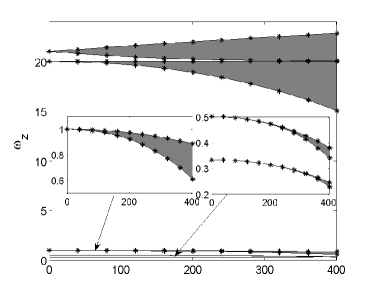
Figure 1: Plot of instability regions represented by the normalized frequency of the pump wave $\omega_{z}$ as a function of the normalized strength of the pump wave $E_{0}$. Parameters are chosen for the three-wave interaction in a typical hydrogen plasma with $\omega_{x}=1$, $\omega_{y}=20$, $\lambda_{x}=i\mu_{x}$ and $\lambda_{y}=i\mu_{y}$ with $\mu_{x}=-\mu_{y}m_{e}/m_{i}=-\mu_{y}/1836$ and $\mu_{y}=E_{0}.$ Shaded regions are unstable. Five instability bands are shown. There exit numerous narrow instability bands under the lowest band shown. The top three bands originate from $\omega_{z}=\omega_{x}+\omega_{y}$, $\omega_{z}=\omega_{y}$ and $\omega_{z}=\omega_{x}$ on the vertical axis. Only the uppermost instability band originates from the position satisfying condition (1) on the vertical axis.

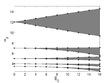
Figure 2: Plot of instability regions represented by the normalized frequency of the pump wave $\omega_{z}$ as a function of the normalized strength of the pump wave $E_{0}$. Parameters are chosen for the three-wave interaction with $\omega_{x}=5$, $\omega_{y}=7$, $\lambda_{x}/\lambda_{y}=-1$ and $\lambda_{y}=i\mu_{y}=iE_{0}$. Shaded regions are unstable. Five instability bands are shown. There exit numerous narrow instability bands under the lowest band shown. The top three bands originate from $\omega_{z}=\omega_{x}+\omega_{y}$, $\omega_{z}=\omega_{y}$ and $\omega_{z}=\omega_{x}$ on the vertical axis. Only the uppermost instability band originates from the position satisfying condition (1) on the vertical axis.

We start our investigation from Eqs. (2) and (3). Without losing generality, we focus on the three-wave interaction between a plasma wave, an ion-acoustic wave and an electromagnetic wave in an unmagnetized plasma Nishikawa (1968a, b). After normalizing independent variable $t$ and frequencies by the ion-acoustic frequency $\Omega_{k}$, we obtain the normalized ion-acoustic frequency $\omega_{x}=1$, the normalized plasma frequency $\omega_{y}=\omega_{e}/\Omega_{k}$ and the normalized frequency of the pump wave $\omega_{z}=\omega/\Omega_{k}$. The normalized coupling constants are $\lambda_{x}=i\mu_{x}$ and $\lambda_{y}=i\mu_{y}$ with $\mu_{x}=-\mu_{y}m_{e}/m_{i}$ and $\mu_{y}=E_{0}=ekE/m_{e}\Omega_{k}^{2}$. Here, $E$ is the amplitude of the pump wave and $E_{0}$ is the normalized amplitude, and $\mu_{x}$ or $\mu_{y}$ measures the strength of the pump wave. In this case, the pump wave is assumed to be spatially uniform (or with a long wavelength), and the plasma wave and the ion acoustic wave have opposite wave number $k$. In this normalization, the normalized variable $z(t)=2\cos(\omega_{z}t)$ describes the time-dependent pump wave. Also, we only consider the case without damping in the present study.

Equations (2) and (3) can be written as a 4-dimensional linear complex dynamical system

$$\mathbf{\dot{\mathbf{x}}}=A(t)\mathbf{x}\thinspace,$$ (5)

where

$$A(t) =\left(\begin{array}[]{cccc}0&0&-\omega_{x}^{2}&i\mu_{x}z(t)\\ 0&0&i\mu_{y}z(t)&-\omega_{y}^{2}\\ 1&0&0&0\\ 0&1&0&0\end{array}\right)\thinspace,$$ (10)

$$\mathbf{x} =\left(\begin{array}[]{cccc}dx/dt&dy/dt&x&y\end{array}\right)^{T}\thinspace.$$ (12)

A crucially important property of $A(t)$ is that it is a G-Hamiltonian matrix, meaning that it can be expressed as

$$A(t)=iG^{-1}S(t)\thinspace,$$ (13)

for a time-dependent Hermitian matrix $S(t)$ and an invertable constant Hermitian matrix $G$. This condition is equivalent to that of $A(t)$ satisfying

$$A(t)^{*}G+GA(t)=0\thinspace,$$ (14)

where $A(t)^{*}$ is the Hermitian conjugate of $A(t).$ The fact that $A(t)$ is a G-Hamiltonian matrix is the cornerstone of the physical mechanism of the three-wave instability. It brings out the Hamiltonian nature of the dynamics and thus determines the stability properties of system. By analyzing the expression of $A(t),$ we find that

$$G=\left(\begin{array}[]{cccc}0&0&-i\mu_{y}&0\\ 0&0&0&i\mu_{x}\\ i\mu_{y}&0&0&0\\ 0&-i\mu_{x}&0&0\end{array}\right)\thinspace$$ (15)

and

$$S(t)=\left(\begin{array}[]{cccc}-\mu_{y}&0&0&0\\ 0&\mu_{x}&0&0\\ 0&0&-\mu_{y}\omega_{x}^{2}&i\mu_{x}\mu_{y}z(t)\\ 0&0&-i\mu_{x}\mu_{y}z(t)&\mu_{x}\omega_{y}^{2}\end{array}\right).$$ (16)

Equation (5) is a special linear G-Hamiltonian system with the associated energy

$$H(\mathbf{x},t)=-\mathbf{x}^{*}S(t)\mathbf{x}\thinspace,$$ (17)

where $\mathbf{x}^{*}$ is the conjugate transpose of the vector $\mathbf{x}$. The definition of general G-Hamiltonian system has been given in Ref. Zhang et al. (2016). For $\mathbf{z}\in C^{n}$ and $\bar{\mathbf{z}}\in C^{n}$, the G-Hamiltonian system is a nature generation of complex Hamiltonian system, and it reads

$$\dot{\mathbf{z}} =\dfrac{1}{i}G^{-1}\dfrac{\partial H}{\partial\bar{\mathbf{z}}},$$ (18)

$$\dot{\bar{\mathbf{z}}} =-\dfrac{1}{i}\bar{G}^{-1}\dfrac{\partial H}{\partial\mathbf{z}},$$ (19)

where $G$ is a non-singular Hermitian matrix and $H(\mathbf{z},\bar{\mathbf{z}})$ satisfies the reality condition $H(\mathbf{z},\bar{\mathbf{z}})=\overline{H(\mathbf{z},\bar{\mathbf{z}})}$. Because of the reality condition, Eq.(18) and Eq.(19) are equivalent, and we only need to consider Eq.(18).

Solutions of Eq. (5) can be given as $\mathbf{x}(t)=X(t)\mathbf{x}(0)$ for a time evolution matrix, or solution map matrix, $X(t)$. Obviously, $X(t)$ satisfies

$$\dfrac{dX(t)}{dt}=A(t)X(t)\thinspace,$$ (20)

and the initial value $X(0)=I$. Since $A(t)$ is a G-Hamiltonian matrix, the corresponding time evolution matrix $X(t)$ is a G-unitary matrix, which means that it satisfies

$$X^{*}(t)GX(t)=G\thinspace.$$ (21)

This is because

$$\dfrac{d}{dt}\left[X(t)^{*}GX(t)\right]=\dfrac{d}{dt}X(t)^{*}GX(t)+X(t)^{*}G\dfrac{d}{d}X(t)$$ (22)

$$= X(t)^{*}A^{*}GX(t)+X^{*}GAX(t)=0\thinspace.$$

The eigenvalues of a G-unitary matrix is classified according to their Krein signatures, which is similar to the definition of the eigenvalues of a G-Hamiltonian matrix Zhang et al. (2016). It is associated with a bilinear product

$$\left\langle\mathbf{\psi},\phi\right\rangle=\phi^{*}G\psi\thinspace.$$ (23)

An $r-$fold eigenvalue $\rho$ ($|\rho|=1$) of a G-unitary matrix with its eigen-subspace $V_{\rho}$ is called the first kind of eigenvalue if $\left\langle\mathbf{y},\mathbf{y}\right\rangle>0$, for any $\mathbf{y}\neq 0$ in $V_{\rho}$, and the second kind of eigenvalue if $\left\langle\mathbf{y},\mathbf{y}\right\rangle<0$, for any $\mathbf{y}\neq 0$ in $V_{\rho}$. If there exists a $\mathbf{y}\in V_{\rho}$ such that $\left\langle\mathbf{y},\mathbf{y}\right\rangle=0$, then $\rho$ is called an eigenvalue of mixed kind Yakubovich and Starzhinskii (1958). The first kind and the second kind are also called definite, and the mixed kind is also called indefinite.

In the present case, $A(t)$ is periodic with period $T=2\pi/\omega_{z}$. So is the solution map matrix $X(t)$, and thus the dynamic properties of the system are given by the one-period map $X(T)$. Specifically, eigenvalues of $X(T)$ decide the stability property of the system. The relevant mathematical theory has been systematically developed by Krein, Gel’fand and Lidskii Krein (1950); Gel’fand and Lidskii (1955); Yakubovich and Starzhinskii (1958), which is listed as follows.

1. The eigenvalues of a G-unitary matrix are symmetric with respect to the unit circle.

2. The number of each kind of eigenvalue is determined by the Hermitian matrix $G$. Let p be the number of positive eigenvalues and q be the number of negative eigenvalues of the matrix $G$, then any G-unitary matrix has p eigenvalues of first kind and q eigenvalues of second kind (counting multiplicity).

3. (Krein-Gel’fand-Lidskii theorem) The G-Hamiltonian system is strongly stable if and only if all of the eigenvalues of the one-period map matrix $X(T)$ lie on the unit circle and are definite. Here, strongly stable means that the system is stable in an open neighborhood of the parameter space constrained by the G-Hamiltonian structure.

From the above mathematical results, we know that the eigenvalues of one-period evolution map $X(T)$ of a G-Hamiltonian system are symmetric about the unit circle. Moreover, because the eigenvalues of $G$ are $\pm\mu_{x},\pm\mu_{y}$, two of which are positive and the other two are negative, the G-unitary matrix $X(T)$ has two eigenvalues of the first kind and two eigenvalues of the second kind. When two eigenvalues of $X(T)$ with different Krein signatures collide on the unit circle, the G-Hamiltonian system Eq. (5) is destabilized. This process is called Krein collision. We now show its physical meaning. For a G-unitary matrix $X(T)$ whose eigenvalues are distinct and are all on the unit circle, it can be written as

$$X(T)=YDiag(e^{i\lambda_{1}},\cdots,e^{i\lambda_{4}})Y^{-1}\thinspace,$$ (24)

where $\lambda_{i}\in[0,2\pi]$ and $Diag(e^{i\lambda_{1}},\cdots,e^{i\lambda_{4}})$ is a diagonal matrix. We define

$$\ln X(T)=YDiag(i\lambda_{1},\cdots i\lambda_{4})Y^{-1}\thinspace.$$ (25)

Because $X(T)$ is a G-unitary matrix, we have

$$G^{-1}\left[\ln X(T)\right]^{*}G=\ln\left[G^{-1}X(T)^{*}G\right]=\ln\left[X(T)^{-1}\right]=-\ln X(T)\thinspace.$$ (26)

Thus $\ln X(T)/T$ is a G-Hamiltonian matrix and there is a Hermitian matrix $\hat{S}$, such that $\ln X(T)/T=iG^{-1}\hat{S}\thinspace.$ For an eigenvalue $\rho=\exp(i\lambda)$ of $X(T)$ on the unit circle with an eigenvector $\mathbf{y}$,

$$\mathbf{y}^{*}G\dfrac{\ln X(T)}{T}\mathbf{y} =i\mathbf{y}^{*}\hat{S}\mathbf{y}\thinspace.$$ (27)

Because of Eqs. (17) and (23), we obtain

$$<\mathbf{y},\mathbf{y}>=-\dfrac{T\hat{H}(\mathbf{y})}{\lambda}\thinspace.$$ (28)

Here, $T\hat{H}(y)$ is the action over one period and $\lambda$ is the argument of the eigenvalue $\rho$. It is clear that in a strongly stable system, the physical meaning of its Krein signature is the opposite sign of the action over one period. Therefore, the physical mechanism of the Krein-Gel’fand-Lidskii theorem is that the system becomes unstable when and only when a positive-action mode resonates with a negative-action mode.

We now demonstrate the aforementioned physical mechanism using numerically calculated examples for a typical hydrogen plasma. The normalized plasma frequency is chosen to be $\omega_{y}=20,$ and the normalized pump amplitude $\mu_{y}=E_{0}$ varies from $0$ to $400.$ For each $E_{0}$, the system is solved numerically for different values of $\omega_{z}$. The one-period evolution map $X(T)$ and its eigenvalues are calculated numerically. The instability regions in terms of frequency $\omega_{z}$ are plotted as functions of $E_{0}$ in Fig. 1. As discussed above, it shows clearly that resonant condition (1) cannot be used as the criteria for the onset of the three-wave instability in general. Instead, the instability thresholds are exactly the locations where a positive-action mode resonates a negative-action mode, which is shown in Figs. 3 and 4.

For the case of $E_{0}=320$, five instability intervals are shown in Fig. 1. First, let’s observe how the system behaves as $\omega_{z}$ traverses the uppermost instability threshold from the top. Shown in Fig. 3 are the eigenmodes numerically calculated. As expected, the eigenvalues of the matrix $X(T)$ are symmetric about unit circle and real axis. There are two sets, and each set contains two eigenvalues symmetric about real axis. When $\omega_{z}=24$, shown in Fig. 3(a), the eigenmodes are all on the unit circle and distinct, where $M_{1+}$ and $M_{2+}$ (marked by red) are eigenmodes with negative action, and $M_{1-}$ and $M_{2-}$ (marked by green) are eigenmodes with positive action. As $\omega_{z}$ decreases, the eigenmodes $M_{1+}$ and $M_{2+}$ rotate clockwise on the unit circle, meanwhile $M_{1-}$ and $M_{2-}$ rotate counterclockwise on the unit circle as shown in Fig. 3(b). Decreasing $\omega_{z}$ to $22.492$, we find in Fig. 3(c) that eigenmodes $M_{1+}$ and $M_{2-}$ collide on the unit circle, and simultaneously $M_{1-}$ and $M_{2+}$ collide on the unit circle. This marks the uppermost threshold of the instability. Then, when $\omega_{z}=22$, all eigenmodes move off the unit circle with $M_{1+}$ and $M_{1-}$ outside and $M_{2+}$ and $M_{2-}$ inside, as shown in Fig. 3(d). The system is now unstable, and $M_{1}$ and $M_{2}$ are the unstable modes.

Similarly, we can move $\omega_{z}$ upwards traversing the lower threshold of the second instability band. When $\omega_{z}=14$, shown in Fig. 4(a), the system is stable with four eigenmodes on the unit circle. As $\omega_{z}$ increases, $M_{1+}$ and $M_{1-}$ move towards each other as shown in Fig. 4(b), and they collide when $\omega_{z}=16.9854$, which marks the lowermost threshold of the instability in Fig. 4(c). Increasing $\omega_{z}$ to $17.5$, the $M_{1+}$ and $M_{1-}$ modes become unstable in Fig. 4(d). In the process, the $M_{2+}$ and $M_{2-}$ modes stay on the unit circle all the time, which is different from the case displayed in Fig. 3.

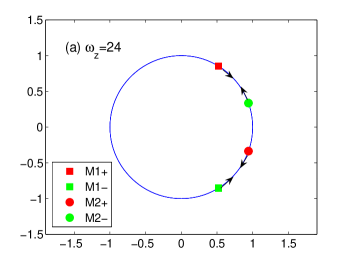
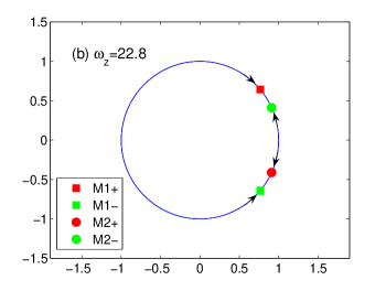
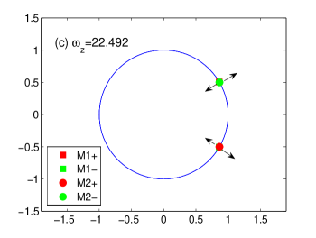
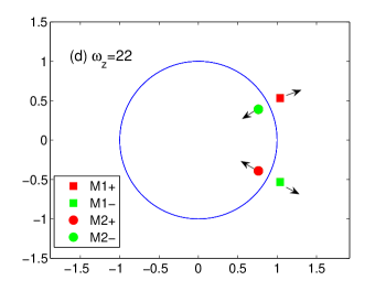
Figure 3: Krein collisions when varying $\omega_{z}$ downward at $\omega_{x}=1,\thinspace\omega_{y}=20,\thinspace\mu_{x}=-\mu_{y}/1836$, $\mu_{y}=E_{0}$ and $E_{0}=320$. Krein collision occurs at $\omega_{z}=22.492$.

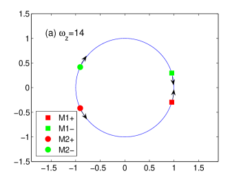
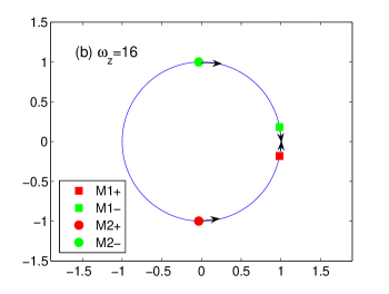
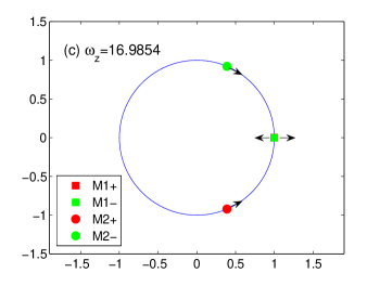
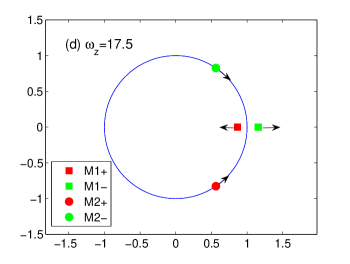
Figure 4: Krein collisions when varying $\omega_{z}$ upward at $\omega_{x}=1,\thinspace\omega_{y}=20,\thinspace\mu_{x}=-\mu_{y}/1836$, $\mu_{y}=E_{0}$ and $E_{0}=320$. Krein collision occurs at $\omega_{z}=16.9854$.

In conclusion, we have shown that for the dynamics of three-wave interaction, the familiar resonant condition $\omega_{z}\approx\omega_{x}+\omega_{y}$ is not the criteria for instability. The physical mechanism of the instability is the resonance between a positive-action mode with a negative-action mode, and this condition exactly marks the instability threshold. This mechanism is imposed by the topology and geometry of the spectral space determined by the complex G-Hamiltonian structure of the dynamics, which is a manifest of the infinite dimensional Hamiltonian structure in the wave-number space. Guided by this new theory, the additional instability bands for the three-wave interaction previously unknown are discovered. They originate from points on the vertical axis. We suspect that the mechanism of resonance between a positive- and negative-action modes may be crucial in predicting which point instability bands originate from. Study on this and other topics will be reported in the future.

This research is supported by the National Natural Science Foundation of China (NSFC-11505186, 11575185, 11575186), ITER-China Program (2015GB111003, 2014GB124005), the Geo-Algorithmic Plasma Simulator (GAPS) Project, and the U.S. Department of Energy (DE-AC02-09CH11466).

References

- Oraevskii and Sagdeev (1963) V. Oraevskii and R. Sagdeev, Sov. Phys.-Tech. Phys. 7, 955 (1963).
- Silin (1965) V. Silin, Sov. Phys. JETP 21, 1127 (1965).
- Nishikawa (1968a) K. Nishikawa, J. Phys. Soc. Jap. 24, 916 (1968a).
- Nishikawa (1968b) K. Nishikawa, J. Phys. Soc. Jap. 24, 1152 (1968b).
- Rosenbluth et al. (1973) M. Rosenbluth, R. White, and C. Liu, Phys. Rev. Lett. 31, 1190 (1973).
- Drake et al. (1974) J. F. Drake, P. K. Kaw, Y.-C. Lee, G. Schmid, C. S. Liu, and M. N. Rosenbluth, Phys. Fluids 17, 778 (1974).
- Kaup et al. (1979) D. Kaup, A. Reiman, and A. Bers, Rev. Mod. Phys. 51, 275 (1979).
- Jha and Srivastava (1975) S. S. Jha and S. Srivastava, Phys. Rev. A 11, 378 (1975).
- Malkin et al. (1999) V. Malkin, G. Shvets, and N. Fisch, Phys. Rev. Lett. 82, 4448 (1999).
- Dodin and Fisch (2002) I. Y. Dodin and N. Fisch, Phys. Rev. Lett. 88, 165001 (2002).
- Hasegawa (2012) A. Hasegawa, Plasma instabilities and nonlinear effects, Vol. 8 (Springer Science & Business Media, 2012).
- Kaw (2017) P. Kaw, Rev. Mod. Plasma Phys. 1, 1 (2017).
- Ping et al. (2004) Y. Ping, W. Cheng, S. Suckewer, D. S. Clark, and N. J. Fisch, Phys. Rev. Lett. 92, 175007 (2004).
- Shi et al. (2017) Y. Shi, H. Qin, and N. J. Fisch, Phys. Rev. E 95, 023211 (2017).
- Shen and Bloembergen (1965) Y. R. Shen and N. Bloembergen, Phys. Rev. 137, A1787 (1965).
- Bloembergen and Shen (1964) N. Bloembergen and Y. Shen, Phys. Rev. Lett. 12, 504 (1964).
- Blow and Wood (1989) K. J. Blow and D. Wood, IEEE J. Quantum Electron. 25, 2665 (1989).
- Singh et al. (2007) S. P. Singh, R. Gangwar, and N. Singh, Prog. Electromagn. Res. 74, 379 (2007).
- Leo et al. (2016) F. Leo, T. Hansson, I. Ricciardi, M. De Rosa, S. Coen, S. Wabnitz, and M. Erkintalo, Phys. Rev. Lett. 116, 033901 (2016).
- Picozzi and Haelterman (2001) A. Picozzi and M. Haelterman, Phys. Rev. Lett. 86, 2010 (2001).
- Buryak et al. (2002) A. V. Buryak, P. Di Trapani, D. V. Skryabin, and S. Trillo, Phys. Rep. 370, 63 (2002).
- Chen et al. (2015a) S. Chen, F. Baronio, J. Soto-Crespo, P. Grelu, M. Conforti, and S. Wabnitz, Phys. Rev. A 92, 033847 (2015a).
- Chen et al. (2015b) S. Chen, J. M. Soto-Crespo, and P. Grelu, Opt. Express 23, 349 (2015b).
- Craik (1988) A. D. Craik, Wave interactions and fluid flows (Cambridge University Press, 1988).
- Aubourg and Mordant (2015) Q. Aubourg and N. Mordant, Phys. Rev. Lett. 114, 144501 (2015).
- Haudin et al. (2016) F. Haudin, A. Cazaubiel, L. Deike, T. Jamin, E. Falcon, and M. Berhanu, Phys. Rev. E 93, 043110 (2016).
- Bonnefoy et al. (2016) F. Bonnefoy, F. Haudin, G. Michel, B. Semin, T. Humbert, S. Aumaître, M. Berhanu, and E. Falcon, J. Fluid Mech. 805 (2016).
- Magnus and Winkler (1976) W. Magnus and S. Winkler, Hill’s equation (Dover, 1976).
- Brown et al. (2013) B. Brown, M. Eastham, and K. Schmidt, Periodic Differential Operators (Springer Basel, 2013) pp. 94–105.
- Krein (1950) M. Krein, Doklady Akad. Nauk. SSSR N.S. 73, 445 (1950).
- Gel’fand and Lidskii (1955) I. M. Gel’fand and V. B. Lidskii, Uspekhi Mat. Nauk 10, 3 (1955).
- Yakubovich and Starzhinskii (1958) V. Yakubovich and V. Starzhinskii, Linear Differential Equations with Periodic Coefficients, Vol. I (1958).
- Zhang et al. (2016) R. Zhang, H. Qin, R. C. Davidson, J. Liu, and J. Xiao, Phys. Plasmas 23, 072111 (2016).
- Kirillov (2017) O. N. Kirillov, Proc. R. Soc. A, Proc. R. Soc. A 473, 20170344 (2017).
- Crabtree et al. (2017) C. Crabtree, G. Ganguli, and E. Tejero, Phys. Plasmas 24, 056501 (2017).