Detecting topological properties of Markov compacta with combinatorial properties of their diagrams

Abstract.

We develop a formalism that allows us to describe Markov compacta with finite sets of diagrams that are building blocks of the entire sequence. This encodes complex, continuous spaces with discrete collections of combinatorial objects. We show that topological properties of the limit (such as $k$-connectedness, local $k$-connectedness or the disjoint arcs property) may be detected by looking at combinatorial properties of the diagrams.

Markov compacta were introduced by M. Gromov and were motivated by some examples in geometric group theory. In particular, boundaries at infinity of hyperbolic groups belong to this class.

1. Introduction

Consider the following inverse sequence.

The $n$-th space $K_{n}$ of this sequence is a discrete space with $2^{n-1}$ elements and each bonding map $p_{n}$ has $2$-element fibers. The inverse limit of this sequence is homeomorphic to the Cantor set. Observe that the whole sequence can be recreated using a single diagram

which can be considered a “building block" of the sequence. Similarily, the classical inverse sequence used to define a solenoid

can be encoded using the following two “building blocks” and colors (represented by solid and dotted lines) that describe the “gluing” process.

Both the Cantor set and the solenoid are examples of Markov compacta.The class of Markov compacta was introduced by M. Gromov and was motivated by some examples in geometric group theory. In particular, boundaries at infinity of hyperbolic groups belong to this class [7].

In the present paper we develop a formalism that allows us to encode Markov compacta using finite sets of diagrams and gluing rules similar to the diagrams depicted above. This allows us to encode complex, continuous topological spaces using a discrete collection of finite complexes. We show that some topological properties of the limit space (such as connectedness, local connectedness or the disjoint arcs property) can be detected by the combinatorial properties of the diagrams. In particular, we give examples of Markov spaces that are homeomorphic to Menger cubes and Nöbeling spaces. Detecting topological properties that characterize these spaces is important for applications. For example, by theorems of Hensel-Przytycki [6] and Gabai [5] the boundary at infinity of a curve complex (which is a hyperbolic graph) of a sphere punctured $n+5$ times is homeomorphic to the $n$-dimensional Nöbeling space. Moreover, Dymara and Osajda [3] have shown that the boundary of a right-angled hyperbolic building is a universal Menger space. The characterization of boundaries of curve complexes of higher genus surfaces with punctures is open.

We focus on the one-dimensional case, where all polyhedra in the sequence are graphs. This case covers a wide class of interesting examples.

This paper opens a new avenue of research: to determine which topological properties of Markov compacta can be detected by combinatorial properties of its diagram.

2. Markov Spaces

Definition 2.1.

Let $K$ be a simplicial complex. Let $\tau(K)$ be the triangulation of $K$. We let $\beta K$ denote the barycentric subdivision of $K$ (i.e., the same metric space but with finer triangulation $\tau(\beta K)$). A coloring of $K$ is a map from $\tau(K)$ to $\mathbb{N}$. A colored complex is a simplicial complex with fixed coloring. We let $c(K)\colon K\to\mathbb{N}$ denote the coloring of a colored complex $K$. A colored embedding is a simplicial embedding $i\colon K\to L$ of colored complexes $K$ and $L$ such that $c(K)=c(L)\circ i$.

Definition 2.2.

Let $K$ and $L$ be simplicial complexes and let $p\colon K\to L$. We say that $p$ is quasi-simplicial if it is a simplicial map into $\beta L$.

Definition 2.3.

A production $P$ is a simplicial or quasi-simplicial map $P\colon K\to L$ from a colored complex $P$ into a colored complex $K$. We call $K$ the top complex of the production and denote it by $t(P)$. We call $L$ the bottom complex of the production and denote it by $b(P)$.

Definition 2.4.

Let $S$ and $T$ be productions. A gluing $G$ is a pair of maps $(G_{t}\colon t(S)\to t(T),G_{b}\colon b(S)\to b(T))$ that are colored embeddings such that the following diagram is commutative

Definition 2.5.

A Markov diagram $\mathcal{D}$ is a triple $\mathcal{D}=(S,\mathcal{P},\mathcal{G})$, where $S$ is a simplicial complex that we call the starting complex of $\mathcal{D}$, $\mathcal{P}$ is a set of productions that we call the production set of $\mathcal{D}$ and $\mathcal{G}$ is a set of gluings that we call the set of gluing rules of $\mathcal{D}$.

Definition 2.6.

Let $\mathcal{D}=(S,\mathcal{P},\mathcal{G})$ be a Markov diagram. Let $\Gamma=(V,E)$ be a directed graph. Let $P\colon V\to\mathcal{P}$ be a labelling of vertices of $\Gamma$ by productions of $\mathcal{D}$. Let $G\colon E\to\mathcal{G}$ be a labelling of edges of $\Gamma$ by gluings of $\mathcal{D}$. If for each directed edge $e=(u,v)$ of $\Gamma$ the following diagram is commutative

then we say that $\Gamma$ is an assembly graph for $\mathcal{D}$.

Definition 2.7.

Let $K,L$ be colored complexes. Let $f\colon K\to L$ be a simplicial or a quasi-simplicial map. Let $\mathcal{D}=(S,\mathcal{P},\mathcal{G})$ be a Markov diagram. Let $\Gamma=(V,E)$ be an assembly graph for $\mathcal{D}$ with labelling $P\colon V\to\mathcal{P}$ of vertices and labelling $G\colon E\to\mathcal{G}$ of edges.

Let $\mathcal{T}=\{f_{v}\colon t(P(v))\to K\}_{v\in V}$ and $\mathcal{B}=\{g_{v}\colon b(P(v))\to L\}_{v\in V}$ be collections of colored embeddings. Assume that for each edge $e=(u,v)\in V$ the following diagram is commutative

Assume that $\{\operatorname{im}f_{v}\}_{v\in V}$ is a cover of $K$ that is closed under intersection and $\{\operatorname{im}g_{v}\}_{v\in V}$ is a cover of $L$ that is closed under intersection.

Then we say that $(\mathcal{T},\mathcal{B})$ is a chart for $f$. We call $\mathcal{T}$ the top chart and $\mathcal{B}$ the bottom chart for $f$. The structure $(\Gamma,\mathcal{T},\mathcal{B})$ satisfying the above conditions is called a decomposition of $f$ with respect to $\mathcal{D}$.

Definition 2.8.

Let $\mathcal{D}$ be a Markov diagram. A Markov sequence is an inverse sequence

$$K_{1}\xleftarrow{p_{1}}K_{2}\xleftarrow{p_{2}}K_{3}\xleftarrow{p_{3}}\cdots$$

along with a decompositions of all bonding maps $p_{i}$ over $\mathcal{D}$. The limit of the sequence

$$\lim_{\longleftarrow}\left(K_{1}\xleftarrow{p_{1}}K_{2}\xleftarrow{p_{2}}K_{3}\xleftarrow{p_{3}}\cdots\right)$$

is called a Markov space. If complexes $K_{i}$ are $1$-dimensional, then we call the limit a Markov curve.

2.1. The $1$–$8$ sequence

All graphs in this section are mono-colored. The $1$–$8$ sequence is named after a single edge production $P_{8}$ it contains.

The production map $P_{8}$ is the vertical quasi-simplicial projection from the top $8$-shaped graph $t(P_{8})$ onto the single-edge graph $b(P_{8})$ on the bottom. The production set is completed by a single vertex production $P_{1}$.

The production map $P_{1}$ projects horizontally the right edge graph $t(P_{1})$ onto a single vertex graph $b(P_{1})$ on the left. We let $\mathcal{P}=\{P_{1},P_{8}\}$ be the production set of the $1$–$8$ sequence. There are two gluing rules in the $1$–$8$ sequence, the left gluing $G_{l}$ and the right gluing $G_{r}$.

We let $\mathcal{G}=\{G_{l},G_{r}\}$ be the set of gluing rules of the $1$–$8$ sequence. The starting graph is a single edge graph

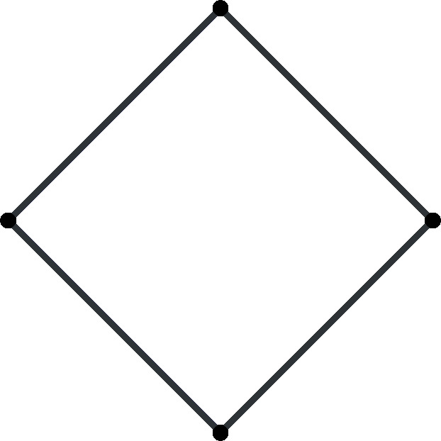
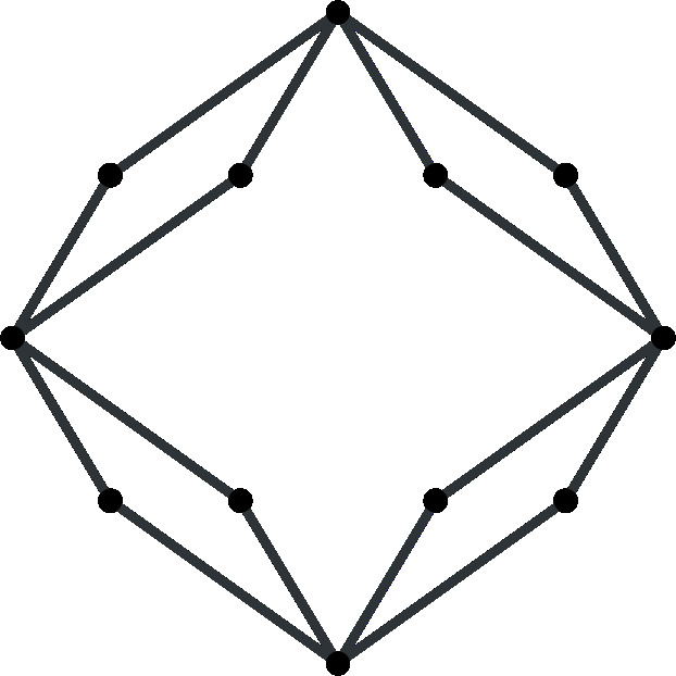
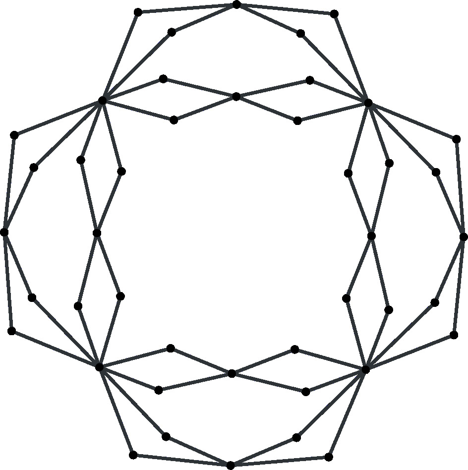
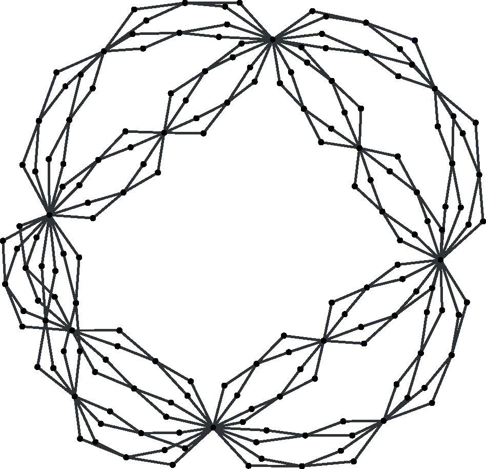
The triple $\mathcal{D}=(S,\mathcal{P},\mathcal{G})$ is a Markov diagram, which we call the $1$–$8$ diagram. Below are first six elements of a Markov sequence that corresponds to this diagram.

	$\leftarrow$		$\leftarrow$		$\leftarrow$
	$\leftarrow$		$\leftarrow$		$\leftarrow$		$\leftarrow$	$\cdots$

We will show how the first bonding map $p_{1}$ decomposes over $\mathcal{D}$. We take an assembly graph $\Gamma_{1}$:

The vertices of $\Gamma_{1}$ are labeled with productions $P_{1}$ and $P_{8}$, edges are labeled with gluings $G_{l}$ and $G_{r}$. This yields a commutative diagram of upper and lower charts, which is a decomposition of $p_{1}$ over $\Gamma_{1}$.

The other bonding maps can be decomposed in a similar way. We will show in the later sections that the limit of the $1$–$8$ sequence is homeomorphic to the universal Menger curve $M^{3}_{1}$.

Definition 2.9.

We say that a Markov sequence is an elementary Markov sequence if the bottom graphs of its productions are either single vertex graphs or single edge graphs.

For a simplicial complex, the underlying polyhedron has two topologies, the Whitehead (weak) topology and the metric topology. The weak topology is metrizable if and only if the complex is locally finite and it coincides with the metric topology in this case. Since we work in the metric category with complexes that are not locally finite, we always assume the metric topology on simplicial complexes.

Definition 2.10.

Let $K$ be simplicial complex. We let $\tau(K)$ denote the triangulation of $K$ (the set of simplices of $K$). We let $V(K)$ denote the vertex set of $K$. We let $\beta K$ denote the barycentric subdivision of $K$ (i.e., the same metric space but with finer triangulation $\tau(\beta K)$).

Definition 2.11.

Let $K$ be a simplicial complex. Let $\kappa\in(0,\infty)$. We define a geodesic metric of scale $\kappa$ on $K$ in the following way. On each $\delta\in\tau(K)$ we take a Euclidean metric with edge length $\kappa$. We extend this on $K$ to the unique geodesic metric.

Lemma 2.12.

The metric defined in Definition 2.11 induces the metric topology.

3. Examples

3.1. Cantor set

A Markov diagram that generates a Markov sequence described in the Introduction that generates the Cantor set contains a single point as a starting graph, a single production

that maps a two-vertex graph onto a single-vertex graph with no gluing rules. There exists a unique inverse sequence corresponding to this diagram.

$\leftarrow$

$\leftarrow$

$\leftarrow$

$\leftarrow$

$\leftarrow$

$\leftarrow\ \ \ \cdots$

The threads in this inverse limit can be mapped homeomorphically onto the set of binary sequences $\{0,1\}^{\infty}$ with the product topology, which is homeomorphic to the Cantor set.

3.2. The suspension of the Cantor set

If we “suspend" the diagram for the Cantor set we will get a suspension of the Cantor set in the limit. The only non single vertex production is production $P$.

Here we use different color to mark end points of the suspension. We define a single vertex production

corresponding to the horizontal top and bottom fibers of $P$. We define gluings that glue these single vertex productions into the corresponding fibers of $P$. We will usually omit these when presenting Markov diagrams. Note that the Markov diagram does not contain a production for the middle hollow vertex of $P$; it is not needed since gluings are performed only along the top and bottom vertices.

We define the starting space . The following sequence of spaces is produced.

Observe that the limit space is connected, but not locally connected. The horizontal cross sections are homeomorphic to the Cantor set, with the exception of the end points.

3.3. A diamond sequence

A diamond sequence is an elementary Markov sequence that starts with a single edge and contains a trivial vertex production along with a single edge production.

There are two gluing rules on fibers of the edge production.

$\leftarrow$

$\leftarrow$

$\leftarrow$

$\leftarrow$

$\leftarrow$

$\cdots$

Figure 1. A diamond sequence. The layout of the last two graphs was generated using SFDP spring-block algorithm, hence the irregularities.

The limit of this sequence is a $1$-dimensional connected and locally connected compactum that we call a diamond curve.

3.4. Join of two Cantor sets

An elementary Markov sequence that starts with a single edge and contains a double vertex production along with a single edge production depicted in the following diagram.

The first six graphs from the sequence are shown below. The inverse limit is homeomorphic to a join of two Cantor sets.

	$\leftarrow$		$\leftarrow$		$\leftarrow$
	$\leftarrow$		$\leftarrow$		$\leftarrow$		$\leftarrow$	$\cdots$

3.5. Solenoid

So far in our examples we only used mono-colored graphs. We shall use colored graphs to describe productions that describe the solenoid. We have two edge productions.

The inverse sequence corresponding to this diagram is

The limit space is the solenoid [4], directly from the definition.

4. Topological properties

4.1. $k$-Connectedness and local $k$-connectedness

We prove the following sufficient condition for $k$-connectedness and local $k$-connectedness of a Markov space.

Theorem 4.1.

Let $X$ be a Markov space that is the inverse limit of a sequence

$$K_{1}\xleftarrow{p_{1}}K_{2}\xleftarrow{p_{2}}K_{3}\xleftarrow{p_{3}}\cdots.$$

Assume that the sequence decomposes over a Markov diagram $\mathcal{D}$. If for each production $P$ in $\mathcal{D}$, $P$ is quasi-simplicial, the top complex $t(P)$ is $k$-connected for each $k<n$, and the starting space is $k$-connected for each $k<n$, then $X$ is $k$-connected and locally $k$-connected for each $k<n$.

Proof.

Fix $k<n$ and let $\varphi\colon S^{k}\to X$. Let $\mathcal{D}_{i}$ be a decomposition of the space $K_{i}$ in the sequence. We will show that the inverse sequence $K_{1}\xleftarrow{p_{1}}K_{2}\xleftarrow{p_{2}}\cdots$ along with the sequence $\mathcal{D}_{i}$ of covers satisfies conditions of [1, Lemma 4.3]. Then if $\varPhi\colon B^{k+1}\to K_{1}$ is a null-homotopy of $\pi_{1}\circ\varphi$ (which exists because the starting space $K_{1}$ is $k$-connected), by [1, Lemma 4.3] $\varPhi$ can be lifted to a map into $X$ that extends $\varphi$, which implies that $X$ is $k$-connected.

To verify that conditions of [1, Lemma 4.3] are satisfied we need to verify that the sequence $\mathcal{D}_{i}$ of covers satisfies conditions of [1, Definition 4.2].

By Lemma 2.12, each $K_{i}$ is complete metric space (condition (A)) and each bonding map is $1$-Lipschitz (condition (B)). By the definition, each decomposition is closed, locally finite cover (condition (C)). By the assumption on top graphs, the pull-back $p_{i}^{-1}(\mathcal{D}_{i})$ is $k$-connected and locally $k$-connected for each $k<n$. By [1, Theorem 3.1], it is an $AE(n)$-cover (condition (D)). Again, by Lemma 2.12, $\sum_{i=1}^{\infty}\operatorname{mesh}\mathcal{D}_{i}<\infty$ (condition (E)). We are done.

To prove that $X$ is locally connected consider $x\in X$ and an open neighborhood $U$ of $x$. Let $i$ such that $B(\operatorname{st}_{\mathcal{D}_{i}}\pi_{i}(x),\sum_{k\geq i}\operatorname{mesh}\mathcal{D}_{i})\subset U$. Let $V=\pi_{i}^{-1}(\operatorname{st}\pi_{i}(x))$. Observe that $\pi_{i}(V)$ is $k$-connected. If we repeat the above argument for a sequence $K_{i}\xleftarrow{p_{i}}K_{i+1}\xleftarrow{p_{i+1}}\cdots$, we get that any map $\varphi\colon S^{k}\to V$ is null-homotopic in $U$, hence $X$ is locally $k$-connected. ∎

Remark 4.2.

The combinatorial property that implies connectedness conditions stated in Theorem 4.1 is “color-blind", i.e. it does not use colorings of the productions in any way.

Remark 4.3.

The condition that production maps are quasi-simplicial in statement of Theorem 4.1 is necessary. In the suspension of the Cantor set example, the top graphs of the productions are connected, yet the limit is not locally connected. In the diamond sequence example the maps are quasi-simplicial and the diamond space is indeed locally connected.

4.2. Disjoint arcs property

We prove a sufficient condition for the disjoint arcs property of a compact Markov curve.

Definition 4.4.

A compact space $X$ has disjoint the arcs property if for each map $f\colon[0,1]\times\{0,1\}\to X$ and each $\varepsilon>0$ there exists a map $f^{\prime}\colon[0,1]\times\{0,1\}\to X$ that is $\epsilon$-close to $f$ and such that $f^{\prime}([0,1]\times\{0\})\cap f^{\prime}([0,1]\times\{1\})=\emptyset$.

Theorem 4.5.

Let $X$ be a Markov space that is the inverse limit of a sequence

$$K_{1}\xleftarrow{p_{1}}K_{2}\xleftarrow{p_{2}}K_{3}\xleftarrow{p_{3}}\cdots.$$

Assume that for each $i$, $K_{i}$ is a finite graph. Assume that the sequence decomposes over an elementary Markov diagram $\mathcal{D}$ such that the vertex productions are isomorphic to and the edge productions have a connected and biconnected top graph. Then $X$ has the disjoint arcs property.

Proof.

As a first step we shall prove that for each $i$ there exist a pair of embeddings $f_{i},g_{i}\colon K_{i}\to K_{i+1}$ such that $\operatorname{im}f_{i}\cap\operatorname{im}g_{i}=\emptyset$ and $p_{i}\circ f_{i}=p_{i}\circ g_{i}=\operatorname{id}_{K_{i}}$.

For each vertex production, mark the two vertices of the top single-edge graph with the letters $A$ and $B$. Since the top graphs of the edge productions are biconnected, for each gluing of the vertex productions onto the end points of the edge production we may select disjoint paths in the top graph connecting vertices marked with $A$ and vertices marked with $B$. We construct $f_{i}$ to map the vertices of $K_{i}$ onto the corresponding vertices of $K_{i+1}$ marked with $A$ and such that it maps edges onto the selected paths. We perform a similar construction for $g_{i}$.

Take $\varepsilon>0$. Fix $i$ such that the scale of $K_{i}$ is smaller than $\frac{1}{3}\varepsilon$. Let $f\colon[0,1]\times\{0,1\}\to X$. Observe that $f_{i}\circ\pi_{i}\circ f$ and $g_{i}\circ\pi_{i}\circ f$ are disjoint. By [1, Lemma 4.3] we may lift these maps to $X$ in such a way that these lifts will be $\varepsilon$-close. Since their projections onto $K_{i}$ are disjoint, the maps are disjoint. We are done. ∎

4.3. Application to the $1$–$8$ sequence

We are now ready to prove that the inverse limit of the $1$–$8$ sequence defined in Subsection 2.1 is homeomorphic to the Menger curve $M^{3}_{1}$.

Theorem 4.6.

The inverse limit of an elementary Markov sequence that decomposes over production

with a connected finite starting graph is homeomorphic to the Menger curve $M^{3}_{1}$.

Proof.

Denote the limit space by $X$. Observe that the production maps of the Markov diagram are quasi-simplicial, have connected top graphs, and the starting graph is connected. By Theorem 4.1, $X$ is connected and locally connected. Since each space in the sequence is a finite graph, the inverse limit is compact and at most $1$-dimensional. Since $X$ contains at least two points and is path-connected, it is at least $1$-dimensional. By Theorem 4.5, $X$ has the disjoint arcs property.

We have shown that $X$ is compact, $1$-dimensional, connected, locally connected, and has disjoint arcs property. By Bestvina’s characterization theorem [2], $X$ is homeomorphic to $M^{3}_{1}$. ∎

References

- [1] G. Bell and A. Nagórko. Local -connectedness of inverse limits of polyhedra. preprint, 2017.
- [2] M. Bestvina. Characterizing -dimensional universal Menger compacta. Mem. Amer. Math. Soc., 71(380):vi+110, 1988.
- [3] J. Dymara and D. Osajda. Boundaries of right-angled hyperbolic buildings. Fund. Math., 197:123–165, 2007.
- [4] R. Engelking and K. Sieklucki. Topology: a geometric approach, volume 4 of Sigma Series in Pure Mathematics. Heldermann Verlag, Berlin, 1992.
- [5] D. Gabai. On the topology of ending lamination space. ArXiv e-prints, May 2011.
- [6] S. Hensel and P. Przytycki. The ending lamination space of the five-punctured sphere is the Nöbeling curve. J. Lond. Math. Soc. (2), 84(1):103–119, 2011.
- [7] D. Pawlik. Gromov boundaries as Markov compacta. ArXiv e-prints, Mar. 2015.