Examination of artifact in vector magnetic field SDO/HMI measurements

1 Introduction

S1

Satellite vector magnetic data from the SDO/HMI spacecraft represent a significant breakthrough in solar magnetography. Spatial resolution, quality of full disk vector magnetograms, regularity and high duty cadence of observations have no analogue neither in Earth, nor in satellite measurements. Invaluable is the contribution that can be made in the nearest future by the ever-growing time series of continuous observations for space weather predictions and fundamental research of magnetic nature of the solar activity. In particular, we can expect a considerable improvement in reliability of prediction of the solar wind parameters and IMF polarity of circumterrestrial space owing to the possibility of using the new vector synoptic maps (Gosain et al., 2013). To reconstruct the current global 3D structure of the filed in potential approximation and further modeling of the solar wind, longitudinal field synoptic maps were used in the past (Harvey et al., 1980). The advantage of new vector synoptic maps is brought about by two aspects. First, employing vector measurements enables us to extrapolate the field for the boundary field radial component (Neumann problem). Physically, such definition of the extrapolation problem is better substantiated comparing with extrapolation for longitudinal component, because the actual measurements are taken at the level where both potential approximation and even more general force-free approximation are sure not applicable . In these circumstances, different boundary value problems must inevitably lead to different results of extrapolation; these results, among the rest will give different components of a radial field at the boundary. Second, we construct Br synoptic map as a map for scalar value (unlike $B_{LOS}$ maps). This is an important point, since reconstruction of synoptic map for a non-scalar value is not quite correct.

For any large project that puts some new physical data into common use, it is strategically important remove, if possible, any significant artificial or natural errors, should such be present and can be identified. This is desirable to be done either before employing this information, or in the very beginning. Our work deals with exactly such kind of problem for the new SDO/HMI data. Herein we ascertain the fact of existence of a significant systematic error in the data submitted. We identify clearly this error from the analysis of the measurements data of knot magnetic fields that concentrate in the convection cell grid nodes of the quiet Sun. The observed magnetic knots result from the surrounding plasma raking up magnetic pipes by horizontal motions; this leads to magnetic flux concentration and subsequent radialization of the field. The compactness property of knot fields and significant excess of their magnitude relative to background values ($>500\ G$) enables us to select them using a sufficiently simple algorithm. The knot field inherent radiality is used as the main criterion for testing the magnetic field measurement data. We show (section 2) that the same systematic deviation (up to $20$ degrees) of the knot field from the radial direction toward the limb is revealed in all SDO/HMI vector magnetograms. This deviation depends on the distance to the disk center. Since observation result must not depend on observer position, we conclude that the revealed dependence can only have an artificial cause; this cause is likely unrecoverable in modern technologies for receiving and processing Stokes parameters used to obtain final values of vector magnetic field. In Section 3 we propose the idea of correcting the initial original vector magnetograms, based on the assumption that the systematic deviation from the radiality should be absent, and its presence is consequence of the presence of an error in the data of the angle of the field inclination relative to the line of sight. The manifestations of this error in the knots fields lead to the observed dependence of the deviation from the radiality on the position of the measurement point on the disk. We show that our correction almost eliminates effects of unnatural behavior of knot fields. Unlike the original magnetograms, the corrected ones do not contradict the results of the virial theorem for a nonlinear field (Livshits et al., 2015)(Livshits et al.2015)-”virial” energy is positive (first of all), it exceeds the energy of the reference potential field.

2 Identification and Analysis of Knot Fields

S2

2.1 Selection and Geometric Interpretation of Knot Magnetic Fields

S2.1 Our examination relies on the natural assumption about radiality of isolated small-scale magnetic structures of large magnitudes. Most of such structures correspond to the knots that concentrate in the convection cell grid nodes of the quiet Sun. Selection of the structures of our interest and determination of their physical properties from the magnetograms can be described with the Selection Algorithm (SA) as follows:
– using the IDL procedure ”LABEL_REGION”, we choose the full set of isolated regions with the $\left|{\bf B}\right|>300\ G$ values;
– from the obtained set, we select only the $A_{n}$ regions with pixel number not more than $35$ and $max\left|{\bf B}(A_{n})\right|>500\ G$;
– for each $A_{n}$ we find pixel $\left(i^{n}_{max},j^{n}_{max}\right):\left|{\bf B}\left(i^{n}_{max},j^{n}_{max}\right)\right|=max|{\bf B}(A_{n})|$;
– to each $A_{n}$ we assign value of magnetic field ${\bf B}^{n}={\bf B}(i_{max}^{n},j_{max}^{n})$ and radius-vector $r^{n}=r(i_{max}^{n},j_{max}^{n})$.
The values of $B^{n}$ and $r^{n}$ are used for further analysis. For simplicity, we will further omit index.

Figure kfig1 shows a typical example of defining location of the centers of knot regions (highlighted with red crosses). The detected knot regions are distributed evenly enough throughout the entire regions of the quiet Sun; they have slight higher concentration near active regions (green).

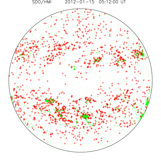
Figure 1.: SDO/HMI 2012-01-1505:12:00UT. Typical distribution of magnetic knots over the solar disk: $|{\bf B}|>300\ G$ –green points, knots – red crosses.kfig1

To assess the degree of radiality of the field of the knot regions, we will use the following three values (knot parameters $B_{r}^{LOS}/|{\bf B}|,\alpha,\beta)$:
– $B_{r}^{LOS}/|{\bf B}|$ is

$$\ilabel{keq1}B_{r}^{LOS}/|{\bf B}|=\frac{B_{LOS}}{\cos\mu}/|{\bf B}|,$$ (1)

where $B_{LOS}=B_{z}$ is projection of vector B along the line of sight, $\mu$ is the angle between the line of sight and the radius-vector of the knot location on the disk ($B_{r}^{LOS}=|B_{r}|=|{\bf B}|$ when the field is exactly radial);
– $\alpha$ is the angle between the observation point radius-vector and magnetic field component in meridional plane that is determined by the observation point radius-vector and the line of sight $z$-axis ($\alpha>0$ toward the limb, $\alpha=0$ when the field is exactly radial);
– $\beta$ is the angle between the vector of field line (always believed to be directed away from the Sun) and meridional plane ($\beta=0$ when the field is exactly radial). Figure kfig2 shows geometry of the angles $\alpha$ and $\beta$.

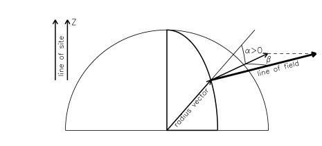
Figure 2.: Angular characteristics of the deviation from the magnetic field vector radiality.kfig2

It is important to note that to derive the value $B_{r}^{LOS}/|{\bf B}|$ we don’t need the information about the azimuthal field direction. Only, we need to eliminate $\pi$-uncertainty of the  $\phi$ azimuth to obtain the angular knot parameters $\alpha$ and $\beta$ . In this paper, we used the method described in (ambig) to eliminate the $\pi$-uncertainty.

2.2 Distribution of HMI Knot Parameters Over the Disk

S2.2 In our paper we examined the knot parameters characterizing deviation of the knot field from radiality for quite a large set of randomly time-selected SDO/HMI magnetograms ($=30$) for 2012-2014. In all magnetograms, parameters $B_{r}^{LOS}/|{\bf B}|$, $\alpha$ and $\beta$ demonstrate factually identical behavior on the solar disk (see Figure kfig1) From Figure kfig3, it follows that only the $\beta$ parameter demonstrates the expected – in case there are no data artifacts – statistic behavior with zero-mean.

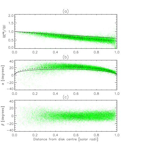
Figure 3.: Dependence of knots parameters on the distance to the solar disk center: (a) - $|B_{r}^{LOS}|/|{\bf B}|$; (b) - $\alpha$, (c) - $\beta$; green - for the full set of magnetograms, black - points of one magnetogram SDO / HMI 2012-01-15 05:12:00 UT.kfig3

The other parameters $|B_{r}^{LOS}|/|{\bf B}|$, $\alpha$ show a clear dependence of their averages on the distance to the solar disk center. On the one hand, non-zero $|B_{r}^{LOS}|/|{\bf B}|$, $\alpha$ contradict the hypothesis of radiality of the knots fields; on the other hand, their dependence on the distance to the center of the solar disk indicates the presence of an error of artificial origin in the data. Indeed, even if we exclude the property of radiality in the selected magnetic elements, in this case there should be, in principle, no statistical connection between knots parameters and the distance to the center of the solar disk. The same magnetic elements can not give different values of the field, depending on their visible position on the solar disk. It is also clear that the error we reveal can not be a consequence of the subsequent processing of the initial magnetograms associated with the method of solving the π-uncertainty problem of the transverse magnetic component of the measurements. In the case of an error generated only by solving the π-uncertainty problem, we would not observe any relationship with the distance of $|B_{r}^{LOS}|/|{\bf B}|$, which does not have $\pi$-uncertainty. Note the maximum deviation of the angle α is of the order of $20$ degrees at medium distances and the decrease of the $|B_{r}^{LOS}|/|{\bf B}|$ - ratio near the limb almost is $2$ times; that indicate the essentiality of the artificial error magnitudes.

Let us take notice of the apparent simplicity of relationship between the $|B_{r}^{LOS}|/|{\bf B}|$ value and the distance; in Figure kfig3 (a), this relationship is visually perceived as close to linear. Let us write it down in the form

$$\ilabel{keq2}B_{r}^{LOS}/|{\bf B}|=1-kr_{\perp},$$ (2)

where $r_{\perp}$ is the distance to the disk center in solar radii. On the full set of magnetograms, we obtained a fitting value of the Formula (keq2) linear coefficient, this fitting value equals

$$\ilabel{keq3}k=k_{fit}=0.565,$$ (3)

Figure kfig3 (a) shows the relevant dependence as a dashed line (we will comment later on the solid line in Figure kfig3 (a) and the lines in Figure kfig3 (b)).

Note that our results, shown in Figure kfig3 (as well as (keq2) with (keq3) coefficient), explain well the Figure 4b from Leka et al. (2017), which demonstrates the $|B_{r}^{LOS}|$ dependence on magnitude $|B_{r}|$ in the polar region. Statistical distribution of these values clearly shows approximately two-fold decrease of the first value relating to the second one (same as in our case for $r_{\perp}\sim 1$(Figure kfig3 (a))

Thus, the presence of a significant systematic error in the HMI/SDO data can be deemed a proved fact.

3 Correction of ”Knot” Systematic Error

S3 A very simple dependence of the knot parameter $|B_{r}^{LOS}|/|{\bf B}|$ on the distance $r_{\perp}$ (Figure kfig3 (a)) gives reason to think about the possibility of finding some correction method that will, at least formally, eliminate the discovered statistical effects. Initially, two approaches to resolve this problem can be suggested: ”geometric” – correction depends on the measured element location on the disk; ”local” – correction depends only on the measured value themselves and does not depend on the measured element location on the disk. The first approach has proved to be quite problematic. At least, we could not find any reasonable option to implement it. We propose a correction based on the second assumption, it is quite simple, and preliminary yields quite reasonable results. We hope that the new magnetograms, which unlike the original ones have no revealed deficiencies, are more suitable in their future practical use: to obtain both the corona global model (Svalgaard et al., 1978; Wang and Sheeley, 1992; Riley et al., 2006, 2014), and nonlinear simulation of active magnetic regions (Sun et al., 2012; Thalmann et al., 2012; Tadesse et al., 2013)(Sunetal. 2012; Thalmann et al. 2012; Tadesse et al. 2013).

3.1 Method

S3.1 We introduce the following notations:
– $|{\bf B}^{*}|$ is modulus of true (required) magnetic field;
– $\gamma^{*}$ is inclination of true magnetic field;
– $\phi^{*}$ is azimuth of transverse true magnetic field;
– $B_{LOS}^{*}=|{\bf B}^{*}|\cos\gamma^{*}$ is longitudinal component of true magnetic field Relevant notations without asterisks will be referred to first measured field parameters. We believe the following identity relations valid for measurements in every point of the disk:

$$\ilabel{keq4}\phi^{*}\equiv\phi,$$ (4)

$$\ilabel{keq5}B_{LOS}^{*}=|{\bf B}|^{*}\cos\gamma^{*}\equiv B_{LOS}=|{\bf B}|\cos\gamma.$$ (5)

Suppose, the true field is radial. In that case, we have for the knots in Formula (keq2)

$$\ilabel{keq6}r_{\perp}=\sin\gamma^{*},$$ (6)

$$\ilabel{keq7}\cos\mu=\cos\gamma^{*}.$$ (7)

Using (keq1), (keq6), (keq7), we can rewrite formula (keq2) ) as follows:

$$\ilabel{keq8}|B_{r}^{LOS}|/|{\bf B}|=\frac{|{\bf B}|\cos\gamma}{\cos\gamma^{*}|{\bf B}|}=\frac{\cos\gamma}{\cos\gamma^{*}}=1-k\sin\gamma^{*}.$$ (8)

Equation (keq8) provides a relationship between the ”true” and measured inclination. The $\gamma^{*}$ value can be found using the Newton algorithm. After $\gamma^{*}$ is found, we derive the ”true” field modulus from (keq5) and (keq7):

$$\ilabel{keq9}|{\bf B}^{*}|=|{\bf B}|\frac{\cos\gamma}{\cos\gamma^{*}}=|{\bf B}|(1-k\sin\gamma^{*}).$$ (9)

Formulas (keq4), (keq8), (keq9) allow us to uniquely determine new values of the field modulus, inclination and azimuth ($|{\bf B}^{*}|$, $\gamma^{*}$, and $\phi^{*}$) basing on their original values and the $k$ value. Extending these relationships to all the points of the solar disk, we obtain a magnetogram with new inclination and field modulus, while the longitudinal field component and transverse field azimuth remain the same. Therewith, the average of the $|B_{r}^{*LOS}|/|{\bf B}^{*}|$ value in knot regions shall accept value 1 everywhere. It is important to note that the correction based on formulas (keq4), (keq8), (keq9) does not depend on procedure of $\pi$-disambiguation of the azimuth $\phi$ of transverse field; this correction can be done before this procedure.

3.2 Distribution of Knot Parameters for Corrected Magnetogram

S3.2 First, we consider the correction result shown in Figure kfig4, with the k value from (keq3), for knot regions preliminary highlighted in the non-corrected magnetograms. As expected, the dependence between the knot parameter $|B_{r}^{LOS}|/|{\bf B}|$ and the distance is eliminated sufficiently well.

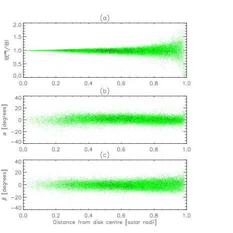
Figure 4.: The corrected dependence of knot parameters on the distance to the solar disk center ($k=0.565$):(a) - $|B_{r}^{LOS}|/|{\bf B}|$ ; (b) - $\alpha$, (c) - $\beta$; green - for the full set of magnetograms, black - points of one magnetogram SDO/HMI 2012-01-15 05:12:00 UT. SA (non-corrected magnetogramkfig4

We observe that only this value dispersion depends on the distance to the solar disk center. In addition, the second knot parameter $\alpha$ dependence on the distance to the center of the solar disk disappears, too. In fact, pursuant to the $\alpha$ definition, from (keq2) we can predict its behavior on the disk (before correction), believing $\beta=0$:

$$\ilabel{keq10}\alpha=\arccos\left((1-kr_{\perp})(1-r^{2}_{\perp})-r_{\perp}\sqrt{1-(1-kr_{\perp})^{2}(1-r^{2}_{\perp})}\right).$$ (10)

Figure kfig3 (b) depicts dependence of (keq10) with a dashed line for $k=0.565$. It is clear that with the disappearance of (keq2) dependence, the average $\alpha$ must be zero everywhere.

Despite the fact that the correction with the selected value $k$ led to an improvement in the behavior of the knots parameters on the disk (Figure kfig4), it is not completely correct. For selection of the knot regions in SA we used the non-corrected (”wrong”) values of the field modulus, which changes significantly with the correction as we determined. Hence, the knot parameters obtained from the corrected magnetogram for $k=0.565$ give the results with some residual statistical dependence on the distance, near the limb (see Figure kfig5).

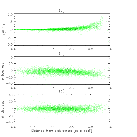
Figure 5.: The corrected dependence of knot parameters on the distance to the solar disk center ($k=0.565$):(a) - $|B_{r}^{LOS}|/|{\bf B}|$ ; (b) - $\alpha$, (c) - $\beta$; green - for the full set of magnetograms, black - points of one magnetogram SDO / HMI 2012-01-15 05:12:00 UT. SA (corrected magnetogram)kfig5

This result is quite natural, because the obtained fitting-valuek was derived from the set of ”wrong magnetograms”. As a result of selection we found $k=0.4$ as the most appropriate value (solid line in Figure. kfig3 (a)). As Figure kfig6 shows, correction with the derived $k$ value factually takes off the knot parameters dependence on the distance to the solar disk center. Figure kfig3 (b) shows dependence (keq10) corresponding to this value $k$ as a solid line. It is natural that the latter is a bit offset from the $\alpha$ knot parameter averages.

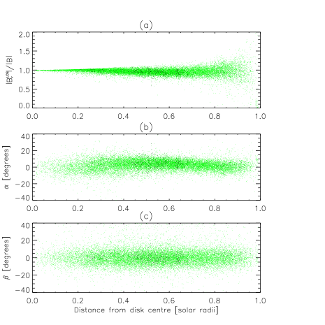
Figure 6.: The corrected dependence of knot parameters on the distance to the solar disk center ($k=0.4$):(a) - $|B_{r}^{LOS}|/|{\bf B}|$ ; (b) - $\alpha$, (c) - $\beta$; green - for the full set of magnetograms, black - points of one magnetogram SDO / HMI 2012-01-15 05:12:00 UT. SA (corrected magnetogram)kfig6

So, we have magnetograms whose knot fields satisfy the natural assumption of radiality. In any point of magnetogram, changes in modulus and inclination depend only on the $\gamma$ local value, according to formulas (keq8), (keq9) for $k=0.4$. These variations change inclinations and magnetic field significantly (see Figure kfig7).

Figure 7.: Plots that depict variations in inclination (a) and field modulus (b) after correctionkfig7

Only results of application solutions of physical problems can later allow us to assess how legitimate such correction is for magnetic parameters in active regions, because in a general way, we do not have any assumptions about true orientation of the magnetic field.

3.3 Correspondence of Magnetograms With the Force-free Approximation

S3.3 Some feature of the proposed correction can be given on the basis of the assumed force-free nature of magnetic field. At photospheric heights, this assumption must be approximately fulfilled at least for the regions with strong magnetic field. In force-free approximation, the virial theorem is valid, it gives the full energy equation as the surface integral for the entire Sun sphere (see Livshits et al. (2015)):

$$\ilabel{keq11}E\equiv\frac{1}{4\pi}\int_{V}|{\bf B}|^{2}dv=E_{vir}=\frac{R_{sun}}{8\pi}\int_{S}(B^{2}_{r}-B^{2}_{t})ds,$$ (11)

where $B_{t}$ is a tangential component of magnetic field.

As discussed in paper by Livshits et al. (2015), minimal energy of reference potential field ($B_{r}^{pot}=B_{r}$) means that any non-linear field has a greater radiality relative to its reference field:

$$\ilabel{keq12}\int_{S}B^{2}_{t}ds<\int_{S}(B^{pot}_{t})^{2}ds,$$ (12)

Calculating the integrals (keq12), we can check to what extent the original and corrected magnetograms satisfy condition (keq12), and energy positivity condition (keq11) (we shall call $E_{vir}$ virial energy). It should be noted that the appropriate testing is quite conditional, for the following reasons:
– restriction due to integration only on the visible part of the sphere;
– high noise of transverse field measurements;
– errors related to principle impossibility to solve the problem of transverse field $\pi$-uncertainty in weak fields of quiet Sun regions due to high noise;
– mainly a non-force-free nature of the field in weak field regions.

Despite the listed restrictions of such testing, the results presented in Figure kfig8, in our view, still prove specific positive features of magnetogram correction that we offer.

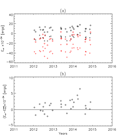
Figure 8.: (a) - calculated magnitudes of virial energies for the full set of magnetograms,$E_{vir}$- crosses,$E_{vir}(|{\bf(B)}|>150$ $erg)$ - rombs, red - non-corrected magnetograms, black - corrected magnetograms ($k=0.4$); (b) - ”free energy”.kfig8

We see that original magnetograms mainly provide ”wrong” negative magnitudes of virial energy (both for full magnetograms and these with cutting condition $|{\bf(B)}|>150$ $erg)$ to eliminate the noise). In case the noise is cut, the magnetograms after correction demonstrate ”valid” positive values of virial energy, in most cases these values exceed potential energy. It is interesting to note that the cases of ”free energy” negative values show magnetograms with ”cut” active regions – ascendant or descendant within the visibility region.

4 Conclusion

S4

We have shown that the vector magnetic data from Helioseysmic magnetic imager on-board Solar dynamic observatory (SDO/HMI) contain significant systematic error. It becomes apparent in the fact that the magnetic field in small-scale magnetic elements with high field intensity (magnetic knots) deviates from the radial direction toward the solar limb. The deviation value depends on the distance to the center of the visible solar disk and reaches maximum of $\sim 20$ degrees at distances of about $0.4$ of the solar radius to the disk center.

We offer the correction that eliminates the revealed systematic error. This correction is preliminary and requires further approbation on specific application problems. Perhaps it can serve to find causes of the data systematic error and to eliminate this error at the hardware level.

Acknowledgments

This study was supported by the Russian Foundation of Basic Research under grants 15-02-01077; was supported by the Program of basic research of the RAS Presidium No. 7.

Disclosure of Potential Conflicts of Interest

The authors declare that they have no conflicts of interest.

References

- Gosain et al. (2013) Gosain, S., Pevtsov, A. A., Rudenko, G. V., Anfinogentov, S. A.: 2013, ApJ 772, 52. doi:10.1088/0004-637X/772/1/52
- Harvey et al. (1980) Harvey, J., Gillespie, B., Miedaner, P., Slaughter, C.: 1980, NASA STI/Recon Technical Report No., 81, 21003
- Leka et al. (2017) Leka, K. D., Barnes, G., Wagner, E. L.: 2017, Sol. Phys. 292, 36.
- Livshits et al. (2015) Livshits, M. A., Rudenko, G. V., Katsova, M. M., Myshyakov, I. I.: 2017, Adv. Space Res. 55, 920. doi:10.1016/j.asr.2014.08.026
- Riley et al. (2006) Riley, P., Linker, J. A., Miki’c, Z., Lionello, R., Ledvina, S. A., Luhmann, J. G.: 2006, ApJ 653, 1510. doi:1510. doi:10.1086/508565
- Riley et al. (2014) Riley, P., Ben-Nun, M., Linker, J. A., Miki’c, Z., Svalgaard, L., Harvey, J., Bertello, L., Hoeksema, T., Liu, Y., Ulrich, R.: 2014, Sol. Phys. 289, 769. doi:10.1007/s11207-013-0353-1
- Rudenko and Anfinogentov (2014) Rudenko, G. V., Anfinogentov, S. A.: 2014, Sol. Phys. 289, 1499. doi:10.1007/s11207-013-0437-y
- Sun et al. (2012) Sun, X., Hoeksema, J. T., Liu, Y., Wiegelmann, T., Hayashi, K., Chen, Q., Thalmann, J.: 2012, ApJ 748, 77.
- Svalgaard et al. (1978) Svalgaard, L., Duvall, T. L. Jr., Scherrer, P. H.: 1978, Sol. Phys. 58, 225. doi:10.1007/BF00157268
- Tadesse et al. (2013) Tadesse, T., Wiegelmann, T., Inhester, B., et al: 2013, A&A 550, A14.
- Thalmann et al. (2012) Thalmann, J. K., Pietarila, A., Sun, X., Wiegelmann, T.: 2012, AJ 144, 33.
- Wang and Sheeley (1992) Wang, Y., Sheeley, J. N. R.: 1992, ApJ 392, 310. doi:10.1086/171430