Triangulated Surface Denoising using High Order Regularization with Dynamic Weights

Abstract

Recovering high quality surfaces from noisy triangulated surfaces is a fundamental important problem in geometry processing. Sharp features including edges and corners can not be well preserved in most existing denoising methods except the recent total variation (TV) and $\ell_{0}$ regularization methods. However, these two methods have suffered producing staircase artifacts in smooth regions. In this paper, we first introduce a second order regularization method for restoring a surface normal vector field, and then propose a new vertex updating scheme to recover the desired surface according to the restored surface normal field. The proposed model can preserve sharp features and simultaneously suppress the staircase effects in smooth regions which overcomes the drawback of the first order models. In addition, the new vertex updating scheme can prevent ambiguities introduced in existing vertex updating methods. Numerically, the proposed high order model is solved by the augmented Lagrangian method with a dynamic weighting strategy. Intensive numerical experiments on a variety of surfaces demonstrate the superiority of our method by visually and quantitatively.

65K10, 65D25, 65D18, 68U05

1 Introduction

Triangulated surfaces are used in a variety of fields, such as computer graphics [5], computer-aided design [2], computer vision [8] and many others [32, 31, 33]. Triangulated surfaces are usually generated by some digital scanner devices or triangulation algorithms [38]. However, even with high-fidelity scanners, the scanning process inevitably produces noise due to local measurement errors [29]. Such noise affects the quality of surfaces and usually cause errors in downstream geometry applications, such as surface reconstruction, segmentation and visualization [55]. Thus, how to effectively remove noise to recover high quality surfaces is one of the most fundamental tasks in geometry processing. In practice, it is difficult to distinguish noise and sharp features as they are of high frequency information. Meanwhile, it is also important to preserve smooth regions such as quadratic patches. Therefore, it is still quite challenging to remove noise while preserving sharp features and smoothly curved regions.

Filtering schemes, which can be roughly classified into two categories (isotropic and anisotropic methods), are widely applied in surface denoising. The isotropic methods [24, 53, 18, 42] are classical and simple, among which Laplacian smoothing [24] is typical. Laplacian smoothing is the process of reducing the surface area. It smoothes the surface to remove the noise without considering surface geometric features. Thus, it, as well as other isotropic methods, suffers surface shrinkage and blurs geometric features. Later on, a variety of anisotropic methods [16, 19, 1, 25, 30, 67, 50] were proposed to provide geometric features preservation. Compared to the isotropic methods, the anisotropic methods are more effective for preserving geometric features. However, when the noise level increases, the anisotropic methods usually fail to produce satisfactory results. Especially, this drawback is more severe for surfaces containing sharp features.

Variational methods are another kind of techniques for triangulated surface denoising proposed recently. To keep the sharp features, the variational models use sparsity regularization term. Inspired by the great success of total variation (TV) regularization in image processing [46], several researchers extended it to triangluated surface denoising. The authors of [23] presented an analogue of TV by minimizing the absolute value of Gauss curvature. Very recently, Zhang et al. proposed in [64] a vectorial TV based model on face normal field over triangulated surfaces. This method achieved impressive results for preserving sharp features. Another sparsity regularization is $\ell_{0}$ quasi-norm. Indeed, He and Schaefer [27] extended $\ell_{0}$ minimization [59] to triangulated surfaces for preserving sharp features. These methods achieve impressive results for surfaces consisting of flat regions and sharp features, e.g., polyhedron surfaces. However, if a surface has smoothly curved regions, they tend to flatten the smooth regions. The reason is the staircase effect of the sparsity regularization in the gradient field. The staircase effect of TV in image processing has been studied both from a theoretical and experimental points in previous works; see [12, 13, 39, 40, 41] and references therein. To overcome this disadvantage of TV, high order PDEs [48, 39, 28, 3, 35] and combination methods of TV and high order models [12, 63, 13, 39, 40, 28, 14, 45] have been used in image processing community. However, to our best knowledge, very few of high order models or combinations are known over triangulated surfaces.

Wavelet frame methods have been successfully applied in image restoration [9, 10]. Recently, Dong et al. [22, 21, 20] extended the wavelet frame methods to triangulated surfaces. Their tight wavelet frame systems are potentially effective in many geometry applications, such as denoising and semi-supervised clustering. Especially, for surface denoising, Dong et al. [21] proposed multiscale representation of surfaces using wavelet frames, which can achieve impressive denoising results for piecewise smooth surfaces with multiscale details. Yang and Wang [61] proposed a wavelet frame based variational model in [61]. Their method can effectively remove mixed Gaussian and impulse noise for the $\ell_{1}+\ell_{2}$ fidelity term of their model. However, the existing wavelet frame based methods have difficulty to recover surfaces consisting of sharp features.

Among the methods mentioned above, there are some methods belonging to two-stage methods, i.e., face normal filtering followed by updating vertices [54, 60, 49, 36, 51, 52, 67, 64, 65]. The difference between these two-stage methods is in their normal filtering strategies, e.g., a mean and median normal filter was applied in [60], [51] adopted trimmed quadratic weights for averaging the normals, Zhang et al. in [64] used a TV based model to filter a face normal field. All the normal filtering strategies can either deal with smooth regions or sharp features well. Moreover, all these two-stage methods use almost the same vertex updating model, which originated from Taubin [54], and has a beautiful implementation by Sun et al. [51]. When the noise level is low, the approach by Sun et al. [51] can achieve good results. However, when the noise level increases, the recovered vertex positions deviate far from those of the clean surface. In this situation, method of Sun et al. [51] suffers producing frequent foldovers. Moreover, large scale noise in random directions make the matter even worse. This is due to the method [51] neglects the orientations of triangle face normals, which leads vertex updating ambiguity problem; see Section 5 for the explanation of this ambiguity.

As we can see, the aforementioned surface denoising schemes including the filtering, variational and wavelet frame methods can either properly handle smooth regions or sharp features. However, it is still quite challenging to handle both smooth regions and sharp features well. In this paper, we propose a high order regularization model by introducing a new second order difference operator over triangulated surfaces. The proposed model with a well-designed weighting function is applied to the surface face normal field, which has crucial advantage in handling surfaces consisting of both smooth regions and sharp features. It preserves sharp features well and substantially suppresses the staircase effect. It is numerically solved by the operator splitting and augmented Lagrangian method. The weighting function enhances the sparsity of the proposed high order model and is implemented by a dynamic weights strategy. After restoring the face normals, the surface vertices should be updated to match the filtered face normals. Last but not least, a new vertex updating method is presented. Compared to the traditional vertex updating method [51], our new method can eliminate ambiguities and reconstruct much better triangulated surfaces. To summarize, the contributions of the paper are listed as follows:

• We introduce a new second order difference operator and its adjoint operator in piecewise constant function space over triangulated surfaces. To the best of our knowledge, this second order operator is firstly defined over triangulated surfaces.

• We introduce a novel normal filtering model using the second order regularization with a well-designed weighting function, which can preserve sharp features and simultaneously prevent the staircase effect in smooth regions.

• We propose a new vertex updating method to recover surface vertices. The proposed method significantly reduces foldovers compared to the existing vertex updating methods.

The rest of this paper is organized as follows. In Section 2, we briefly review TV based models in image processing and reweighted $\ell_{1}$ minimization. Section 3 provides the definitions of a new second order difference operator and two high order regularization models in piecewise constant function spaces. The differences of this second order operator and the Laplace operator are discussed at the end of Section 3. In Section 4, we present a high order regularization normal filtering model with a well-designed weighting function. An augmented Lagrangian method is applied to solve the variational model with a dynamic weights strategy. In Section 5, a new vertex updating method is introduced for recovering the vertex positions with respect to the filtered face normals. Our two-stage denoising method is discussed and compared to typical existing methods both qualitatively and quantitatively in Section 6. Section 7 concludes the paper.

2 TV Based Models and Reweighted $\ell_{1}$ Minimization

In this section, we present TV based models and reweighted $\ell_{1}$ minimization, since they are closely related to our approach.

2.1 TV, vectorial TV and high order models for images

Since the pioneering work of Rudin et al. [46], TV has been proven very successful in image processing for its excellent edge-preserving property [46, 39, 40, 35]. The TV denoising model (ROF) aims at solving

(1) $$\min\limits_{u}\int_{\mathrm{\Omega}}|\nabla u|+\frac{\alpha}{2}\int_{\mathrm{\Omega}}(u-f)^{2},$$

where $f$ is an observed noisy image, $\int_{\mathrm{\Omega}}|\nabla u|$ is the TV regularization and $\alpha$ is a positive fidelity parameter. For $\mathfrak{M}$-channel images $\mathbf{u},\mathbf{f}:\mathrm{\Omega}\rightarrow\mathbb{R}^{\mathfrak{M}}$, where $\mathbf{u}=(u_{1},u_{2},\ldots,u_{\mathfrak{M}})$ and $\mathbf{f}=(f_{1},f_{2},\ldots,f_{\mathfrak{M}})$, the model Eq. 1 can be naturally extended to its vectorial version for color image processing as follows:

(2) $$\min\limits_{\mathbf{u}}\int_{\mathrm{\Omega}}\Big{(}\sum\limits_{i=1}^{\mathfrak{M}}|\nabla u_{i}|^{2}\Big{)}^{\frac{1}{2}}+\frac{\alpha}{2}\int_{\mathrm{\Omega}}|\mathbf{u}-\mathbf{f}|^{2}.$$

The regularization of model Eq. 2 referred as vectorial TV has been discussed in [47, 4, 15, 7]. Both the objective functionals are coercive, proper, continuous, and strictly convex. Thus, the problems Eq. 1 and Eq. 2 have respectively, a unique minimizer.

A well known drawback of the above TV and vectorial TV models is the staircase effect [12, 13, 39, 40]. To overcome this, high order models such as Lysaker-Lundervold-Tai (LLT) model [39] and Total Generalized Variation (TGV) model [6], have been studied [48, 39, 28, 3, 6]. The idea is essentially to introduce high order derivatives to the energy regularization. High order models in general perform well in recovering smooth regions, but they cannot compete with TV in dealing with discontinuous edges. A natural solution is to combine TV and high order models [12, 63, 13, 39, 40, 28, 14, 45]. For examples, Lysaker and Tai [40] used a convex combination of TV with LLT [39]. In [13], Chan et al. presented a model combining a TV term with a weighted Laplacian term to reduce the staircase effect while preserving sharp edges. A model using infimal-convolution of the TV and high order term, was proposed by Chambolle and Lions in [12], in which the TV term was used to keep sharp edges while the high order term preserves smooth regions. The key of these methods is to balance the contribution of the TV and high order term. The balance is usually implemented by a weighting parameter or function, which needs to be tuned carefully.

2.2 Reweighted $\ell_{1}$ Minimization

The reweighted $\ell_{1}$ minimization was first presented by Candès et al. in [11] to enhance the sparsity in sparse signal recovery. It outperforms $\ell_{1}$ minimization in situations where substantially fewer measurements are used to recover a signal.

The key of the reweighted $\ell_{1}$ minimization is to solve a sequence of weighted $\ell_{1}$ minimization problems

(3) $$x^{(k)}=\mathrm{arg}\min\limits_{x\in\mathbb{R}^{n}}\|W^{(k)}x\|_{1}\quad\textmd{s.t.}\quad Ax=b,$$

where $W^{(k)}=\mathrm{diag}(w^{k}_{1},...,w^{k}_{n})$ is updated according to $x^{(k-1)}$. Although there are a variety of reweighted $\ell_{1}$ algorithms proposed to update the weights [11, 56, 66], as a rough rule of thumb, the weights should be inversely proportional to signal magnitudes [11]. For example, the reweighted method proposed by Candès et al. in [11] is as follows :

$$w^{k}_{i}=\frac{1}{|x^{k-1}_{i}|+\epsilon},\ i=1,...,n,\ \textmd{for}\,\epsilon>0.$$

3 Discrete High Order Regularization Models in Piecewise Constant Function Spaces Over Triangulated Surfaces

In this section, we introduce some notations followed by definitions of piecewise constant function spaces and difference operators over triangulated surfaces. The discrete high order models in piecewise constant spaces are presented and discussed.

3.1 Notations

Let $M$ be a compact triangulated surface of arbitrary topology with no degenerate triangles in $\mathbb{R}^{3}$. The set of vertices, edges and triangles of $M$ are denoted as $\{v_{i}:i=0,1,\cdots,\mathrm{V}-1\}$, $\{e_{i}:i=0,1,\cdots,\mathrm{E}-1\}$ and $\{\tau_{i}:i=0,1,\cdots,\mathrm{T}-1\}$, respectively. Here $\mathrm{V}$, $\mathrm{E}$ and $\mathrm{T}$ are the numbers of vertices, edges and triangles of $M$, respectively. If $v$ is an endpoint of an edge $e$, then we write it as $v\prec e$. Similarly, $e\prec\tau$ denotes that $e$ is an edge of a triangle $\tau$; $v\prec\tau$ denotes that $v$ is a vertex of a triangle $\tau$.

Denote the $1$-ring of the triangle $\tau_{i}$ as $D_{1}(\tau_{i})$, which is the set of the triangles sharing some common edges with $\tau_{i}$ indicated as green triangles in Fig. 1(a). Let $B_{1}(\tau_{i})=\{l_{j,\tau_{i}}:i=0,1,\cdots,\mathrm{T}-1;j=0,1,2\}$ be the set of lines connecting the barycenter and vertices of $\tau_{i}$, where $j$ counterclockwise marks the vertex contained in $\tau_{i}$. Namely, $l_{j,\tau_{i}}$ is the line connecting the barycenter of $\tau_{i}$ and the vertex marked as $j$ in $\tau_{i}$. Let $B_{2}(\tau_{i})$ be the set of lines connecting vertices of $\tau_{i}$ and barycenters of triangles in $D_{1}(\tau_{i})$ indicated as blue lines in Fig. 1(b). Write the 1-disk of the vertex $v_{i}$ as $M_{1}(v_{i})$ denoting the indices of triangles containing $v_{i}$ indicated as gray triangles in Fig. 1(c). We write the 1-neighborhood of vertex $v_{i}$ as $N_{1}(v_{i})$, which is the set of vertices connecting to $v_{i}$ indicated as orange vertices in Fig. 1(d).

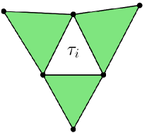
(a)

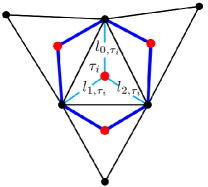
(b)

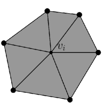
(c)

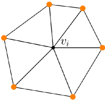
(d)

Figure 1: The illustration of $D_{1}(\tau_{i}),B_{1}(\tau_{i}),B_{2}(\tau_{i}),M_{1}(v_{i})$ and $N_{1}(v_{i})$. The elements contained in $D_{1}(\tau_{i}),B_{1}(\tau_{i}),B_{2}(\tau_{i}),M_{1}(v_{i})$ and $N_{1}(v_{i})$ are plotted in green, cyan, blue, gray and orange respectively. (a) $D_{1}(\tau_{i})$ is the 1-ring of the triangle $\tau_{i}$, which refers to $3$ triangles; (b) $B_{1}(\tau_{i})$ is the set of lines connecting the barycenter and vertices of $\tau_{i}$, which refers to $3$ lines. $B_{2}(\tau_{i})$ is the set of lines connecting vertices of $\tau_{i}$ and barycenters of triangles contained in $D_{1}(\tau_{i})$, which refers to $6$ lines; (c) $M_{1}(v_{i})$ is the 1-disk of the vertex $v_{i}$, which refers to $6$ triangles; (d) $N_{1}(v_{i})$ is the 1-neighborhood of $v_{i}$, which refers to $6$ vertices.

We further introduce the relative orientation of an edge $e$ to a triangle $\tau$, which is denoted by $\mathrm{sgn}(e,\tau)$ as follows. First, we assume that all triangles are with counterclockwise orientation and all edges are with randomly chosen fixed orientations. For an edge $e\prec\tau$, if the orientation of $e$ is consistent with the orientation of $\tau$, then $\mathrm{sgn}(e,\tau)=1$; otherwise $\mathrm{sgn}(e,\tau)=-1$.

3.2 Piecewise Constant Function Spaces and Operators

To describe piecewise constant data field, we present the concept of piecewise constant function space. Compared to piecewise linear function space which is suitable to deal with vertex-based problems, we find that, for feature preserving geometry processing [64, 37], the piecewise constant function space is more suitable which is related to piecewise constant finite element method in numerical PDE. For normal-based triangulated surface denoising, the piecewise linear function space requires the input to be vertex normals, while the input of the piecewise constant function space is face normals. The vertex normals are averaged from face normals. The second order geometry information of this smoothed vertex normal field is mush less sparse than that of the face normal field. Thus, it is more appropriate to discretize our high order regularization model in the piecewise constant function space for preserving sharp features. We should point out that, over triangulated surfaces, the second order difference operator is newly defined in this paper.

We denote the space ${V}_{M}=\mathbb{R}^{\mathrm{T}}$, which is isomorphic to the piecewise constant function space over $M$. $u=(u_{0},u_{1},\cdots,u_{\mathrm{T}-1})\in{V}_{M}$ means that the value of $u$ restricted on the triangle $\tau$ is $u_{\tau}$, which is written as $u|_{\tau}$ sometimes. The inner product and norm in $V_{M}$ are as follows:

(4) $$(u^{1},u^{2})_{{V}_{M}}=\sum\limits_{\tau}u^{1}|_{\tau}u^{2}|_{\tau}s_{\tau},\ \ \|u\|_{{V}_{M}}=\sqrt{(u,u)_{{V}_{M}}},\forall u^{1},u^{2},u\in{V}_{M},$$

where $s_{\tau}$ is the area of triangle $\tau$. For any $u\in{V}_{M}$, the jump of $u$ over an edge $e$ is

(7) $$[u]_{e}=\left\{\begin{array}[]{rl}\sum\limits_{\mathclap{\tau,e\prec\tau}}u|_{\tau}\mathrm{sgn}(e,\tau),&e\not\subset\partial M\\ 0,&e\subset\partial M\end{array}\right..$$

It is then natural to define the gradient operator by

(8) $$\nabla:V_{M}\rightarrow Q_{M},u\mapsto\nabla u,\ \ \nabla u|_{e}=[u]_{e},\ \forall e,\ \mathrm{for}\ u\in V_{M},$$

where $Q_{M}=\mathbb{R}^{\mathrm{E}}$ is the range of $\nabla$. The $Q_{M}$ space is equipped with the following inner product and norm:

(9) $$(q^{1},q^{2})_{Q_{M}}=\sum\limits_{e}q^{1}|_{e}q^{2}|_{e}\mathrm{len}(e),\ \ \|q\|_{Q_{M}}=\sqrt{(q,q)_{Q_{M}}},$$

for $q^{1},q^{2},q\in Q_{M}$, where $\mathrm{len}(e)$ is the length of the edge $e$.

It is straightforward to derive the adjoint operator of $-\nabla$, the divergence operator $\mathrm{div}:\ Q_{M}\rightarrow V_{M},q\mapsto\mathrm{div}q$, using the above inner products in $V_{M}$ and $Q_{M}$. For $q\in Q_{M}$, $\mathrm{div}q$ is given by

(10) $$(\mathrm{div}q)|_{\tau}=-\frac{1}{s_{\tau}}\sum\limits_{\begin{subarray}{c}e\prec\tau,\\ e\not\subset\partial M\end{subarray}}q|_{e}\mathrm{sgn}(e,\tau)\mathrm{len}(e),\forall\tau.$$

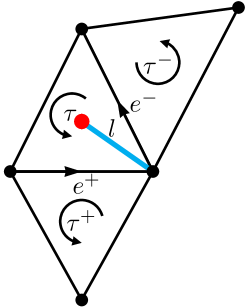
Figure 2: The illustration of the jump of $[u]_{e}$ over the line $l$ plotted in cyan in triangle $\tau$ with the barycenter plotted in red.

In the following section, we define a second order difference operator, which will be used to construct our high order regularization models. Let $l$ be a line connecting the barycenter and one vertex of the triangle $\tau$. The two edges of triangle $\tau$, which share the common vertex of $l$, are denoted as $e^{+}$ and $e^{-}$ respectively. The two triangles, contained in $D_{1}(\tau_{i})$ and share these two edges, are denoted as $\tau^{+}$ and $\tau^{-}$ respectively. All aforementioned descriptions are indicated in Fig. 2.

We then define the jump of $[u]_{e}$ over the line $l$ in $\tau$ as

(11) $${[[u]]}_{l}= [u]_{e^{+}}\mathrm{sgn}(e^{+},\tau^{+})+[u]_{e^{-}}\mathrm{sgn}(e^{-},\tau^{-})$$

$$= \big{(}(u_{\tau}\mathrm{sgn}(e^{+},\tau)+u_{\tau^{+}}\mathrm{sgn}(e^{+},\tau^{+}))\mathrm{sgn}(e^{+},\tau^{+})\big{)}+$$

$$\big{(}(u_{\tau}\mathrm{sgn}(e^{-},\tau)+u_{\tau^{-}}\mathrm{sgn}(e^{-},\tau^{-}))\mathrm{sgn}(e^{-},\tau^{-})\big{)}$$

$$= \big{(}u_{\tau^{+}}-u_{\tau}\big{)}+\big{(}u_{\tau^{-}}-u_{\tau}\big{)}$$

$$= u_{\tau^{+}}+u_{\tau^{-}}-2u_{\tau},$$

which is written as ${[[u]]}_{l,\tau}$ sometimes. With Neumann boundary condition, we actually have, for any $u\in V_{M}$,

(12) $$[[u]]_{l}=\left\{\begin{array}[]{rl}u_{\tau^{+}}+u_{\tau^{-}}-2u_{\tau},&e^{+}\text{ or }e^{-}\not\subset\partial M\\ 0,&e^{+}\text{ or }e^{-}\subset\partial M\end{array}\right..$$

From equation Eq. 11, we can obviously see that, the definition of $[[u]]_{l}$ is invariant under the choice of the orientation of edge $e$.

Then, the second order difference operator is defined by

(13) $$\nabla^{2}:V_{M}\rightarrow P_{M},u\mapsto\nabla^{2}u,\ \ \nabla^{2}u|_{\tau}=({[[u]]_{l_{0,\tau}}},{[[u]]_{l_{1,\tau}}},{[[u]]_{l_{2,\tau}}}),\ \forall\tau,\ \mathrm{for}\ u\in V_{M},$$

where $P_{M}=\mathbb{R}^{\mathrm{T}}\times\mathbb{R}^{\mathrm{T}}\times\mathbb{R}^{\mathrm{T}}$ is the range of $\nabla^{2}$. The $P_{M}$ space is equipped with the following inner product and norm:

(14) $$(p^{1},p^{2})_{P_{M}}=\sum\limits_{\tau}\sum\limits_{l\in B_{1}(\tau)}p^{1}|_{l}p^{2}|_{l}\mathrm{len}(l),\ \ \|p\|_{P_{M}}=\sqrt{(p,p)_{P_{M}}},$$

for $p^{1},p^{2},p\in P_{M}$, where $\mathrm{len}(l)$ is the length of line $l$.

Lemma 3.1.

The adjoint operator of $\nabla^{2}$ that, $(\nabla^{2})^{\star}:P_{M}\rightarrow V_{M},p\mapsto(\nabla^{2})^{\star}p$, has the following form:

(15) $$((\nabla^{2})^{\star}p)|_{\tau}=\frac{1}{s_{\tau}}\big{(}\sum\limits_{\mathclap{\mbox{\tiny$\begin{array}[]{c}l\in B_{2}{(\tau)},\\ e^{+}\mathrm{or}\ e^{-}\not\subset\partial M\end{array}$}}}p|_{l}\mathrm{len}(l)-\sum\limits_{\mathclap{\mbox{\tiny$\begin{array}[]{c}l\in B_{1}(\tau),\\ e^{+}\mathrm{or}\ e^{-}\not\subset\partial M\end{array}$}}}2p|_{l}\mathrm{len}(l)\big{)},\ \forall\tau,\ \mathrm{for}\ p\in P_{M}.$$

Proof 3.2.

As the definition of adjoint operator, we have

(16) $$\langle\nabla^{2}u,p\rangle_{P_{M}}=\langle u,(\nabla^{2})^{\star}p\rangle_{V_{M}}.$$

By using the inner products Eq. 14 and Eq. 4 in $P_{M}$ and $V_{M}$, Eq. 16 can be reformulated as

(17) $$\sum\limits_{\tau}\sum\limits_{l\in B_{1}{(\tau)}}[[u]]_{l}p|_{l}\mathrm{len}(l)=\sum\limits_{\tau}{u_{\tau}((\nabla^{2})^{\star}p)|_{\tau}s_{\tau}}.$$

By using Eq. 12, the left-hand side of Eq. 17 is actually

$$\sum\limits_{\tau}\sum\limits_{l\in B_{1}{(\tau)}}{[[u]]_{l}p|_{l}\mathrm{len}(l)}= \sum\limits_{\tau}\big{(}\sum\limits_{\mathclap{\mbox{\tiny$\begin{array}[]{c}l\in B_{1}{(\tau)},\\ e^{+}\text{or }e^{-}\not\subset\partial M\end{array}$}}}(u_{\tau^{+}}+u_{\tau^{-}}-2u_{\tau})p|_{l}\mathrm{len}(l)\big{)}$$

$$= \sum\limits_{\tau}\big{(}\sum\limits_{\mathclap{\mbox{\tiny$\begin{array}[]{c}l\in B_{2}{(\tau)},\\ e^{+}\text{or }e^{-}\not\subset\partial M\end{array}$}}}u_{\tau}p|_{l}\mathrm{len}(l)-\sum\limits_{\mathclap{\mbox{\tiny$\begin{array}[]{c}l\in B_{1}{(\tau)},\\ e^{+}\text{or }e^{-}\not\subset\partial M\end{array}$}}}2u_{\tau}p|_{l}\mathrm{len}(l)\big{)}$$

$$= \sum\limits_{\tau}u_{\tau}\big{(}\sum\limits_{\mathclap{\mbox{\tiny$\begin{array}[]{c}l\in B_{2}{(\tau)},\\ e^{+}\text{or }e^{-}\not\subset\partial M\end{array}$}}}p|_{l}\mathrm{len}(l)-\sum\limits_{\mathclap{\mbox{\tiny$\begin{array}[]{c}l\in B_{1}{(\tau)},\\ e^{+}\text{or }e^{-}\not\subset\partial M\end{array}$}}}2p|_{l}\mathrm{len}(l)\big{)}.$$

Therefore, we have

$$\sum\limits_{\tau}u_{\tau}\big{(}\sum\limits_{\mathclap{\mbox{\tiny$\begin{array}[]{c}l\in B_{2}{(\tau)},\\ e^{+}\text{or }e^{-}\not\subset\partial M\end{array}$}}}p|_{l}\mathrm{len}(l)-\sum\limits_{\mathclap{\mbox{\tiny$\begin{array}[]{c}l\in B_{1}{(\tau)},\\ e^{+}\text{or}e^{-}\not\subset\partial M\end{array}$}}}2p|_{l}\mathrm{len}(l)\big{)}=\sum\limits_{\tau}{u_{\tau}\big{(}((\nabla^{2})^{\star}p)|_{\tau}s_{\tau}\big{)}}.$$

Then, the assertion follows this immediately.

To handle vectorial data, we extend the above concepts to vectorial cases. Two vectorial spaces $\mathbf{V}_{M},\mathbf{P}_{M}$ are as follows:

$$\mathbf{V}_{M}=\underbrace{V_{M}\times\cdots\times V_{M}}\limits_{\mathfrak{N}},\mathbf{P}_{M}=\underbrace{P_{M}\times\cdots\times P_{M}}\limits_{\mathfrak{N}},$$

for $\mathfrak{N}$-channel data. The inner products and norms in $\mathbf{V}_{M}$ and $\mathbf{P}_{M}$ are as follows:

$$(\mathbf{u}^{1},\mathbf{u}^{2})_{\mathbf{V}_{M}}=\sum\limits_{1\leq i\leq\mathfrak{N}}(u_{i}^{1},u_{i}^{2})_{V_{M}},\ \ \|\mathbf{u}\|_{\mathbf{V}_{M}}=\sqrt{(\mathbf{u},\mathbf{u})_{\mathbf{V}_{M}}},\mathbf{u}^{1},\mathbf{u}^{2},\mathbf{u}\in\mathbf{V}_{M}$$

$$(\mathbf{p}^{1},\mathbf{p}^{2})_{\mathbf{P}_{M}}=\sum\limits_{1\leq i\leq\mathfrak{N}}(p_{i}^{1},p_{i}^{2})_{P_{M}},\ \ \|\mathbf{p}\|_{\mathbf{P}_{M}}=\sqrt{(\mathbf{p},\mathbf{p})_{\mathbf{P}_{M}}},\mathbf{p}^{1},\mathbf{p}^{2},\mathbf{p}\in\mathbf{P}_{M}.$$

We mention that $\nabla\mathbf{u},\nabla^{2}\mathbf{u}$ and their adjoint operators can be computed channel by channel.

3.3 Two Discrete High Order Models Over Triangulated Surfaces

Assume $f\in V_{M}$ be an observed noisy scalar field on $M$. A high order regularization model reads

(18) $$\min\limits_{u\in V_{M}}\{E_{\mathrm{ho}}(u)=R_{\mathrm{ho}}(\nabla^{2}u)+\frac{\alpha}{2}\left\|u-f\right\|^{2}_{V_{M}}\},$$

where

$$R_{\mathrm{ho}}(\nabla^{2}u)=\sum\limits_{\tau}\sum\limits_{l\in B_{1}{(\tau)}}\big{|}[[u]]_{l}\big{|}\mathrm{len}(l)=\sum\limits_{l}\big{|}[[u]]_{l}\big{|}\mathrm{len}(l),$$

is the second order variation of $u$, and $\alpha$ is a positive fidelity parameter. The minimization problem Eq. 18 has a unique minimizer under the assumption of no degenerate triangles on $M$.

Our second discrete high order regularization model is for vector field denoising over surfaces. Suppose $\mathbf{f}=(f_{1},f_{2},...,f_{\mathfrak{N}})$ be an observed noisy vector field. The vectorial version of Eq. 18 reads

(19) $$\min\limits_{\mathbf{u}\in\mathbf{V}_{M}}\{E_{\mathrm{vho}}(\mathbf{u})=R_{\mathrm{vho}}(\nabla^{2}\mathbf{u})+\frac{\alpha}{2}\left\|\mathbf{u}-\mathbf{f}\right\|^{2}_{\mathbf{V}_{M}}\},$$

where

$$R_{\mathrm{vho}}(\nabla^{2}\mathbf{u})=\sum\limits_{\tau}\sum\limits_{l\in B_{1}{(\tau)}}\Big{(}\sum\limits_{i=1}^{\mathfrak{N}}\big{|}[[u_{i}]]_{l}\big{|}|^{2}\Big{)}^{\frac{1}{2}}\mathrm{len}(l)=\sum\limits_{l}\Big{(}\sum\limits_{i=1}^{\mathfrak{N}}\big{|}[[u_{i}]]_{l}\big{|}|^{2}\Big{)}^{\frac{1}{2}}\mathrm{len}(l),$$

is the vectorial high order semi-norm.

3.4 A Discussion On the Second Order Difference and Laplace Operator

The Laplacian is the mostly frequently used high order operator in geometry processing. Of course, it can also be used to construct high order regularization model. In this subsection, we discuss differences between the second order difference operator Eq. 13 and Laplace operator in piecewise constant function space over triangulated surfaces. The high order regularization models using these two high order operators are also compared.

For clarity, we firstly give the discretization of Laplace operator in piecewise constant function space. By using the gradient operator Eq. 8 and divergence operator Eq. 10, the Laplace operator $\mathrm{\Delta}:V_{M}\rightarrow V_{M},u\mapsto\mathrm{\Delta}u$, can be derived as:

(20) $$\mathrm{\Delta}u|_{\tau}=-\frac{1}{s_{\tau}}\sum\limits_{\begin{subarray}{c}e\prec\tau,\tau\cap\tau_{i}=e,\\ e\not\subset\partial M\end{subarray}}(u_{\tau}-u_{\tau_{i}})\mathrm{len}(e),\forall\tau.$$

For a noisy scalar field, an $\ell_{1}$-norm Laplacian regularization model reads

(21) $$\min\limits_{u\in V_{M}}\{E_{\mathrm{lap}}(u)=R_{\mathrm{lap}}(\mathrm{\Delta}u)+\frac{\alpha}{2}\left\|u-f\right\|^{2}_{V_{M}}\},$$

where the regularization term is defined as

$$R_{\mathrm{lap}}(\mathrm{\Delta}u)=\sum\limits_{\tau}\big{|}\mathrm{\Delta}u|_{\tau}\big{|}s_{\tau}.$$

As we can see, discretizations of the second order operator Eq. 13 and Laplace operator Eq. 20 are totally different. Our second order operator can be seen as a set of second order central differences defined over $l$ along three different directions in one triangle. The second order regularization term of high order model Eq. 18 is an analogue of the regularization term that

$$\int_{\mathrm{\Omega}}|u_{xx}|+|u_{yy}|dxdy$$

in 2D domain, while the Laplacian regularization term of model Eq. 21 can be seen as an analogue to

$$\int_{\mathrm{\Omega}}|u_{xx}+u_{yy}|dxdy.$$

The regularization term using second order operator Eq. 13 can be computed separately in different directions, while that using the Laplace operator Eq. 20 cannot. Compared to the $\ell_{1}$-norm Laplacian model Eq. 21, the second order regularization model Eq. 18 is more effective for recovering sharp signals over triangulated surfaces; see the comparison of vectorial implementations of these two models in Fig. 12. Moreover, the second order regularization model overcomes the staircase effect introduced by first order models.

4 Normal Filtering using High Order Model with Dynamic Weights

The recent TV [64] and $\ell_{0}$ [27] based minimization methods use the concept of sparsity of first order information to remove noise from triangulated surfaces. These methods preserve sharp features well, but suffer from the staircase effect in smooth regions inevitably. In this section, a high order normal filtering model with dynamic weighs is proposed for preserving sharp features and removing the staircase effect in smooth regions simultaneously. The dynamic weights are applied in the proposed model to significantly improve effectiveness for preserving sharp features.

4.1 High Order Normal Filtering Model with Dynamic Weights

For a given noisy surface $M^{in}$, we write the face normals as $\mathbf{N}^{in}$. To remove noise in $\mathbf{N}^{in}$ through our vectorial high order model Eq. 19 with multiple spherical constraints, we propose the following variational model:

(22) $$\min\limits_{\textbf{N}\in C_{\textbf{N}}}\{E(\textbf{N})=R_{\mathrm{vhow}}(\nabla^{2}\textbf{N})+\frac{\alpha}{2}\left\|\textbf{N}-\textbf{N}^{in}\right\|^{2}_{\mathbf{V}_{M}}\},$$

where

$$C_{\textbf{N}} =\{\textbf{N}\in\mathbf{V}_{M}:\left\|\textbf{N}_{\tau}\right\|=1,\ \forall\tau\},$$

$$R_{\mathrm{vhow}}(\nabla^{2}\textbf{N}) =\sum\limits_{l}w_{l}{\Big{(}\sum\limits_{i=1}\limits^{3}(\nabla^{2}N_{i}|_{l})^{2}\Big{)}^{\frac{1}{2}}}\mathrm{len}(l).$$

Note that $\mathbf{V}_{M}$ denotes $3$-channel $V_{M}$ here. The dynamic weight $w_{l}$ on each $l$ of triangle is defined as

(23) $$w_{l}=\exp(-\left\|\mathbf{N}_{\tau^{+}}+\mathbf{N}_{\tau^{-}}-2\mathbf{N}_{{\tau}}\right\|^{4}).$$

The weight $w_{l}$ is designed to monotonically decrease with respect to the absolute second order difference defined on $l$.

For most surfaces, the proposed vectorial high order regularization model Eq. 19 can achieve good denoising results. However, in rare cases, where the noise level is increased, the proposed model Eq. 19 may smooth some sharp features a little. Thus, we use the dynamic weights, updated with respect to the face normals in each iteration, to enhance the sparsity of our high order model for improving sharp features reconstruction. The dynamic weights scheme is inspired by Candès et al. in [11]. These dynamic weights penalize smooth regions (smoothly curved regions and flat regions) more than sharp features, which can be applied to achieve the lower-than-$\ell_{1}$-sparsity effect. In general, the combination of the high order model and the dynamic weights is able to preserve sharp features well and at the same time recover smooth regions without staircase effects.

4.2 Augmented Lagrangian Method for Solving the High Order Normal Filtering Model

It is challenging to solve the normal filtering model Eq. 22 due to the non-differentiability and nonlinear constraints. Recently, the variable splitting and augmented Lagrangian method (ALM) have attained intensive attention for their efficiency in many $\ell_{1}$ related optimization problems [43, 44, 58]. Hence, we introduce an auxiliary variable and use ALM to handle the regularization term of Eq. 22. Moreover, in each iteration of ALM, the weight Eq. 23 is updated dynamically.

We first introduce a new variable $\textbf{p}\in\mathbf{P}_{M}$ and rewrite the problem Eq. 22 as

(24) $$\min\limits_{\textbf{N}\in\mathbf{V}_{M},\textbf{p}\in\mathbf{P}_{M}}\{ R_{\mathrm{vhow}}(\textbf{p})+\frac{\alpha}{2}\left\|\textbf{N}-\textbf{N}^{in}\right\|^{2}_{\mathbf{V}_{M}}+\sigma_{C_{\mathbf{N}}}(\textbf{N})\}$$

$$\textmd{s.t.}\quad\textbf{p}=\nabla^{2}\textbf{N},$$

where

$$\sigma_{C_{\mathbf{N}}}(\textbf{N})=\left\{\begin{array}[]{rl}0,&\mathbf{N}\in C_{\mathbf{N}}\\ +\infty,&\mathbf{N}\notin C_{\mathbf{N}}.\end{array}\right.$$

Accordingly, we define the following augmented Lagrangian function

(26) $$L(\textbf{N},\textbf{p};\lambda_{\mathbf{p}})= R_{\mathrm{vhow}}(\textbf{p})+\frac{\alpha}{2}\left\|\textbf{N}-\textbf{N}^{in}\right\|^{2}_{\mathbf{V}_{M}}+\sigma_{C_{\mathbf{N}}}(\textbf{N})$$

$$+{(\lambda_{\mathbf{p}},\textbf{p}-\nabla^{2}\textbf{N})}_{\mathbf{P}_{M}}+\frac{r_{\mathbf{p}}}{2}\|\textbf{p}-\nabla^{2}\textbf{N}\|^{2}_{\mathbf{P}_{M}},$$

where $\lambda_{\mathbf{p}}$ is a Lagrange multiplier and $r_{\mathbf{p}}$ is a positive real number. This primal variables update procedure can be separated into two subproblems:

• The $\mathbf{N}$-sub problem: given p

  (27) $$\min\limits_{\mathbf{N}\in\mathbf{V}_{M}}\frac{\alpha}{2}\|\mathbf{N}-\mathbf{N}^{in}\|^{2}_{\mathbf{V}_{M}}+(\lambda_{\mathbf{p}},-\nabla^{2}\mathbf{N})_{\mathbf{P}_{M}}+\frac{r_{\mathbf{p}}}{2}\|\mathbf{p}-\nabla^{2}{\mathbf{N}}\|^{2}_{\mathbf{P}_{M}}+\sigma_{C_{\mathbf{N}}}(\textbf{N});$$

• The $\mathbf{p}$-sub problem: given N

  (28) $$\min\limits_{\mathbf{p}\in\mathbf{P}_{M}}R_{\mathrm{vhow}}(\mathbf{p})+(\lambda_{\mathbf{p}},\mathbf{p})_{\mathbf{P}_{M}}+\frac{r_{\mathbf{p}}}{2}\|\mathbf{p}-\nabla^{2}\mathbf{N}\|^{2}_{\mathbf{P}_{M}}.$$

The $\mathbf{N}$-sub problem is a quadratic minimization with orthogonality constraints. An iterative method is needed to find its exact solution [26, 57, 34]. Due to error forgetting and cancellation properties of ALM for $\ell_{1}$ minimization problem [62], the sub-optimization problem Eq. 27 does not have to be solved very accurately. Here we adopt an approximate strategy to balance the precision and computational efficiency. We first ignore $\sigma_{C_{\mathbf{N}}}(\textbf{N})$ and solve a quadratic programming and then project the minimizer to an unit sphere. The quadratic problem (without constraints) has the first order optimality condition

(29) $$r_{\mathbf{p}}((\nabla^{2})^{\star}\mathbf{\nabla^{2}N})+\alpha\mathbf{N}=r_{\mathbf{p}}((\nabla^{2})^{\star}\mathbf{p})+(\nabla^{2})^{\star}\lambda_{\mathbf{p}}+\alpha\mathbf{N}^{in}.$$

This equation can be reformulated into a sparse and positive semidefinite linear system, which can be solved by various well-developed numerical packages. Here we use conjugate gradient (CG) method to solve the problem. The maximum number of iteration of CG method is set to be $10$ for efficiency. Then, we directly project the solution onto the unit sphere.

Next, we solve the $\mathbf{p}$-sub problem Eq. 28. By Eq. 14, this problem can be written as

(30) $$\min\limits_{\mathbf{p}}\sum_{l}w_{l}|\mathbf{p}_{l}|\mathrm{len}(l)+\sum_{l}(\lambda_{p_{l}},\mathbf{p}_{l})\mathrm{len}(l)+\sum_{l}\frac{r_{\mathbf{p}}}{2}|\mathbf{p}_{l}-(\nabla^{2}\mathbf{N})|_{l}|^{2}\mathrm{len}(l).$$

The problem Eq. 30 is decoupled and can be solved line-by-line. For each line $l$ connecting the barycenter and one vertex of one triangle, we need to solve

$$\min\limits_{\mathbf{p}_{l}}w_{l}|\mathbf{p}_{l}|+(\lambda_{p_{l}},\mathbf{p}_{l})+\frac{r_{\mathbf{p}}}{2}|\mathbf{p}_{l}-(\nabla^{2}\mathbf{N})|_{l}|^{2},$$

which has a closed form solution

(31) $$\textbf{p}_{l}=\left\{\begin{array}[]{rl}(1-\frac{1}{r_{\mathbf{p}}|\xi_{l}|})\xi_{l},&|\xi_{l}|>\frac{w_{l}}{r}\\ 0,&|\xi_{l}|\leq\frac{w_{l}}{r},\end{array}\right.$$

with

$$\xi=\nabla^{2}\mathbf{N}-\frac{\lambda_{\mathbf{p}}}{r_{\mathbf{p}}}.$$

In summary, the algorithm of high order normal filtering model Eq. 22 is given in Algorithm 1. Based on the variable splitting and ALM, this algorithm solves the non-differentiability problem with nonconvex constraints by iterating several simple operations. We should point out that, in the conventional reweighted $\ell_{1}$ minimization Eq. 3, the minimization problem with fixed weights is usually solved exactly. Therefore, the reweighted strategy is time-consuming. In contrast, Algorithm 1 updates the weights in each iteration. It can be regarded as an inexact but more efficient version of the conventional reweighted minimization algorithm. Although we currently cannot give a rigorous proof of convergence for Algorithm 1, our numerical experiments strongly validate it in practice. A theoretical analysis of this algorithm is worthy of the future research.

Algorithm 1 Augmented Lagrangian Method for High Order Normal Filtering with Dynamic Weights

1:Initialization: $\lambda^{0}_{\mathbf{p}}=0$, $\mathbf{N}^{-1}=0$, $\mathbf{P}^{-1}=0$, $k=0$, $K=100$, $\epsilon=1e-4$

2:do

3:     1. Compute $\mathbf{N}^{k}$ from Eq. 29, for fixed ($\lambda_{\mathbf{p}}^{k}$, $\mathbf{p}^{k-1}$); Normalize $\mathbf{N}^{k}$

4:     2. Compute $\mathbf{p}^{k}$ from Eq. 31, for fixed $(\lambda^{k}_{\mathbf{p}},\mathbf{N}^{k})$

5:     3. Update Lagrange multiplier $\lambda^{k+1}_{\mathbf{p}}=\lambda^{k}_{\mathbf{p}}+r_{\mathbf{p}}(\mathbf{p}^{k}-\nabla^{2}\mathbf{N}^{k})$

6:     4. Update each weight $w_{l}$ through Eq. 23 with respect to $\mathbf{N}^{k}$

7:while $\|\mathbf{N}^{k}-\mathbf{N}^{k-1}\|_{\mathbf{V}_{M}}<\epsilon$ or $k>K$

8:return $\mathbf{N}$

5 Folding Free Vertex Updating Method

After restoring the face normal field by Algorithm 1, the positions of vertices need to be reconstructed to match the updated face normals. As mentioned in Section 1, all the existing two-stage methods [54, 60, 49, 36, 51, 52, 67, 64, 65] use the same vertex updating model

(32) $$\min\limits_{v}\sum\limits_{\tau}\sum\limits_{(v_{i},v_{j})\in\tau}s_{\tau}(\mathbf{N}_{\tau}\cdot(v_{i}-v_{j}))^{2},$$

where $s_{\tau}$ is the area and $\mathbf{N}_{\tau}$ is the filtered normal of $\tau$. The gradient descent method is used to minimize this optimization problem, where its initialization is the restored face normal field. This optimization problem is to penalize the non-orthogonality between the filtered face normal and the three edges at each face over the surface. However, when a surface is corrupted by noise in random directions, the vertex updating method [51] usually produces foldings, even with the exact (ground truth) face normals. In addition, large scale noise make this phenomenon even worse; see the second column of Fig. 3. The reason is that the model Eq. 32 only penalizes the non-orthogonality and can not distinguish $-\mathbf{N}_{\tau}$ and $\mathbf{N}_{\tau}$. Thus, the model neglects the orientations of triangle face normals and leads to updating ambiguities. In other words, a vertex $v_{i}$ of triangle $\tau$ may be updated along the direction $-\mathbf{N}_{\tau}$ instead of $\mathbf{N}_{\tau}$. These triangle-wise orientation ambiguities cause inconsistent normal vectors crossing different triangles.

To address the orientation ambiguity problem, we propose a new vertex updating method, which reconstructs the surface from a given normal vector field by solving the following minimization problem:

(33) $$\min\limits_{v}\{E(v)=-\sum\limits_{\mathclap{\footnotesize\mbox{$\tau=(v_{i},v_{j},v_{k})$}}}{s_{\tau}\mathbf{N}}_{\tau}\cdot\left(\frac{(v_{j}-v_{i})\times(v_{k}-v_{i})}{\left\|(v_{j}-v_{i})\times(v_{k}-v_{i})\right\|}\right)+\frac{\eta}{2}||v-v^{in}||^{2}\},$$

where $(v_{i},v_{j},v_{k})$ are vertices of $\tau$ with counterclockwise order and $\eta$ is a small positive parameter. The first term of Eq. 33 is used to solve the orientation ambiguity problem. This term not only considers the orthogonality between the triangle face and its corresponding normal direction, but also takes into account the orientation of the face. Thus, compared to Eq. 32, the energy of model Eq. 33 poses no ambiguity. The second term of Eq. 33 is a fidelity term.

The partial derivatives of the energy $E(v)$ with respect to $v_{i}$ is as follows:

$$\nabla_{v_{i}}E(v) =$$

$$-\sum\limits_{\mathclap{\mbox{\scriptsize$\begin{array}[]{c}\tau\in M_{1}(v_{i}),\\ \tau=(v_{i},v_{j},v_{k})\end{array}$}}}s_{\tau} \bigg{(}\frac{\mathbf{N}_{\tau}\times(v_{k}-v_{j})}{\left\|(v_{j}-v_{i})\times(v_{k}-v_{i})\right\|}+\frac{\mathbf{N}_{\tau}\times(v_{k}-v_{j})}{\left\|(v_{k}-v_{j})\times(v_{i}-v_{j})\right\|}+\frac{\mathbf{N}_{\tau}\times(v_{k}-v_{j})}{\left\|(v_{i}-v_{k})\times(v_{j}-v_{k})\right\|}$$

$$-\frac{\mathbf{N}_{\tau}\cdot\left[(v_{j}-v_{i})\times(v_{k}-v_{j})\right]\left[(v_{j}-v_{i})\times(v_{k}-v_{i})\times(v_{k}-v_{j})\right]}{{\left\|(v_{j}-v_{i})\times(v_{k}-v_{i})\right\|}^{3}}$$

$$-\frac{\mathbf{N}_{\tau}\cdot\left[(v_{k}-v_{j})\times(v_{i}-v_{j})\right]\left[(v_{k}-v_{j})\times(v_{i}-v_{j})\times(v_{k}-v_{j})\right]}{{\left\|(v_{k}-v_{j})\times(v_{i}-v_{j})\right\|}^{3}}$$

$$-\frac{\mathbf{N}_{\tau}\cdot\left[(v_{i}-v_{k})\times(v_{j}-v_{k})\right]\left[(v_{i}-v_{k})\times(v_{j}-v_{k})\times(v_{k}-v_{j})\right]}{{\left\|(v_{i}-v_{k})\times(v_{j}-v_{k})\right\|}^{3}}\bigg{)}+\eta(v_{i}-v_{i}^{in}).$$

Using the two facts that

$$\left\|(v_{j}-v_{i})\times(v_{k}-v_{i})\right\|=\left\|(v_{k}-v_{j})\times(v_{i}-v_{j})\right\|=\left\|(v_{i}-v_{k})\times(v_{j}-v_{k})\right\|=2\mathcal{S}_{\tau},$$

$$\frac{(v_{j}-v_{i})\times(v_{k}-v_{i})}{2\mathcal{S}_{\tau}}=\frac{(v_{k}-v_{j})\times(v_{i}-v_{j})}{2\mathcal{S}_{\tau}}=\frac{(v_{i}-v_{k})\times(v_{j}-v_{k})}{2\mathcal{S}_{\tau}}=\mathcal{N}_{\tau},$$

where $\mathcal{S}_{\tau}$ and $\mathcal{N}_{\tau}$ are updating area and normal of triangle $\tau$ according to the updated vertices $v$, we arrive at

(34) $$\nabla_{v_{i}}E(v)=\sum\limits_{\mathclap{\mbox{\scriptsize$\begin{array}[]{c}\tau\in M_{1}(v_{i}),\\ \tau=(v_{i},v_{j},v_{k})\end{array}$}}}\frac{3s_{\tau}((\mathbf{N}_{\tau}\cdot\mathcal{N}_{\tau})\mathcal{N}_{\tau}-\mathbf{N}_{\tau})\times(v_{k}-v_{j})}{2\mathcal{S}_{\tau}}+\eta(v_{i}-v_{i}^{in}).$$

With the given gradient information Eq. 34 and the vertex positions of the initial noisy surface, many popular optimization techniques, such as Accelerated Gradient Descent and Quasi-Newton methods, can be used to solve our model Eq. 33. In this paper, we choose the BFGS algorithm [17], which is one of the most commonly used methods for solving nonconstrained problems like Eq. 33. In each iteration, BFGS algorithm uses only the energy and gradient evaluated at the current and previous iterations.

Figure 3 demonstrates that our method Eq. 33 can greatly reduce foldovers compared to the method Eq. 32 proposed by Sun et al. [51]. From the energy evolution curves in Fig. 3, we observe that, both methods are convergent and the iteration numbers of these two are close. However, the results produced by [51] suffer from severe foldovers (highlighted in red) and are inaccurate, while our method produces much better results without foldovers.

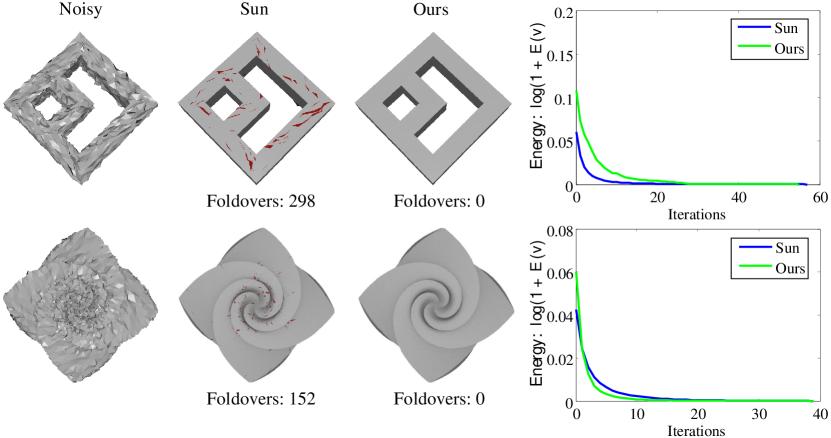
Figure 3: Comparisons of vertex updating methods (the method Eq. 32 proposed by Sun et al. [51] and ours Eq. 33). The first column shows the triangulated surfaces corrupted by Gaussian noise with standard deviation $\sigma=0.4$ mean edge length and $\sigma=0.3$ mean edge length in random directions. The second and third columns are results produced by [51] and ours, respectively. The foldovers are highlighted in red. The results produced by ours are without foldovers. The last column illustrates the energy evolution curves via iteration numbers.

6 Numerical Experiments

We verify the effectiveness of our two-stage denoising method on a variety of triangulated surfaces with either synthetic or raw noise. The synthetic noise added in random directions is produced by a zero-mean Gaussian function with standard deviation $\sigma$ proportional to the mean edge length of the clean surface. The clean surfaces tested in this section are listed in Fig. 4.

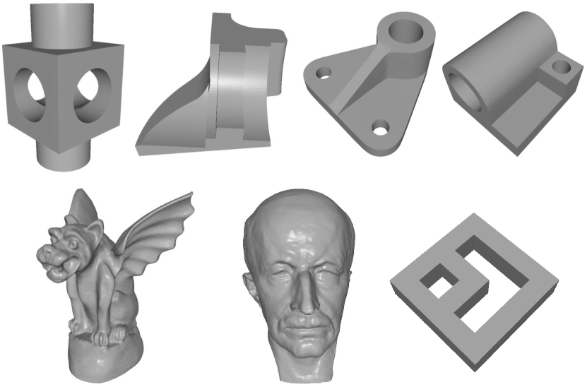
Figure 4: The clean surfaces tested in Section 6. From top left to bottom right: Block, Fandisk, Part, Joint, Gargoyle, Max-Planck and Doubletorus.

To verify the robustness of our denoising method to quality of surface triangles, we use two quantities as in [37]. These quantities are defined as following:

$$D^{global}=\frac{\mathrm{min}_{\tau}\ \mathrm{area}\ \mathrm{of}\ \tau}{\mathrm{max}_{\tau}\ \mathrm{area}\ \mathrm{of}\ \tau},$$

$$D^{local}=\min_{\tau}\frac{\min_{e\prec\tau}\ \mathrm{length\ of\ }e}{\max_{e\prec\tau}\ \mathrm{length\ of\ }e}.$$

$D^{global}$ stands for the smallest largest triangle area ratio used for globally describing the distribution of triangles. $D^{local}$ denotes the smallest one of ratios of shortest and longest edge lengths in triangles, which can be used to locally measure the quality of triangles. The information of the clean surfaces are listed in Table 1. Although several surfaces including Gargoyle, Max-Planck and Embossment are not with very regular meshes as $D^{global}$ and $D^{local}$ indicated in Table 1, our method can still effectively handle all these surfaces and produce satisfactory results.

Table 1: Information of surfaces tested in this paper

Surface	#vertices	#triangles	$D^{global}$	$D^{local}$
Block	8771	17500	0.066312	0.369025
Fandisk	6475	12946	0.0202721	0.333103
Part	4261	8530	0.0596278	0.235325
Joint	5636	11276	0.000489636	0.0508141
Gargoyle	25002	50000	0.000194802	0.0814815
Max-Planck	30942	61880	9.28547e-006	0.0135542
Rabbit	37394	73679	0.0805432	0.0991931
Angel	24566	72690	0.041708	0.0824533
Shell	58354	174031	0.00645787	0.106432
Embossment	65988	195095	0.00735766	0.0106189
Doubletorus	2686	5376	0.00439037	0.109461

For fair comparisons, we have implemented all the algorithms tested in this paper using C++ and run all examples on a notebook with a Intel dual core 2.10 GHz processor and a 8GB RAM. All the surfaces are rendered in flat-shading model to show faceting effect. Our algorithm is compared qualitatively and quantitatively to state-of-art methods, respectively. We also discuss our algorithm from various aspects, including influences of parameters and algorithm convergence.

6.1 Qualitative Comparisons

In this subsection, we compare our surface denoising method w-HO with other methods including TV normal filtering method [64], $\ell_{0}$ minimization [27] and bilateral weighting Laplacian optimization [67], abbreviated as TV, $\ell_{0}$ and bw-Laplacian respectively. For all these methods, we carefully tuned the parameters to get the visually best denoising results.

In Fig. 5, we compare the results for surfaces containing both sharp features (including sharp edges and corners) and smooth regions (including smoothly curved regions and flat regions). As we can see, bw-Laplacian keeps smooth regions well but blurs sharp features, while our w-HO method, TV and $\ell_{0}$ preserve most sharp features well. Furthermore, TV and $\ell_{0}$ both suffer from staircase effects in smoothly curved regions indicated in Fig. 5(c) and (d), and this phenomenon is extremely serious for $\ell_{0}$ which produces false edges in the first and last row of (d) of Fig. 5. However, our w-HO method does not produce the staircase effect while preserving sharp features well. As we know, both sharp features and noise belong to high frequency information. The bw-Laplacian cannot distinguish them strictly, especially for small scale features. Thus, it may treat some features as noise and blur them. In addition, as stated in compressed sensing, both $\ell_{0}$ norm and $\ell_{1}$ norm have sparse property, which can be used for preserving sharp features. However, as $\ell_{0}$ and TV use low order information of surfaces, they tend to produce staircase effects in smooth regions, especially for $\ell_{0}$ for its high sparsity requirement. Consequently, the compared three methods can either deal with smooth regions or sharp features well. In contrast, our w-HO method can suppress the staircase effects in smooth regions and simultaneously preserve sharp features. In all, for CAD-like surfaces, visual comparisons in Fig. 5 show that our w-HO method is noticeably better than all the other three methods in terms of smooth regions and sharp features recovery.

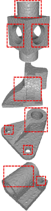
(a) Noisy

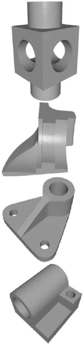
(b) w-HO

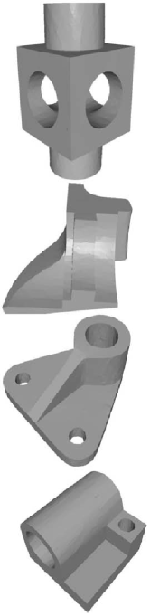
(c) TV

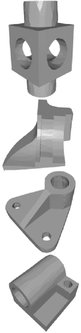
(d) $\ell_{0}$

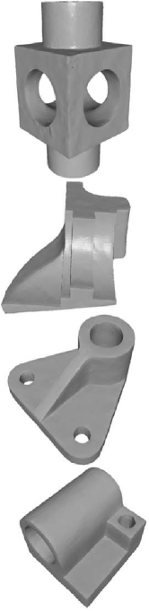
(e) bw-Laplacian

Figure 5: Denoising results of Block, Fandisk, Part and Joint (corrupted by Gaussian noise, standard deviation = 0.15 mean edge length). From left to right: input noisy surfaces, denoising results produced by our proposed w-HO method, TV method [64], $\ell_{0}$ minimization [27] and bilateral weighting Laplacian method [67], respectively.

Figure 6 shows results of surfaces with fine features. As can be seen, TV and $\ell_{0}$ tend to flatten some details, and $\ell_{0}$ performs even worse. Our w-HO method and bw-Laplacian can both generate visually better denoising results. However, from numerical metrics (which will be introduced in Section 6.2), we observe that errors of our method are always lower than those of bw-Laplacian. This demonstrates that our method is better than bw-laplacian. In general, for non-CAD surfaces, our w-HO method can also yield satisfactory results containing more details than other methods.

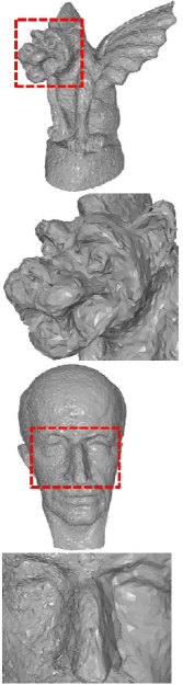
(a) Noisy

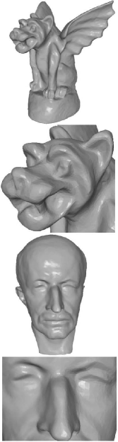
(b) w-HO

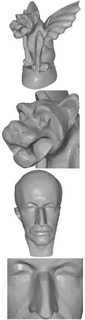
(c) TV

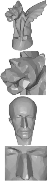
(d) $\ell_{0}$

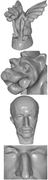
(e) bw-Laplacian

Figure 6: Denoising results of Gargoyle (corrupted by Gaussian noise, standard deviation = 0.25 mean edge length) and Max-Planck (corrupted by Gaussian noise, standard deviation = 0.2 mean edge length). From left to right: input noisy surfaces, denoising results produced by our proposed w-HO method, TV method [64], $\ell_{0}$ minimization [27] and bilateral weighting Laplacian method [67], respectively. The second and fourth rows show magnified views of Gargoyle and Max-Planck.

To further demonstrate the validity of our w-HO method, we test it on real scanned surfaces; see Fig. 7. We can see that, our method can yield very good denoising results preserving most features well.

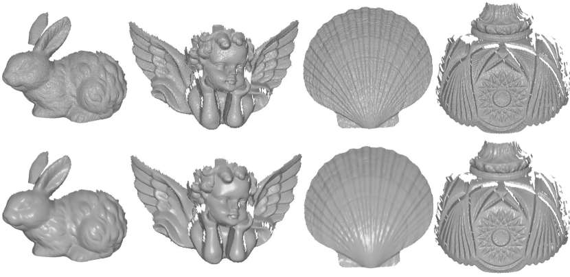
Figure 7: Our denoising results for four real scanned surfaces. From left to right: Rabbit, Angel, Shell and Embossment.

6.2 Quantitative Comparisons

Table 2: Quantitative evaluation results of Figs. 5 and 6 for our proposed w-HO method, TV method [64], $\ell_{0}$ minimization [27] and bilateral weighting Laplacian method [67]. $\sigma$ is the standard deviation of the Gaussian noise added to the clean surface.

Models	$\sigma$	Methods	$\mathrm{MSAE}$	$\mathcal{E}_{v,2}$	CPU costs
			$(\times 10^{-3})$	$(\times 10^{-3})$	(in seconds)
Block	0.15	w-HO	$\mathbf{2.40}$	$\mathbf{0.79}$	7.35
		TV	$3.61$	$0.98$	2.13
		$\ell_{0}$	$4.31$	$1.81$	16.57
		bw-Laplacian	$5.66$	$1.01$	1.45
Fandisk	0.15	w-HO	$\mathbf{1.48}$	$0.88$	1.68
		TV	$1.53$	$\mathbf{0.86}$	0.84
		$\ell_{0}$	$3.85$	$1.12$	7.53
		bw-Laplacian	$2.50$	$1.01$	0.76
Part	0.15	w-HO	$\mathbf{1.29}$	$\mathbf{0.94}$	1.84
		TV	$2.51$	$1.22$	0.67
		$\ell_{0}$	$8.1$	$2.32$	8.01
		bw-Laplacian	$4.22$	$1.23$	0.53
Joint	0.15	w-HO	$\mathbf{2.88}$	$\mathbf{0.76}$	2.80
		TV	$4.21$	$1.20$	1.98
		$\ell_{0}$	$12.7$	$2.37$	12.84
		bw-Laplacian	$6.77$	$2.01$	0.81
Bunny	0.2	w-HO	$\mathbf{12.9}$	$0.92$	18.78
		TV	$16.1$	$0.89$	8.57
		$\ell_{0}$	$27.5$	$2.16$	60.72
		bw-Laplacian	$13.4$	$\mathbf{0.88}$	7.89
Gargoyle	0.25	w-HO	$\mathbf{13.5}$	$0.77$	23.32
		TV	$17.3$	$0.83$	12.34
		$\ell_{0}$	$31.0$	$1.79$	57.36
		bw-Laplacian	$16.1$	$\mathbf{0.75}$	5.12
Max-Planck	0.2	w-HO	$\mathbf{10.8}$	$\mathbf{0.85}$	31.81
		TV	$16.6$	$1.11$	13.41
		$\ell_{0}$	$33.5$	$1.86$	74.05
		bw-Laplacian	$12.1$	$0.91$	9.41

From the above comparisons, we find that our w-HO method generates visually better results than those compared methods. In this subsection, we further compare them quantitatively.

We use two error metrics [51, 52, 67] to measure the deviation of the denoised surface from the clean one, which are defined as followed:

• Mean square angular error (MSAE):

  $$\mathrm{MSAE}=\mathrm{average}({\angle(\mathbf{N}^{{}^{\prime}},\mathbf{N})}),$$

  where $\angle(\mathbf{N}^{{}^{\prime}},\mathbf{N})$ is the square angle between the normal of the denoising result and the clean surface, $\mathrm{average}({\angle(\mathbf{N}^{{}^{\prime}},\mathbf{N})})$ is the square angle averaged over all faces.

• $L_{2}$ vertex-based surface-to-surface error:

  $$\mathcal{E}_{v,2}=\sqrt{\frac{1}{3\sum\limits_{\tau}s_{\tau}}\sum\limits^{\mathrm{V}-1}_{i=0}(\sum\limits_{M_{1}(v_{i})}s_{\tau})\mathrm{dist}(v^{,}_{i},M)^{2}},$$

  where $\mathrm{dist}(v^{,}_{i},M)$ is the distance between the updated vertex $v^{{}^{\prime}}_{i}$ and a triangle of the clean surface $M$ which is closest to $v^{{}^{\prime}}_{i}$.

Then, we compare our w-HO method to other three methods using the above two error metrics for the examples shown in Figs. 5 and 6. The evaluation results are listed in Table 2. As can be seen, our w-HO method outperforms the other methods in the sense that angular errors (MSAE) from w-HO are significantly smaller than all the other methods, especially for CAD-like surfaces. It is also observed that, the results of w-HO have the least $L_{2}$ vertex-based errors ($\mathcal{E}_{v,2}$) in most cases. This demonstrates that the results produced by w-HO are more faithful to the ground truth surfaces.

The CPU costs of all the tested methods are recorded in the last column of Table 2. For our w-HO method, the most time-consuming part is solving the N-sub problem. As mentioned in Section 4.2, due to the error forgetting property [62] of our ALM algorithm, we use a fast approximate strategy to solve this subproblem. As can be seen, bilateral weighting Laplacian method [67] is the fastest method, while $\ell_{0}$ minimization [27] is the slowest. Although our w-HO method is a little more computationally intensive than TV method [64], the CPU cost is still acceptable. In the future, we will investigate how to accelerate our w-HO method.

6.3 Influence of Parameters

To our knowledge, most triangulated surface denoising methods have parameters, which need to be manually tuned. Algorithm 1 also has two parameters, i.e., $\alpha$ and $r_{\mathbf{p}}$. These two parameters need to be tuned for producing prominent results. The first parameter is used to balance the fidelity and regularization term of the normal filtering model Eq. 22. The second one is introduced by the augmented Lagrangian method.

$\alpha$ is used to control the degree of denoising and smoothness of the result surface. Fig. 8 illustrates results of different $\alpha$ with fixed $r_{\mathbf{p}}$. As can be seen, if $\alpha$ is too large, noise cannot be effectively removed indicated in Fig. 8(b); and if $\alpha$ is too small, surfaces will be over-smoothed and fine features will be lost illustrated in Fig. 8(e). For each noisy surface, there exist a range of $\alpha$ for Algorithm 1 producing visually well denoising results; see Fig. 8(c) and (d).

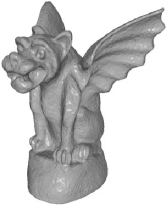
(a) Noisy

(b) $\alpha=3000$

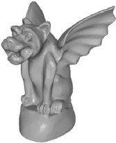
(c) $\alpha=1500$

(d) $\alpha=600$

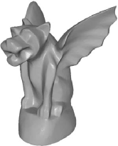
(e) $\alpha=200$

Figure 8: Denoising results for $\alpha$ with fixed $r_{\mathbf{p}}$. From left to right: input noisy surface (corrupted by Gaussian noise, standard deviation = 0.1 mean edge length) and results with different $\alpha$.

$r_{\mathbf{p}}$ also has influence on denoising results. Fig. 9 shows results of different $r_{\mathbf{p}}$ with fixed $\alpha$. As we can see, too small $r_{\mathbf{p}}$ will left some noise on the surface indicated in Fig. 9(b), and too large $r_{\mathbf{p}}$ should over-smooth the result illustrated in Fig. 9(e). Again, for each noisy surface, there exist a range of $r_{\mathbf{p}}$ for our algorithm producing visually well results as shown in Fig. 9(c) and (d).

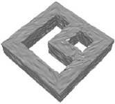
(a) Noisy

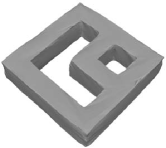
(b) $r_{\mathbf{p}}=0.1$

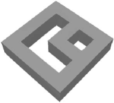
(c) $r_{\mathbf{p}}=1$

(d) $r_{\mathbf{p}}=5$

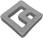
(e) $r_{\mathbf{p}}=100$

Figure 9: Denoising results for $r_{\mathbf{p}}$ with fixed $\alpha$. From left to right: input noisy surface (corrupted by Gaussian noise, standard deviation = 0.15 mean edge length) and results with different $r_{\mathbf{p}}$.

6.4 Algorithm Convergence and Effect of Dynamic Weights

Due to nonlinear and nonconvex constraints of the proposed high order normal filtering model Eq. 22, it is a challenge to have the convergence analysis of Algorithm 1. However, we can verify the convergence using numerical experiments. From the energy evolution in Fig. 10, we observe that, the energy always decrease in each iteration. This verifies the numerical convergence of Algorithm 1.

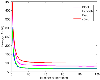
(a)

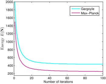
(b)

Figure 10: Energy evolution via iteration numbers of (a) surfaces in Fig. 5 and (b) surfaces in Fig. 6.

Dynamic weights in the proposed normal filtering model Eq. 22 play a good role in recovering sharp features of surfaces; see their effect in Fig. 11. As we can see, without dynamic weights, some sharp edges are smoothed a little in the denoising procedure. In contrast, the result with these dynamic weights is better.

(a) Ground truth

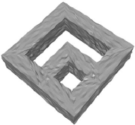
(b) noisy

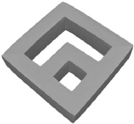
(c) result without dynamic weights

(d) result with dynamic weights

Figure 11: Denoising results of Doubletorus (corrupted by Gaussian noise, standard deviation = 0.15 mean edge length). From left to right: the clean surface, input noisy surface, denoising result produced by the proposed high order normal filtering model Eq. 22 without and with dynamic weights.

6.5 Comparison to $\ell_{1}$-norm Laplacian Normal Filtering Model

In this subsection, we compare our normal filtering model Eq. 22 with the $\ell_{1}$-norm Laplacian normal filtering model to show the advantage of our second order difference Eq. 13 over the Laplace operator Eq. 20 in surface denoising application. The $\ell_{1}$-norm laplacian normal filtering model is given as

(35) $$\min\limits_{\textbf{N}\in C_{\textbf{N}}}\{E(\textbf{N})=R_{\mathrm{vlap}}(\mathrm{\Delta}\textbf{N})+\frac{\alpha}{2}\left\|\textbf{N}-\textbf{N}^{in}\right\|^{2}_{\mathbf{V}_{M}}\},$$

where

$$C_{\textbf{N}} =\{\textbf{N}\in\mathbf{V}_{M}:\left\|\textbf{N}_{\tau}\right\|=1,\ \forall\tau\},$$

$$R_{\mathrm{vlap}}(\mathrm{\Delta}\textbf{N}) =\sum\limits_{\tau}\mathrm{w}_{\tau}{\Big{(}\sum\limits_{i=1}\limits^{3}(\mathrm{\Delta}N_{i}|_{\tau})^{2}\Big{)}^{\frac{1}{2}}}s_{\tau}.$$

The dynamic weight $\mathrm{w}_{\tau}$ on each triangle is defined as

$$\mathrm{w}_{\tau}=\exp(-\parallel\sum\limits_{\tau_{j}\in D_{1}(\tau_{i})}(\mathbf{N}_{\tau}-\mathbf{N}_{{\tau_{j}}})\parallel^{4}),$$

which is used to enhance the sparsity of the proposed model Eq. 35. For fairness, our normal filtering model Eq. 22 is compared with the Laplacian one Eq. 35 without and with dynamic weights respectively. As we can see in Fig. 12, although our normal filtering model Eq. 22 and the Laplacian model Eq. 35 both remove the staircase effect, our model Eq. 22 can preserve sharp features well while the model Eq. 35 with the Laplace operator cannot.

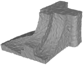
(a)

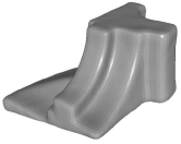
(b)

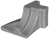
(c)

(d)

(e)

Figure 12: Denoising results of Fandisk (corrupted by Gaussian noise, standard deviation = 0.15 mean edge length). (a) is the noisy surface; (b) and (c) are results produced by $\ell_{1}$-norm Laplacian normal filtering model Eq. 35 without and with dynamic weights respectively; (d) and (e) are results produced by the high order normal filtering model Eq. 22 without and with dynamic weights respectively.

7 Conclusion

In this paper, we propose a triangulated surface denoising meth-
od using a newly defined discrete high order regularization. The method applies the high order regularization to the normal vector field with a well-designed weighting function. The variational model is solved by the augmented Lagrangian method with dynamic weights strategy. Moreover, a new vertex updating scheme is presented to overcome the orientation ambiguities introduced by previous vertex updating methods. We also compare our method to several denoising methods on a variety triangulated surfaces both qualitatively and quantitatively. Conventional methods either smooth sharp features, or generate staircase artifacts. Since our method preserves sharp features well and produces no staircase effect, it outperforms other three compared methods. Thus it can be applied to more general surfaces containing both sharp features and smoothly curved regions.

References

- [1] C. L. Bajaj and G. Xu, Anisotropic diffusion of surfaces and functions on surfaces, ACM Trans. Graph., 22 (2003), pp. 4–32.
- [2] R. E. Barnhill, Surfaces in computer aided geometric design: a survey with new results, Comput. Aided Geom. Des., 2 (1985), pp. 1–17.
- [3] M. Bergounioux and L. Piffet, A second-order model for image denoising, Set-Valued Anal., 18 (2010), pp. 277–306.
- [4] P. Blomgren and T. F. Chan, Color tv: total variation methods for restoration of vector-valued images, IEEE Trans. Image Process., 7 (1998), pp. 304–309.
- [5] M. Botsch, L. Kobbelt, M. Pauly, P. Alliez, and B. Levy, Polygon Mesh Processing, AK Peters, 2010.
- [6] K. Bredies, K. Kunisch, and T. Pock, Total generalized variation, SIAM J. Imaging Sci, 3 (2010), pp. 492–526.
- [7] X. Bresson and T. F. Chan, Fast dual minimization of the vectorial total variation norm and applications to color image processing, Inverse Probl. Imaging, 2 (2008), pp. 455–484.
- [8] A. M. Bronstein, M. M. Bronstein, and R. Kimmel, Numerical Geometry of Non-Rigid Shapes, Springer Publishing Company, Incorporated, 2008.
- [9] J. F. Cai, B. Dong, S. Osher, and Z. Shen, Image restoration: Total variation, wavelet frames, and beyond, J. AM. MATH. SOC., 25 (2012), pp. 1033–1089.
- [10] J. F. Cai, B. Dong, and Z. Shen, Image restoration: A wavelet frame based model for piecewise smooth functions and beyond, Appl. Comput. Harmon. Anal., 41 (2015), pp. 94–138.
- [11] E. J. Candès, M. B. Wakin, and S. P. Boyd, Enhancing sparsity by reweighted minimization, J. Fourier Anal. Appl., 14 (2008), pp. 877–905.
- [12] A. Chambolle and P. L. Lions, Image recovery via total variation minimization and related problems, Numer. Math., 76 (1997), pp. 167–188.
- [13] Chan, Tony, Marquina, Antonio, and Mulet, High-order total variation-based image restoration, SIAM J. Sci. Comput., 22 (2000), pp. 503–516.
- [14] T. F. Chan, S. Esedoglu, and F. Park, A fourth order dual method for staircase reduction in texture extraction and image restoration problems, in Proceedings of the 2010 IEEE International Conference on Image Processing, 2010, pp. 4137–4140.
- [15] T. F. Chan, S. H. Kang, and J. Shen, Total variation denoising and enhancement of color images based on the cb and hsv color models, J. Visual Commun. Image Represent., 12 (2001), pp. 422–435.
- [16] U. Clarenz, U. Diewald, and M. Rumpf, Anisotropic geometric diffusion in surface processing, in Processdings of the 2000 Visualization, 2000, pp. 397–405.
- [17] J. E. Dennis and J. J. More, Quasi-newton methods, motivation and theory, SIAM Rev., 19 (1977), pp. 46–89.
- [18] M. Desbrun, M. Meyer, P. Schröder, and A. H. Barr, Implicit fairing of irregular meshes using diffusion and curvature flow, in Proceedings of the 26th annual conference on Computer graphics and interactive techniques, 1999, pp. 317–324.
- [19] M. Desbrun, M. Meyer, P. Schröder, and A. H. Barr, Anisotropic feature-preserving denoising of height fields and bivariate data., in Processdings of the 2000 Graphics interface, vol. 11, 2000, pp. 145–152.
- [20] B. Dong, Sparse representation on graphs by tight wavelet frames and applications, Appl. Comput. Harmon. Anal., 42 (2017), pp. 452–479.
- [21] B. Dong, Q. Jiang, C. Liu, and Z. Shen, Multiscale representation of surfaces by tight wavelet frames with applications to denoising, Appl. Comput. Harmon. Anal., 41 (2016), pp. 561–589.
- [22] B. Dong, Y. Mao, I. D. Dinov, Z. Tu, Y. Shi, Y. Wang, and A. W. Toga, Wavelet-based representation of biological shapes, in Processdings of the 2009 International Symposium on Visual Computing, 2009, pp. 955–964.
- [23] M. Elsey and S. Esedoglu, Analogue of the total variation denoising model in the context of geometry processing, SIAM J. Multiscale Model. Simul., 7 (2009), pp. 1549–1573.
- [24] D. A. Field, Laplacian smoothing and delaunay triangulations, Commun. Appl. Numer. Methods, 4 (1988), pp. 709–712.
- [25] S. Fleishman, I. Drori, and D. Cohen-Or, Bilateral mesh denoising, ACM Trans. Graph., 22 (2003), pp. 950–953.
- [26] D. Goldfarb, Z. Wen, and W. Yin, A curvilinear search method for p-harmonic flows on spheres, SIAM J. Imaging Sci., 2 (2009), pp. 84–109.
- [27] L. He and S. Schaefer, Mesh denoising via minimization, ACM Trans. Graph., 32 (2013), pp. 1–8.
- [28] W. Hinterberger and O. Scherzer, Variational methods on the space of functions of bounded hessian for convexification and denoising, Computing, 76 (2006), pp. 109–133.
- [29] H. Hoppe, T. DeRose, T. Duchamp, J. McDonald, and W. Stuetzle, Surface reconstruction from unorganized points, in Proceedings of the 19th Annual Conference on Computer Graphics and Interactive Techniques, 1992, pp. 71–78.
- [30] T. R. Jones, F. Durand, and M. Desbrun, Non-iterative, feature-preserving mesh smoothing, ACM Trans. Graph., 22 (2003), pp. 943–949.
- [31] M. R. Kaus, J. Von Berg, J. Weese, W. Niessen, and V. Pekar, Automated segmentation of the left ventricle in cardiac mri, Med Image Anal, 8 (2004), pp. 245–254.
- [32] R. Kimmel and J. A. Sethian, Computing geodesic paths on manifolds, Proc. Natl. Acad. Sci. USA, 95 (1998), pp. 8431–8435.
- [33] R. Lai and T. F. Chan, A framework for intrinsic image processing on surfaces, Comput. Vis. Image. Und., 115 (2011), pp. 1647–1661.
- [34] R. Lai and S. Osher, A splitting method for orthogonality constrained problems, J. Sci. Comput., 58 (2014), pp. 431–449.
- [35] R. Lai, X.-C. Tai, and T. F. Chan, A ridge and corner preserving model for surface restoration, SIAM J. Sci. Comput., 35 (2013), pp. 675–695.
- [36] K. W. Lee and W. Wang, Feature-preserving mesh denoising via bilateral normal filtering, in Proceedings of the 2005 International Conference on Computer Aided Design and Computer Graphics, 2005, pp. 275–280.
- [37] Z. Liu, H. Zhang, and C. Wu, On geodesic curvature flow with level set formulation over triangulated surfaces, J. Sci. Comput., 70 (2017), pp. 631–661.
- [38] W. E. Lorensen and H. E. Cline, Marching cubes: A high resolution 3d surface construction algorithm, in Proceedings of the 14th Annual Conference on Computer Graphics and Interactive Techniques, 1987, pp. 163–169.
- [39] M. Lysaker, A. Lundervold, and X. C. Tai, Noise removal using fourth-order partial differential equation with applications to medical magnetic resonance images in space and time., IEEE Trans. Image Process., 12 (2003), pp. 1579–1590.
- [40] M. Lysaker and X. C. Tai, Iterative image restoration combining total variation minimization and a second-order functional, Int. J. Comput Vis., 66 (2006), pp. 5–18.
- [41] G. D. Maso, I. Fonseca, G. Leoni, and M. Morini, A higher order model for image restoration: the one dimensional case, SIAM J. Math. Anal., 40 (2007), pp. 2351–2391.
- [42] D. Nehab, S. Rusinkiewicz, J. Davis, and R. Ramamoorthi, Efficiently combining positions and normals for precise 3d geometry, ACM Trans. Graph., 24 (2005), pp. 536–543.
- [43] T. Oden, R. Glowinski, and P. L. Tallec, Augmented lagrangian and operator splitting method in non-linear mechanics, Math. Comput., 58 (1992).
- [44] S. Osher, M. Burger, D. Goldfarb, J. Xu, and W. Yin, An iterative regularization method for total variation-based image restoration, SIAM J. Multiscale Model. Simul., 4 (2005), pp. 460–489.
- [45] K. Papafitsoros and C. B. Schönlieb, A combined first and second order variational approach for image reconstruction, J. Math. Imaging Vis., 48 (2014), pp. 308–338.
- [46] L. Rudin, S. Osher, and E. Fatemi, Nonlinear total variation based noise removal algorithms, Physica D, 60 (1992), pp. 259–268.
- [47] G. Sapiro and D. L. Ringach, Anisotropic diffusion of multivalued images with applications to color filtering, IEEE Trans. Image Process., 5 (1996), pp. 1582–1586.
- [48] O. Scherzer, Denoising with higher order derivatives of bounded variation and an application to parameter estimation, Computing, 60 (1998), pp. 1–27.
- [49] Y. Shen and K. E. Barner, Fuzzy vector median-based surface smoothing, IEEE Trans. Vis. Comput. Graph., 10 (2004), pp. 252–265.
- [50] J. Solomon, K. Crane, A. Butscher, and C. Wojtan, A general framework for bilateral and mean shift filtering, CoRR abs/1405.4734, 8 (2014).
- [51] X. Sun, P. Rosin, R. Martin, and F. Langbein, Fast and effective feature-preserving mesh denoising, IEEE Trans. Vis. Comput. Graph., 13 (2007), pp. 925–938.
- [52] X. Sun, P. L. Rosin, R. R. Martin, and F. C. Langbein, Random walks for feature-preserving mesh denoising, Comput. Aided Geom. Des., 25 (2008), pp. 437–456.
- [53] G. Taubin, A signal processing approach to fair surface design, in Proceedings of the 22nd annual conference on Computer graphics and interactive techniques, 1995, pp. 351–358.
- [54] G. Taubin, Linear anisotropic mesh filters. IBM Research Report RC22213(W0110-051), IBM T.J. Watson Research, October 2001.
- [55] J. Wang, X. Zhang, and Z. Yu, A cascaded approach for feature-preserving surface mesh denoising, Comput-Aided Des., 44 (2012), pp. 597–610.
- [56] Y. Wang and W. Yin, Sparse signal reconstruction via iterative support detection, SIAM J. Imaging Sci, 3 (2010), pp. 462–491.
- [57] Z. Wen and W. Yin, A feasible method for optimization with orthogonality constraints, Math. Program., 142 (2013), pp. 397–434.
- [58] C. Wu and X. C. Tai, Augmented lagrangian method, dual methods, and split bregman iteration for rof, vectorial tv, and high order models, Siam J. Imaging Sci., 3 (2010), pp. 300–339.
- [59] L. Xu, C. Lu, Y. Xu, and J. Jia, Image smoothing via gradient minimization, ACM Trans. Graph., 30 (2011), p. 174.
- [60] H. Yagou, Y. Ohtake, and A. Belyaev, Mesh smoothing via mean and median filtering applied to face normals, in Geometric Modeling and Processing, 2002. Proceedings, 2002, pp. 124–131.
- [61] J. Yang and C. Wang, A wavelet frame approach for removal of mixed gaussian and impulse noise on surfaces, Inverse Probl. Imaging, 11 (2017).
- [62] W. Yin and S. Osher, Error forgetting of bregman iteration, J. Sci. Comput., 54 (2013), pp. 684–695.
- [63] Y. L. You and M. Kaveh, Fourth-order partial differential equations for noise removal., IEEE Trans. Image Process., 9 (2000), p. 1723.
- [64] H. Zhang, C. Wu, J. Zhang, and J. Deng, Variational mesh denoising using total variation and piecewise constant function space., IEEE Trans. Vis. Comput. Graph., 21 (2015), pp. 873–86.
- [65] W. Zhang, B. Deng, J. Zhang, S. Bouaziz, and L. Liu, Guided mesh normal filtering, Comput. Graph. Forum, 34 (2015), pp. 23–34.
- [66] Y. B. Zhao and D. Li, Reweighted minimization for sparse solutions to underdetermined linear systems., Siam J. Optim., 22 (2012), pp. 1065–1088.
- [67] Y. Zheng, H. Fu, K. C. Au, and C. L. Tai, Bilateral normal filtering for mesh denoising, IEEE Trans. Vis. Comput. Graph., 17 (2011), pp. 1521–1530.