Contracting Nonlinear Observers: Convex Optimization and
Learning from Data

Abstract

A new approach to design of nonlinear observers (state estimators) is proposed. The main idea is to (i) construct a convex set of dynamical systems which are contracting observers for a particular system, and (ii) optimize over this set for one which minimizes a bound on state-estimation error on a simulated noisy data set. We construct convex sets of continuous-time and discrete-time observers, as well as contracting sampled-data observers for continuous-time systems. Convex bounds for learning are constructed using Lagrangian relaxation. The utility of the proposed methods are verified using numerical simulation.

I Introduction

The problem of estimating the “internal state” (a.k.a. hidden or latent variables) of a dynamical system is one of the canonical problems in control engineering, and similar problems are encountered in time-series prediction, machine learning, signal processing, and may other fields. For linear systems a comprehensive methodology is available that combines computational simplicity, stability, and certain types of statistical or deterministic optimality (e.g. [1, 2]).

For non-linear systems, on the other hand, compromises are necessary. In all but a few isolated cases there is no finite-dimensional representation of the statistically-optimal estimator, so one must sacrifice one or more of optimality, global stability, or computational simplicity.

Extended Kalman filters retain the simple structure of the linear case, but are suboptimal and stability is generally difficult to establish [1]. More accurate but computationally intensive approaches include particle filters a.k.a. sequential Monte Carlo methods [3], Moving-horizon estimation [4], and set-valued state estimators [5]. Notably, particle filters and set-valued estimators maintain high-dimensional representations of a distribution (or set) of possible states, rather than a simple point estimate, while moving-horizon estimation maintains a long history of recorded inputs and outputs. Therefore even for low order systems, the internal state of the estimator is of high dimension.

The term “nonlinear observer” usually refers to a state estimator that abandons any claim to statistical optimality, but is a dynamical system of low dimension (equal or similar dimension to the true system), which is simple to implement, and for which global or semi-global stability can be established analytically or computationally [6].

Over the years, many methods of observer design have been developed, including those based on geometric methods [7], high-gain designs [8], immersion and invariance [9], and finding a nonlinear transformation (possibly with excessive coordinates) to a stable linear observer [10].

Computational approaches based on convex optimization (in particular, linear matrix inequalities and semidefinite programming) have been used to construct observers for systems with nonlinearities characterized by monotonicity [11, 12] and $L^{2}$ gain (e.g. [13] and references therein). Most approaches are based on the search for a quadratic Lyapunov function, while in [14] sum-of-squares programming was used to find observers for polynomial systems via certain non-quadratic Lyapunov functions. Sum-of-squares relaxes the search for sign-definite polynomials to a semidefinite program [15], and will also be applied in the present paper.

Several papers have addressed observer design using contraction analysis, e.g. [16, 17, 18]. Indeed, observer design was one of the original motivations for contraction analysis as introduced in [16]. Contraction analysis is based on the study of a nonlinear system by way of its differential dynamics (a.k.a. variational system) along solutions. Roughly speaking, since the differential dynamics are linear time-varying (LTV), many techniques from linear systems theory can be directly applied. A central result is that if all solutions of a smooth nonlinear system are locally exponentially stable in a common metric, then all solutions are globally exponentially stable. Historically, basic convergence results on contracting systems can be traced back to the results of [19] in terms of Finsler metrics, further explored in [20], while convex conditions for existence and robustness of limit cycles were given in [21], and extensions to constructive feedback design were given in [22].

In this paper we will construct convex sets of contracting observers for continuous and discrete-time nonlinear systems, as well as sampled-data observers, i.e. discrete-time observers for continuous-time systems. Sampled-data observer design is complicated by the inability to exactly solve a nonlinear differential equation over a sampling interval, and simple numerical integration techniques can cause instability [23]. We will construct sampled-data observers via trapezoidal approximation, and prove that they remain stable.

Having constructed a convex set of observers, we propose optimizing over this set to find an observer that minimizes a measure of state estimation error on a finite data set. That is, our approach is based on learning from data, and is similar to the prediction error methods in black-box nonlinear system identification [24, 25] and recurrent neural networks [26], and snapshot-based model reduction [lucia2004reduced]. The central difference is that in prediction-error method the objective is to find a dynamical model of the system, whereas in this paper we assume a dynamical model is known, and the objective is to optimize a state estimator. This could be considered a form of regularization of prediction error methods: the identified model must behave as an observer for a certain known system.

This paper builds upon a framework introduced for system identification and model reduction in [27, 28]. In particular, we make use of similar convex parameterizations of stable systems and bounds on nonlinear system behaviour as those papers. The novel contributions of this paper are: (i) we show how these techniques can be applied to the observer design problem, (ii) we provide new convex sets of models for CT systems and exponentially contracting systems, (iii) we show that trapezoidal integration of CT observers preserves stability, and (iv) we propose a method to optimize mean-square error of observers based on simulated data. The benefits of the proposed approach are illustrated using simulations.

II Preliminaries

II-A Notation

In this paper, we will consider both continuous-time (CT) and discrete-time (DT) systems and signals. Let $\mathbb{Z}^{+}$ and $\mathbb{R}^{+}$ denote the non-negative integers and reals, respectively. Let $\ell_{2}^{n}$ denote the set of square-summable signals $\mathbb{Z}^{+}\to\mathbb{R}^{n}$. Similarly, $L_{2}^{n}$ denotes the subspace of square-integrable signals $\mathbb{R}^{+}\to\mathbb{R}^{n}$. We use subscripts for time indexing, i.e. for a signal $x$, $x_{t}\in R^{n}$ denotes its value at time $t\in\mathbb{Z}^{+}$ or $\mathbb{R}^{+}$. For a symmetric matrix, $A>0$ ($A\geq 0$) denotes positive-definiteness (semidefiniteness), and $A>B$ ($A\geq B$) means $A-B>0$ ($A-B\geq 0$). For a vector $x$, $|x|$ is the Euclidean norm, and $|x|^{2}_{P}$ is shorthand for $x^{\prime}Px$ where $P>0$. We will also abuse notation slightly by using the shorthand $|H|^{2}_{P}=H^{\prime}PH$ even if $H$ is matrix with more than one column.

II-B Observer Design

In this subsection we describe the deterministic nonlinear observer design problem. In Section IV we will extend consideration to stochastic models with disturbances and measurement errors.

We consider a “true system” model with finite-dimensional state $x\in\mathbb{R}^{n}$, driven by a known input $u\in\mathbb{R}^{m}$ and producing a measured output $y\in\mathbb{R}^{p}$. The dynamic and sensor models are given by the following equations

$$\sigma x_{t}=a(x_{t},u_{t}),\quad y=g(x_{t},u_{t}),$$ (1)

where the operator $\sigma$ represents $\frac{d}{dt}$ for CT models, and the shift operator $x_{t}\mapsto x_{t+1}$ for DT models. In the CT case, for simplicity of development we will assume existence and uniqueness of solutions for all $t\in[0,\infty)$.

In this paper, an observer for (1) is another dynamical system with a state estimate as its internal state $\hat{x}\in\mathbb{R}^{n}$, which takes the input and output of (1) as its own inputs:

$$\sigma\hat{x}_{t}=\phi(\hat{x}_{t},u_{t},y_{t}),$$ (2)

While more general notions of an observer are possible with different dimension to the true system [6], for this paper we restrict attention to the simplest case when the observer’s internal state is $\hat{x}$. We will assume that the functions $a,g,\phi$ are continuously differentiable in their arguments.

The observer design problem is to find a function $\phi$ in (2) such that $\hat{x}_{t}$ is uniquely-defined on $t\in[0,\infty)$ (which we call well-posedness), and guaranteed to converge (in some sense) to $x_{t}$ as $t\rightarrow\infty$. In this paper, we will focus on the following forms of convergence:

Definition 1

System (2) is said to be an $L^{2}$ observer for (1) if for all $x_{0}\in\mathbb{R}^{n},\hat{x}_{0}\in\mathbb{R}^{n}$ $x_{t}-\hat{x}_{t}\in L_{2}^{n}$ for CT or $\ell_{2}^{n}$ for DT observers, and if $\hat{x}_{0}=x_{0}$ then $\hat{x}_{t}=x_{t}$ for all $t\geq 0$. System (2) is said to be an exponential observer with rate $\lambda>0$ if the stronger condition holds that there exists a function $b:\mathbb{R}^{n}\times\mathbb{R}^{n}\to\mathbb{R}^{+}$ with $b(x,x)=0$ for all $x$, such that for all $x_{0},\hat{x}_{0}\in\mathbb{R}^{n}$:

$$|x_{t}-\hat{x}_{t}|\leq e^{-\lambda t}b(x_{0},\hat{x}_{0}).$$ (3)

II-C Contraction Analysis

Contraction analysis [16] studies the convergence of solutions of a dynamical system to each other, rather than to a particular pre-defined “nominal” solution as in standard Lyapunov analysis. Thus stability of a system can be established independent of knowledge of a particular solution, a property which is particularly well suited to observer design.

Contraction analysis is based on the study of the differential dynamics (a.k.a. variational, linearized, prolonged), defined along solutions of a system of the form (2):

$$\sigma\delta_{t}=\frac{\partial\phi}{\partial\hat{x}}\delta_{t}.$$

A central result of [16] for the CT case is that if there exists a uniformly bounded metric $M(x)$ such that

$$\dot{M}+\frac{\partial\phi}{\partial x}^{\prime}M+M\frac{\partial\phi}{\partial x}\leq-2\lambda M,$$

where $\dot{M}=\frac{\partial M}{\partial x}\phi$, then the system is contracting with rate $\lambda$. In the DT case we have the similar condition

$$\frac{\partial\phi}{\partial x}^{\prime}M(x_{t+1})\frac{\partial\phi}{\partial x}-M(x_{t})\leq(1-e^{-\lambda})M(x_{t}).$$

II-D Bounds and Identities for Quadratic Functions

Throughout the paper we will frequently use the following simple property. Concave functions $g(c,P)=-c^{\prime}P^{-1}c$ with $c\in\mathbb{R}^{n},P=P^{\prime}>0$ obey the upper bound:

$$-c^{\prime}P^{-1}c\leq b^{\prime}Pb-2b^{\prime}c$$ (4)

where the right-hand side is a convex function of $c,P$ for any fixed $b\in\mathbb{R}^{n}$. Inequality (4) follows directly from the expansion $b^{\prime}Pb-2b^{\prime}c+c^{\prime}P^{-1}c=|c-Pb|^{2}_{P^{-1}}\geq 0.$ From this expansion it is also clear that the bound (4) is tight if $c=Pb$.

We will also frequently use the following version of the polarization identity, valid for $Q=Q^{\prime}>0$, arbitrary matrices $E,F$ of appropriate dimension, and arbitrary scalar $h>0$, which follows from expansion of the right hand side:

$$E^{\prime}QF+F^{\prime}QE=\tfrac{1}{h}\left[|E+\tfrac{h}{2}F|^{2}_{Q}-|E-\tfrac{h}{2}F|^{2}_{Q}\right].$$ (5)

III Convex Sets of Nonlinear Observers

In this paper, a system set is a pair $(\phi,\Theta)$ where $\phi:\mathbb{R}^{n}\times\mathbb{R}^{m}\times\mathbb{R}^{p}\times\mathbb{R}^{q}\rightarrow\mathbb{R}^{n}$ is a continuously differentiable function, and $\Theta\subset\mathbb{R}^{q}$ is a set of $q$-dimensional parameter vectors. Associated with $(\phi,\Theta)$ are state-space dynamical systems of the form

$$\sigma\hat{x}_{t} = \phi(\hat{x}_{t},u_{t},y_{t},\theta),$$ (6)

where $\hat{x}\in\mathbb{R}^{n},u\in\mathbb{R}^{m},y\in\mathbb{R}^{p}$, $\theta\in\Theta$.

We define a contracting observer set for a system (1) as any system set such that, for all $\theta\in\Theta$, the following two conditions are satisfied:

1. Contraction: any pair trajectories $\hat{x}^{a},\hat{x}^{b}$ of (2) with the same inputs $(u,y)$ but with different initial conditions $\hat{x}^{a}_{0},\hat{x}^{b}_{0}$ converge, in one of the following two senses

   1. $L^{2}$ contraction, i.e. $\hat{x}^{a}-\hat{x}^{b}\in L^{2}$ (or $\ell^{2}$ for DT observers).

   2. exponential contraction with rate $\lambda>0$, i.e.

      $$|\hat{x}^{a}_{0}-\hat{x}^{b}_{0}|\leq e^{-\lambda t}b(\hat{x}^{a}_{0},\hat{x}^{b}_{0}).$$ (7)

      function $b:\mathbb{R}^{n}\times\mathbb{R}^{n}\to\mathbb{R}^{+}$ with $b(x,x)=0$.

2. Correctness: when initialised with $\hat{x}_{0}=x_{0}$, the observer matches the true system, i.e. $\hat{x}_{t}=x_{t}$ for all $t\geq 0$. This is the case if and only if

   $$a(x,u)=\phi(x,u,g(x,u),\theta)\quad\forall x\in\mathbb{R}^{n},u\in\mathbb{R}^{m}.$$ (8)

In what follows, we will usually drop the $\theta$ argument, and speak directly of searching over functions $\phi(\hat{x},u,y)$.

It is obvious that these two conditions are sufficient for (2) to be an observer for (1) for any $\theta\in\Theta$: correctness implies that the true state $x$ is a particular solution of the observer, while contraction implies that all solutions of the observer converge to each other, hence all solutions of the observer converge to the true state. This characterization of a contracting observer is a special case of the idea of virtual system used to study observers and more general synchronization behaviors in [29].

III-A Convex Sets of Contracting Continuous-Time Observers

In this section we will construct convex sets of contracting nonlinear observers for CT systems of the form

$$\dot{x}_{t}=a(x_{t},u_{t}),\quad y_{t}=g(x_{t},u_{t}).$$ (9)

We will construct our observers in the following implicit representation:

$$\frac{d}{dt}e(\hat{x}_{t})=E(\hat{x}_{t})\dot{\hat{x}}_{t}=f(\hat{x}_{t},u_{t},y_{t}).$$ (10)

where $E(\hat{x})=\frac{\partial}{\partial\hat{x}}e(\hat{x})$. As noted in [27, 28] an implicit system representation significantly expands the flexibility of the system set while retaining convexity.

We will ensure that $E(\hat{x})$ is invertible for all $\hat{x}$, and hence the observer can be rewritten in the explicit form

$$\dot{\hat{x}}_{t}=\phi(\hat{x}_{t},u_{t},y_{t})=E(\hat{x}_{t})^{-1}f(\hat{x}_{t},u_{t},y_{t}).$$ (11)

In principle, our results apply to search over infinite dimensional space of functions $e,f$ that are continuously differentiable, but in practical implementations $e$ and $f$ will be linearly parameterized by a finite-dimensional vector $\theta$:

$$e_{\theta}(\hat{x})=\sum_{i=0}^{q}\theta_{i}e_{i}(\hat{x}),\ f_{\theta}(\hat{x},u,y)=\sum_{i=0}^{q}\theta_{i}f_{i}(\hat{x},u,y),$$ (12)

where $\theta\in\mathbb{R}^{q}$ and each basis function $e_{i}:\ \mathbb{R}^{n}\to\mathbb{R}^{n},f_{i}:\ \mathbb{R}^{n}\times\mathbb{R}^{m}\times\mathbb{R}^{p}\to\mathbb{R}^{n}$, is continuously differentiable in its arguments. In particular, if the basis functions are polynomials, then sum-of-squares programming can be used to guarantee global sign-definiteness [15].

To show contraction, we make use of the differential dynamics of (10), defined along a particular solution $\hat{x},u,y$:

$$\frac{d}{dt}(E(\hat{x}_{t})\delta_{t})=F(\hat{x}_{t},u_{t},y_{t})\delta_{t}.$$ (13)

where $E(\hat{x})=\frac{\partial}{\partial\hat{x}}e(\hat{x})$ and $F(\hat{x},u_{t},y_{t})=\frac{\partial}{\partial\hat{x}}f(\hat{x},u_{t},y_{t})$. Following [27], we will consider contraction metrics of the form $V(\hat{x},\delta)=\delta^{\prime}E(\hat{x})^{\prime}P^{-1}E(\hat{x})\delta$ where $P=P^{\prime}>0$ is an auxiliary matrix variable. Contraction with respect to this metric can be established by differential dissipation inequalities:

$$\frac{d}{dt}V(\hat{x},\delta)=\delta^{\prime}(E^{\prime}P^{-1}F+F^{\prime}P^{-1}E)\delta\leq-\delta^{\prime}H\delta$$ (14)

for all $\delta,\hat{x},u,y$. In particular, $L^{2}$ contraction follows from any $H>0$, while exponential contraction with rate $\lambda$ follows from the choice $H=2\lambda E^{\prime}P^{-1}E$. The optimal bound $b(\hat{x}^{a}_{0},\hat{x}^{b}_{0})$ in (7) is the Riemannian energy with respect to $V$ [22].

The correctness condition for observer (10) and system (9) is the following linear (and hence convex) constraint:

$$E(x)a(x,u)=f(x,g(x,u),u)\quad\forall x\in\mathbb{R}^{n},u\in\mathbb{R}^{m}$$ (15)

With $E$ invertible, this clearly implies (8) via (11).

So the objective is to find an observer (10) with $E(\hat{x})$ invertible for all $\hat{x}$ that satisfies the contraction condition (14) and the correctness condition (15). The difficulty is that both invertibility of $E(\hat{x})$ and (14) are nonconvex constraints on $\theta$. We first recall the following useful result [28, Thm. 1], giving a convex constraint for invertibility:

Lemma 1

Let $E(x)=\frac{\partial e}{\partial x}$ for continuously differentiable function $x\mapsto e(x)$ mapping $\mathbb{R}^{n}\to\mathbb{R}^{n}$. Suppose

$$E(x)+E(x)^{\prime}\geq\mu I,\quad\forall x\in\mathbb{R}^{n}$$ (16)

for some $\mu>0$, then $e$ is a bijection, and $E$ is non-singular for all $x$.

We now present two alternative choices of convex constraints guaranteeing the contraction condition (14).

1. CT1: We restrict the space of functions $e$ to the class of $e(x)=Px$. Then (14) reduces to the condition

   $$F+F^{\prime}+H\leq 0$$ (17)

   with $H>0$ for $L^{2}$ contraction or $H=2\lambda P$ for exponential contraction with rate $\lambda$. This is jointly convex in $e,f,P$ and quasi-convex in $\lambda$.

2. CT2: Condition (14) is replaced with the stronger condition

   $$(E-\tfrac{h}{2}F)+(E-\tfrac{h}{2}F)^{\prime}-P$$

   $$-(E+\tfrac{h}{2}F)^{\prime}P^{-1}(E+\tfrac{h}{2}F)-H \geq 0.$$ (18)

   for some scalar $h>0$ and arbitrary matrix $H>0$ for $L^{2}$ contraction or $H=2\lambda E^{\prime}PE$ for exponential contraction with rate $\lambda$.

Both of these conditions are jointly-convex in $e,f,P$, and the exponential contraction conditions are quasi-convex in $\lambda>0$. Therefore the rate $\lambda$ can be maximized via bisection search with a convex feasibility problem at each step.

The following theorem summarizes the main results of this section:

Theorem 1

Given a true system (9), a convex set of contracting observers is given by the system set (10), (12), with $\Theta$ defined by the convex constraints (16), (15), and either (17) or (18), with $H$ as specified for $L^{2}$ or exponential contraction.

Proof:

As remarked above, well-posedness follows from (16) via Lemma 1. The correctness condition (15) is clearly equivalent to (8) via the explicit representation (11).

To prove that (17) implies contraction for CT1, note that with $e(\hat{x})=P\hat{x}$ the observer is

$$\dot{\hat{x}}=P^{-1}f(\hat{x},u,y)$$

and contraction (14) follows directly from (17) since $E=P$.

To show that (18) implies contraction for CT2, we first apply (5) to (14) gives the equivalent condition

$$\delta^{\prime}\left[|E+\tfrac{h}{2}F|^{2}_{P^{-1}}-|E-\tfrac{h}{2}F|^{2}_{P^{-1}}\right]\delta\leq-2h\lambda\delta E^{\prime}P^{-1}E\delta$$

Then applying (4) with $c=(E-\tfrac{h}{2}F)\delta$ and $b=\delta$ shows that (18) guarantees (14). ∎

Remark 1

By using different quantities for $b$ in (4) one obtains a family of convex sets guaranteeing contraction. For example, an iterative refinement procedure could start with CT1 or CT2 and take advantage of the fact that (4) is tight when $c=Pb$ and set $b_{k+1}=P_{k}^{-1}c_{k}=P_{k}^{-1}(E_{k}-F_{k})$, where $k$ indexes iteration number, such that the convex bound is tight at the result of the previous iteration.

III-B Convex Sets of Contracting Discrete-Time Observers

This section contains parallel results for DT systems:

$$x_{t+1}=a(x_{t},u_{t},),\quad y_{t}=g(x_{t},u_{t}).$$ (19)

The observers we will consider are of the implicit form

$$e_{\theta}(\hat{x}_{t+1}) = f_{\theta}(\hat{x}_{t},u_{t},y_{t}),$$ (20)

with $e,f$ parameterized as in (12), but we will ensure that $e$ is a bijection, and hence the observer can be written in the explicit form

$$\hat{x}_{t+1}=\phi(\hat{x}_{t},u_{t},y_{t})=e_{\theta}^{-1}(f_{\theta}(\hat{x}_{t},u_{t},y_{t}))$$ (21)

Well-posedness, i.e. the fact that $e$ is a bijection, will be guaranteed by ensuring $E+E^{\prime}\geq\mu I$, and applying Lemma 1. A solution can be generally be obtained rapidly by Newton’s method.

The correctness condition in DT is

$$e(a(x,u))=f(x,u,g(x,u))\quad\forall x\in\mathbb{R}^{n},u\in\mathbb{R}^{m}.$$ (22)

This constraint is linear (and hence convex) in $e$ and $f$ for any known functions $a,g$.

To study contraction, we make use of the differential dynamics of (20), given by

$$E_{t+1}\delta_{t+1}=F_{t}\delta_{t}$$ (23)

where we have used the shorthand $E_{t}:=E(\hat{x}_{t})$ and $F_{t}:=F(\hat{x}_{t},u_{t},y_{t})$.

Similarly to the CT case, contraction for the DT system will be evaluated via a metric of the form $V(\hat{x},\delta)=\delta^{\prime}E(\hat{x})^{\prime}P^{-1}E(\hat{x})\delta.$ The contraction condition is then

$$V_{t+1}-V_{t}=\delta_{t}^{\prime}(F^{\prime}_{t}P^{-1}F_{t}-E_{t}^{\prime}P^{-1}E_{t})\delta_{t}\leq-\delta_{t}^{\prime}H\delta_{t}$$ (24)

again using shorthand $V_{t}:=V(\hat{x}_{t},\delta_{t})$, and $H>0$ for $\ell^{2}$ contraction, and $H=(1-e^{-\lambda})E_{t}^{\prime}P^{-1}E_{t}$ for exponential convergence with rate $\lambda$. Condition (24) is not jointly convex in $e,f,P$ due to the concave term $-E_{t}^{\prime}P^{-1}E_{t}$.

Using (4) to convexify (24) with $b=\delta_{t}$, $C=E_{t}\delta_{t}$ we obtain the following:

$$E(\hat{x})+E(\hat{x})^{\prime}-P-F(\hat{x},u,y)^{\prime}P^{-1}F(\hat{x},u,y)-H\geq 0$$ (25)

for all $\hat{x}\in\mathbb{R}^{n},u\in\mathbb{R}^{m},y\in\mathbb{R}^{p}$. To summarize the construction in this section:

Theorem 2

Given a true system (19), a convex set of contracting observers is given by the parameterization (20), (12) where $\Theta$ is defined by the following constraints

1. Contraction: for some $P>0$, (25) holds with $H>0$ arbitrary for $\ell_{2}$ contraction, and $H=2\lambda E^{\prime}PE$ for exponential contraction with rate $\lambda$.

2. Correctness: (22) holds for all $x,u$.

which are convex in the unknowns $e,f,P$.

Note that well-posedness follows automatically from (25) and Lemma 1.

III-C Contracting Sampled-Data Observers for CT Systems

It is common in applications that a dynamical model is known in continuous time (e.g. from physical laws), but an observer is to be implemented in discrete time on a computer.

For nonlinear systems, the challenge is that exact solution of CT differential equation is not available, so precise sampling is generally not possible. Simple methods, such as Euler integration, can destroy stability properties of CT observers [23]. In this section we show that trapezoidal integration:

$$z_{t+1}-z_{t}\approx\frac{h}{2}(\dot{z}_{t+1}-\dot{z}_{t})$$

where $h>0$ is the time-step, is particularly well-suited to sampled-data implementation of contracting observers. It has long been known that trapezoidal integration enjoys favourable stability properties. In fact it is the most accurate linear multi-step method that guarantees stability when integrating arbitrary linear systems [30].

Given a CT observer satisfying the conditions of Section III-A, a sampled-data observer can be constructed as

$$e(\hat{x}_{t+h})-\frac{h}{2}f(\hat{x}_{t+h},u_{t+h},y_{t+h})=e(\hat{x}_{t})+\frac{h}{2}f(\hat{x}_{t},u_{t},y_{t}).$$ (26)

Note that the update from $t\rightarrow t+h$ depends on measured data of $u$ and $y$ at both times $t$ and $t+h$.

Theorem 3

For a CT system (9) and any CT observer satisfying the conditions of Theorem 1, the sampled-data observer given in (26) is well-posed, $\ell^{2}$ stable, and “correct” in the sense that it matches the trapezoidal integration of the CT system

Proof:

We sketch the proof due to space restrictions. Well-posedness of the observer (26) is guaranteed by Lemma 1 if $E(\hat{x})-\tfrac{h}{2}F(\hat{x},u,y)+E(\hat{x})^{\prime}-\tfrac{h}{2}F(\hat{x},u,y)^{\prime}\geq\mu I$. If CT1 is used, then by construction $E+E^{\prime}>0$ and $F+F^{\prime}\leq 0$ so clearly the observer is well-posed for any $h$. For CT2, by inspection the only term on the left-hand-side of (18) that is not negative-semidefinite is $(E-\tfrac{h}{2}F)+(E-\tfrac{h}{2}F)^{\prime}$. Therefore since $P>0$ this term is positive-definite, which is precisely the condition required for well-posedness.

Both CT1 and CT2 imply (14). For the sampled data observer consider the differential dynamics:

$$(E_{t+1}-\tfrac{h}{2}F_{t+h})\delta_{t+h}=(E_{t}+\tfrac{h}{2}F_{t})\delta_{t}$$

and metric

$$V(\hat{x},\delta,t)=\delta^{\prime}(E_{t}-\tfrac{h}{2}F_{t})^{\prime}P^{-1}(E_{t}-\tfrac{h}{2}F_{t})\delta$$

Then $V(\hat{x}_{t+h},\delta_{t+h},t+h)-V(\hat{x},\delta,t)=\delta(|E_{t}-\tfrac{h}{2}F_{t}|_{P^{-1}}^{2}-|E_{t}+\tfrac{h}{2}F_{t}|_{P^{-1}}^{2})$. By the polarization identity and (14) this difference is uniformly negative-definite, and hence the observer is $\ell^{2}$ contracting ∎

Note that exponential convergence with the same rate $\lambda$ is not guaranteed, since the metric used to evaluate contraction is different.

III-D Flexibility of the Observer Sets

To be able to find observers for a wide class of systems, it is of course beneficial to have as flexible a set of observers as possible. The main result regarding flexibility is the following:

Theorem 4

Considering observers in the span of (12),

1. CT1, CT2, and DT contain all observers that can be written in the form

   $$\sigma\hat{x}_{t}=A_{o}\hat{x}_{t}+q(u_{t},y_{t})$$

   where $A_{o}$ is a Hurwitz stable matrix for CT or Schur stable matrix for DT.

2. CT1 and DT additionally contain all nonlinear observers that are contracting with respect to a constant metric $V(\hat{x},\delta)=\delta^{\prime}M\delta$ where $M=M^{\prime}>0$.

we omit the proof due to space restrictions. Similar results are proved in [27, 28].

This implies that observers exist in these sets for any system of the form

$$\sigma x_{t}=Ax_{t}+q(u_{t},y_{t}),\quad y_{t}=Cx_{t}+r(u_{t})$$

where the pair $(A,C)$ is detectable, including all full-order observers for linear detectable systems.

From Theorem 1, it may appear that CT1 is more flexible than CT2. In fact CT1 contains systems that CT2 does not, and CT2 contains systems that CT1 does not. In particular, considering polynomial bases for $e,f$, CT1 contains the system:

$$\dot{\hat{x}}=-\hat{x}-\hat{x}^{3}$$

with $e(\hat{x})=\hat{x},f(\hat{x})=-\hat{x}-\hat{x}^{3}$, since $F(\hat{x})=-1-3\hat{x}^{2}$ is uniformly negative-definite.

CT2 does not contain this system: It is clear from (18) that $(E-F)+(E-F)^{\prime}$ must be larger in magnitude than $(E+F)^{\prime}P^{-1}(E+F)$, which is impossible if $E$ is constant and $F$ is unbounded in magnitude as $\hat{x}\mapsto\infty$, as is the case if $f$ is a polynomial of degree $>1$.

On the other hand, CT2 contains systems that CT1 does not. In particular, the system

$$\dot{\hat{x}}=\phi(\hat{x})=-\frac{\hat{x}+\hat{x}^{3}}{0.1+3\hat{x}^{2}}$$

from $e(\hat{x})=0.1\hat{x}+\hat{x}^{3},f(\hat{x})=-\hat{x}-\hat{x}^{3}$. It can be seen from the graph of $\phi$ in Fig. 1 that the slope is positive, and hence there is no constant $P>0$ such that $P\frac{\partial\phi}{\partial\hat{x}}+\frac{\partial\phi}{\partial\hat{x}}^{\prime}P<0$. However, by direct evaluation this system satisfies (14) with $P=1,H=0.1$. However, it is contracting with respect to the metric $V(\hat{x},\delta)=\delta^{\prime}E(\hat{x})^{\prime}P^{-1}E(\hat{x})\delta=(0.1+3\hat{x}^{2})^{2}\delta^{2}$.

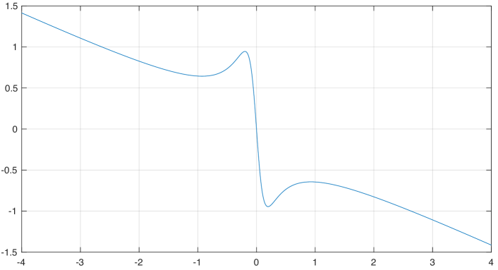
Figure 1: Graph of the function $\phi(\hat{x})=-{(\hat{x}+\hat{x}^{3})}/{(0.1+3\hat{x}^{2})}$. The positive slope around $\hat{x}=\pm\tfrac{1}{2}$ implies that the system $\dot{\hat{x}}=\phi(\hat{x})$ is not contracting with respect to a constant metric. However, it is in the set CT2.

IV Learning from Data

Within a set of stable observers, it is natural to try to find the one that is “best” in some sense. A standard way to formulate the problem is to specify a particular stochastic model of the true system, e.g. in the DT case

$$x_{t+1}=a(x_{t},u_{t},w_{t}),\quad y=g(x_{t},u_{t},w_{t})$$ (27)

where $u_{t}$ is a known input, and $w_{t}$ represents measurement and/or process noise, and is unknown but drawn from a known probability distribution (we assume $w=0$ corresponds to a “nominal” model). Initial conditions may be known, or also drawn from a probability distribution. Then a measure of state estimation error is chosen, e.g. the mean-square error:

$$J=\lim_{T\rightarrow\infty}\frac{1}{T}\sum_{t=0}^{T}\mathcal{E}[(x_{t}-\hat{x}_{t})^{\prime}(x_{t}-\hat{x}_{t})],$$

where $\mathcal{E}$ denotes the expectation operator (see, e.g., [1]). Unfortunately there is no computationally tractable solution to this problem for most nonlinear systems, so some form of approximation is required.

We propose an approach based on “learning from data”. The procedure we propose is outlined as follows:

1. Construct a “flexible” set of contracting nonlinear observers for the nominal ($w=0$) model.

2. Draw one or more realisations of $w$ and simulate the stochastic model (27), collecting data sets $\tilde{z}=\{\tilde{x}_{t},\tilde{u}_{t},\tilde{y}_{t}|t=0,1,...,T\}$ as the realisations of $x,u,y$.

3. Optimize over the set of observers for one which minimizes the empirical mean-square error:

   $$J=\frac{1}{T}\sum_{t=0}^{T}|\hat{x}_{t}-\tilde{x}_{t}|^{2}$$

   where $\hat{x}$ are solutions of the observer simulated with data $\tilde{u}_{t},\tilde{y}_{t}$, and an estimate of $\hat{x}_{0}$. When multiple realisations of $w$ are sampled, $J$ is the sum of the corresponding mean-square errors.

If a method is available for simulating a stochastic CT model, then the same approach can be applied to optimize sampled-data observers by subsampling at fixed rate.

Remark 2

In the linear case, the constraint that the learned observer is an observer for the nominal system means the resulting estimator is unbiased when $w$ is zero mean. In the nonlinear case this is not generally true, but it can be considered as a form of regularization that introduces a bias to ensure reliable behaviour on data not in the training set.

While the above recipe can be followed using generic nonlinear programming methods to minimize $J$, this may prove challenging since $J$ is a highly non-convex function of the observer parameters even in the linear case. We construct a convex approximation based on Lagrangian relaxation of linearized estimation error, similar to the method proposed in [28] for system identification.

First we construct the linearization along the sampled “true solution” $\tilde{x}$, by introducing the local deviation $\tilde{\Delta}_{t}\approx\hat{x}_{t}-\tilde{x}_{t}$ obeying the dynamics

$$E(\tilde{x}_{t+1})\Delta_{t+1}=F(\tilde{x}_{t},\tilde{u}_{t})\tilde{\Delta}_{t}+\epsilon_{t}.$$ (28)

with $\tilde{\Delta}_{0}=0$, where the equation errors $\epsilon_{t}$ are defined as

$$\epsilon_{t}:=e(\tilde{x}_{t+1},u_{t+1},y_{t+1})-f(\tilde{x}_{t},\tilde{u}_{t},\tilde{y}_{t})$$

Then the local mean-square error is

$$J^{0}(\theta,\tilde{z})=\frac{1}{T}\sum_{t=0}^{T}|\Delta_{t}|^{2},$$ (29)

Roughly speaking, when the state estimation error is small, i.e. $\tilde{\Delta}_{t}\approx\hat{x}_{t}-\tilde{x}_{t}$ then $J\approx J^{0}$. A more formal derivation for system identification problems can be found in [28, Sec. V.B]. Note that if the observer dynamics are affine in $\hat{x}$, then $J$ and $J^{0}$ are identical.

The problem of minimizing $J^{0}$ remains nonconvex, but a semidefinite programming bound can be constructed using Lagrangian relaxation [28]. This is most clearly expressed be rewriting (28) in a “lifted” representation

$$H(\theta,\tilde{z})\vec{\Delta}=\vec{\epsilon}(\theta,\tilde{z})$$

with the stacked vectors $\vec{\Delta}:=[\tilde{\Delta}_{1}^{\prime},\tilde{\Delta}_{2}^{\prime},...,\tilde{\Delta}_{T}^{\prime}]^{\prime}$ and $\vec{\epsilon}(\theta,\tilde{z}):=[\epsilon_{0}^{\prime},\epsilon_{1}^{\prime},...\epsilon_{T}^{\prime}]^{\prime}$ and $H(\theta,\tilde{z})$ is a block lower-bidiagonal matrix that is affine in $\theta$ and is straightforward to construct from (28).

Then a convex upper bound for $J^{0}$ is given by

$$\hat{J}^{0}(\theta,\tilde{z}):=\sup_{\vec{\Delta}\in l_{T}^{nT}} \{|\vec{\Delta}|^{2}-2\vec{\Delta}^{\prime}(H(\theta,\tilde{z})\vec{\Delta}-\vec{\epsilon}(\theta,\tilde{z}))\}.$$

It can be shown that for all systems satisfying the contraction constraint, the supremum over $\vec{\Delta}$ is finite, and can be written in explicit form:

$$\hat{J}^{0}(\theta,\tilde{z})=\vec{\epsilon}(\theta,\tilde{z})^{\prime}\mathcal{H}(\theta,z)^{-1}\vec{\epsilon}(\theta,\tilde{z})$$ (30)

where $\mathcal{H}=H+H^{\prime}-I$ or, via Schur complement, in the equivalent semidefinite programming representation:

$$\hat{J}^{0}(\theta,\tilde{z})=\min s\quad\textrm{ s.t. }\begin{bmatrix}s&\vec{\epsilon}(\theta,\tilde{z})^{\prime}\\ \vec{\epsilon}(\theta,\tilde{z})&\mathcal{H}(\theta,z)\end{bmatrix}\geq 0.$$ (31)

Algorithms have been developed for efficient solution of problems with this structure [31, 32]. Both have computational complexity that is linear in the data length $T$, rather than cubic for a generic semidefinite programming solver.

The main result regarding $\hat{J}^{0}$ is the following:

Theorem 5

For all $P=P^{\prime}>0$ and signal data $\tilde{z}$, for every $\theta\in\Theta$, $J^{0}(\theta,\tilde{z})\leq\hat{J}^{0}(\theta,\tilde{z})<\infty.$ Furthermore, if the data set $\tilde{z}$ is generated with $w=0$, then the optimal values satisfy $J^{0,\star}(\tilde{z})=\hat{J}^{0,\star}(\tilde{z})=0.$

We omit the details of the proof because of space restrictions, since it is similar to [28, Theorem 6].

V Examples and Discussion

In this section we illustrate the method with some numerical simulations. The first example system we consider was previously studied in [12]:

$$\dot{x}=a(x)=\begin{bmatrix}x_{2}\\ x_{2}-\frac{1}{3}x_{2}^{3}-x_{2}x_{3}^{2}\\ x_{2}-x_{3}-\frac{1}{3}x_{3}^{3}-x_{3}x_{2}^{2}\end{bmatrix},\quad y=g(x)=x_{1}$$

The solution given in [12] relied on a certain ingenuity on the part of the designer, recognising the system can be decomposed into a linear part and a monotonic nonlinearity. In comparison, our method is quite “plug and play”: we apply Theorem 1 using CT1 as a contracting set and $f$ the set of degree-three polynomials in $\hat{x},y$, the contraction constraint is imposed via sum-of-squares [15], and an observer is found in 1.41 seconds on 3.1 GHz Intel Core i7 with 16GB RAM.

A bisection search over $\lambda$ reveals that $\lambda=1$ is the best rate of exponential convergence in this observer set, and with $\lambda=1$ we computed the observer that minimized the $\ell^{1}$ norm of the coefficients of $f$, to encourage sparsity of coefficients. All computations were done using Yalmip [33] and Mosek.

Fig. 2 shows the evolution of the three states (solid lines) from initial conditions $x_{0}=[-3,4,1]^{\prime}$ and the observer states (dashed lines) initialized at $\hat{x}_{0}=[0,0,0]^{\prime}$. Also shown are the states of the sampled-data observer (circles) proposed in Section III-C with a sampling interval $h=0.1s$. It can be seen that the sampled-data observer is a good approximation to the CT observer, and converges rapidly to the true states.

In Fig. 3 we show corresponding results with a longer sampling interval of $h=0.3s$. It can now be seen that the behaviour of the CT and sampled-data observers are quite different in the initial transient, nevertheless both converge to the true states.

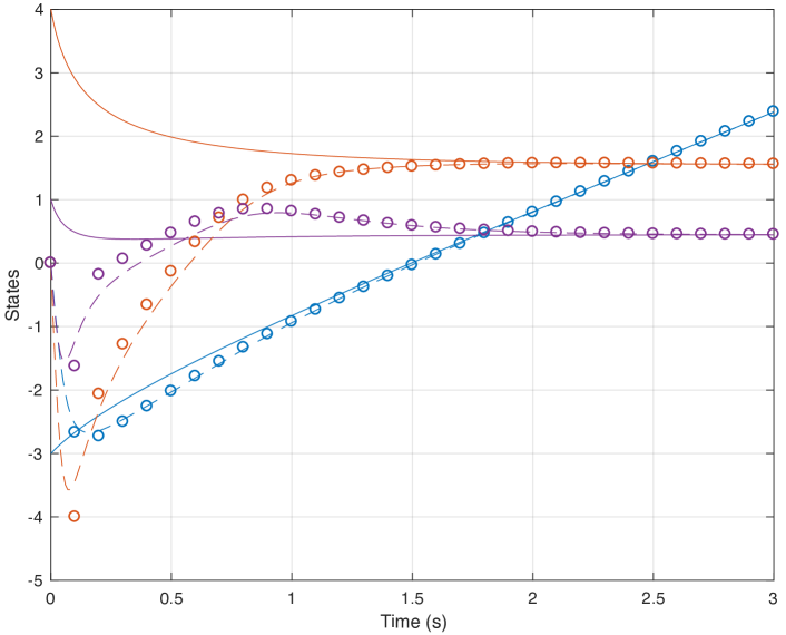
Figure 2: Comparison of true states (solid lines), CT observer (dashed lines), and sampled-data observer (circles) with sampling interval $h=0.1s$.

We next tested the ability of the learning approach in Section IV to find an observer with good performance on noisy data. To generate training data we simulated the CT system over 5 seconds, sampled the state $\tilde{x}$ and output with sampling interval $h=0.1s$, added Gaussian white noise of variance 0.01 to the output to generate $\tilde{y}$, and then minimized $\hat{J}^{0}$ over the set CT1 with $H=10^{-8}I$.

We tested the resulting observer against the previously-designed observer (optimal with respect to $\lambda$) on 50 realisations of validation data, generated in the same way. A boxplot of the resulting mean-square errors is shown in Fig. 4. For this example, the learned observer has around half the median error and one third the worst-case error of the observer optimized for $\lambda$.

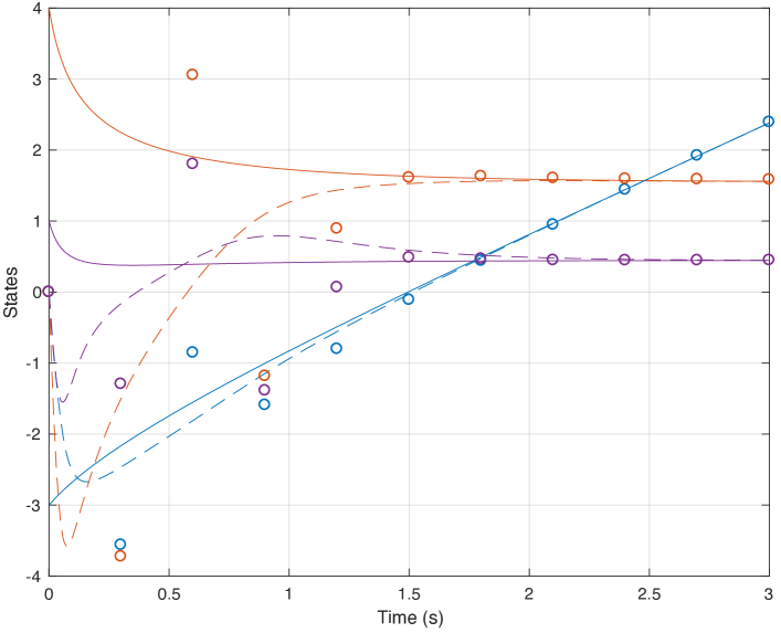
Figure 3: Comparison of true states (solid lines), CT observer (dashed lines), and sampled-data observer (circles) with sampling interval $h=0.3s$.

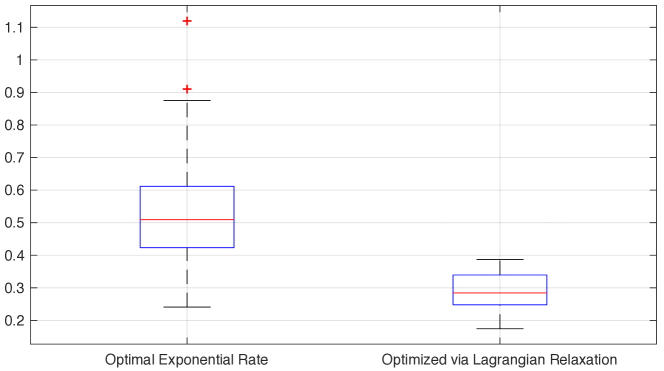
Figure 4: State estimation error on noisy validation data, comparing the observer which is optimal in terms of exponential rate to the one which is optimized for noise performance via Lagrangian relaxation.

To benchmark the proposed learning method against a “gold standard”, we now turn to observer design for linear discrete-time systems and compare to the Kalman filter. We compare performance on randomly sampled systems, using different amounts of training data, as follows:

1. For each data length $T\in\{100,250,500,1000,2000\}$ do the following

2. Sample 20 random 4th-order systems using Matlab drss command, eliminating systems with pure integrators. For each system compute the steady-state Kalman filter and do the following:

3. Generate a random training data set of length $T$ and train a DT observer using the method of Sec. IV.

4. Sample 25 random validation data sets of length and compute the relative error for each, defined as a percentage:

   $$J_{rel}=100\tfrac{\sum_{t=0}^{T}|\hat{x}^{o}_{t}-\tilde{x}_{t}|^{2}-\sum_{t=0}^{T}|\hat{x}^{o}_{t}-\tilde{x}_{t}|^{2}}{\sum_{t=0}^{T}|\hat{x}^{k}_{t}-\tilde{x}_{t}|^{2}}$$

   where $\hat{x}^{o}$ is the state estimate from our learned observer, and $\hat{x}^{k}$ is the state estimate from the Kalman filter.

Boxplots of the computed $J_{rel}$ for all realisations are shown in Fig. 5, and the median values of $J_{rel}$ for each training-data length are collected in Table I. It can be seen that with just a few hundred training samples, the performance of the learned estimator comes within around 2% of the Kalman filter, and on some data sets outperforms the Kalman filter, indicated by negative quantities in Fig 5.

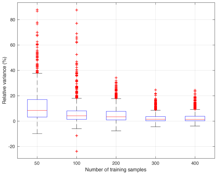
Figure 5: Comparison to the Kalman filter: boxplot of $J_{rel}$ vs number of samples used for training

TABLE I: Medians of $J_{rel}$ for each training-data length

Samples (N)	50	100	200	300	400
Median $J_{rel}$ (%)	8.4336	4.2223	3.4214	1.4955	1.3731

VI Conclusions

In this paper, we have introduced methods for constructing convex sets of contracting CT, DT, and sampled-data observers for a given nonlinear system. We propose optimizing over these sets to based on sampled simulation data to “learn” and observer with good performance on noisy data.

While we have focused on the case that the observer state is $\hat{x}$, the proposed methods can be adapted to reduced-order and excessive-order observers. Also important is the case of “reduced-complexity” nonlinear observers, for which the correctness condition is infeasible, i.e. when the true system dynamics are not in the span of (12), one can relax correctness to bounded error in (8) subsets of $\mathbb{R}^{n}\times\mathbb{R}^{m}$. Investigation of these approaches is underway.

References

- [1] B. D. O. Anderson and J. B. Moore, Optimal Filtering. Prentice Hall, 1979.
- [2] I. R. Petersen and A. V. Savkin, Robust Kalman Filtering for Signals and Systems with Large Uncertainties. Springer Science & Business Media, 1999.
- [3] A. Doucet, N. De Freitas, and N. Gordon, Sequential Monte Carlo Methods in Practice. Springer Verlag, 2001.
- [4] C. V. Rao, J. B. Rawlings, and D. Q. Mayne, “Constrained state estimation for nonlinear discrete-time systems: Stability and moving horizon approximations,” IEEE transactions on automatic control, vol. 48, no. 2, pp. 246–258, 2003.
- [5] J. S. Shamma and K.-Y. Tu, “Approximate set-valued observers for nonlinear systems,” IEEE Transactions on Automatic Control, vol. 42, no. 5, pp. 648–658, May 1997.
- [6] L. Praly, “Observers for Nonlinear Systems,” Encyclopedia of Systems and Control, pp. 935–943, 2015.
- [7] A. J. Krener and A. Isidori, “Linearization by output injection and nonlinear observers,” Systems & Control Letters, vol. 3, no. 1, pp. 47–52, Jun. 1983.
- [8] H. K. Khalil and L. Praly, “High-gain observers in nonlinear feedback control,” International Journal of Robust and Nonlinear Control, vol. 24, no. 6, pp. 993–1015, Apr. 2014.
- [9] D. Karagiannis, D. Carnevale, and A. Astolfi, “Invariant Manifold Based Reduced-Order Observer Design for Nonlinear Systems,” IEEE Transactions on Automatic Control, vol. 53, no. 11, pp. 2602–2614, Dec. 2008.
- [10] V. Andrieu and L. Praly, “On the Existence of a Kazantzis–Kravaris/Luenberger Observer,” SIAM Journal on Control and Optimization, vol. 45, no. 2, pp. 432–456, Jan. 2006.
- [11] M. Arcak and P. Kokotović, “Nonlinear observers: A circle criterion design and robustness analysis,” Automatica, vol. 37, no. 12, pp. 1923–1930, Dec. 2001.
- [12] X. Fan and M. Arcak, “Observer design for systems with multivariable monotone nonlinearities,” Systems & Control Letters, vol. 50, no. 4, pp. 319–330, Nov. 2003.
- [13] D. Coutinho, C. de Souza, K. Barbosa, and A. Trofino, “Robust Linear $H_{infty}$ Filter Design for a Class of Uncertain Nonlinear Systems: An LMI Approach,” SIAM Journal on Control and Optimization, vol. 48, no. 3, pp. 1452–1472, Jan. 2009.
- [14] C. Ebenbauer, J. Renz, and F. Allgower, “Polynomial Feedback and Observer Design using Nonquadratic Lyapunov Functions,” in Proceedings of the 44th IEEE Conference on Decision and Control, Dec. 2005, pp. 7587–7592.
- [15] P. A. Parrilo, “Semidefinite programming relaxations for semialgebraic problems,” Mathematical Programming, vol. 96, no. 2, pp. 293–320, 2003.
- [16] W. Lohmiller and J.-J. E. Slotine, “On Contraction Analysis for Non-linear Systems,” Automatica, vol. 34, no. 6, pp. 683–696, Jun. 1998.
- [17] R. Sanfelice and L. Praly, “Convergence of Nonlinear Observers on With a Riemannian Metric (Part I),” IEEE Transactions on Automatic Control, vol. 57, no. 7, pp. 1709–1722, Jul. 2012, 00014.
- [18] A. P. Dani, S. J. Chung, and S. Hutchinson, “Observer Design for Stochastic Nonlinear Systems via Contraction-Based Incremental Stability,” IEEE Transactions on Automatic Control, vol. 60, no. 3, pp. 700–714, Mar. 2015.
- [19] D. Lewis, “Metric properties of differential equations,” American Journal of Mathematics, pp. 294–312, 1949.
- [20] F. Forni and R. Sepulchre, “A Differential Lyapunov Framework for Contraction Analysis,” Automatic Control, IEEE Transactions on, vol. 59, no. 3, pp. 614–628, 2014.
- [21] I. R. Manchester and J.-J. E. Slotine, “Transverse Contraction criteria for existence, stability, and robustness of a limit cycle,” Systems & Control Letters, vol. 62, pp. 32–38, 2013.
- [22] I. R. Manchester and J. J. E. Slotine, “Control Contraction Metrics: Convex and Intrinsic Criteria for Nonlinear Feedback Design,” IEEE Transactions on Automatic Control, vol. 62, no. 6, pp. 3046–3053, Jun. 2017.
- [23] M. Arcak and D. Nešić, “A framework for nonlinear sampled-data observer design via approximate discrete-time models and emulation,” Automatica, vol. 40, no. 11, pp. 1931–1938, Nov. 2004.
- [24] J. Sjöberg, Q. Zhang, L. Ljung, A. Benveniste, B. Delyon, P.-Y. Glorennec, H. Hjalmarsson, and A. Juditsky, “Nonlinear black-box modeling in system identification: A unified overview,” Automatica, vol. 31, no. 12, pp. 1691–1724, 1995.
- [25] L. Ljung, System Identification: Theory for the User, 3rd ed. Englewood Cliffs, New Jersey, USA: Prentice Hall, 1999.
- [26] R. Pascanu, T. Mikolov, and Y. Bengio, “On the difficulty of training recurrent neural networks,” in International Conference on Machine Learning, 2013, pp. 1310–1318.
- [27] M. M. Tobenkin, I. R. Manchester, J. Wang, A. Megretski, and R. Tedrake, “Convex optimization in identification of stable non-linear state space models,” in 49th IEEE Conference on Decision and Control (CDC). IEEE, 2010.
- [28] M. M. Tobenkin, I. R. Manchester, and A. Megretski, “Convex Parameterizations and Fidelity Bounds for Nonlinear Identification and Reduced-Order Modelling,” IEEE Transactions on Automatic Control, vol. 62, no. 7, pp. 3679–3686, Jul. 2017.
- [29] W. Wang and J.-J. E. Slotine, “On partial contraction analysis for coupled nonlinear oscillators,” Biological Cybernetics, vol. 92, no. 1, pp. 38–53, Dec. 2004.
- [30] G. G. Dahlquist, “A special stability problem for linear multistep methods,” BIT Numerical Mathematics, vol. 3, no. 1, pp. 27–43, Mar. 1963.
- [31] J. Umenberger and I. R. Manchester, “Specialized Algorithm for Identification of Stable Linear Systems using Lagrangian Relaxation,” in Proc. 2016 American Control Conference, Boston, MA, 2016.
- [32] M. S. Andersen, J. Dahl, and L. Vandenberghe, “Implementation of nonsymmetric interior-point methods for linear optimization over sparse matrix cones,” Mathematical Programming Computation, vol. 2, no. 3-4, pp. 167–201, Dec. 2010.
- [33] J. Lofberg, “Yalmip : A toolbox for modeling and optimization in MATLAB,” in Proceedings of the CACSD Conference, Taipei, Taiwan, 2004.