Dynamics of Embedded Curves by Doubly-Nonlocal Reaction-Diffusion Systems
Abstract
We study a class of nonlocal, energy-driven dynamical models that govern the motion of closed, embedded curves from both an energetic and dynamical perspective. Our energetic results provide a variety of ways to understand physically motivated energetic models in terms of more classical, combinatorial measures of complexity for embedded curves. This line of investigation culminates in a family of complexity bounds that relate a rather broad class of models to a generalized, or weighted, variant of the crossing number. Our dynamic results include global well-posedness of the associated partial differential equations, regularity of equilibria for these flows as well as a more detailed investigation of dynamics near such equilibria. Finally, we explore a few global dynamical properties of these models numerically.
1 Introduction
In a variety of physical and mathematical contexts, a curvature-regularized nonlocal interaction energy
| (1) |
governs the motion of a closed, embedded curve. For example, worm-like chain (WLC) models for DNA dynamics incorporate the bending energy (i.e. the squared curvature ) and an energetic barrier to self-intersection (i.e. a repulsive kernel ) that prevents topological changes. Dynamical models of protein folding [1] and vortex filaments [2] also take a similar form. At the purely mathematical end of the spectrum, a relatively recent trend in geometric knot theory has witnessed a growth in the energetic study of (1) and its variants [3, 4, 5, 6, 7]. A significant portion of this general line of work focuses on extremal properties of these various knot energies such as the existence, complexity and regularity of extremal embeddings within a given class of curves. In the context of (1), the bi-variate kernel encodes the interaction between pairs of points on a curve according to the principles of physical potential theory — an attraction or repulsion between points generically occurs in regions where increases or decreases in its first argument, respectively. A typical kernel will exhibit a singular, short-range repulsion and possibly an additional regular, far-field attraction, yet even this reasonable level of generality in the choice of kernel leads to a class of models that exhibit a striking variety of complex and intricate dynamics.
We study the energetics and dynamics of (1) from both an analytical and a numerical perspective. At an energetic level, we establish a set of inequalities that relate the nonlocal energy (1) to classical, combinatorial measures of complexity for embedded curves. These results prove similar, in spirit, to a variety of work on “knot energies” that emanates from the knot theory community [8, 9, 10, 11, 12, 13]. Our arguments reveal the sense in which some combinatorial measures of complexity, such as the average crossing number, have fractional Sobolev spaces, lurking just underneath the surface. This insight allows us to establish complexity bounds for a rather broad class of kernels and it also provides the impetus to introduce generalizations of such complexity measures. In this sense, our work complements that strand of geometric knot theory that emphasizes the importance of taking a more analytic approach to (1) and its variants [14, 15, 16]. For instance, the relative importance of harmonic analysis vis-à-vis Möbius invariance has been observed when studying regularity of extremal embeddings [17]. At a dynamic level, we study a corresponding “constrained gradient flow” of the energy (1) that restricts the dynamics to lie in the class of unit speed parameterizations. This is a slightly non-standard approach since we do not simply functionally differentiate (1) with respect to , but it leads to an analytically and numerically well-behaved dynamical model. In particular, enforcing a uniform density along at each time yields semi-linear rather than quasi-linear dynamics and also gives uniform numerical samples along at each numerical time-step without having to resort to re-parameterizations. At a physical level, we may view our choice of dynamics as a hard limit of WLC models that include energetic barriers to bond stretching, in the sense that an infinite barrier to bond stretching results from constraining the flow to lie in the class of unit speed curves. This approach to dynamics leads to a class of nonlocal reaction-diffusion systems driven by doubly-nonlocal forcings. The pairwise interaction energy leads to a forcing whose derivative along satisfies
and so recovering from requires two consecutive nonlocal operations. We refer to the resulting class of dynamics as a doubly-nonlocal reaction-diffusion system to emphasize this structure. Overall, this approach to dynamics allows us to obtain a global well-posedness result under quite general hypotheses on to demonstrate regularity of critical embeddings, to perform a detailed study of equilibria and to devise reliable numerical procedures.
Most of our arguments rely, at least in part, on some basic harmonic analysis and a few notions from knot theory; we begin by reviewing this material in the next section. We then proceed to study the energy (1) from a complexity point-of-view in the third section. As an example in this direction, a corollary of our analysis shows that the distortion and bending energy bound the average crossing number
| (2) |
of an embedding. An analogous result holds for (1) provided satisfies a “homogeneity” assumption. This is perhaps surprising in light of the following observation: There exists an infinite sequence of ambient isotopy classes of knots with uniformly bounded distortion as well as an infinite sequence of ambient isotopy classes of knots with uniformly bounded bending energy. These sequences therefore exhibit “conflicting” behavior, since (2) rules out the existence of such an infinite sequence when both distortion and bending energy remain uniformly bounded. We also show that an energy of the form (1) induces, in a quantified sense, a stronger invariant than the average crossing number. These results are motivated by analogous results for the Möbius energy [11] (i.e. (1) with and without curvature) and the ropelength [13, 18, 19, 20, 21]; however, our results are not entirely comparable with these earlier works and we generally prove them using different means. We then proceed to address the dynamics of (1) in the fourth section. We initiate this process by proving global well-posedness and regularity under certain “homogeneity” and “degeneracy” assumptions on the kernel . These assumptions cover many of the kernels that have generated prior interest in the literature [22, 23, 24, 25], and the main contribution here lies in finding a relatively general and broadly applicable hypothesis under which such a global result holds. This result complements prior work that proves global existence for (1) under the Möbius kernel [3], although we assign dynamics in a slightly different fashion. We conclude the fourth section with an analysis of dynamics near equilibrium. For instance, it is known that unit circles globally minimize (1) under proper monotonicity and convexity assumptions [26], and in addition, that desirable regularity properties (e.g. smoothness) hold for critical points of the O’Hara and Möbius energies [15, 17]. We supplement this by adapting techniques for nonlocal dynamical systems to show that circles are also properly “isolated” modulo to rotation and scaling invariance. This yields a local asymptotic stability result for our dynamics, which should be compared to [27] and the recent contribution [7] for the special case of pure Möbius flow. We use a similar technique to show that the natural “global” version of this result fails for a pure bending energy flow: There exist unknotted initial configurations that remain unknotted for all time under a bending energy flow, yet the dynamics do not asymptotically converge to the globally minimal, unknotted circle. This dynamic result complements the energetic result, proved in [28], that the double-covered circle the unique bending energy minimizer for the trefoil knot type. Finally, we explore global dynamical properties numerically in the final section.
To place these efforts in context, note that a large body of work has studied the energetics and dynamics of various knot energies. Much of the work in the field has focused on a few families of knot energies such as those suggested in [4], including tangent-point energies [29, 14], Menger curvature energies [5] and O’Hara’s energies [22, 23, 24, 25] (of which the Möbius energy [11] is a special case). The most closely related examples include work on the energetics and minimizers of integral Menger curvature [16] , as well as work on the energetics and criticality theory for the Möbius energy [7, 11, 17, 27] and the extended O’Hara family [6, 15] . In contrast to these energies, the physical model (1) crucially depends on the bending energy which, as previously noted [3], obviously improves the analytic properties of the total energy. When taken together our results show that, in addition to its physical significance, the admission of the bending energy and a (quite weak) barrier to self-intersection in (1) allows for a wide class of models that exhibit all of the analytic features that have previously motivated knot energies.
2 Preliminary Material
We begin our study by introducing the notation we shall use, then providing a few key definitions and finally recording a series of preliminary lemmas on which we will rely throughout the remainder of the paper. Lightface roman letters such as and will denote real numbers; their boldface counterparts and will denote three-dimensional vectors. We reserve for the canonical standard basis. Given we use for the standard Euclidean inner-product, for the cross product and for the Euclidean norm. The notation denotes the scalar triple product. We use to denote the standard one-dimensional torus, which we view as the interval with endpoints identified. For we define
and then extend to all of via -periodicity. Thus for any pair of points the quantity simply gives the geodesic distance between them. Given a square-integrable function we shall always use the definition and notation
to denote the -norm, with the dimensionality omitted but always clear from context. We shall use
to denote the forward and inverse Fourier transforms, so that
provide the norm as above and an equivalent definition of the Sobolev norm. For any sufficiently regular mapping we use or to denote ordinary differentiation in both the strong and weak sense. We say a rectifiable has unit speed if on and we then set or simply as the pointwise curvature of such an embedding. Similarly, we say a rectifiable has constant speed if , where
denotes the length of the embedded curve. Conversely, given any tangent field with and we may define
and thereby recover a -periodic, constant speed curve that has and center of mass at the origin. We refer to as the knot induced by such a vector-field. Given mean zero function we analogously use
to denote its mean zero primitive.
In addition to these notations, we also need to recall a few elementary facts from harmonic analysis. First, for a given we use the notation
| (3) |
to denote its maximal function, see, for example, [30, p.216]. We then recall the standard fact that the map defines a bounded operator on , so that
| (4) |
for some absolute constant. If has unit speed then furnishes its pointwise curvature, in which case we define and refer to as the curvature maximal function. The following elementary lemma will also prove useful —
Lemma 2.1.
Assume that and that there exist finite constants so that the decay estimates
hold. Then the product obeys the decay estimate
for a universal constant. If obey the decay estimates
where are finite constants and are arbitrary exponents, then the product obeys the decay estimate
with a positive constant depending only upon the exponents.
See [31] lemma 6.1 and lemma 6.2, for instance, for an indication of the proof.
Recall that a unit speed embedding is bi-Lipschitz if there exists a constant so that the inequality
holds for any possible pair of points. Thus exactly when Gromov’s distortion
is finite, with furnishing the smallest possible bi-Lipschitz constant. Moreover, the lower bound holds for any closed, rectifiable curve with unit speed, see pp.6-9 [32]. We shall refer to any pair of points for which
as a distortion realizing pair. A simple invocation of Taylor’s theorem shows that
for any with unit speed, and thus any such actually admits a distortion realizing pair. Given a bi-Lipschitz embedding with unit speed, we define
| (5) |
as the maximal distance on between any distortion realizing pair. By applying the first derivative test to the expression we obtain
and so by applying Taylor’s theorem and the triangle inequality to bound the right hand side of this expression from below we obtain a lower bound
| (6) |
for the distance on between any such pair. Finally, if a bi-Lipschitz embedding has unit speed and if we define as
we may appeal to Taylor’s theorem one final time to conclude that the inequalities
| (7) |
hold. Despite their elementary proofs, these inequalities prove quite useful.
Finally, for given a bi-Lipschitz embedding we shall use to denote a generic ambient isotopy class. Similarly, we shall employ while the notation if we wish to emphasize the class induced by some underlying curve. The following lemma from [33] and the embedding shows that ambient isotopy classes are well-behaved with respect to convergence in both the and topologies —
Lemma 2.2.
Let denote a positive velocity, simple closed curve. Then there exists such that all satisfying are ambient isotopic. In particular, if is sufficiently small.
3 Basic Energetics
This section provides a brief analysis of nonlocal energies that, when defined over unit speed embeddings, take the form
| (8) |
for some bi-variate kernel. We shall also consider the normalized or scale-invariant bending energy
as well as the superposition of such nonlocal energies (8) with the bending energy. Well-known examples of kernels in (8) include
| (9) |
The motivation for these choices arises, at least in part, from the fact then defines a differentiable approximation of the distortion. More specifically, prior work [11, 24] demonstrates that necessarily implies that has finite distortion. Moreover, the O’Hara family converges as and to the log-distortion of after a suitable normalization. This observation suggests the somewhat more obvious family
since then corresponds to the classical -norm approximation of the -norm. Further motivations for using (9) include the fact that the Möbius energy and a large class of the O’Hara energies attain their global minimum at the standard embedding of the unit circle, as well as the fact that the Möbius energy exhibits a relationship with classical combinatorial quantities such as the crossing number.
We now show that a very large class of energies based on have these three motivating properties. In a certain sense these properties are best understood from a pure analytical point-of-view, rather than from an appeal to geometric or topological considerations (e.g. Möbius invariance). This point of emphasis echoes an observation made in earlier work on the Möbius energy — the smoothness of its critical points follows without explicitly appealing to Möbius invariance itself [17]. We begin by showing that, provided exhibits a sufficient degree of singularity, finiteness of the integral (8) necessarily implies that an curve is bi-Lipschitz. We shall also obtain a concrete bound for the distortion in terms of and the semi-norm in the process, although the bound itself is far from optimal for general kernels.
Lemma 3.1.
Assume that satisfies the homogeneity property
for some exponent and some function . Assume that the lower bound holds on as well. If has unit speed then
for finite constants. Moreover, if then
| (10) |
and so is bi-Lipschitz if is finite.
Proof.
See appendix, lemma 7.1 ∎
The homogeneity hypothesis provides a means to unify and simplify our analysis, yet it proves general enough to cover all families introduced so far. For instance, we have and for the Möbius energy, the relations and for the O’Hara family and and for the -distortion. The lemma therefore applies for all three families, provided in the second case and in the final case. It is also clear that the conclusion holds for kernels of the form with an homogeneous kernel and bounded from below, although we have no impetus to pursue this level of generality since the requisite modifications to the argument and its conclusion are straightforward. Finally, we cannot remove the dependence on or dispense with the hypothesis that and still have the conclusion of the lemma hold at this level of generality. Indeed, for the -distortion family it is easy to construct a smooth sequence for which remains uniformly bounded but and diverge.
The previous lemma illustrates the fact that a wide class of energies
approximate the distortion. Under similar hypotheses on the kernel both the energy and the bending energy attain their global minima at the standard embedding of the unit circle [26, 34]. We shall quickly review the arguments underlying these known facts, as this discussion will allow us to emphasize an analytical point — both arguments appeal to the same classical technique in the calculus of variations, i.e. the use of Poincarè-type inequalities with optimal constants. For instance, the statement follows directly from the Poincarè-type inequality
| (11) |
with optimal constant. Following [26], for unit speed curves the inequality (11) yields
whenever decreases in its first argument over the non-negative reals. By Jensen’s inequality this in turn shows that
whenever is also convex. Demonstrating global optimality of for the bending energy proceeds in a similar fashion. In this case the classical Poincarè inequality with optimal constant
| (12) |
provides the starting point. Letting denote the unit speed embedding of a simple appeal to parametrization and scale invariance of shows
As the class of standard circles furnish the only unit speed curves that achieve equality in either (11) or (12), we may recall
Theorem 3.2.
Suppose that for each the function is non-decreasing and convex on . Then for any the energy
attains its minimum over unit speed curves at the unit circle. Moreover, if either or is strictly decreasing then unit circles are the unique global minimizers.
In particular, the Möbius energy as well as the O’Hara family and the -Distortion family all have as their global minimizer. Once again, the arguments above leading to this theorem are both standard and known [11, 25, 26]; we recall them simply to emphasize the connection between them as well as the broader connection to classical PDE and variational arguments. Thus there are analytical properties, such as convexity and Sobolev inequalities, rather than geometric properties, such as Möbius invariance, lying at the heart of the matter.
Finally, we turn our attention toward relating the energies and to more classical measures of complexity. Once again, analytical considerations and Sobolev spaces shall come to the fore. A corollary of this analysis will also allow us to illustrate that an energy of the form induces, in a certain sense, a much stronger invariant than the crossing number. Following [11, 35, 36], we shall begin by considering the mapping defined by
with a Lipschitz embedding with finite distortion. For any such Lipschitz curve the function is Lipschitz in both variables whenever and has finite distortion. For such functions, the co-area formula for Lipschitz maps [37] therefore implies that
provided is a positive, Lebesgue measurable function. For a given let us define the crossing set as
where represents the corresponding planar curve induced by orthogonal projection. Thus precisely when distinct points of self-intersect. As the equality
holds by a trivial calculation, we may therefore conclude
| (13) |
When the integrand
in (13) simply gives the cardinality of and so (13) reduces to a constant multiple of the average crossing number. We may utilize the non-negative function to apply a positive weight applied to each point of self-intersection in and in this way arrive at a weighted generalization or “weighted” crossing number. By analogy with electrostatics, we shall consider the simple power-law family
| (14) |
of weighting functions, where denotes the arc-length between points. We may then view (13) as inducing a “repulsion” between points of self-intersection, in the sense that small values occur when weighted crossings are, on average, equally spaced along as measured by relative length. We primarily intend this family as an analytical device or gauge for measuring and drawing analytical comparsions — a bound on (13) for represents a stronger conclusion, in general, than a bound on the crossing number or average crossing number. Moreover, for smooth curves Taylor’s theorem immediately yields
while the denominator in (13) scales like near the origin. If we define as (13) with the weight (14) then a bound of the form
| (15) |
represents the strongest possible conclusion, and therefore the upper limit of our analytical scale.
We shall need with the following lemma in order to perform our analytical comparison.
Lemma 3.3.
Assume that and that has finite distortion. Assume further that has constant speed. Then
| (16) |
and if then the constant
is finite.
Proof.
See appendix, lemma 7.2 ∎
This lemma allows us to relate combinatorial measures of complexity for a curve to more standard measures of regularity of the embedding. By taking and evaluating the constant explicitly we may observe the most straightforward consequence, i.e. the inequality
| (17) |
for the average crossing number. To help place this inequality in a more familiar context, given an exponent and a rectifiable let us define the scale-invariant total -curvature of as
The case yields the (square root of) the bending energy, while the case reduces to Milnor’s notion of total curvature [10]. For constant speed curves and the inequality
holds, for some positive constant, due to the Hausdorff-Young inequality. If we may therefore conclude the following total -curvature bounds
| (18) |
for the average crossing number. From this observation we conclude that essentially any assumption whatsoever that is stronger than an assumption of finite total curvature yields a bound for the average crossing number. Indeed, instead of assuming for some we could also invoke the slightly weaker assumption that lies in the real Hardy space and still deduce an average crossing number bound. As the constants do not remain bounded, however, and so the natural “limiting” conclusion of (18) need not hold in general. The Hardy space usually serves as the substitute for in such a circumstance, but as (17) reveals, the fractional Sobolev space is actually the natural choice: The inequality (17) recovers the “proper” limiting inequality as , for while neither embedding
holds, the finiteness of implies the finiteness of both. As we recover the norm rather than finite total curvature in (17), and it is therefore the natural measure of regularity to use. It prefers oscillatory components in the curvature measure rather than the piecewise-constant curvature measures that characterize embeddings with finite total curvature, and so embeddings with oscillatory curvature rather than piecewise-linear embeddings must necessarily have finite average crossing number.
Another corollary of the bound (17) shows that finite bending energy and finite distortion imply a finite average crossing number. In fact we obtain a stronger conclusion from this analysis, in that an assumption of finite bending energy yields a significantly stronger conclusion than a simple crossing number bound. Specifically, for any the weighted crossing number
| (19) |
remains bounded whenever has finite distortion and finite bending energy. To appreciate the significance of this bound, recall that Gromov has provided an infinite sequence of ambient isotopy classes that have uniformly bounded distortion [38, p.308]. In addition, every -torus knot has a smooth unit-length embedding in such that for every [28], and so there also exists an infinite sequence of ambient isotopy classes with uniformly bounded bending energy. The crossing number bounds the weighted crossing number from below and defines a finite-to-one invariant (i.e. for every fixed integer there are at most finitely many knots with crossing number equal to ), so (19) cannot hold if we neglect either the bending energy or the distortion. However, by combining them we obtain not only a crossing number bound, but in fact a stronger weighted crossing number bound. Moreover, (19) shows that no infinite sequence of embeddings of distinct ambient isotopy classes of knots has both uniformly bounded distortion and uniformly bounded bending energy. A similar bound applies for whenever the kernel satisfies lemma 3.1, and so the energy is stronger than the weighted crossing number in an analogous sense.
Finally, it is worth briefly mentioning the consequences of (19) at the level of invariants. We may use or the weighted crossing number to define invariants via minimization in the standard way, i.e. by defining
for an arbitrary ambient isotopy class. That (under appropriate hypotheses on the kernel) and actually attain their minima within an ambient isotopy class follows from lemma 2.2 and a standard argument based on the direct method. For these invariants a bound of the form
holds for arbitrary. By appealing to results relating the curvature and distortion to ropelength [18, 19, 20, 21] and ropelength to crossing number [12] we may also conclude the corresponding upper bound
and so these invariants are polynomially equivalent.
4 Dynamics of Embedded Curves
With a basic understanding of the energies established, we now turn our attention toward the dynamics they induce via the constrained gradient flow
| (20) |
of such an energy. Given a bi-variate kernel we shall use
| (21) |
to denote the self-repulsive nonlocal forcing. For any tangent field defining the Lagrange multipliers and as
completes the description of the flow. The presence of these multipliers guarantees that and for all provided these properties hold initially. The corresponding induced knot
then defines a closed, constant speed curve for as long as the solution to (20) exists.
4.1 Local Existence
We first provide a local-in-time existence and uniqueness result for (20), which follows from a standard fixed-point argument. This argument requires a few minor but essential modifications to handle the technicality that, in general, our estimates for the nonlocal forcing (4) only apply when given a-priori a unit speed curve. Moreover, some classical existence results (e.g. [39]) cannot account for the presence of Lagrange multipliers as lower-order terms while still yielding the full strength of an existence result for generic initial data. Even so, the majority of this sub-section still qualifies as grunt work; the disinterested reader may comfortably skip the proofs and simply take the results for granted.
Our argument proceeds by establishing bounds and Lipschitz estimates on the lower-order terms in (20), and then proceeds to the existence proof itself. We begin with bounds for the nonlocal forcing (4), where for a given tangent field we shall always use to denote the induced knot. The process of obtaining these estimates will reveal those conditions on the kernel that our local existence approach requires. We shall make these requirements precise during the course of our arguments. To begin the task at hand, we recall the following basic result —
Lemma 4.1.
If and then the linear operator
| (22) |
defines an function. As a Fourier multiplier it acts as a (negative) fractional Laplacian
and in particular the operator-norm estimate
holds.
Proof.
See appendix, lemma 7.3 ∎
With this lemma in hand, we may establish the requisite estimates for by appealing to the following pair of lemmas. The first provides uniform bounds for the nonlocal forcing; the second provides a simple Lipschitz estimate. We shall only require that the interaction kernel satisfies some form of smoothness, homogeneity and cancelation or degeneracy condition in the course of obtaining these estimates. More specifically, we consider kernels obeying
-
(/ Homogeneity): There exists a function and an exponent so that
-
(0-Degeneracy): The function is and .
-
(-Degeneracy): For some non-negative integer the function is and has a root of order at
To motivate these definitions, we may observe that kernel
for the Distortion satisfies the homogeneity hypothesis with and thus -degeneracy applies to this family of examples. Similarly, the kernels
defining the O’Hara family satisfy homogeneity with and If and is sufficiently large, say and , then the kernel is also degenerate. These hypotheses therefore codify the sense in which both families provide distorion approximations (i.e. homogeneity) while still yielding convergent integrals for the corresponding energy (i.e. degeneracy). Under these hypotheses, we have
Lemma 4.2.
Assume that is homogeneous and either -degenerate or -degenerate. Assume that is a unit speed, bi-Lipschitz embedding. Then for the function
has mean zero. Moreover, obeys a uniform bound
for an -independent constant.
Proof.
See appendix, lemma 7.4 ∎
A simple reformulation of the argument underlying the lemma shows that
and so the principal value integral
exists in and obeys the same bound established in the lemma. Note also that the mean-zero property
continues to hold for the limit as well. With this issue under control, we may now proceed to establish a simple Lipschitz estimate on the principal value that will prove useful throughout our analysis. By imposing the hypotheses of lemma 4.2, we may also conclude
Lemma 4.3.
Assume that is homogeneous and either -degenerate or -degenerate. Let denote unit speed, bi-Lipschitz embeddings. Then for the uniform Lipschitz estimates
hold, where denotes an -independent constant.
Proof.
See appendix, lemma 7.5 ∎
As before, this lemma allows us to conclude that the principal value integrals obey the same Lipschitz estimate
as well. We then simply note that the nonlocal forcing
defines a continuous, periodic, function with mean zero. We may therefore infer that the estimates
| (23) |
hold for the nonlocal forcing in the gradient flow. We may finally complete the task at hand by establishing analogous bounds on the Lagrange multipliers
in the constrained flow. While these estimates follow from completely routine arguments, we provide proofs for the sake of completeness and concreteness. We begin by establishing that is non-singular and depends in a continuous fashion upon its input. Specifically, we have
Lemma 4.4.
Suppose that and that
for a positive constant. If is non-constant then
is non-singular. The operator norm estimate
also holds, and so exists and obeys
whenever is sufficiently small.
Proof.
See appendix, lemma 7.6 ∎
In our next lemma we establish the needed estimates on the Lagrange multipliers themselves.
Lemma 4.5.
Let denote arbitrary functions. Suppose and that
for a positive constant. Define
and then let
denote the corresponding Lagrange multipliers. Then the Lagrange multiplier bounds
| (24) |
and the Lipschitz estimates
| (25) |
hold whenever both and are non-singular. The constant is a multi-linear function of the quantities
alone, while the constant is a multi-linear function of the quantities
alone.
Proof.
Each inequality follows easily from the embedding and simple estimates of commutators via the triangle inequality. ∎
A straightforward combination of lemmas 4.2,4.3,4.4 and 4.5 is thankfully all we need, so our estimation task is complete.
With these estimates in hand, we may now proceed with a demonstration of local existence and uniqueness. We begin by working with the class of mild solutions to the evolution. We first set
as the lower-order contribution to (20), and use the more compact notation
to refer to the evolution equation. Following chapter 9 of [40], given an initial datum we then say that a continuous -valued function defines a mild solution to (20) on if
For a given the notation refers to the action of the linear semi-group generated by the heat equation on as usual it acts according to
where denotes the periodic heat kernel. We shall need the following proposition to get off the ground.
Proposition 4.6.
Suppose for arbitrary. Then for any initial datum the linear initial value problem
| (26) |
has a unique mild solution . For any the solution obeys the estimate
for a universal constant.
Proof.
See appendix, proposition 7.7 ∎
By linearity, this proposition obviously affords us a simple stability estimate
| (27) |
between distinct solutions as well. With this proposition in hand, we may proceed to establish a second intermediate result. It will allow us to apply a fixed-point argument in the class of mean zero, unit speed embeddings. This proposition is the main ingredient needed to prove local well-posedness. Throughout the remainder of this sub-section we use denote the -ball around in the norm.
Proposition 4.7.
Let for arbitrary. Suppose that on and define Lagrange multipliers according to
Let denote any initial datum with and unit speed. Then for any there exists a time depending only on and so that the initial value problem
has a unique mild solution with mean zero and unit speed.
Proof.
As has unit speed and mean zero, it is necessarily non-constant. Thus exists by lemma 4.4, and moreover the properties
hold for all provided is sufficiently small. By lemma 4.4, the choice of depends only on and . Fix such a , and given a time parameter let
For consider the mapping defined by
with denoting the lower-order terms. Lemma 4.5 implies that the estimates
hold whenever and are arbitrary. The constant depends only on and . By proposition 4.6 (more specifically (27)), if and then
The semigroup also satisfies
provided is sufficiently small, with the choice of depending only upon and itself. Thus provided is sufficiently small. For any such , if then proposition 4.6 (more specifically (27)) also yields
The mapping therefore defines a contraction on by taking smaller if necessary. For some sufficiently small, the equation
therefore has a unique mild solution . Moreover, and therefore the choice of depends only upon and as claimed.
The remainder of the proof is devoted to showing that has mean zero and unit speed. Fix as the existence interval and for let
denote the Fourier coefficient of the solution. Similarly, let
denote the Fourier coefficient of the lower-order terms in the evolution. Then
| (28) |
since defines a mild solution. In the case that this implies
since has mean zero. By definition of the Lagrange multipliers,
The fact that has mean zero on then gives
and so has mean zero on as desired.
To show that has unit speed, first note that for each the equality
| (29) |
holds in the sense. This identity follows once again by definition of the Lagrange multipliers. Now implies
by the convolution theorem. That and also provides enough regularity to conclude
which by the observation (29) yields
| (30) |
as an immediate consequence. If and the decay estimate
also holds, simply by bounding and integrating (28) in a straightforward manner. Define
and note that
But then (28) yields
since all four series in the last equation converge absolutely for due to the fact that and the decay estimate. Combining this with the previous observation (30) then shows
as long as . For any Fourier coefficient and all the relation
therefore holds. Now has unit speed, and so and otherwise. Thus on as desired. ∎
With this proposition in hand, we may now complete the local existence proof for (20). Let have mean zero and unit speed. Suppose that the induced knot defines a bi-Lipschitz embedding, so in particular its distortion
is finite. Recall now that the embedding holds, in that implies
for some universal constant. Now take with mean zero and unit speed, but otherwise arbitrary. Let denote its induced embedding. It is then easy to show that a exists, depending only on so that
with again denoting an -ball. By lemmas 4.2 and 4.3, for any the uniform estimates
therefore hold for the nonlocal forcings induced by any such embedding. By taking smaller if necessary, we may ensure that
hold for any as well. Given such a and a time parameter let
which always contains the constant curve for instance. For any such the corresponding nonlocal forcings satisfy a uniform bound
| (31) |
and so by proposition 4.7 the corresponding equation
| (32) |
has a unique mild solution for some sufficiently small. By Proposition 4.7, the uniform bound (31) is sufficient to guarantee that the interval of existence is uniform over the choice of , and so the mapping defined by sending to with the unique solution of (32), is therefore well-defined. Set
as the Lagrange multipliers of the solution to (32). By proposition 4.6 (specifically (27)), if the comparison estimate
therefore holds. Lemmas 4.4 and 4.5 combine with the fact that on to yield
for some constant depending on and alone. By taking smaller if necessary we may assume and so the estimate
follows. Finally, the Lipschitz estimates of lemma 4.3 show that
where depends on and alone. Thus contracts on for sufficiently small, finally yielding local existence. All together, we have shown
Theorem 4.8.
Assume that is homogeneous and either -degenerate or -degenerate. Let have mean zero and unit speed, and suppose the induced knot defines a bi-Lipschitz embedding. Then there exists a so that (20) has a unique mild solution with mean zero and unit speed. Moreover, for all the induced knot defines a bi-Lipschitz embedding.
As with the energetic bound furnished by lemma 3.1, lower-order modifications of the kernel do not affect the validity of this local well-posedness result. We have only used the homogeneity and degeneracy hypotheses to show that the nonlocal forcings obey the estimates
when restricted to unit speed curves, and the local existence argument only requires these estimates. Thus any forcing that obeys such inequalities for unit speed curves yields local well-posedness of the corresponding flow. In particular, kernels corresponding to smooth perturbations of an homogeneous and degenerate kernel are perfectly allowable and do not affect the conclusion of theorem 4.8.
4.2 Regularity and Global Existence
We may now turn our focus toward more pressing analytical issues regarding the evolution
| (33) |
now that local-in-time well-posedness of mild solutions is established. We first show that solutions exist in the classical sense and exist for as long as the embedding remains bi-Lipschitz. Under further hypotheses on the nonlocal kernel we show that classical solutions exist globally and are smooth for all time. The following slight refinement of lemma 4.2 will allow us to accomplish these tasks.
Lemma 4.9.
Assume that is homogeneous and degenerate. Assume that is a unit speed, bi-Lipschitz embedding. Then the nonlocal integral
lies in and obeys the estimate
for a continuous function of its arguments.
Proof.
See appendix, lemma 7.8 ∎
We may now turn to the task of proving an additional regularity assertion for mild solutions. We begin this task by recording a few observations. Suppose that defines a mild solution with bi-Lipschitz on the entire interval of existence. Thus has mean zero and unit speed on and so the quantity
is necessarily finite. This observation follows immediately due to continuity of in the norm and the fact that each exists on the full interval of existence. Similarly, let
denote the maximal norm of the solution over the interval of existence. Finally, define
as the maximal distortion of any induced embedding over the interval of existence. The finiteness of and follows immediately from the assumption that defines a mild solution with bi-Lipschitz on the entire interval of existence. Once again we use
to denote the Fourier coefficient of the solution, and for we let
denote the corresponding coefficients of the regular and singular forcing components, respectively. As and is bi-Lipschitz on we have the a-priori uniform bound for the regular component
by lemmas 4.2 and 4.5. As and the uniform estimate
trivially holds as well. Now take for arbitrary and observe that the equalities
| (34) |
hold for by definition of a mild solution.
We now plan to combine the equalities (4.2) with lemma 2.1 and a bootstrap argument to show that higher derivatives of exist for positive times. To start this process we recall that for any the estimate
follows by direct integration of (4.2). Applying lemma 2.1 with the choices (whose coefficients decay like ) and (whose coefficients decay like ) yields
and so we may appeal to lemma 2.1 once again with the choices (decaying like ) and (decaying like ) to establish the additional decay estimate
| (35) |
for arbitrary. Now apply the inequalities and (35) to (4.2) and analytically integrate the resulting exponentials to find
| (36) |
for and arbitrary. But then decays faster than for any and so we may remove the logarithmic factor in (35), and thus in (4.2), by iterating this argument once more. For any the series
therefore converges. As was arbitrary, we conclude that for any and also that the estimates
| (37) |
hold uniformly on for arbitrary.
We conclude by iterating this argument once more. By appealing to lemma 4.9, the uniform bound (37) on suffices to show that
uniformly on as well. Thus the function
lies in with a similar uniform bound, due to the fact that defines a Banach algebra in one spatial dimension. We therefore conclude that the inequality
holds for any arbitrary. From (37) and lemma 2.1 the estimate
follows in a similar fashion. Return once again to (4.2) and integrate to conclude that
| (38) |
on , and so in particular the bound
holds on this interval as well.
These bounds then prove more than sufficient for showing that mild solutions are, in fact, classical. If we have that
and in particular a term-by-term differentiation of the series
is quite easily justified by the previous decay estimates. The original equation
therefore holds for in the classical sense. Furthermore, if then
and as both terms on the right hand side converge to zero in the norm. For the first term this follows easily from the fact that
the fact that and the dominated convergence theorem. For the second term, we may use the inequality
and a direct integration to show
and then apply the dominated convergence theorem once again. We conclude
and so varies continuously in the sense. That varies continuously with respect to in the norm follows from lemma 4.3 and the continuity of in the norm. The continuity of then shows that
varies continuously in as well. Thus varies continuously in by the differential equation itself. These observations combine to yield
Theorem 4.10.
Suppose satisfies the hypotheses of lemma 4.2, and let denote a mild solution of
| (39) |
where has mean zero and unit speed. Suppose that each defines a bi-Lipschitz embedding, and that
remain finite over the interval of existence. Then and for each the differential equation (39) holds in the classical sense. Moreover, for any the a-priori and Fourier-decay bounds
hold for any arbitrary.
If the nonlocal integral obeys an additional regularity hypothesis then we may obviously continue iterating along these lines. For instance, if we can augment lemmas 4.2 and 4.9 with addition estimates of the form
| (40) |
then the corresponding bounds
clearly hold for and arbitrary. Establishing (40) requires additional assumptions on the kernel , however. As an example, if we modify the -degeneracy or -degeneracy assumptions to include the statement then (40) holds in general. The proof of this fact mirrors the proof of lemma 4.9 closely. Aside from a more elaborate invocation of the chain rule, the argument simply requires proving that the order derivatives of
decay like near the origin. Lemma 4.9 proves this for first-order derivatives; the bound for higher-order derivatives then follows by Taylor’s theorem and a simple induction. As our regularity results to this point more than suffice for our purposes, we simply state the result of (40) as a corollary then turn to address the issue of global existence.
Corollary 4.11.
Assume that the nonlocal integral obeys
for each whenever has mean zero and unit speed. Let denote a mild solution of
| (41) |
where has mean zero and unit speed. Suppose that each defines a bi-Lipschitz embedding and so
remain finite over the interval of existence. Then on the solution is smooth in the space variable, and for any and any the bounds
hold for any arbitrary.
We complete our analysis of existence by showing that a-priori and distortion bounds allow for the global continuation of solutions. These a-priori bounds will eventually follow from energy descent. While providing the details of such a continuation argument is perhaps overkill, we nevertheless provide one in the appendix for the sake of being careful. As always suppose that has zero mean, unit speed and induces a bi-Lipschitz embedding. Let us once again define
as the lower-order forcing in (41) and set as the possible existence intervals for mild solutions generated by this initial datum. More specifically, we put
Local existence implies that is non-empty, so let denote its positive supremum. We refer to as the maximal interval of existence. With this definition in place, we have the following standard continuation result.
Corollary 4.12.
Suppose satisfies the hypotheses of lemma 4.2, that has zero mean, unit speed and induces a bi-Lipschitz embedding. Let denote the maximal interval of existence of a mild solution to
If then one of
must hold.
Proof.
See appendix, corollary 7.9 ∎
In other words, global existence of mild solutions follows from uniform and distortion bounds.
4.3 Energy Descent and Long-Term Behavior
Corollary 4.12 reduces the task of proving global existence to the task of proving a-priori bounds. Under the proper hypothesis on the kernel these bounds follow from descent of the energy
inducing the flow, a property that we now establish. The only possible subtlety here arises from the presence of Lagrange multipliers, but in fact we can easily show that the usual energy-decay relation
for an gradient flow remains valid even in their presence. To see this, assume homogeneity and either -degeneracy or -degeneracy of as always. The induced curves then lie in by theorem 4.10, and in particular both and are continuously differentiable in both variables for positive times. Define as so that if then the relations
hold, where as before. After noting that is Lipschitz in space, since lies in , we may argue as in lemma 4.2 to show that
| (42) |
for some integrable exponent. A few simple calculations then give
where (42) justifies differentiating under the integral and passing to the limit in the first and second equalities. The third equality follows by symmetry of the integrand defining the fourth equality follows from the convergence of to (c.f. lemma 4.2) while the fifth equality follows from integration by parts. In a similar fashion, the Fourier-decay (38) gives way more than enough regularity to justify the expression
as well. We then simply recognize that since has zero mean and constant speed, then combine these calculations to find
as claimed. In particular, we may conclude that the energy identity
| (43) |
holds for as long as a mild solution exists. In particular, if satisfies the hypotheses of lemma 3.1 then we can apply (10) to obtain the a-priori bounds for the bending energy and distortion
for from lemma 3.1 fixed, postitive constants. Combining this observation with corollary 4.12 yields our main result —
Theorem 4.13.
Suppose satisfies the hypotheses of lemmas 3.1, 4.2, that has mean zero, unit speed and that defines a bi-Lipschitz embedding. Then
-
(a)
The initial value problem
has a unique, globally existing classical solution with mean zero and unit speed.
-
(b)
For all the map is Lipschitz near with respect to the topology: any two solutions obey whenever has mean zero, unit speed and is sufficiently small.
-
(c)
The energy identity
holds for all time.
-
(d)
The induced curves define bi-Lipschitz embeddings, and moreover there exist finite constants so that the a-priori bounds
hold.
-
(e)
Each lies in the same ambient isotopy class as the initial curve, i.e. for all time.
-
(f)
If, in addition, the nonlocal forcing obeys
whenever has unit speed, then there exist finite constants so that
hold for arbitrary.
Proof.
Parts (a), (c) and (d) simply summarize previous results. Part (e) follows immediately from lemma 2.2 since the are continuous in time with respect to the topology. Part (f) follows from corollary 4.11 provided that the quantity
remains bounded. Let denote a unit length eigenvector corresponding to the minimal eigenvalue of so that
By the Borsuk-Ulam theorem, there exist antipodal points so that and so for any two such points
with the final inequality following by Cauchy-Schwarz. Thus
and so which gives the desired claim . Part (b) then follows from this uniform estimate and the proof of theorem 4.8. For near the induced curve induces a bi-Lipschitz embedding, and thus exists globally with uniform bounds as in (d). For any the contraction mapping argument preceeding theorem 4.8 shows
for some universal constant and some constant that depends only on and the analogous quantities defined using . In particular, remains bounded uniformly in time. Now choose so that to find
Applying the same argument with in place of gives
The desired claim
then follows for arbitrary by induction. ∎
With theorem 4.13 in hand, well-known results then suffice to produce the usual, crude picture of the global behavior of solutions. Specifically, for any to which the statement of theorem 4.13 applies let denote the corresponding global solution. We know the set of limit points
generated by the initial datum is non-empty and consists entirely of critical points. Thus the elliptic system
holds for any limit point. Moreover, any inherits the regularity of part (f) and the convergence of to occurs in the topology, with denoting any integer so that the assumption in part (f) holds. All elements induce bi-Lipschitz embeddings that lie in the same ambient isotopy class as as well.
Deducing further properties of requires a more in-depth investigation of equilibria themselves. We provide a brief analysis of such critical points in the next subsection, but first pause to place theorem 4.13 in a more concrete and applicable setting. If we take
then satisfies the homogeneity hypothesis with and and so -degeneracy applies to this family of examples. Moreover, if then lemma 3.1 applies as well, as does the hypothesis in part (f) for all due to the remarks preceding corollary 4.11. Thus theorem 4.13 applies in its entirety for this family, and in particular all critical points it generates are smooth. If we take
instead then homogeneity applies with and for this family of examples. If and is sufficiently large, say and , then is -degenerate and so theorem 4.13 (a-e) applies. This regime represents the interesting instances of this family, as the limit lies at the heart of the motivation for the O’Hara family — the convergence of to occurs in this limit. Part (f) also applies with so in particular all critical points have at least regularity. In general, critical points will have a higher degree of smoothness if itself does, say for an integer. The regularity theory for critical points of the O’Hara family and the Möbius energy (i.e. in the absence of the bending energy) is both established and more difficult [15, 17]; We mention these particular examples to reveal that theorem 4.13 provides a relatively useful and general result, in the sense that it proves broad enough to cover many of the kernels that have generated prior interest in the literature. This is the main contribution of the theorem — i.e. finding a relatively general and applicable hypothesis under which theorem 4.13 holds.
4.4 Equilibrium Analysis
All of the corresponding energies for these examples, namely these particular instances of the family and the O’Hara family, have the standard unit circle as their unique minimizers. Of course this is not enough, in general, to even know that has a non-trivial basin of attraction under the dynamics of
| (44) |
Establishing a result along these lines requires a further analysis, and we now turn to this task. For simplicity and concreteness we will largely abandon our attempt at generality from this point forward. Instead we shall largely focus on the -Distortion case although the techniques employed are straightforward in principle and readily generalize to other cases.
We begin by extracting the leading-order behavior of (44) near an equilibrium. We shall slightly abuse notation throughout this process by suppressing time dependence and by implicitly interpreting integrals in the principal value sense where necessary. Let denote such an equilibrium and the bi-Lipschitz embedding that it induces. Decompose a solution near as and let denote the corresponding decomposition of the induced curve. Define and define and similarly. For let us write for the ratio
and then reserve for the case and for the case. Consider first the nonlocal forcing that arises as the mean zero primitive of the principal value integral given by
with the final equality holding in the homogeneous case. A straightforward but tedious calculation allows us to decompose as
where we define a linear operator according to
and a non-linear, quadratic remainder according to
| (45) | ||||
provided that we define in the last line. This decomposition of induces a corresponding decomposition
| (46) |
by taking the mean zero primitive, with the definitions of each term occurring in the obvious way. We may then conclude by using this decomposition of to extract an analogous decomposition of the Lagrange multipliers. Let and denote a decomposition of the Lagrange multipliers into their constant, linear and quadratic components. The relations
then combine with the decomposition (46) in a straightforward way to show
The precise structure of the higher-order terms is unenlightening, but it is easy to see that and obey estimates similar to lemma 4.5. Specifically, decomposes into singular and regular components
respectively, while is constant in space and obeys
for some modest universal constant. Arguments similar to lemma 4.2 show that depends quadratically on in the sense. Specifically, the integrands defining (c.f. (45)) and (c.f. lemma 4.2) exhibit the same behavior along the diagonal and so the proof of lemma 4.2 applies. We may therefore conclude that
| (47) |
formally governs the dynamics to leading-order near an equilibrium. We may then use (47) to at least gain a modicum of dynamical insight. We consider two cases, namely the standard circle under the -Distortion and the double-covered circle with , i.e. a pure bending energy flow.
4.4.1 The Standard Circle
We begin by analyzing the standard circle near equilibrium for non-zero. If we set and allow as any bi-variate kernel then we have
| (48) | ||||||
which readily suffice for a direct verification that always defines an equilibrium. A special case of the general theory from [41] (c.f. equation (14) in [41]) shows that we may decompose any mean zero as
| (49) |
with and representing a pointwise orthonormal basis. Up to a change of basis on the coefficients, the decomposition (49) is the Fourier transform. The restrictions hold since has mean zero. The decomposition (49) induces an analogous decomposition
| (50) |
of its mean zero primitive, and following [41, 42] we shall use the shorthand
to compactly represent the operation in terms of its actions on coefficients. Of course, the fact that the differential operators have convenient representations
follows from standard Fourier analysis as well.
The major benefit of the representation (49) comes from the analyses in [41, 42], which show that the nonlocal operators in (47) also have a convenient description of the form for some sequence of easily-computable matrices. Applying the analysis from [41, 42] is aided by first defining the quantities
| (51) |
for an arbitrary bi-variate kernel. Appealing to these definitions, quoting theorem 3.4 of [41] and simplifying then shows that the operator has the representation
| (52) |
for while for the action of is obtained by setting in the diagonal entries of and setting all off-diagonals to zero. An alternative approach to deriving (52) involves substituting the expansion (49) and appealing to the convolution theorem. We may then represent the composite mapping via and obtain the corresponding matrix representation by simple multiplication.
We finally obtain an analogous fine-grained characterization of the full operator (47) by combining these representations in a straightforward manner. If we use (49) to decompose into components
and then combine the relation with the fact that
then we easily see that (47) reduces to
at leading order. Recalling the definition then allows us to write the effect of (47) as the operation with
| (53) | ||||
| (54) |
furnishing the appropriate sequence of matrices. The entries of (53,4.4.1) follow from (52), the definition (48) of for a bi-variate kernel and a few basic trigonometric identities.
The convenient representation (53,4.4.1) allows us to make a few final observations. When acting on the space of mean zero functions, the operator represented as necessarily has at least a four dimensional kernel, with
providing a basis of eigenfunctions. The first three components of this basis obviously arise due to the family of equilibria obtained by appealing to rotation invariance. The last element arises due to the equilibria obtained by appealing to scale invariance. Moreover, in the particular case that is the kernel given by the -Distortion then the remainder of the point spectrum lies strictly to the left of the imaginary axis. Indeed, it follows easily from the triangular form of that
provided the non-trivial diagonal entries in are negative and bounded away from zero, and this latter fact follows relatively easily from the definitions
together with the Fourier integral identity
and a few simple estimates for the remainders. Thus (53,4.4.1) reveals that
for the -Distortion, and so well-known approaches from dynamical systems (e.g. [43] theorem 4.3.5) suffice to guarantee orbital stability of the family of standard circles. In other words, if has mean zero and we can find a so that is sufficiently small, then there exist constants and unique selections so that exponential convergence to equilibrium
holds. The key analytical points are as follows. First, the kernel of should arise from differentiable symmetries (here they arise from scaling and rotation invariance). Second, the semi-group should obey a bound of the form with denoting the projection complementary to the kernel of ; as the semi-group corresponds to the family of matrix exponentials , the block-diagonal decomposition (4.4.1) suffices for proving the desired bound by reducing the problem to exponentials of ordinary, matrices (see also section 4 of [41]). Finally, the deviation of the full dynamics from the linearized system should introduce a quadratic error (c.f. (47)). A similar conclusion applies for the entire -Distortion family. Moreover, the characterization (53,4.4.1) remains valid for kernels that do not necessarily admit standard circles as either local or global minimizers, and so this characterization of the dynamics (44) is potentially important for other applications.
4.4.2 The Double-Covered Circle
For the sake of comparison and contrast, we conclude by analyzing the double-covered circle under a pure bending energy flow. If we let then we have that
which readily suffice for a verification that defines a critical point of the bending energy. As with the unknot we shall decompose as
with constant in space, but instead of (49) the usual Fourier decomposition
of each component proves more convenient in this case. The relations now encode the fact that has mean zero. Elementary calculations then show
which combine with the definitions of and the computation of to give
Finally, let us further decompose
into its second mode components and their complements. The mean zero restriction then allows us to find that the full operator
from (47) has the more convenient representation
| (55) |
with respect to this decomposition.
That the double-covered circle is critical for the bending energy [44], and moreover, that the standard circle is the only stable critical point of the bending energy [34] are known facts. In addition, the representation (4.4.2) confirms that the double-covered circle forms an unstable saddle-point of the bending energy flow. Nevertheless, it still has a quite large stable manifold. Essentially, any mean zero of the form
induces an initial condition that lies on the stable manifold to leading order in and therefore, to leading order at least, lies in the basin of attraction of the double covered circle. The standard trefoil that lies on the torus takes the form
and from (4.4.2) this induces an initial condition that, to leading order, lies in the basin of attraction of the double-covered circle. This observation conforms with the analysis of [28], which shows that the double-covered circle is the “natural” bending energy minimizer for the trefoil knot type. The more interesting point here is that we can find unknotted curves on the stable manifold as well. For any and any arbitrary consider the corresponding tangent field
which in turn yields
as the corresponding induced curve. If denotes the standard projection map then the curve is a regular projection with a single double point. Moreover, since a simple calculation shows that the two preimages of this double point on the curve have distinct -components. Thus corresponds to an embedding of the circle and has a knot diagram with a single crossing. In other words, for any and any the curve is unknotted. Given such an initial condition the representation (4.4.2) then shows
to leading order, and so induces an unknotted curve for all finite time. To leading order at least, this construction therefore yields a family of curves that flow under the bending energy, remain unknotted for all time and collapse onto the double-covered circle in the limit. We explore this possibility numerically in the next section.
5 Numerical Experiments
We conclude our study by briefly summarizing a set of numerical experiments analyzing the long-term behavior of the flow
| (56) |
These experiments partially validate our analytical study of dynamics and supplement it with an illustration of global, rather than local, dynamics. For all experiments, we numerically integrate (56) using the following relatively simple procedure. Given a time discretization with and we approximate (56) using the second-order in time discretization
| (57) | ||||
with periodic boundary conditions. We compute by analogy to the decomposition in lemmas 4.1,4.2 — we compute the singular component spectrally and the regular component using quadrature. We then form and solve the resulting screened Poisson equation spectrally. Finally, we use an adaptive selection of at each step. We first select to guarantee energy descent by imposing a discrete version of the energy equality (43), in that
for all sufficiently small; we simply choose small enough to guarantee the latter inequality at all stages of the simulation. By taking smaller if necessary we may also ensure that the inequality
holds between successive timesteps. If we linearly interpolate between and on via
then on by the triangle inequality. In particular, self-intersections do not occur. Overall we obtain a second-order accurate algorithm.
We begin with a numerical exploration of the “dynamic” Smale conjecture. In other words, all unknotted initial conditions should flow under (56) to the unit circle whenever has properties analogous to the -Distortion, namely should have as the global minimizer and should bound the distortion from above. Figure 1 illustrates the dynamics of (56) for a complicated embedding of the unknot meant to exhibit properties loosely analogous to those observed in the natural packing of DNA. The spherical confinement of the initial embedding proves analogous to DNA packing in a bacteriophage, and we also mimic the “supercoiling” observed in packed DNA by combining a high amplitude coiling of period and a small amplitude coiling of period to form the initial condition. We simulate (56) using the -Distortion in order to incorporate the repulsive strength of a Lennard-Jones style kernel between distinct points on the curve. At we first scale the initial curve so that we have an initial balance between constituent energies. We then use (57) to simulate the dynamics forward in time. The dynamics essentially occur in three distinct stages. Figure 1 displays the resulting induced curves at various time points during these stages of evolution; the color of a point along indicates its distance to the center of mass of the evolving structure. During the first stage of the evolution, shown in panels (c,d) of figure 1, curvature dominates the dynamics as it forces a rapid dissipation of the small period coiling of the initial condition. After most oscillations have damped, a second phase occurs where both repulsion and diffusion operate non-trivially. The larger scale coils of dissipate slowly and simultaneously experience an outward radial repulsion, as shown in figure 1 (d,e,f), while the few small period coils that remain quickly dissipate. By only large scale oscillations remain, and in the final phase (figure 1 (g,h)) curvature once again dominates the evolution as it dissipates these remaining oscillations until the unknot eventually appears.
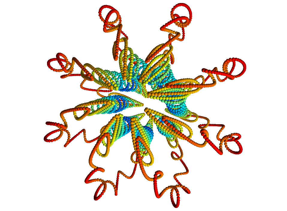
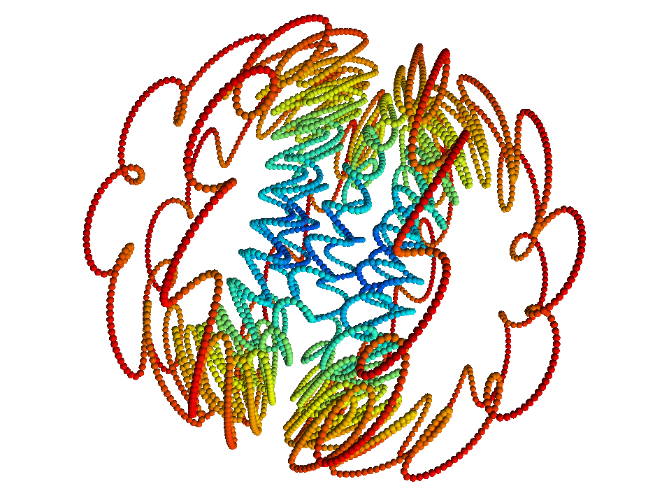
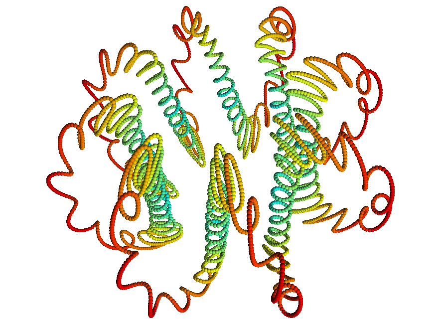
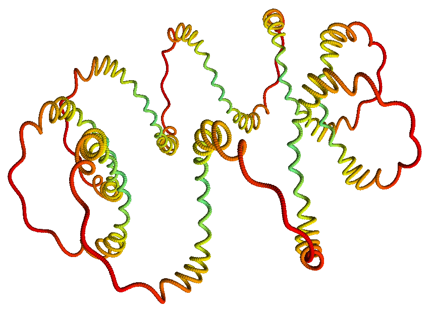
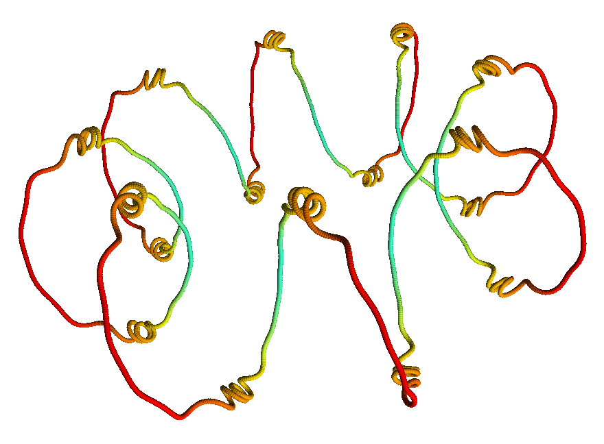
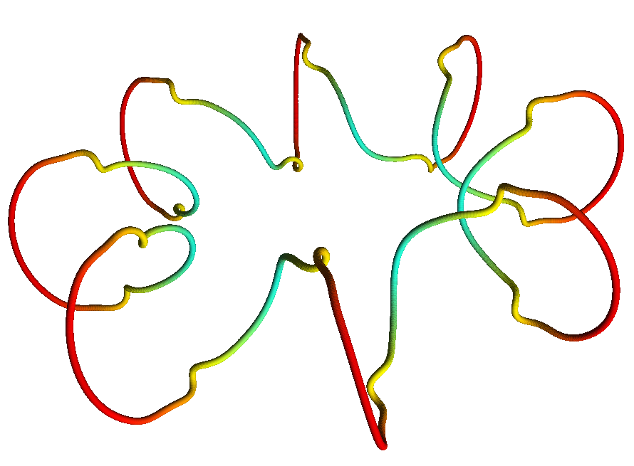
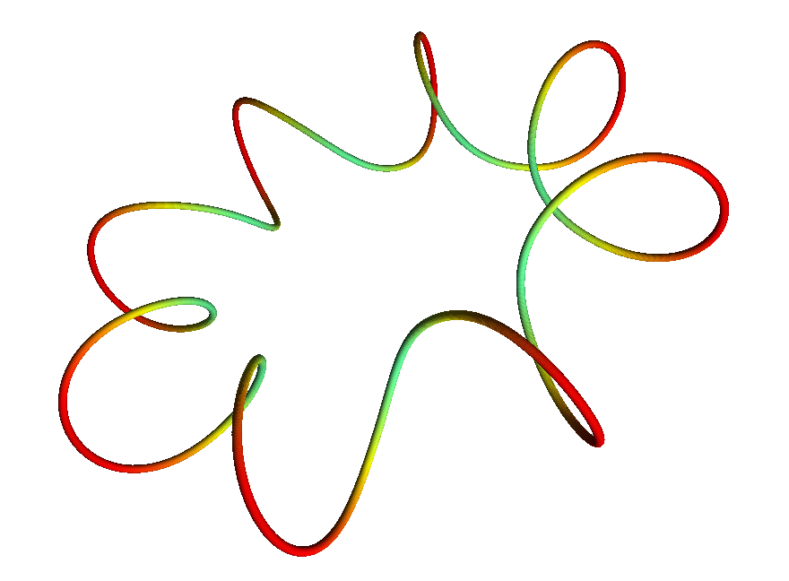
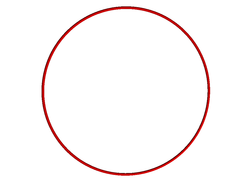
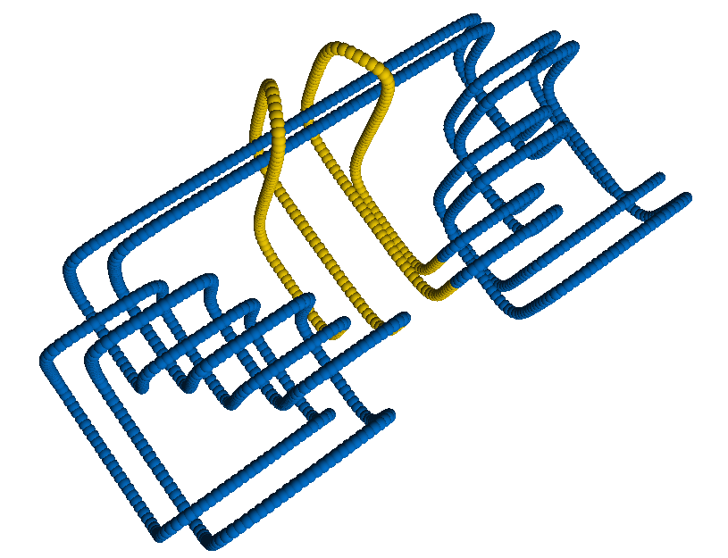
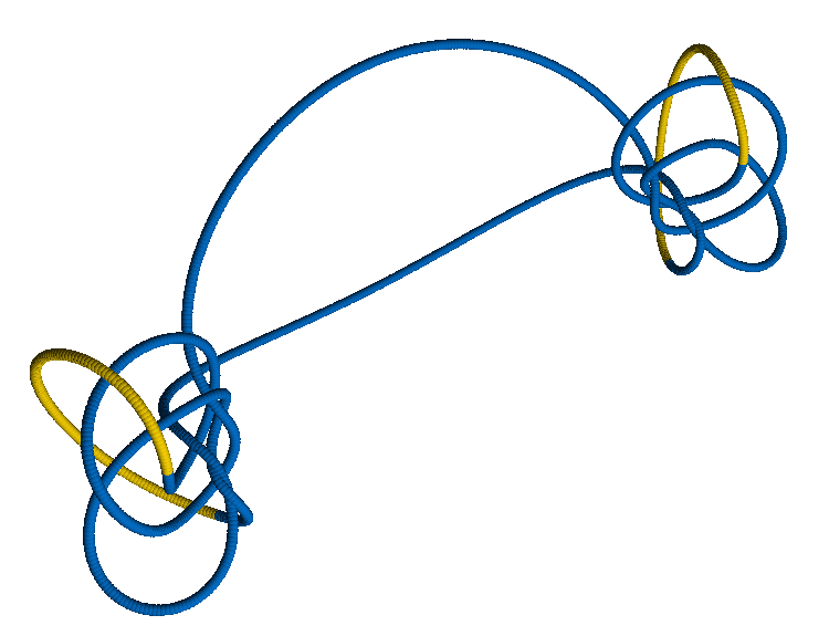
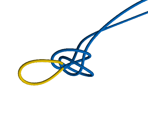
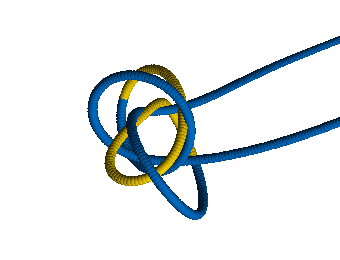
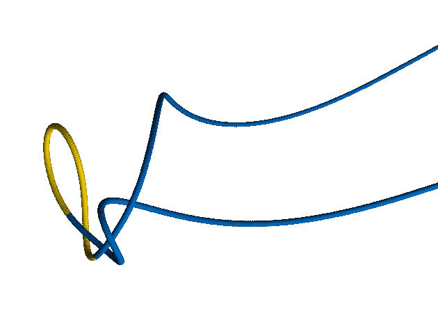
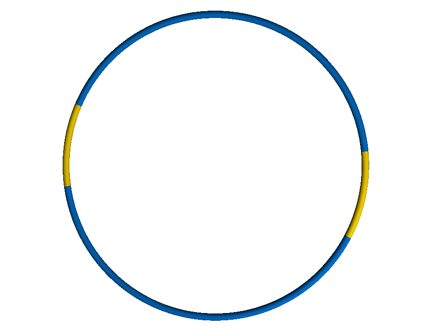
Figure 2 also explores the “dynamic” Smale conjecture, but for a pathologically difficult embedding of the unknot. It illustrates the dynamics of (56) for an example lying within a well-known infinite family of “hard” unknots constructed by taking the connected sum of two knots (in this instance, both trefoils), doubling the resulting knot by forming an index-two cable of the connected sum and finally performing surgery on the cable knot in a neighborhood of the summing sphere in order to produce an unknot. The original knot deforms to the standard unknot by first isotoping the yellow strands around the large knotted bodies on either symmetric side of the structure. Pulling along the “tracks” of the doubled trefoil structures then eliminates the knotted bodies, which results in a planar embedding of the unknot. The dynamics of (56) provide an approximate version of this process. We simulate (56) using the -Distortion for this example with an initial condition scaled to have initial equipartition of energy as before. Panels (b,c) of figure 2 show the initial phase wherein the yellow strands isotope around the knotted bodies. This process has finished by , and afterward the two yellow strands begin to pull through the trefoil structures. Panels (c,d) show the onset and midpoint of this process for the left side of the structure; the dynamics for the right of the structure are simply the mirror image across the initial plane of symmetry. By shown in panel (e), the embedding differs from the standard embedding of the unknot only by trivial twisting. The remaining dynamics simply perform local rotations of arcs of the embedding to perform the final simplification of the structure into the standard unknot.
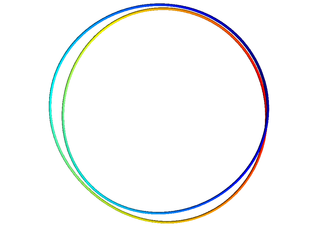
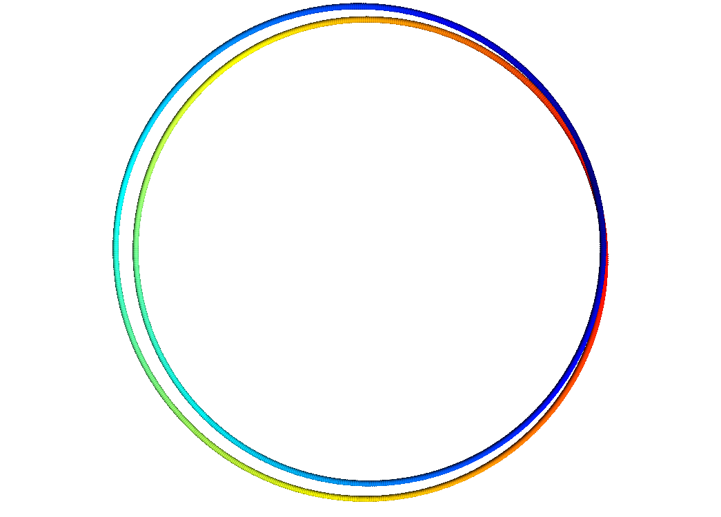
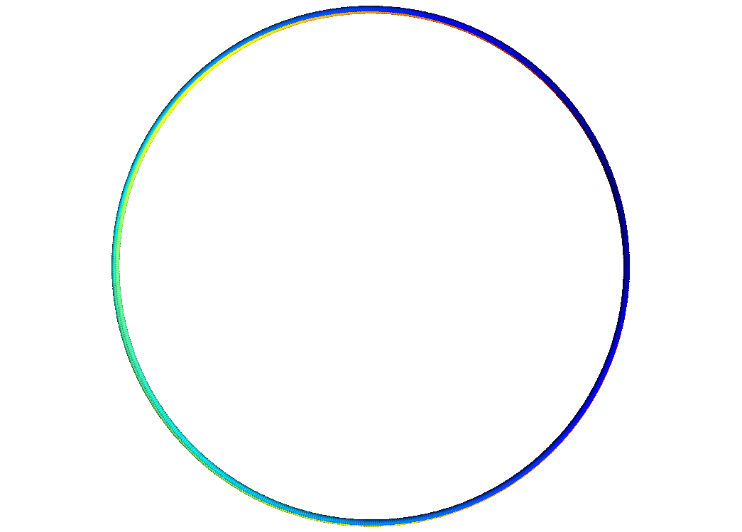
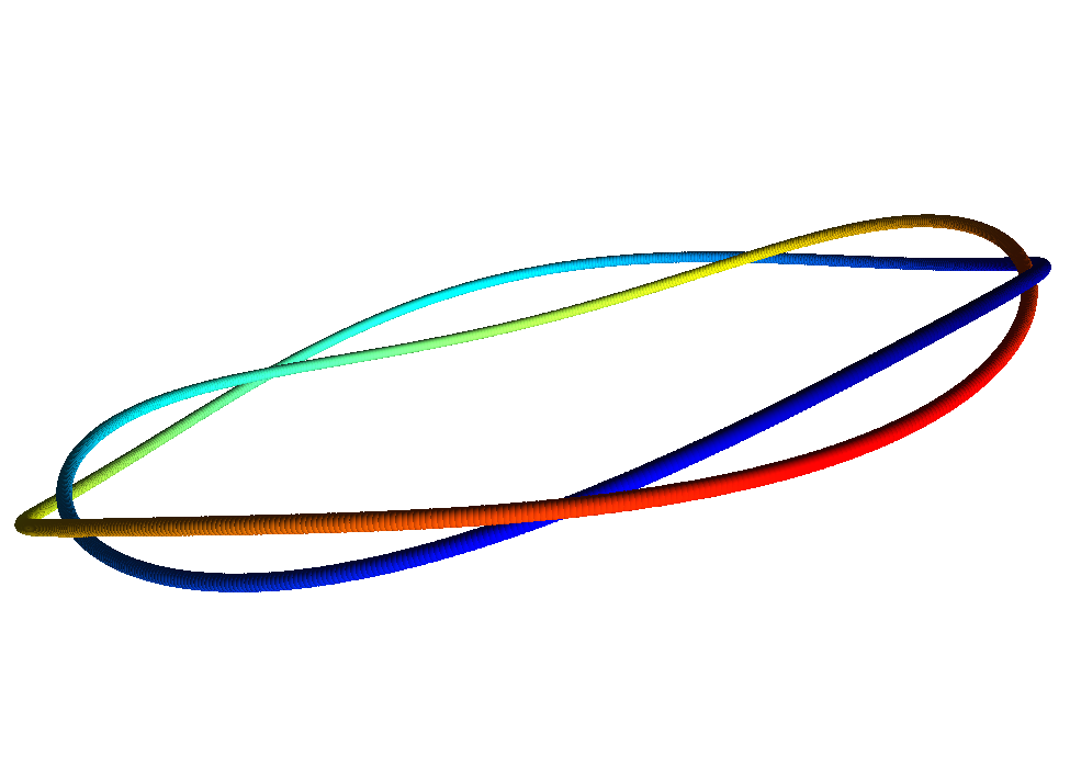
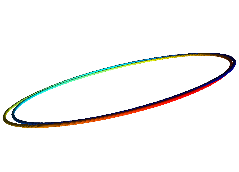
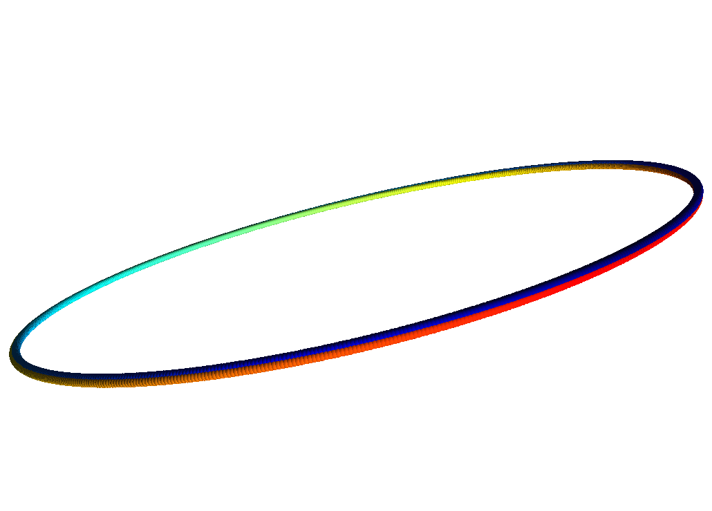
We conclude our experiments with a numerical simulation illustrating how, in the absence of the repulsive energy the dynamics of (56) can flow unknots into the double-covered circle. We use the unknotted initial condition
from section 4.4.2 with and and simulate a pure bending energy flow. Figure 3 illustrates that the dynamics do, in fact, obey our approximation
to leading-order. The binormal component of (i.e. the -axis) vanishes exponentially quickly, as shown in panel (b,d), in comparison to the dynamics occuring in the plane. These planar dynamics then simply equilibrate the inner and outer “circles” until both coincide, yielding the double-covered circle. In particular, at each stage there exists a projection of onto the plane with a single crossing, as in figure 3 (b), and while their preimages are exponentially close they are, in fact, distinct. In other words remains unknotted for all time yet is emphatically not the global minimizer of the bending energy within the ambient isotopy class of the unknot. So while the “dynamic” Smale conjecture plausibly holds in the presence of a repulsive energy this example demonstrates that it is emphatically false in its absence of such a repulsive force. This example is perhaps not surprising, but it nevertheless cautions against a naive intuition about how a realization of the “dynamic” Smale conjecture might unfold. Specifically, the fact that an energy yields as its global minimizer in no way implies that a corresponding notion of “convexity” with respect to the unknot type must hold.
6 Conclusion
Our present focus lies on those particular instances of the general family (1) that contain two main physical effects, namely curvature-driven diffusion and nonlocal repulsion. Combining these effects yields a strong energetic model from a combinatorial complexity point-of-view, as lemma 3.3 shows. A weak repulsion (as weak as the Distortion) combines with a fractional diffusion ( for ) to give a rather strong (say finite-to-one) invariant. In the physically relevant case () these effects lead to a set of dynamical models with well-behaved dynamics, in the sense that they exhibit desirable global existence and regularity properties for a large class of nonlocal kernels (c.f. theorem 4.13). These dynamics themselves, in particular their doubly-nonlocal nature, appear novel and also admit reliable numerical approximation wherein self-intersections are easy to avoid. A further analysis highlights a few aspects of the dynamics themselves. In the presence of repulsion, techniques for nonlocal dynamical systems show that standard circles are orbitally stable at a local level, while at a global level numerical experiments reveal that the basin of attraction for circles contains rather complex initial embeddings. We use a similar combination of techniques to illustrate a simple but important observation, that in the absence of repulsion there exist unknotted initial configurations that remain unknotted for all time under a bending energy flow, yet the dynamics do not asymptotically converge to the globally minimal, unknotted circle. Finally, the overall methodology, and in particular the equilibrium analysis, extends readily to related settings such as systems of interacting curves (e.g. knots and links) or to nonlocal interactions involving both attraction and repulsion. Studying variants along these lines provide fertile ground for future work, as does a more in-depth study of the weighted crossing number (13) from a purely knot-theoretic point-of-view.
References
- [1] C.-M. Chen, C.-C. Chen, Computer simulations of membrane protien foldling: Structure and dynamics, Biophysical Journal 84 (2003) 1902–1908.
- [2] A. Calini, T. Ivey, Finite-gap solutions to the vortex filament equation: Genus one solutions and symetric solutions, J. Nonlinear Sci. 15 (2005) 321–361.
-
[3]
C.-C. Lin, H. R. Schwetlick,
On a flow to untangle
elastic knots, Calc. Var. Partial Differential Equations 39 (3-4) (2010)
621–647.
doi:10.1007/s00526-010-0328-0.
URL http://dx.doi.org/10.1007/s00526-010-0328-0 -
[4]
O. Gonzalez, J. H. Maddocks,
Global curvature, thickness,
and the ideal shapes of knots, Proc. Natl. Acad. Sci. USA 96 (9) (1999)
4769–4773.
doi:10.1073/pnas.96.9.4769.
URL http://dx.doi.org/10.1073/pnas.96.9.4769 -
[5]
P. Strzelecki, H. von der Mosel,
Menger curvature as a
knot energy, Phys. Rep. 530 (3) (2013) 257–290.
doi:10.1016/j.physrep.2013.05.003.
URL http://dx.doi.org/10.1016/j.physrep.2013.05.003 - [6] S. Blatt, The gradient flow of o’hara’s knot energies, arXiv:1601.02840.
- [7] S. Blatt, The gradient flow of the Möbius energy: -regularity and consequences, 1601.07023.
-
[8]
K. A. Hoffman, T. I. Seidman,
A variational rod model
with a singular nonlocal potential, Arch. Ration. Mech. Anal. 200 (1) (2011)
255–284.
doi:10.1007/s00205-010-0368-9.
URL http://dx.doi.org/10.1007/s00205-010-0368-9 - [9] S. Blatt, P. Reiter, Modeling repulsive forces on fibres via knot energies.
-
[10]
J. W. Milnor, On the total curvature
of knots, Ann. of Math. (2) 52 (1950) 248–257.
doi:10.2307/1969467.
URL http://dx.doi.org/10.2307/1969467 -
[11]
M. H. Freedman, Z.-X. He, Z. Wang,
Möbius energy of knots and
unknots, Ann. of Math. (2) 139 (1) (1994) 1–50.
doi:10.2307/2946626.
URL http://dx.doi.org/10.2307/2946626 -
[12]
J. Cantarella, R. B. Kusner, J. M. Sullivan,
On the minimum ropelength
of knots and links, Invent. Math. 150 (2) (2002) 257–286.
doi:10.1007/s00222-002-0234-y.
URL http://dx.doi.org/10.1007/s00222-002-0234-y -
[13]
G. Buck, J. Simon,
Thickness and crossing
number of knots, Topology Appl. 91 (3) (1999) 245–257.
doi:10.1016/S0166-8641(97)00211-3.
URL http://dx.doi.org/10.1016/S0166-8641(97)00211-3 -
[14]
S. Blatt, P. Reiter, Regularity
theory for tangent-point energies: the non-degenerate sub-critical case,
Adv. Calc. Var. 8 (2) (2015) 93–116.
doi:10.1515/acv-2013-0020.
URL http://dx.doi.org/10.1515/acv-2013-0020 -
[15]
S. Blatt, P. Reiter,
Stationary points of
O’Hara’s knot energies, Manuscripta Math. 140 (1-2) (2013) 29–50.
doi:10.1007/s00229-011-0528-8.
URL http://dx.doi.org/10.1007/s00229-011-0528-8 -
[16]
S. Blatt, P. Reiter, Towards a
regularity theory for integral Menger curvature, Ann. Acad. Sci. Fenn.
Math. 40 (1) (2015) 149–181.
doi:10.5186/aasfm.2015.4006.
URL http://dx.doi.org/10.5186/aasfm.2015.4006 -
[17]
S. Blatt, P. Reiter, A. Schikorra,
Harmonic analysis meets critical
knots. Critical points of the Möbius energy are smooth, Trans. Amer.
Math. Soc. 368 (9) (2016) 6391–6438.
doi:10.1090/tran/6603.
URL http://dx.doi.org/10.1090/tran/6603 - [18] J. Cantarella, J. H. Fu, R. B. Kusner, J. M. Sullivan, Ropelength criticality, Geometry & Topology 18 (4) (2014) 2595–2665.
-
[19]
E. Denne, J. M. Sullivan,
The distortion of a
knotted curve, Proc. Amer. Math. Soc. 137 (3) (2009) 1139–1148.
doi:10.1090/S0002-9939-08-09705-0.
URL http://dx.doi.org/10.1090/S0002-9939-08-09705-0 -
[20]
R. A. Litherland, J. Simon, O. Durumeric, E. Rawdon,
Thickness of knots,
Topology Appl. 91 (3) (1999) 233–244.
doi:10.1016/S0166-8641(97)00210-1.
URL http://dx.doi.org/10.1016/S0166-8641(97)00210-1 -
[21]
E. Denne, Y. Diao, J. M. Sullivan,
Quadrisecants give new lower
bounds for the ropelength of a knot, Geom. Topol. 10 (2006) 1–26.
doi:10.2140/gt.2006.10.1.
URL http://dx.doi.org/10.2140/gt.2006.10.1 -
[22]
J. O’Hara, Energy of a
knot, Topology 30 (2) (1991) 241–247.
doi:10.1016/0040-9383(91)90010-2.
URL http://dx.doi.org/10.1016/0040-9383(91)90010-2 - [23] J. O’Hara, Energy functionals of knots, in: Topology Hawaii (Honolulu, HI, 1990), World Sci. Publ., River Edge, NJ, 1992, pp. 201–214.
-
[24]
J. O’Hara, Family of
energy functionals of knots, Topology Appl. 48 (2) (1992) 147–161.
doi:10.1016/0166-8641(92)90023-S.
URL http://dx.doi.org/10.1016/0166-8641(92)90023-S -
[25]
J. O’Hara, Energy
functionals of knots. II, Topology Appl. 56 (1) (1994) 45–61.
doi:10.1016/0166-8641(94)90108-2.
URL http://dx.doi.org/10.1016/0166-8641(94)90108-2 -
[26]
A. Abrams, J. Cantarella, J. H. G. Fu, M. Ghomi, R. Howard,
Circles minimize most
knot energies, Topology 42 (2) (2003) 381–394.
doi:10.1016/S0040-9383(02)00016-2.
URL http://dx.doi.org/10.1016/S0040-9383(02)00016-2 -
[27]
S. Blatt, The gradient flow
of the Möbius energy near local minimizers, Calc. Var. Partial
Differential Equations 43 (3-4) (2012) 403–439.
doi:10.1007/s00526-011-0416-9.
URL http://dx.doi.org/10.1007/s00526-011-0416-9 - [28] H. Gerlach, P. Reiter, H. von der Mosel, The elastic trefoil is the twice covered circle, Arch. Rat. Mech. Anal. 225 (1) (2017) 89–139.
- [29] P. Strzelecki, H. von der Mosel, Tangent-point self-avoidance energies for curves, J. Knot Theory Ramifications 21 (5).
- [30] E. M. Stein, R. Shakarchi, Real analysis: measure theory, integration, and Hilbert spaces, Princeton University Press, 2009.
- [31] J. H. von Brecht, S. G. McCalla, Nonlinear stability through algebraically decaying point spectrum: Applications to nonlocal interaction equations, SIAM Journal on Mathematical Analysis 46 (6) (2014) 3727–3760.
- [32] M. Gromov, Structures métriques pour les variétés riemanniennes, Vol. 1 of Textes Mathématiques [Mathematical Texts], CEDIC, Paris, 1981, edited by J. Lafontaine and P. Pansu.
- [33] P. Reiter, All curves in a -neighborhood of a given embedded curve are isotopic, Report 4, Institut fr Mathematik, RWTH Aachen 2005.
-
[34]
J. Langer, D. A. Singer,
Curve straightening and
a minimax argument for closed elastic curves, Topology 24 (1) (1985) 75–88.
doi:10.1016/0040-9383(85)90046-1.
URL http://dx.doi.org/10.1016/0040-9383(85)90046-1 -
[35]
M. H. Freedman, Z.-X. He,
Divergence-free fields: energy and
asymptotic crossing number, Ann. of Math. (2) 134 (1) (1991) 189–229.
doi:10.2307/2944336.
URL http://dx.doi.org/10.2307/2944336 - [36] V. I. Arnold, The asymptotic Hopf invariant and its applications, Selecta Math. Soviet. 5 (4) (1986) 327–345, selected translations.
- [37] H. Federer, Geometric measure theory, Springer, 2014.
-
[38]
M. Gromov, Homotopical
effects of dilatation, J. Differential Geom. 13 (3) (1978) 303–310.
URL http://projecteuclid.org/euclid.jdg/1214434601 - [39] D. Henry, Geometric theory of semilinear parabolic equations, Vol. 840, Springer-Verlag Berlin, 1981.
- [40] R. C. McOwen, Partial differential equations: Methods and applications (2nd ed.), Pearson Education, 2003.
- [41] J. H. von Brecht, Localization and vector spherical harmonics, Journal of Differential Equations 260 (2) (2016) 1622–1655.
-
[42]
D. von Brecht, James H.and Uminsky,
Anisotropic assembly and
pattern formation, Nonlinearity 30 (1) (2017) 225–273.
doi:10.1088/1361-6544/30/1/225.
URL http://dx.doi.org/10.1088/1361-6544/30/1/225 - [43] T. Kapitula, K. Promislow, Spectral and dynamical stability of nonlinear waves, Springer, 2013.
-
[44]
J. Langer, D. A. Singer,
The total squared
curvature of closed curves, J. Differential Geom. 20 (1) (1984) 1–22.
URL http://projecteuclid.org/euclid.jdg/1214438990
7 Appendix
Lemma 7.1.
(Lemma 3.1) Assume that satisfies the homogeneity property
for some exponent and some function . Assume that the lower bound holds on as well. If has unit speed then
for finite constants. Moreover, if then
and so is bi-Lipschitz if is finite.
Proof.
Let denote a distortion-realizing pair so that
where denotes the maximal distance between a distortion realizing pair. For any two such points and define
and use the -Lipschitz property of along with the inequality to estimate
for any pair of arbitrary points and an arbitrary parameter. Define as
the latter inequality holding due to the previous estimate. In particular, if the pair lies in the set
then and so
holds as well. As the lower bound
holds for all sufficiently large and sufficiently small. For example, for and , it therefore follows that on and so the lower bound
follows. Now make the change of variables and and use the -periodicity of to find
where the last inequality follows by shifting to polar coordinates. Performing the final integration then shows
The final claim also follows from this inequality by noting that (c.f.(6)).
for a universal constant. ∎
Lemma 7.2.
(Lemma 3.3) Assume that and that has finite distortion. Assume further that has constant speed. Then
and if then the constant
is finite.
Proof.
That has constant speed yields and so the relations
furnish the distortion and pointwise curvature. Note first that the equality
holds by the definition of and the trilinearity of the triple product. Set and note that the inequality
also holds by definition of the triple product. Moreover, as has constant speed. Finally by definition of the distortion. Thus
Now apply Cauchy-Schwarz to find
But and Parseval imply
where the last equality follows from a simple change of variables. A similar argument shows that
as well. Collecting constants and extending the region of integration then yields the claim. ∎
Lemma 7.3.
(Lemma 4.1) If and then the linear operator
| (58) |
defines an function. As a Fourier multiplier it acts as a (negative) fractional Laplacian
and in particular the operator-norm estimate
holds.
Proof.
Consider first the linear operator defined, for by the expression
The last equality follows from periodicity of and a change of variables. Now expand in a Fourier series to conclude
with equality holding in the sense. For a change of variables then gives
where the error holds uniformly in and in . As and the desired estimate
then follows. ∎
Lemma 7.4.
(Lemma 4.2) Assume that is homogeneous and either -degenerate or -degenerate. Assume that is a unit speed, bi-Lipschitz embedding. Then for the function
has mean zero. Moreover, obeys a uniform bound
for an -independent constant.
Proof.
That has mean zero follows from the antisymetry of the integrand. As defines a unit speed, bi-Lipschitz embedding, there exists a so that
for the distortion of the curve. As has unit speed, also satisfies
for the curvature maximal function (c.f. (7)). Define which obeys the bounds . Then by the -homogeneity hypothesis,
The estimate then follows from this expression by appealing to one of the degeneracy assumptions.
First consider the -Degenerate case. Then by assumption, and so for any there exists so that
by the mean value theorem. Combining these inequalities then gives
Thus and the latter lies in by the boundedness of the curvature maximal function. Combining this with the previous lemma for yields the claim in this case.
Now suppose is degenerate with and so there exists with
due to the degeneracy assumption. Thus
The last inequality follows from the fact that by assumption. Thus is bounded in uniformly with respect to as claimed. ∎
Lemma 7.5.
(Lemma 4.3) Assume that is homogeneous and either -degenerate or -degenerate. Let denote unit speed, bi-Lipschitz embeddings. Then for the uniform Lipschitz estimates
hold, where denotes an -independent constant.
Proof.
Take and so that
as in the proof of the previous lemma. Define and similarly.
Assume first that -Degeneracy holds. By defining and a trivial calculation shows that
The fact that follows immediately from lemma 4.1. As for arguing as in the previous lemma shows
and so obeys
as desired. Finally, the mean value theorem once again furnishes a so that
Noting that
| (59) |
then yields the estimate
for the third term. From the definition of and it follows that
| (60) |
That and have unit speed then gives
which yields the desired estimate
for the third term. Combining these estimates yields the claim
in the -Degenerate case.
Assume now that -Degeneracy holds. Then
as before. That obeys the claimed bound then follows by using the argument of the previous lemma. Now decompose into two pieces,
For there exists a so that
Furthermore, there exists a so that
As a consequence, this bound furnishes the inequality
Recalling (7) and the bounds (59) and (60)
and arguing as before then completes the estimate
for this term. The estimate for then follows by the same argument with in place of , so the claimed bound holds in the -Degenerate case as well. ∎
Lemma 7.6.
(Lemma 4.4) Suppose that and that
for a positive constant. If is non-constant then
is non-singular. The operator norm estimate
also holds, and so exists and obeys
whenever is sufficiently small.
Proof.
Select with unit length so that the quadratic form realizes the minimal eigenvalue. A simple computation reveals
by Cauchy-Schwarz. As varies continuously on equality holds if and only if and are everywhere collinear. But is non-constant, so equality cannot occur. Thus and so exists.
Now take with unit length but otherwise arbitrary. Then
and so the claimed operator norm estimate
follows. The simple eigenvalue inequality yields invertibility of for sufficiently small, while the trivial identity yields the final estimate. ∎
Proposition 7.7.
(Proposition 4.6) Suppose for arbitrary. Then for any initial datum the linear initial value problem
| (61) |
has a unique mild solution . For any the solution obeys the estimate
for a universal constant.
Proof.
For each define the coefficients of the solution as
| (62) |
so that for fixed the fact that gives
The series therefore lies in , and so for both functions
define functions with estimates
The claimed bound for therefore follows from the triangle inequality. The claim that follows in a similar way, i.e. by first shifting the temporal origin from to and then applying the argument estimating to the difference on the interval . Finally, the claim that
for is standard. For simply define
and apply the Fubini-Tonelli theorem. Thus with coefficients defined by (62) yields the unique mild solution. ∎
Lemma 7.8.
(Lemma 4.9) Assume that is homogeneous and degenerate. Assume that is a unit speed, bi-Lipschitz embedding. Then the nonlocal integral
lies in and obeys the estimate
for a continuous function of its arguments.
Proof.
Assume first that the claim holds for all that are bi-Lipschitz, unit speed and smooth. Take a sequence of smooth functions with unit speed converging to in the norm. In particular, the convergence
holds as well, as does the limit in by lemma 4.3. The bound
guarantees that weakly for some after passing to a subsequence if necessary. Then for any smooth, -periodic function the equality
holds for all which upon passing to the limit using weak convergence shows that
for any smooth function. Thus provides a weak derivative for . But then
and so the claim holds in the general case.
It therefore suffices to prove the claim for smooth functions. Given define according to
and as well. A simple argument using Taylor’s theorem shows that
In the -degenerate case,
The proof of lemma 4.1 shows that
but and so the first term lies in as desired. For the second term, first define and then let
denote its integrand. Note that implies
| (63) |
for a universal constant. The fact that
combines with the homogeneity and -degeneracy assumptions to show
and so we may apply the bound (7) for and the continuous embedding to the first term and the argument of lemma 4.2 (with in place of ) to the second term to conclude
As the maximal function is uniformly bounded for smooth functions and the latter expression is integrable, the differentiation formula
is therefore valid. The claimed bound
then follows by the boundedness of the maximal function. This completes the proof in the -degenerate case.
The -degenerate case follows in a similar fashion. In this instance the expression
is valid. Define and as before. Note that having a root of order at shows that has a root of order at as well. Arguing as in lemma 4.2 yields the estimate
Now recall that and that is a non-negative integer by hypothesis. Thus and so the claimed bound then follows by arguing as in the -degenerate case. ∎
Corollary 7.9.
Proof.
Let
denote the existence times of mild solutions and its positive supremum. If take a monotone sequence of times realizing this supremum, in the sense that
Let denote the corresponding mild solution. Note first that on by uniqueness of mild solutions, and so on we may consider as a single, well-defined and -valued mapping. Assume that we have a-priori and distortion bounds for the solution, by which we mean that
are finite. By standard compactness results we may extract a subsequence of the and infer that there exists so that
hold for an arbitrary exponent. Thus has zero mean and unit speed. We therefore infer that
By theorem 4.10 we may then infer that
is finite as well. Appealing to standard compactness results once again then shows that, by passing to a further subsequence if necessary, we may assume
| (64) |
without loss of generality. The induced embeddings therefore converge in and so in particular
is finite by the distortion a-priori bound. Thus induces a bi-Lipschitz embedding, and so we may infer that
| (65) |
Now apply theorem 4.8 with as initial data to find some and a defining a mild solution. Define piecewise by
and note that (64) shows that is, in fact, continuous. By using (65) it is then easy to show that defines a mild solution with as initial data. Thus a contradiction. ∎