Variance-based sensitivity analysis for time-dependent processes

Abstract

The global sensitivity analysis of time-dependent processes requires history-aware approaches. We develop for that purpose a variance-based method that leverages the correlation structure of the problems under study and employs surrogate models to accelerate the computations. The errors resulting from fixing unimportant uncertain parameters to their nominal values are analyzed through a priori estimates. We illustrate our approach on a harmonic oscillator example and on a nonlinear dynamic cholera model.

1 Introduction

The ability to make reliable predictions from time-dependent mathematical models of the form

$$Y=f(t,{\mathchoice{\mbox{\boldmath$\displaystyle{\xi}$}}{\mbox{\boldmath$\textstyle{\xi}$}}{\mbox{\boldmath$\scriptstyle{\xi}$}}{\mbox{\boldmath$\scriptscriptstyle{\xi}$}}}),\quad t\in[0,T],$$ (1)

where ${\mathchoice{\mbox{\boldmath$\displaystyle{\xi}$}}{\mbox{\boldmath$\textstyle{\xi}$}}{\mbox{\boldmath$\scriptstyle{\xi}$}}{\mbox{\boldmath$\scriptscriptstyle{\xi}$}}}\in\mathbb{R}^{N_{\text{p}}}$ is a vector of uncertain model parameters, relies crucially on understanding and quantifying the impact of $\textstyle{\xi}$ on $f$. One approach, due to Sobol’, consists in apportioning to each element (or group of elements) of $\textstyle{\xi}$ its contribution to the variance of $f$ [1, 2, 3, 4]. Such a global sensitivity analysis (GSA) enables focusing computational resources on quantifying the uncertainties in the elements of $\textstyle{\xi}$ that are most influential on the variability of $f$. The present work is about extending Sobol’s approach to problems with time-dependent outputs.

Most of the literature on global sensitivity analysis considers scalar outputs as opposed to the functional framework corresponding to (1). This amounts, for instance, to analyzing the sensitivity of $f(t_{0},{\mathchoice{\mbox{\boldmath$\displaystyle{\xi}$}}{\mbox{\boldmath$\textstyle{\xi}$}}{\mbox{\boldmath$\scriptstyle{\xi}$}}{\mbox{\boldmath$\scriptscriptstyle{\xi}$}}})$ for a fixed $t_{0}$ or to the study of integrated quantities such as $y({\mathchoice{\mbox{\boldmath$\displaystyle{\xi}$}}{\mbox{\boldmath$\textstyle{\xi}$}}{\mbox{\boldmath$\scriptstyle{\xi}$}}{\mbox{\boldmath$\scriptscriptstyle{\xi}$}}})=\int_{0}^{T}f(t,{\mathchoice{\mbox{\boldmath$\displaystyle{\xi}$}}{\mbox{\boldmath$\textstyle{\xi}$}}{\mbox{\boldmath$\scriptstyle{\xi}$}}{\mbox{\boldmath$\scriptscriptstyle{\xi}$}}})\,dt$. While it is possible to apply Sobol’s approach pointwise in time [5, 6], for instance at the nodes of a grid,

$$0=t_{0}<t_{1}<\cdots<t_{n-1}<t_{n}=T,$$ (2)

this approach presents two shortcomings. First, treating the $f(t_{k},{\mathchoice{\mbox{\boldmath$\displaystyle{\xi}$}}{\mbox{\boldmath$\textstyle{\xi}$}}{\mbox{\boldmath$\scriptstyle{\xi}$}}{\mbox{\boldmath$\scriptscriptstyle{\xi}$}}})$’s, $k=1,\dots,n$, independently of one another ignores the temporal correlation structure of the process. Second, the variance of the process itself varies in time therefore skewing relative importance measurements across time. More precisely, a “yardstick” is needed at each time to determine the influential parameters at that time; for the standard Sobol’s indices, this yardstick is the variance of $f$ at the corresponding time. When the yardstick changes with time, confusion ensues: how to compare carrying a small portion of a large variance with a large portion of a small one? These delicate scaling issues are also present in derivative-based sensitivity analysis.

As an illustrative example, consider an underdamped mechanical oscillator whose motion is governed by the initial value problem

$$y^{\prime\prime}+2\alpha y^{\prime}+(\alpha^{2}+\beta^{2})y=0,$$ (3)

$$y(0)=\ell,\quad y^{\prime}(0)=0.$$

The solution is

$$y(t;\alpha,\beta,\ell)=\ell e^{-\alpha t}(\cos\beta t+\frac{\alpha}{\beta}\sin\beta t),$$ (4)

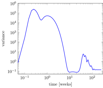
and the corresponding process is given by $f(t,{\mathchoice{\mbox{\boldmath$\displaystyle{\xi}$}}{\mbox{\boldmath$\textstyle{\xi}$}}{\mbox{\boldmath$\scriptstyle{\xi}$}}{\mbox{\boldmath$\scriptscriptstyle{\xi}$}}})=y(t;{\mathchoice{\mbox{\boldmath$\displaystyle{\xi}$}}{\mbox{\boldmath$\textstyle{\xi}$}}{\mbox{\boldmath$\scriptstyle{\xi}$}}{\mbox{\boldmath$\scriptscriptstyle{\xi}$}}})$, where $\textstyle{\xi}$ is a random vector that parameterizes the uncertainty in the parameters $(\alpha,\beta,\ell)$. Figure 1 (left) shows the time evolution of the mean trajectory (solid line) and the two standard deviation bounds (dashed lines). The values of the traditional pointwise total Sobol’ indices, which we recall in Section 2, are reported in Figure 1 (right).

Figure 1: Behavior of the mechanical oscillator problem (3) with uncertain parameters $\alpha\sim\mathcal{U}(3/8,5/8)$, $\beta\sim\mathcal{U}(10/4,15/4)$ and $\ell\sim\mathcal{U}(-5/4,-3/4)$. Left: mean trajectory $\bar{y}(t)$ and the two standard deviation bounds, obtained via Monte Carlo sampling in the uncertain parameter space. Right: standard Sobol’ indices over time.

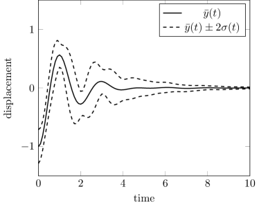
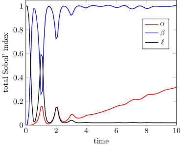
These results are difficult to interpret as the balance of sensitivities changes multiple times. Moreover, this standard approach is entirely unaware of the history of the process and, specifically here, of the asymptotically diminishing variance. For instance, the reported increasing influence of $\alpha$ is largely an artifact of the method. We revisit this example throughout the article and, in Section 5, investigate similar issues on a more involved dynamical system modeling the spread of cholera.

Porting variance based GSA methods from the scalar case to the vectorial case or, more generally, to the functional case corresponding to (1) presents three challenges:

1. the yardstick issue,

2. the need for a functional framework allowing analysis and method development,

3. the need for a computational framework allowing the implementation of efficient algorithms on realistic problems and applications.

Our work is motivated by [7] which resolves challenge I in a general setting. We offer here key contributions to the resolutions of challenges II and III.

• We establish in Section 4 the equivalence of the indices from [7] to those previously proposed in [8]; see Theorem 4.1.

• We analyze, in the functional case, the effect of fixing inessential variables as determined by computing generalized Sobol’ indices. This is done theoretically in Section 3 and is thoroughly investigated in the numerical results in Section 5.

• We leverage our representation of the generalized indices to enable the analysis and efficient implementation of two distinct approaches for the computation of these indices, namely surrogate models (see Section 4.1) and spectral representations (see Section 4.2).

• We present comprehensive numerical results that provide insight into sensitivity analysis of time-dependent processes; additionally, our numerical results examine various aspects of our methods and show their effectiveness.

We conclude this Introduction with a brief overview of surrogate models and spectral representations in the context of functional GSA.

Surrogate models such as polynomial chaos (PC) expansions [9, 10, 11], multivariate adaptive regression splines (MARS) [12], and Gaussian processes have become increasingly popular tools in uncertainty quantification literature; the references [13, 14, 15, 16, 17, 18, 19] provide a non-exhaustive sample of the literature on their use for variance-based sensitivity analysis. These approaches replace repeated solutions of computationally expensive models by inexpensive evaluations of a surrogate model. They can provide orders of magnitude speedups. While our approach is agnostic the choice of surrogates, we use PC surrogates in our implementation. In practice, the choice of surrogate model should be based on the demands of the problem at hand. In the present context, a surrogate model $\tilde{f}(t_{k},{\mathchoice{\mbox{\boldmath$\displaystyle{\xi}$}}{\mbox{\boldmath$\textstyle{\xi}$}}{\mbox{\boldmath$\scriptstyle{\xi}$}}{\mbox{\boldmath$\scriptscriptstyle{\xi}$}}})\approx f(t_{k},{\mathchoice{\mbox{\boldmath$\displaystyle{\xi}$}}{\mbox{\boldmath$\textstyle{\xi}$}}{\mbox{\boldmath$\scriptstyle{\xi}$}}{\mbox{\boldmath$\scriptscriptstyle{\xi}$}}})$ can be constructed for every $t_{k}$ in the grid (2) and generalized indices can subsequently be approximated at negligible computational cost (see again Section 4.1). However, the full approximating power of many state-of-the-arts surrogates can only be harvested at the price of optimizing them at each specific time $t_{k}$. This may be prohibitively expensive and intractable especially when the number of time steps $n$ is large.

This observation motivates the consideration of spectral representations and, specifically here, the Karhunen–Loève (KL) expansion

$$f(t,{\mathchoice{\mbox{\boldmath$\displaystyle{\xi}$}}{\mbox{\boldmath$\textstyle{\xi}$}}{\mbox{\boldmath$\scriptstyle{\xi}$}}{\mbox{\boldmath$\scriptscriptstyle{\xi}$}}})\approx f_{0}(t)+\sum_{j=1}^{N_{\text{kl}}}f_{i}({\mathchoice{\mbox{\boldmath$\displaystyle{\xi}$}}{\mbox{\boldmath$\textstyle{\xi}$}}{\mbox{\boldmath$\scriptstyle{\xi}$}}{\mbox{\boldmath$\scriptscriptstyle{\xi}$}}})e_{i}(t),$$

of the process $f$, where $f_{0}$ is the mean of the process, the $f_{i}({\mathchoice{\mbox{\boldmath$\displaystyle{\xi}$}}{\mbox{\boldmath$\textstyle{\xi}$}}{\mbox{\boldmath$\scriptstyle{\xi}$}}{\mbox{\boldmath$\scriptscriptstyle{\xi}$}}})$’s are expansion coefficients (see Section 4.2) with variance $\mathbb{V}\left\{{f_{i}}\right\}=\lambda_{i}$ and where $\lambda_{i}$ is an eigenvalue of the covariance operator of $f$ with corresponding eigenvector $e_{i}$. The modes $\{f_{i}\}_{i=1}^{N_{\text{kl}}}$ encode the uncertainty in $f$ and the dynamics of the process is quantified by the superposition of the dominant eigenvectors $\{e_{i}\}_{i=1}^{N_{\text{kl}}}$. For processes with fast decaying eigenvalues $\lambda_{i}$—which is often observed in applications—a small truncation level ${N_{\text{kl}}}$ can be used, i.e., the process can be represented by a small number of modes.

The principle and feasibility of functional GSA based on spectral representations are explored in [20]. These ideas are picked up in [8] (see also [21]) where aggregate Sobol’ indices are proposed for vectorial and functional outputs, based on the KL expansion of $f$. The unifying theoretical framework of Section 4.2 is here completed by a thorough discussion of the computational issues linked to the use of spectral representations for functional GSA including the approximation of the covariance function via quadratures, the computation of the spectral decomposition of the discretized covariance operator and the use of polynomial surrogates for the KL modes, i.e., $\tilde{f}_{i}({\mathchoice{\mbox{\boldmath$\displaystyle{\xi}$}}{\mbox{\boldmath$\textstyle{\xi}$}}{\mbox{\boldmath$\scriptstyle{\xi}$}}{\mbox{\boldmath$\scriptscriptstyle{\xi}$}}})\approx f_{i}({\mathchoice{\mbox{\boldmath$\displaystyle{\xi}$}}{\mbox{\boldmath$\textstyle{\xi}$}}{\mbox{\boldmath$\scriptstyle{\xi}$}}{\mbox{\boldmath$\scriptscriptstyle{\xi}$}}})$, $i\in\{1,\ldots,{N_{\text{kl}}}\}$; see Section 4.3.

The approach based on the KL expansion not only provides an efficient method for computing the generalized Sobol’ indices, it is also structure revealing: the uncertainty in the output can be captured efficiently by the dominant KL modes of $f$. Thus, this approach can also guide the computation of efficient global in time surrogate models to be used in the statistical study of $f$, beyond sensitivity analysis.

The benefits of combining surrogate models such as PC expansions and random field representations using KL expansions have been realized in other related works on GSA. For example, the work [22] presents a novel approach for efficient computation of Sobol’ indices for scalar outputs that combines PC expansions and random field modeling using KL expansions.

2 Variance-based sensitivity indices for time-dependent processes

For simplicity, we assume the uncertain parameters $\xi_{1},\dots,\xi_{N_{p}}$ to be independent $\mathcal{U}(-1,1)$ random variables. Hence, we work in a measure space $(\Omega,\mathcal{B}(\Omega),\mu)$, where $\Omega=[-1,1]^{N_{\text{p}}}$, $\mathcal{B}(\Omega)$ is the Borel sigma-algebra on $\Omega$, and the probability measure $\mu$ is the normalized ${N_{\text{p}}}$-dimensional Lebesgue measure on $\Omega$: $\mu(d{\mathchoice{\mbox{\boldmath$\displaystyle{\xi}$}}{\mbox{\boldmath$\textstyle{\xi}$}}{\mbox{\boldmath$\scriptstyle{\xi}$}}{\mbox{\boldmath$\scriptscriptstyle{\xi}$}}})=2^{-{N_{\text{p}}}}d{\mathchoice{\mbox{\boldmath$\displaystyle{\xi}$}}{\mbox{\boldmath$\textstyle{\xi}$}}{\mbox{\boldmath$\scriptstyle{\xi}$}}{\mbox{\boldmath$\scriptscriptstyle{\xi}$}}}$. It is straightforward to extend our definitions and results to the case of any random vector $\textstyle{\xi}$ with independent elements.

We consider a random process $f:[0,T]\times\Omega\to\mathbb{R}$, and assume $f\in L^{2}([0,T]\times\Omega)$. Moreover, we assume $f$ to be mean-square continuous:

$$\lim_{h\to 0}\int_{\Omega}\big{(}f(t+h,{\mathchoice{\mbox{\boldmath$\displaystyle{\xi}$}}{\mbox{\boldmath$\textstyle{\xi}$}}{\mbox{\boldmath$\scriptstyle{\xi}$}}{\mbox{\boldmath$\scriptscriptstyle{\xi}$}}})-f(t,{\mathchoice{\mbox{\boldmath$\displaystyle{\xi}$}}{\mbox{\boldmath$\textstyle{\xi}$}}{\mbox{\boldmath$\scriptstyle{\xi}$}}{\mbox{\boldmath$\scriptscriptstyle{\xi}$}}})\big{)}^{2}\,\mu(d{\mathchoice{\mbox{\boldmath$\displaystyle{\xi}$}}{\mbox{\boldmath$\textstyle{\xi}$}}{\mbox{\boldmath$\scriptstyle{\xi}$}}{\mbox{\boldmath$\scriptscriptstyle{\xi}$}}})=0,\quad\text{for all }t\in[0,T].$$ (5)

It follows that the mean $f_{0}(t)=\int_{\Omega}f(t,{\mathchoice{\mbox{\boldmath$\displaystyle{\xi}$}}{\mbox{\boldmath$\textstyle{\xi}$}}{\mbox{\boldmath$\scriptstyle{\xi}$}}{\mbox{\boldmath$\scriptscriptstyle{\xi}$}}})\,\mu(d{\mathchoice{\mbox{\boldmath$\displaystyle{\xi}$}}{\mbox{\boldmath$\textstyle{\xi}$}}{\mbox{\boldmath$\scriptstyle{\xi}$}}{\mbox{\boldmath$\scriptscriptstyle{\xi}$}}})$ and the covariance function

$$c(s,t)=\int_{\Omega}\big{(}f(s,{\mathchoice{\mbox{\boldmath$\displaystyle{\xi}$}}{\mbox{\boldmath$\textstyle{\xi}$}}{\mbox{\boldmath$\scriptstyle{\xi}$}}{\mbox{\boldmath$\scriptscriptstyle{\xi}$}}})-f_{0}(s)\big{)}\big{(}f(t,{\mathchoice{\mbox{\boldmath$\displaystyle{\xi}$}}{\mbox{\boldmath$\textstyle{\xi}$}}{\mbox{\boldmath$\scriptstyle{\xi}$}}{\mbox{\boldmath$\scriptscriptstyle{\xi}$}}})-f_{0}(t)\big{)}\,\mu(d{\mathchoice{\mbox{\boldmath$\displaystyle{\xi}$}}{\mbox{\boldmath$\textstyle{\xi}$}}{\mbox{\boldmath$\scriptstyle{\xi}$}}{\mbox{\boldmath$\scriptscriptstyle{\xi}$}}}),\quad s,t\in[0,T],$$ (6)

are continuous on $[0,T]$ and $[0,T]\times[0,T]$ respectively [23, Theorem 7.3.2], [24, Theorem 2.2.1]. In practice, the covariance function can be approximated through sampling

$$c(s,t)\!\approx\!c^{N}(s,t)\!=\!\frac{1}{N\!-\!1}\!\sum_{k=1}^{N}f_{c}(t,{\mathchoice{\mbox{\boldmath$\displaystyle{\xi}$}}{\mbox{\boldmath$\textstyle{\xi}$}}{\mbox{\boldmath$\scriptstyle{\xi}$}}{\mbox{\boldmath$\scriptscriptstyle{\xi}$}}}^{k})f_{c}(s,{\mathchoice{\mbox{\boldmath$\displaystyle{\xi}$}}{\mbox{\boldmath$\textstyle{\xi}$}}{\mbox{\boldmath$\scriptstyle{\xi}$}}{\mbox{\boldmath$\scriptscriptstyle{\xi}$}}}^{k}),\quad f_{c}(t,{\mathchoice{\mbox{\boldmath$\displaystyle{\xi}$}}{\mbox{\boldmath$\textstyle{\xi}$}}{\mbox{\boldmath$\scriptstyle{\xi}$}}{\mbox{\boldmath$\scriptscriptstyle{\xi}$}}}^{k})\!=\!f(t,{\mathchoice{\mbox{\boldmath$\displaystyle{\xi}$}}{\mbox{\boldmath$\textstyle{\xi}$}}{\mbox{\boldmath$\scriptstyle{\xi}$}}{\mbox{\boldmath$\scriptscriptstyle{\xi}$}}}^{k})-\frac{1}{N}\!\sum_{j=1}^{N}f(t,{\mathchoice{\mbox{\boldmath$\displaystyle{\xi}$}}{\mbox{\boldmath$\textstyle{\xi}$}}{\mbox{\boldmath$\scriptstyle{\xi}$}}{\mbox{\boldmath$\scriptscriptstyle{\xi}$}}}^{j}).$$ (7)

Without loss of generality, it is possible to consider only centered processes, i.e., $f_{0}\equiv 0$; we do so below.

Remark 2.1.

We point out an important implication of the mean-square continuity assumption. Assuming $f$ is mean-square continuous, we can conclude the existence of a modification $g$ of $f$ such that $g$ is jointly measurable on the product space $(\Omega,\mathcal{B}(\Omega))\otimes([0,T],\mathcal{B}([0,T]))$; see Proposition 3.2 in [25]. Note also,

$$\int_{0}^{T}\int_{\Omega}|g(t,{\mathchoice{\mbox{\boldmath$\displaystyle{\xi}$}}{\mbox{\boldmath$\textstyle{\xi}$}}{\mbox{\boldmath$\scriptstyle{\xi}$}}{\mbox{\boldmath$\scriptscriptstyle{\xi}$}}})|^{2}\,\mu(d{\mathchoice{\mbox{\boldmath$\displaystyle{\xi}$}}{\mbox{\boldmath$\textstyle{\xi}$}}{\mbox{\boldmath$\scriptstyle{\xi}$}}{\mbox{\boldmath$\scriptscriptstyle{\xi}$}}})\,dt=\int_{0}^{T}\int_{\Omega}|f(t,{\mathchoice{\mbox{\boldmath$\displaystyle{\xi}$}}{\mbox{\boldmath$\textstyle{\xi}$}}{\mbox{\boldmath$\scriptstyle{\xi}$}}{\mbox{\boldmath$\scriptscriptstyle{\xi}$}}})|^{2}\,\mu(d{\mathchoice{\mbox{\boldmath$\displaystyle{\xi}$}}{\mbox{\boldmath$\textstyle{\xi}$}}{\mbox{\boldmath$\scriptstyle{\xi}$}}{\mbox{\boldmath$\scriptscriptstyle{\xi}$}}})\,dt=\int_{0}^{T}c(t,t)\,dt<\infty.$$

Therefore, as a consequence of Fubini’s Theorem [26], $g\in L^{2}([0,T]\times\Omega)$. Thus, due to the mean-square continuity assumption, replacing $f$ with a suitable modification, the requirement that $f\in L^{2}([0,T]\times\Omega)$ is satisfied.

2.1 Sobol’ indices

Consider the index set $X=\{1,\ldots,{N_{\text{p}}}\}$ and a subset $U=\{i_{1},i_{2},\ldots,i_{s}\}\subset X$. We define ${{\mathchoice{\mbox{\boldmath$\displaystyle{\xi}$}}{\mbox{\boldmath$\textstyle{\xi}$}}{\mbox{\boldmath$\scriptstyle{\xi}$}}{\mbox{\boldmath$\scriptscriptstyle{\xi}$}}}_{U}}=(\xi_{i_{1}},\xi_{i_{2}},\ldots,\xi_{i_{s}})$ and ${{\mathchoice{\mbox{\boldmath$\displaystyle{\xi}$}}{\mbox{\boldmath$\textstyle{\xi}$}}{\mbox{\boldmath$\scriptstyle{\xi}$}}{\mbox{\boldmath$\scriptscriptstyle{\xi}$}}}_{U^{\complement}}}=(\xi_{j_{1}},\xi_{j_{2}},\ldots,\xi_{j_{s^{\prime}}})$ with $\{j_{1},j_{2},\ldots,j_{s^{\prime}}\}=X\setminus U=U^{\complement}$. At each time $t$, we write $f$ according to its second-order ANOVA-like decomposition

$$f(t,{\mathchoice{\mbox{\boldmath$\displaystyle{\xi}$}}{\mbox{\boldmath$\textstyle{\xi}$}}{\mbox{\boldmath$\scriptstyle{\xi}$}}{\mbox{\boldmath$\scriptscriptstyle{\xi}$}}})=f_{U}(t,{{\mathchoice{\mbox{\boldmath$\displaystyle{\xi}$}}{\mbox{\boldmath$\textstyle{\xi}$}}{\mbox{\boldmath$\scriptstyle{\xi}$}}{\mbox{\boldmath$\scriptscriptstyle{\xi}$}}}_{U}})+f_{U^{\complement}}(t,{{\mathchoice{\mbox{\boldmath$\displaystyle{\xi}$}}{\mbox{\boldmath$\textstyle{\xi}$}}{\mbox{\boldmath$\scriptstyle{\xi}$}}{\mbox{\boldmath$\scriptscriptstyle{\xi}$}}}_{U^{\complement}}})+f_{U,U^{\complement}}(t,{\mathchoice{\mbox{\boldmath$\displaystyle{\xi}$}}{\mbox{\boldmath$\textstyle{\xi}$}}{\mbox{\boldmath$\scriptstyle{\xi}$}}{\mbox{\boldmath$\scriptscriptstyle{\xi}$}}}),$$ (8)

where

$$f_{U}(t,{{\mathchoice{\mbox{\boldmath$\displaystyle{\xi}$}}{\mbox{\boldmath$\textstyle{\xi}$}}{\mbox{\boldmath$\scriptstyle{\xi}$}}{\mbox{\boldmath$\scriptscriptstyle{\xi}$}}}_{U}}) :=\mathbb{E}\{f|{{\mathchoice{\mbox{\boldmath$\displaystyle{\xi}$}}{\mbox{\boldmath$\textstyle{\xi}$}}{\mbox{\boldmath$\scriptstyle{\xi}$}}{\mbox{\boldmath$\scriptscriptstyle{\xi}$}}}_{U}}\},$$

$$f_{U^{\complement}}(t,{{\mathchoice{\mbox{\boldmath$\displaystyle{\xi}$}}{\mbox{\boldmath$\textstyle{\xi}$}}{\mbox{\boldmath$\scriptstyle{\xi}$}}{\mbox{\boldmath$\scriptscriptstyle{\xi}$}}}_{U^{\complement}}}) :=\mathbb{E}\{f|{{\mathchoice{\mbox{\boldmath$\displaystyle{\xi}$}}{\mbox{\boldmath$\textstyle{\xi}$}}{\mbox{\boldmath$\scriptstyle{\xi}$}}{\mbox{\boldmath$\scriptscriptstyle{\xi}$}}}_{U^{\complement}}}\},$$

$$f_{U,U^{\complement}}(t,{\mathchoice{\mbox{\boldmath$\displaystyle{\xi}$}}{\mbox{\boldmath$\textstyle{\xi}$}}{\mbox{\boldmath$\scriptstyle{\xi}$}}{\mbox{\boldmath$\scriptscriptstyle{\xi}$}}}) :=f(t,{\mathchoice{\mbox{\boldmath$\displaystyle{\xi}$}}{\mbox{\boldmath$\textstyle{\xi}$}}{\mbox{\boldmath$\scriptstyle{\xi}$}}{\mbox{\boldmath$\scriptscriptstyle{\xi}$}}})-f_{U}(t,{{\mathchoice{\mbox{\boldmath$\displaystyle{\xi}$}}{\mbox{\boldmath$\textstyle{\xi}$}}{\mbox{\boldmath$\scriptstyle{\xi}$}}{\mbox{\boldmath$\scriptscriptstyle{\xi}$}}}_{U}})-f_{U^{\complement}}(t,{{\mathchoice{\mbox{\boldmath$\displaystyle{\xi}$}}{\mbox{\boldmath$\textstyle{\xi}$}}{\mbox{\boldmath$\scriptstyle{\xi}$}}{\mbox{\boldmath$\scriptscriptstyle{\xi}$}}}_{U^{\complement}}}).$$

The total variance $D(f;t)$ of $f$ can correspondingly be decomposed into

$$D(f;t)=D^{U}(f;t)+D^{U^{\complement}}(f;t)+D^{U,{U^{\complement}}}(f;t),$$

where

$$D^{U}(f;t):=\mathbb{E}_{{{{\mathchoice{\mbox{\boldmath$\displaystyle{\xi}$}}{\mbox{\boldmath$\textstyle{\xi}$}}{\mbox{\boldmath$\scriptstyle{\xi}$}}{\mbox{\boldmath$\scriptscriptstyle{\xi}$}}}_{U}}}}\left\{{f_{U}(t,{{\mathchoice{\mbox{\boldmath$\displaystyle{\xi}$}}{\mbox{\boldmath$\textstyle{\xi}$}}{\mbox{\boldmath$\scriptstyle{\xi}$}}{\mbox{\boldmath$\scriptscriptstyle{\xi}$}}}_{U}})^{2}}\right\},\quad D^{U^{\complement}}(f;t):=\mathbb{E}_{{{{\mathchoice{\mbox{\boldmath$\displaystyle{\xi}$}}{\mbox{\boldmath$\textstyle{\xi}$}}{\mbox{\boldmath$\scriptstyle{\xi}$}}{\mbox{\boldmath$\scriptscriptstyle{\xi}$}}}_{U^{\complement}}}}}\left\{{f_{U^{\complement}}(t,{{\mathchoice{\mbox{\boldmath$\displaystyle{\xi}$}}{\mbox{\boldmath$\textstyle{\xi}$}}{\mbox{\boldmath$\scriptstyle{\xi}$}}{\mbox{\boldmath$\scriptscriptstyle{\xi}$}}}_{U^{\complement}}})^{2}}\right\}.$$

The standard pointwise first and total Sobol’ indices for ${{\mathchoice{\mbox{\boldmath$\displaystyle{\xi}$}}{\mbox{\boldmath$\textstyle{\xi}$}}{\mbox{\boldmath$\scriptstyle{\xi}$}}{\mbox{\boldmath$\scriptscriptstyle{\xi}$}}}_{U}}$ are then defined by apportioning to the ${{\mathchoice{\mbox{\boldmath$\displaystyle{\xi}$}}{\mbox{\boldmath$\textstyle{\xi}$}}{\mbox{\boldmath$\scriptstyle{\xi}$}}{\mbox{\boldmath$\scriptscriptstyle{\xi}$}}}_{U}}$ parameters their relative contribution to the variance of $f$ [1, 2]

$$S^{U}(f;t):=\frac{D^{U}(f;t)}{D(f;t)},\quad S_{\text{tot}}^{U}(f;t):=\frac{D_{\text{tot}}^{U}(f;t)}{D(f;t)},$$ (9)

where $D_{\text{tot}}^{U}(f;t):=D^{U}(f;t)+D^{U,{U^{\complement}}}(f;t)$.

2.2 Generalized Sobol’ indices for time-dependent problems

Pointwise in time indices such as (9) ignore all time correlations. To characterize these correlations, we consider the covariance operator $\mathcal{C}:L^{2}([0,T])\to L^{2}([0,T])$ of $f$,

$$\mathcal{C}[u](s)=\int_{0}^{T}c(s,t)u(t)\,dt,$$ (10)

where the covariance function $c$ is defined in (6); $\mathcal{C}$ is a trace-class positive selfadjoint operator with eigenvalues $\{\lambda_{i}\}_{i=1}^{\infty}$ and a complete set of orthonormal eigenvectors $\{e_{i}\}_{i=1}^{\infty}$. By Mercer’s theorem [27, 28], we have

$$c(s,t)=\sum_{j=1}^{\infty}\lambda_{j}e_{j}(s)e_{j}(t),$$ (11)

where the convergence of the infinite sum is uniform and absolute in $[0,T]\times[0,T]$.

Let $c_{U}$ and $\mathcal{C}_{U}$ be respectively the covariance function and covariance operator corresponding to $f_{U}$ from (8). Following [7], the generalized first order sensitivity index for ${{\mathchoice{\mbox{\boldmath$\displaystyle{\xi}$}}{\mbox{\boldmath$\textstyle{\xi}$}}{\mbox{\boldmath$\scriptstyle{\xi}$}}{\mbox{\boldmath$\scriptscriptstyle{\xi}$}}}_{U}}$ can be defined as

$$\mathfrak{{S}}^{U}(f;T):=\frac{\mathrm{Tr}(\mathcal{C}_{U})}{\mathrm{Tr}(\mathcal{C})}.$$ (12)

The next result shows the generalized indices to be nothing but the ratio of the time integrals of the numerator and denominator of the standard indices.

Proposition 2.1.

Let the random process $f$ be as above. Then,

$$\mathfrak{{S}}^{U}(f;T)=\frac{\int_{0}^{T}D^{U}(f;t)\,dt}{\int_{0}^{T}D(f;t)\,dt}.$$ (13)

Proof.

Considering the denominator in (13), we obtain

$$\int_{0}^{T}D(f;t)\,dt=\int_{0}^{T}c(t,t)\,dt=\int_{0}^{T}\sum_{j=1}^{\infty}\lambda_{j}e_{j}(t)^{2}\,dt=\sum_{j=1}^{\infty}\lambda_{j}\int_{0}^{T}e_{j}(t)^{2}\,dt=\sum_{j=1}^{\infty}\lambda_{j}=\mathrm{Tr}(\mathcal{C}),$$

where the second equality follows from (11), the interchange of integral and summation is justified by the Monotone Convergence Theorem, and the third equality uses the fact that eigenvectors are orthonormal. The numerator can be treated similarly. ∎

The integrals in (13) can be computed via a quadrature formula on $[0,T]$, with nodes $\{t_{m}\}_{m=1}^{N_{\text{quad}}}$ and weights $\{w_{m}\}_{m=1}^{N_{\text{quad}}}$, yielding the approximation

$$\mathfrak{{S}}^{U}(f;T)\approx\frac{\sum_{m=1}^{N_{\text{quad}}}w_{m}D^{U}(f;t_{m})}{\sum_{m=1}^{N_{\text{quad}}}w_{m}D(f;t_{m})}.$$ (14)

The special case of equal weights and uniform time steps in (14) corresponds to the approach suggested in [7] for sensitivity analysis for time-dependent processes.

Similarly to (13), we define generalized total Sobol’ indices as

$$\mathfrak{{S}}_{\text{tot}}^{U}(f;T):=\frac{\int_{0}^{T}D_{\text{tot}}^{U}(f;t)\,dt}{\int_{0}^{T}D(f;t)\,dt}.$$ (15)

We note that $\mathfrak{{S}}_{\text{tot}}^{U}(f;T)=1-\frac{\int_{0}^{T}D^{U^{\complement}}(f;t)\,dt}{\int_{0}^{T}D(f;t)\,dt}=1-\mathfrak{{S}}^{U^{\complement}}(f;T)=\frac{\mathrm{Tr}(\mathcal{C})-\mathrm{Tr}(\mathcal{C}_{U^{\complement}})}{\mathrm{Tr}(\mathcal{C})}.$ Further, as their pointwise counterparts, the generalized total Sobol’ indices $\mathfrak{{S}}_{\text{tot}}^{U}(f;T)$ admit an approximation theoretic interpretation; namely, for a centered $f$

$$\mathfrak{{S}}_{\text{tot}}^{U}(f;T)=\frac{\|f-\mathcal{P}_{U^{\complement}}f\|_{L^{2}([0,T]\times\Omega)}^{2}}{\|f\|_{L^{2}([0,T]\times\Omega)}^{2}}$$

where $\mathcal{P}_{U^{\complement}}$ is the orthogonal projector $\mathcal{P}_{U^{\complement}}:L^{2}([0,T];L^{2}(\Omega))\to L^{2}([0,T];V_{U^{\complement}})$ with $V_{U^{\complement}}\subset L^{2}(\Omega)$ being, roughly speaking, the subspace of functions that do not depend on ${\mathchoice{\mbox{\boldmath$\displaystyle{\xi}$}}{\mbox{\boldmath$\textstyle{\xi}$}}{\mbox{\boldmath$\scriptstyle{\xi}$}}{\mbox{\boldmath$\scriptscriptstyle{\xi}$}}}_{U}$ in $L^{2}(\Omega)$, see [29] for full justification.

If a fine Monte Carlo (MC) sampling of $f$ is feasible, the partial variances appearing in the expressions for $\mathfrak{{S}}^{U}(f;T)$ and $\mathfrak{{S}}_{\text{tot}}^{U}(f;T)$ can be computed using traditional MC-based algorithms for estimating the pointwise Sobol’ indices; see e.g.,[2]. However, computing the generalized indices via direct Monte Carlo sampling is in general expensive. This is due to the need for a large number of function evaluations. In section 4, we present efficient methods for computing these indices using suitable approximations of $f$.

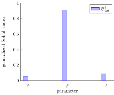
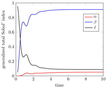
To illustrate the concepts introduced so far, we return to the mechanical oscillator example (3) and compute its generalized total Sobol’ indices; see Figure 2 (left). Figure 2 (right) illustrates the evolution of the generalized Sobol’ indices over successively larger intervals. These results provide a clear analysis of the relative importance of the input parameters along with a “history aware” description of the evolution of these relative importance measurements. While the pointwise in time Sobol’ indices show a significant growing influence of $\alpha$ over time, see again Figure 1(right), the generalized indices stabilize quickly and provide an importance assessment of the variables that is consistent over time.

Figure 2: Behavior of the mechanical oscillator problem (3) with uncertain parameters $\alpha\sim\mathcal{U}(3/8,5/8)$, $\beta\sim\mathcal{U}(10/4,15/4)$ and $\ell\sim\mathcal{U}(-5/4,-3/4)$. Left: generalized Sobol’ indices $\mathfrak{{S}}_{\text{tot}}^{U}(y;T)$, $U=\alpha,\beta,\ell$, with $T=10$ and $y$ is the solution to (3). Right: $\mathfrak{{S}}_{\text{tot}}^{U}(y;\tau)$ with $\tau\in(0,10)$.

3 A priori estimates with fixed unimportant variables

Suppose we have identified a subset ${{\mathchoice{\mbox{\boldmath$\displaystyle{\xi}$}}{\mbox{\boldmath$\textstyle{\xi}$}}{\mbox{\boldmath$\scriptstyle{\xi}$}}{\mbox{\boldmath$\scriptscriptstyle{\xi}$}}}_{U}}$, $U\subset X=\{1,\ldots,{N_{\text{p}}}\}$, of parameters such that $\mathfrak{{S}}_{\text{tot}}^{U^{\complement}}(f;T)$ is small compared to $\mathfrak{{S}}_{\text{tot}}^{U}$. In other words, the parameters ${{\mathchoice{\mbox{\boldmath$\displaystyle{\xi}$}}{\mbox{\boldmath$\textstyle{\xi}$}}{\mbox{\boldmath$\scriptstyle{\xi}$}}{\mbox{\boldmath$\scriptscriptstyle{\xi}$}}}_{U^{\complement}}}$ are unimportant and it should thus be possible to fix them at some nominal value ${\bar{\mathchoice{\mbox{\boldmath$\displaystyle{\xi}$}}{\mbox{\boldmath$\textstyle{\xi}$}}{\mbox{\boldmath$\scriptstyle{\xi}$}}{\mbox{\boldmath$\scriptscriptstyle{\xi}$}}}_{U^{\complement}}}$ and consider the “reduced” function

$$\bar{f}(t,{{\mathchoice{\mbox{\boldmath$\displaystyle{\xi}$}}{\mbox{\boldmath$\textstyle{\xi}$}}{\mbox{\boldmath$\scriptstyle{\xi}$}}{\mbox{\boldmath$\scriptscriptstyle{\xi}$}}}_{U}})=f(t,{{\mathchoice{\mbox{\boldmath$\displaystyle{\xi}$}}{\mbox{\boldmath$\textstyle{\xi}$}}{\mbox{\boldmath$\scriptstyle{\xi}$}}{\mbox{\boldmath$\scriptscriptstyle{\xi}$}}}_{U}},{\bar{\mathchoice{\mbox{\boldmath$\displaystyle{\xi}$}}{\mbox{\boldmath$\textstyle{\xi}$}}{\mbox{\boldmath$\scriptstyle{\xi}$}}{\mbox{\boldmath$\scriptscriptstyle{\xi}$}}}_{U^{\complement}}}),$$

as a reasonable approximation of $f$. The next result formalizes this line of thought by establishing a direct link between $\mathfrak{{S}}_{\text{tot}}^{{\mathchoice{\mbox{\boldmath$\displaystyle{\xi}$}}{\mbox{\boldmath$\textstyle{\xi}$}}{\mbox{\boldmath$\scriptstyle{\xi}$}}{\mbox{\boldmath$\scriptscriptstyle{\xi}$}}}_{U^{\complement}}}(f;T)$ and a measure of the relative error attached to the approximation $f\approx\bar{f}$; this result generalizes to time dependent problems the work of [30] on stationary problems.

Proposition 3.1.

Let $\mbox{\large$\varepsilon$}(f;t,{\bar{\mathchoice{\mbox{\boldmath$\displaystyle{\xi}$}}{\mbox{\boldmath$\textstyle{\xi}$}}{\mbox{\boldmath$\scriptstyle{\xi}$}}{\mbox{\boldmath$\scriptscriptstyle{\xi}$}}}_{U^{\complement}}})=\frac{1}{2}\int\left(f(t,{\mathchoice{\mbox{\boldmath$\displaystyle{\xi}$}}{\mbox{\boldmath$\textstyle{\xi}$}}{\mbox{\boldmath$\scriptstyle{\xi}$}}{\mbox{\boldmath$\scriptscriptstyle{\xi}$}}})-\bar{f}(t,{{\mathchoice{\mbox{\boldmath$\displaystyle{\xi}$}}{\mbox{\boldmath$\textstyle{\xi}$}}{\mbox{\boldmath$\scriptstyle{\xi}$}}{\mbox{\boldmath$\scriptscriptstyle{\xi}$}}}_{U}})\right)^{2}\,\mu(d{\mathchoice{\mbox{\boldmath$\displaystyle{\xi}$}}{\mbox{\boldmath$\textstyle{\xi}$}}{\mbox{\boldmath$\scriptstyle{\xi}$}}{\mbox{\boldmath$\scriptscriptstyle{\xi}$}}})$. Then

$$\mathscr{E}:=\frac{\int_{0}^{T}\mbox{\large$\varepsilon$}(f;t,{\bar{\mathchoice{\mbox{\boldmath$\displaystyle{\xi}$}}{\mbox{\boldmath$\textstyle{\xi}$}}{\mbox{\boldmath$\scriptstyle{\xi}$}}{\mbox{\boldmath$\scriptscriptstyle{\xi}$}}}_{U^{\complement}}})\,dt}{\int_{0}^{T}D(f;t)\,dt}$$

provides a measurement of the relative error linked to the approximation $f\approx\bar{f}$ and furthermore

$$\mathbb{E}\{\mathscr{E}\}=\mathfrak{{S}}_{\text{tot}}^{{\mathchoice{\mbox{\boldmath$\displaystyle{\xi}$}}{\mbox{\boldmath$\textstyle{\xi}$}}{\mbox{\boldmath$\scriptstyle{\xi}$}}{\mbox{\boldmath$\scriptscriptstyle{\xi}$}}}_{U^{\complement}}}(f;T).$$

Proof.

Let ${\Omega_{2}}=[-1,1]^{\text{dim}({{\mathchoice{\mbox{\boldmath$\displaystyle{\xi}$}}{\mbox{\boldmath$\textstyle{\xi}$}}{\mbox{\boldmath$\scriptstyle{\xi}$}}{\mbox{\boldmath$\scriptscriptstyle{\xi}$}}}_{U^{\complement}}})}$ where $\text{dim}({{\mathchoice{\mbox{\boldmath$\displaystyle{\xi}$}}{\mbox{\boldmath$\textstyle{\xi}$}}{\mbox{\boldmath$\scriptstyle{\xi}$}}{\mbox{\boldmath$\scriptscriptstyle{\xi}$}}}_{U^{\complement}}})$ denotes the dimension of ${{\mathchoice{\mbox{\boldmath$\displaystyle{\xi}$}}{\mbox{\boldmath$\textstyle{\xi}$}}{\mbox{\boldmath$\scriptstyle{\xi}$}}{\mbox{\boldmath$\scriptscriptstyle{\xi}$}}}_{U^{\complement}}}$, and let $\mu_{2}$ be the normalized Lebesgue measure on ${\Omega_{2}}$. We have

$$\mathbb{E}\left\{\int_{0}^{T}\mbox{\large$\varepsilon$}(f;t,{\bar{\mathchoice{\mbox{\boldmath$\displaystyle{\xi}$}}{\mbox{\boldmath$\textstyle{\xi}$}}{\mbox{\boldmath$\scriptstyle{\xi}$}}{\mbox{\boldmath$\scriptscriptstyle{\xi}$}}}_{U^{\complement}}})\,dt\right\}=\int_{\Omega_{2}}\int_{0}^{T}\mbox{\large$\varepsilon$}(f;t,{\bar{\mathchoice{\mbox{\boldmath$\displaystyle{\xi}$}}{\mbox{\boldmath$\textstyle{\xi}$}}{\mbox{\boldmath$\scriptstyle{\xi}$}}{\mbox{\boldmath$\scriptscriptstyle{\xi}$}}}_{U^{\complement}}})\,dt\,\mu_{2}(d{\bar{\mathchoice{\mbox{\boldmath$\displaystyle{\xi}$}}{\mbox{\boldmath$\textstyle{\xi}$}}{\mbox{\boldmath$\scriptstyle{\xi}$}}{\mbox{\boldmath$\scriptscriptstyle{\xi}$}}}_{U^{\complement}}})=\int_{0}^{T}\int_{\Omega_{2}}\mbox{\large$\varepsilon$}(f;t,{\bar{\mathchoice{\mbox{\boldmath$\displaystyle{\xi}$}}{\mbox{\boldmath$\textstyle{\xi}$}}{\mbox{\boldmath$\scriptstyle{\xi}$}}{\mbox{\boldmath$\scriptscriptstyle{\xi}$}}}_{U^{\complement}}})\,\mu_{2}(d{\bar{\mathchoice{\mbox{\boldmath$\displaystyle{\xi}$}}{\mbox{\boldmath$\textstyle{\xi}$}}{\mbox{\boldmath$\scriptstyle{\xi}$}}{\mbox{\boldmath$\scriptscriptstyle{\xi}$}}}_{U^{\complement}}})\,dt\\ =\int_{0}^{T}\mathbb{E}\{\mbox{\large$\varepsilon$}(f;t,{\bar{\mathchoice{\mbox{\boldmath$\displaystyle{\xi}$}}{\mbox{\boldmath$\textstyle{\xi}$}}{\mbox{\boldmath$\scriptstyle{\xi}$}}{\mbox{\boldmath$\scriptscriptstyle{\xi}$}}}_{U^{\complement}}})\}\,dt,$$

where the interchange of integrals follows from Tonelli’s theorem. Further, by the theorem proved in [30], $\mathbb{E}\{\mbox{\large$\varepsilon$}(f;t,{\bar{\mathchoice{\mbox{\boldmath$\displaystyle{\xi}$}}{\mbox{\boldmath$\textstyle{\xi}$}}{\mbox{\boldmath$\scriptstyle{\xi}$}}{\mbox{\boldmath$\scriptscriptstyle{\xi}$}}}_{U^{\complement}}})\}=D_{\text{tot}}^{U^{\complement}}(f;t)$ for each $t\in[0,T]$, and thus

$$\mathbb{E}\left\{\int_{0}^{T}\mbox{\large$\varepsilon$}(f;t,{\bar{\mathchoice{\mbox{\boldmath$\displaystyle{\xi}$}}{\mbox{\boldmath$\textstyle{\xi}$}}{\mbox{\boldmath$\scriptstyle{\xi}$}}{\mbox{\boldmath$\scriptscriptstyle{\xi}$}}}_{U^{\complement}}})\,dt\right\}=\int_{0}^{T}D_{\text{tot}}^{U^{\complement}}(f;t)\,dt.$$

This proves the result since $D(f;t)$ is deterministic. ∎

A more explicit probabilistic interpretation of Proposition 3.1 can be established by considering the quantity $\rho=\mathscr{E}/\mathfrak{{S}}_{\text{tot}}^{U^{\complement}}(f;T)$ and noting that $\mathbb{E}\{\rho\}=1$. As $\rho\geq 0$, the following result is a direct consequence of Markov’s inequality.

Corollary 3.2.

For every $\mbox{\large$\varepsilon$}>0$,

$$\mathbb{P}\Big{(}\mathscr{E}\geq\frac{1}{\mbox{\large$\varepsilon$}}\mathfrak{{S}}_{\text{tot}}^{U^{\complement}}(f;T)\Big{)}\leq\mbox{\large$\varepsilon$}.$$

4 Efficient computation of the sensitivity indices

4.1 Pointwise-in-time surrogate models

To alleviate the cost of computing the generalized Sobol’ indices, we can approximate $f(t,{\mathchoice{\mbox{\boldmath$\displaystyle{\xi}$}}{\mbox{\boldmath$\textstyle{\xi}$}}{\mbox{\boldmath$\scriptstyle{\xi}$}}{\mbox{\boldmath$\scriptscriptstyle{\xi}$}}})$ with a cheap-to-evaluate surrogate model $\tilde{f}(t,{\mathchoice{\mbox{\boldmath$\displaystyle{\xi}$}}{\mbox{\boldmath$\textstyle{\xi}$}}{\mbox{\boldmath$\scriptstyle{\xi}$}}{\mbox{\boldmath$\scriptscriptstyle{\xi}$}}})$, leading to the approximation

$$\mathfrak{{S}}^{U}(f;T)\approx\tilde{\mathfrak{{S}}}^{U}(f;T)=\frac{\int_{0}^{T}D^{U}(\tilde{f};t)\,dt}{\int_{0}^{T}D(\tilde{f};t)\,dt},$$ (16)

which can be computed at negligible cost. We outline the corresponding procedure in Algorithm 1. The main computational cost is the evaluations of the process $f$ at the sampling points $\{{\mathchoice{\mbox{\boldmath$\displaystyle{\xi}$}}{\mbox{\boldmath$\textstyle{\xi}$}}{\mbox{\boldmath$\scriptstyle{\xi}$}}{\mbox{\boldmath$\scriptscriptstyle{\xi}$}}}^{(j)}\}_{j=1}^{N}$. Once a surrogate model $\tilde{f}$ is available, the generalized Sobol’ index $\tilde{\mathfrak{{S}}}^{U}_{\text{tot}}(f;T)$ can be computed for any $U\subset\{1,\ldots,{N_{\text{p}}}\}$ using $\tilde{f}$.

Algorithm 1 Computation of the generalized Sobol’ indices via surrogate models constructed pointwise in time.

0:  (i) A quadrature formula on $[0,T]$ with nodes and weights $\{t_{m},w_{m}\}_{m=1}^{N_{\text{quad}}}$. (ii) function evaluations $\{f(t_{m},{\mathchoice{\mbox{\boldmath$\displaystyle{\xi}$}}{\mbox{\boldmath$\textstyle{\xi}$}}{\mbox{\boldmath$\scriptstyle{\xi}$}}{\mbox{\boldmath$\scriptscriptstyle{\xi}$}}}^{(j)})\}$, $m\in\{1,\ldots,{N_{\text{quad}}}\}$, $j\in\{1,\ldots,N\}$; (iii) An index set $U\subset\{1,\ldots,{N_{\text{p}}}\}$.

0:  Approximate generalized Sobol’ index $\tilde{\mathfrak{{S}}}^{U}_{\text{tot}}(f;T)$.

1:  Using the ensemble $\{f(t_{m},{\mathchoice{\mbox{\boldmath$\displaystyle{\xi}$}}{\mbox{\boldmath$\textstyle{\xi}$}}{\mbox{\boldmath$\scriptstyle{\xi}$}}{\mbox{\boldmath$\scriptscriptstyle{\xi}$}}}^{(j)})\}$, construct a surrogate model $\tilde{f}(t_{m},{\mathchoice{\mbox{\boldmath$\displaystyle{\xi}$}}{\mbox{\boldmath$\textstyle{\xi}$}}{\mbox{\boldmath$\scriptstyle{\xi}$}}{\mbox{\boldmath$\scriptscriptstyle{\xi}$}}})\approx f(t_{m},{\mathchoice{\mbox{\boldmath$\displaystyle{\xi}$}}{\mbox{\boldmath$\textstyle{\xi}$}}{\mbox{\boldmath$\scriptstyle{\xi}$}}{\mbox{\boldmath$\scriptscriptstyle{\xi}$}}})$, $m\in\{1,\ldots,{N_{\text{quad}}}\}$.

2:  Evaluate the approximate generalized Sobol’ index,

$$\tilde{\mathfrak{{S}}}^{U}(f;T)=\frac{\sum_{m=1}^{N_{\text{quad}}}w_{m}D^{U}(\tilde{f};t_{m})}{\sum_{m=1}^{N_{\text{quad}}}w_{m}D(\tilde{f};t_{m})}.$$

Polynomial chaos (PC) expansions are commonly used in surrogate modeling. We now elaborate on Algorithm 1 when using PC surrogates. PC expansions are series expansion of square integrable random variables in multivariate orthogonal polynomial bases [31, 11, 10]. The (truncated) PC representation of $f(t,{\mathchoice{\mbox{\boldmath$\displaystyle{\xi}$}}{\mbox{\boldmath$\textstyle{\xi}$}}{\mbox{\boldmath$\scriptstyle{\xi}$}}{\mbox{\boldmath$\scriptscriptstyle{\xi}$}}})$ is of the form

$$f(t,{\mathchoice{\mbox{\boldmath$\displaystyle{\xi}$}}{\mbox{\boldmath$\textstyle{\xi}$}}{\mbox{\boldmath$\scriptstyle{\xi}$}}{\mbox{\boldmath$\scriptscriptstyle{\xi}$}}})\approx\sum_{k=0}^{{N_{\text{PC}}}}c_{k}(t)\Psi_{k}({\mathchoice{\mbox{\boldmath$\displaystyle{\xi}$}}{\mbox{\boldmath$\textstyle{\xi}$}}{\mbox{\boldmath$\scriptstyle{\xi}$}}{\mbox{\boldmath$\scriptscriptstyle{\xi}$}}}),$$ (17)

where $\{\Psi_{k}\}_{k=0}^{N_{\text{PC}}}$ is a set of orthogonal polynomials and $\{c_{k}\}_{k=0}^{N_{\text{PC}}}$ are expansion coefficients. As $\textstyle{\xi}$ is assumed to be a ${N_{\text{p}}}$-dimensional uniform random vector, we choose ${N_{\text{p}}}$-variate Legendre polynomials for $\{\Psi_{k}\}_{k=0}^{N_{\text{PC}}}$; see [10]. Also, we use total order truncation [10] and thus

$${N_{\text{PC}}}+1=\frac{\left({N_{\text{ord}}}+{N_{\text{p}}}\right)!}{{N_{\text{ord}}}!{N_{\text{p}}}!},$$ (18)

where ${N_{\text{ord}}}$ is the maximum total polynomial degree. The following are two common approaches for computing PC coefficients via sampling; i.e., in a non-intrusive way

• Non-intrusive spectral projection (NISP),

• Regression based methods with sparsity control.

Let $u\in L^{2}_{\mu}(\Omega)=\{u:\Omega\to\mathbb{R}:\int_{\Omega}u(x)^{2}\mu(dx)<\infty\}$ to be approximated through the PC representation

$$u\approx\sum_{i=0}^{N_{\text{PC}}}c_{k}\Psi_{k}.$$

The NISP approach [10, 32, 33, 34, 35], is based on the approximation of Galerkin projections

$$\langle{u},{\Psi_{l}}\rangle=\int u({\mathchoice{\mbox{\boldmath$\displaystyle{\xi}$}}{\mbox{\boldmath$\textstyle{\xi}$}}{\mbox{\boldmath$\scriptstyle{\xi}$}}{\mbox{\boldmath$\scriptscriptstyle{\xi}$}}})\Psi_{l}({\mathchoice{\mbox{\boldmath$\displaystyle{\xi}$}}{\mbox{\boldmath$\textstyle{\xi}$}}{\mbox{\boldmath$\scriptstyle{\xi}$}}{\mbox{\boldmath$\scriptscriptstyle{\xi}$}}})\mu(d{\mathchoice{\mbox{\boldmath$\displaystyle{\xi}$}}{\mbox{\boldmath$\textstyle{\xi}$}}{\mbox{\boldmath$\scriptstyle{\xi}$}}{\mbox{\boldmath$\scriptscriptstyle{\xi}$}}})=\sum_{k=0}^{{N_{\text{PC}}}}\int c_{k}\Psi_{k}({\mathchoice{\mbox{\boldmath$\displaystyle{\xi}$}}{\mbox{\boldmath$\textstyle{\xi}$}}{\mbox{\boldmath$\scriptstyle{\xi}$}}{\mbox{\boldmath$\scriptscriptstyle{\xi}$}}})\Psi_{l}({\mathchoice{\mbox{\boldmath$\displaystyle{\xi}$}}{\mbox{\boldmath$\textstyle{\xi}$}}{\mbox{\boldmath$\scriptstyle{\xi}$}}{\mbox{\boldmath$\scriptscriptstyle{\xi}$}}})\,\mu(d{\mathchoice{\mbox{\boldmath$\displaystyle{\xi}$}}{\mbox{\boldmath$\textstyle{\xi}$}}{\mbox{\boldmath$\scriptstyle{\xi}$}}{\mbox{\boldmath$\scriptscriptstyle{\xi}$}}})\\ =\sum_{k=0}^{{N_{\text{PC}}}}c_{k}\langle{\Psi_{k}},{\Psi_{l}}\rangle=c_{l}\langle{\Psi_{l}},{\Psi_{l}}\rangle.$$

through quadrature

$$\langle{u},{\Psi_{l}}\rangle\approx\sum_{j=1}^{{N_{\text{quad}}^{\text{nisp}}}}\nu_{j}u\big{(}{\mathchoice{\mbox{\boldmath$\displaystyle{\xi}$}}{\mbox{\boldmath$\textstyle{\xi}$}}{\mbox{\boldmath$\scriptstyle{\xi}$}}{\mbox{\boldmath$\scriptscriptstyle{\xi}$}}}^{(j)}\big{)}\Psi_{l}\big{(}{\mathchoice{\mbox{\boldmath$\displaystyle{\xi}$}}{\mbox{\boldmath$\textstyle{\xi}$}}{\mbox{\boldmath$\scriptstyle{\xi}$}}{\mbox{\boldmath$\scriptscriptstyle{\xi}$}}}^{(j)}\big{)}.$$ (19)

Here ${\mathchoice{\mbox{\boldmath$\displaystyle{\xi}$}}{\mbox{\boldmath$\textstyle{\xi}$}}{\mbox{\boldmath$\scriptstyle{\xi}$}}{\mbox{\boldmath$\scriptscriptstyle{\xi}$}}}^{(j)}\in\Omega$ and $\nu_{j}\geq 0$, $j\in\{1,\ldots,{N_{\text{quad}}^{\text{nisp}}}\}$, are quadrature nodes and weights.

Alternatively, PC coefficients can be computed through regression-based approaches. Borrowing ideas from compressive sensing (CS), sparsity is enforced by controlling the $\ell_{1}$ norm of the vector of PC coefficients. We refer to this as the CS-based approach. This approach has been used extensively in recent years for efficient computation of PC expansions, see e.g., [36, 37, 38, 39].

We explain a common formulation of a CS-based approach. We begin by forming a sample of points $\{{\mathchoice{\mbox{\boldmath$\displaystyle{\xi}$}}{\mbox{\boldmath$\textstyle{\xi}$}}{\mbox{\boldmath$\scriptstyle{\xi}$}}{\mbox{\boldmath$\scriptscriptstyle{\xi}$}}}^{(j)}\}_{j=1}^{N}$ in the sample space $\Omega$ and let $\mathbf{\Lambda}\in\mathbb{R}^{N\times{N_{\text{PC}}}}$ be defined by $\Lambda_{jk}=\Psi_{k}({\mathchoice{\mbox{\boldmath$\displaystyle{\xi}$}}{\mbox{\boldmath$\textstyle{\xi}$}}{\mbox{\boldmath$\scriptstyle{\xi}$}}{\mbox{\boldmath$\scriptscriptstyle{\xi}$}}}^{(j)})$, and ${\mathchoice{\mbox{\boldmath$\displaystyle{d}$}}{\mbox{\boldmath$\textstyle{d}$}}{\mbox{\boldmath$\scriptstyle{d}$}}{\mbox{\boldmath$\scriptscriptstyle{d}$}}}=\big{(}u({\mathchoice{\mbox{\boldmath$\displaystyle{\xi}$}}{\mbox{\boldmath$\textstyle{\xi}$}}{\mbox{\boldmath$\scriptstyle{\xi}$}}{\mbox{\boldmath$\scriptscriptstyle{\xi}$}}}^{(1)}),\ldots,u({\mathchoice{\mbox{\boldmath$\displaystyle{\xi}$}}{\mbox{\boldmath$\textstyle{\xi}$}}{\mbox{\boldmath$\scriptstyle{\xi}$}}{\mbox{\boldmath$\scriptscriptstyle{\xi}$}}}^{(N)})\big{)}^{\mkern-1.5mu\mathsf{T}}$ be the vector that contains the function evaluations. The vector of PC coefficients is then determined by solving

$$\min_{{\mathchoice{\mbox{\boldmath$\displaystyle{c}$}}{\mbox{\boldmath$\textstyle{c}$}}{\mbox{\boldmath$\scriptstyle{c}$}}{\mbox{\boldmath$\scriptscriptstyle{c}$}}}\in\mathbb{R}^{{N_{\text{PC}}}}}\|\mathbf{\Lambda}{\mathchoice{\mbox{\boldmath$\displaystyle{c}$}}{\mbox{\boldmath$\textstyle{c}$}}{\mbox{\boldmath$\scriptstyle{c}$}}{\mbox{\boldmath$\scriptscriptstyle{c}$}}}-{\mathchoice{\mbox{\boldmath$\displaystyle{d}$}}{\mbox{\boldmath$\textstyle{d}$}}{\mbox{\boldmath$\scriptstyle{d}$}}{\mbox{\boldmath$\scriptscriptstyle{d}$}}}\|_{2}^{2},\quad\text{subject to }\sum_{k=0}^{N_{\text{PC}}}|c_{k}|\leq\tau.$$ (20)

In our computations, we use the solver SPGL1 [40] for the optimization problem (20). The parameter $\tau$ that controls the sparsity of $c$ is found either by trial and error or, more systematically, through a cross validation procedure.

Consider now the PC representation $f(t,{\mathchoice{\mbox{\boldmath$\displaystyle{\xi}$}}{\mbox{\boldmath$\textstyle{\xi}$}}{\mbox{\boldmath$\scriptstyle{\xi}$}}{\mbox{\boldmath$\scriptscriptstyle{\xi}$}}})\approx\sum_{k=0}^{N_{\text{PC}}}c_{k}(t)\Psi_{k}({\mathchoice{\mbox{\boldmath$\displaystyle{\xi}$}}{\mbox{\boldmath$\textstyle{\xi}$}}{\mbox{\boldmath$\scriptstyle{\xi}$}}{\mbox{\boldmath$\scriptscriptstyle{\xi}$}}})$. We have

$$\mathfrak{{S}}_{\text{tot}}^{i}(f;T)=\frac{\int_{0}^{T}D_{\text{tot}}^{i}(f;t)\,dt}{\int_{0}^{T}D(f;t)\,dt}\approx\frac{\displaystyle\sum_{k\in\mathcal{K}_{i}}\|\Psi_{k}\|^{2}\int_{0}^{T}c_{k}(t)^{2}\,dt}{\displaystyle\sum_{k=1}^{N_{\text{PC}}}\|\Psi_{k}\|^{2}\int_{0}^{T}c_{k}(t)^{2}\,dt},\quad i\in\{1,\ldots,{N_{\text{p}}}\}.$$ (21)

Here $\mathcal{K}_{i}$ is an index set that picks all the terms in the PC expansion that include $\xi_{i}$. The definition of this index set is facilitated by the (partial) tensor product construction of PC basis functions [14, 13, 16, 5]; see A for a brief description. Note that (21) corresponds to $\mathfrak{{S}}_{\text{tot}}^{U}(f;T)$ with $U=\{i\}$, $i\in\{1,\ldots,{N_{\text{p}}}\}$. It is straightforward to generalize the expression for arbitrary $U\subset\{1,\ldots,{N_{\text{p}}}\}$.

The integrals in (21) are computed numerically using a quadrature formula on $[0,T]$ with nodes and weights $\{t_{m},w_{m}\}_{m=1}^{N_{\text{quad}}}$. This requires computing PC coefficients at every $t_{m}$, $m\in\{1,\ldots,{N_{\text{quad}}}\}$. The NISP and CS-based approaches for computing PC representation of $f(t,{\mathchoice{\mbox{\boldmath$\displaystyle{\xi}$}}{\mbox{\boldmath$\textstyle{\xi}$}}{\mbox{\boldmath$\scriptstyle{\xi}$}}{\mbox{\boldmath$\scriptscriptstyle{\xi}$}}})$ share a common feature: a set of function evaluations $f(t_{m},{\mathchoice{\mbox{\boldmath$\displaystyle{\xi}$}}{\mbox{\boldmath$\textstyle{\xi}$}}{\mbox{\boldmath$\scriptstyle{\xi}$}}{\mbox{\boldmath$\scriptscriptstyle{\xi}$}}}^{(j)})$, $j\in\{1,\ldots,N\}$, $m\in\{1,\ldots,{N_{\text{quad}}}\}$ is needed. This is the main computational bottleneck for both methods.

With NISP, the sampling points are chosen according to a quadrature rule. The CS-based approach, on the other hand, offers more flexibility and allows for Monte Carlo or quasi Monte Carlo sampling. The computational cost of the NISP numerical quadratures can be very high, especially with full tensorization of one-dimensional quadrature rules and/or when the parameter dimension is large. The computational cost can be reduced by carrying out the integration in (19) through Smolyak sparse quadrature [41, 42]. A common restriction of both the NISP and CS-based approaches is the need to access the same set of sampling points for each $t\in\{t_{1},\ldots,t_{N_{\text{quad}}}\}$. While changing the sampling points for each time could lead to better approximations, especially if adaptive quadrature-based approaches are used [34, 35], the number of required function evaluations would be prohibitive.

Algorithm 2 PC-NISP approach for computation of the generalized Sobol’ indices

0:  (i) A quadrature formula on $[0,T]$ with nodes and weights $\{t_{m},w_{m}\}_{m=1}^{N_{\text{quad}}}$. (ii) a quadrature formula on $\Omega$ with nodes and weights $\{{\mathchoice{\mbox{\boldmath$\displaystyle{\xi}$}}{\mbox{\boldmath$\textstyle{\xi}$}}{\mbox{\boldmath$\scriptstyle{\xi}$}}{\mbox{\boldmath$\scriptscriptstyle{\xi}$}}}^{(j)},\nu_{j}\}_{j=1}^{N_{\text{quad}}^{\text{nisp}}}$; (iii) function evaluations $\{f(t_{m},{\mathchoice{\mbox{\boldmath$\displaystyle{\xi}$}}{\mbox{\boldmath$\textstyle{\xi}$}}{\mbox{\boldmath$\scriptstyle{\xi}$}}{\mbox{\boldmath$\scriptscriptstyle{\xi}$}}}^{(j)})\}$, $m\in\{1,\ldots,{N_{\text{quad}}}\}$, $j\in\{1,\ldots,{N_{\text{quad}}^{\text{nisp}}}\}$; (iv) a PC basis $\{\Psi_{k}\}_{k=0}^{N_{\text{PC}}}$.

0:  Approximate generalized total Indices $\tilde{\mathfrak{{S}}}^{i}_{\text{tot}}(f;T)$, $i\in\{1,\ldots,{N_{\text{p}}}\}$.

1:  Form the projection matrix

$$\Pi_{kj}=\nu_{j}\Psi_{k}({\mathchoice{\mbox{\boldmath$\displaystyle{\xi}$}}{\mbox{\boldmath$\textstyle{\xi}$}}{\mbox{\boldmath$\scriptstyle{\xi}$}}{\mbox{\boldmath$\scriptscriptstyle{\xi}$}}}^{(j)})/\langle{\Psi_{k}},{\Psi_{k}}\rangle,\quad k\in\{0,\ldots,{N_{\text{PC}}}\},\,j\in\{1,\ldots,{N_{\text{quad}}^{\text{nisp}}}\}$$

2:  Compute the vector of PC coefficients at each time step:

$${\mathchoice{\mbox{\boldmath$\displaystyle{c}$}}{\mbox{\boldmath$\textstyle{c}$}}{\mbox{\boldmath$\scriptstyle{c}$}}{\mbox{\boldmath$\scriptscriptstyle{c}$}}}(t_{m})=\mathbf{\Pi}{\mathchoice{\mbox{\boldmath$\displaystyle{d}$}}{\mbox{\boldmath$\textstyle{d}$}}{\mbox{\boldmath$\scriptstyle{d}$}}{\mbox{\boldmath$\scriptscriptstyle{d}$}}}(t_{m}),\quad m\in\{1,\ldots,{N_{\text{quad}}}\}.$$

3:  Compute approximations to the generalized total sensitivity indices according to (21):

$$\tilde{\mathfrak{{S}}}^{i}_{\text{tot}}(f;T)=\frac{\displaystyle\sum_{k\in\mathcal{K}_{i}}\sum_{m=1}^{N_{\text{quad}}}\|\Psi_{k}\|^{2}w_{m}c_{k}(t_{m})^{2}}{\displaystyle\sum_{k=1}^{N_{\text{kl}}}\sum_{m=1}^{N_{\text{quad}}}\|\Psi_{k}\|^{2}w_{m}c_{k}(t_{m})^{2}}.$$

To summarize, NISP is a convenient-to-implement approach for computing the time-dependent PC coefficients and consequently the generalized Sobol’ indices, and can be very effective for certain classes of problems. We outline the required steps in Algorithm 2.

Compared to NISP, CS-based methods present two additional challenges in the above context: (i) an optimization problem of the form (20) has to be solved at every $t_{m}$, $m\in\{1,\ldots,{N_{\text{quad}}}\}$ which can be prohibitive when ${N_{\text{quad}}}$ is large and (ii) the sparsity control parameter $\tau$ may need to be calibrated for each $t_{m}$. CS-based approaches for the joint sparse recovery of function-valued quantities of interest (such as time-dependent processes) have been proposed; they may provide viable alternatives to a pointwise-in-time CS-based strategy; see [43] and the references therein.

While PC expansions are widely applicable, they present known shortcomings for certain classes of time-dependent problems; see e.g., [44, 32, 45, 46, 47] that address problems where straightforward implementation of a PC-based approach is not optimal. Depending on the application at hand, other types of surrogates might provide better alternatives for the purposes of Algorithm 1.

4.2 The spectral approach

Even though the approach outlined in Section 4.1 can be effective; it makes no attempt at exploiting the structure of the problem. For instance, and as alluded to in the Introduction, computing a KL decomposition often reveals a low-rank representation. For such cases, the essential features of the corresponding time-dependent processes are captured with only a few dominant KL modes. Using such a representation, we can efficiently compute generalized Sobol’ indices, without the need for surrogate models at every point in time. This is the essence of the spectral approach.

Under the notation and assumptions of Section 2, we represent the process $f$ using the KL expansion

$$f(t,{\mathchoice{\mbox{\boldmath$\displaystyle{\xi}$}}{\mbox{\boldmath$\textstyle{\xi}$}}{\mbox{\boldmath$\scriptstyle{\xi}$}}{\mbox{\boldmath$\scriptscriptstyle{\xi}$}}})=\sum_{i=1}^{\infty}f_{i}({\mathchoice{\mbox{\boldmath$\displaystyle{\xi}$}}{\mbox{\boldmath$\textstyle{\xi}$}}{\mbox{\boldmath$\scriptstyle{\xi}$}}{\mbox{\boldmath$\scriptscriptstyle{\xi}$}}})e_{i}(t),\quad f_{i}({\mathchoice{\mbox{\boldmath$\displaystyle{\xi}$}}{\mbox{\boldmath$\textstyle{\xi}$}}{\mbox{\boldmath$\scriptstyle{\xi}$}}{\mbox{\boldmath$\scriptscriptstyle{\xi}$}}})=\int_{0}^{T}f(t,{\mathchoice{\mbox{\boldmath$\displaystyle{\xi}$}}{\mbox{\boldmath$\textstyle{\xi}$}}{\mbox{\boldmath$\scriptstyle{\xi}$}}{\mbox{\boldmath$\scriptscriptstyle{\xi}$}}})e_{i}(t)\,dt.$$ (22)

In practical computations, the above expansion is truncated

$$f^{({{N_{\text{kl}}}})}(t,{\mathchoice{\mbox{\boldmath$\displaystyle{\xi}$}}{\mbox{\boldmath$\textstyle{\xi}$}}{\mbox{\boldmath$\scriptstyle{\xi}$}}{\mbox{\boldmath$\scriptscriptstyle{\xi}$}}})=\sum_{i=1}^{N_{\text{kl}}}f_{i}({\mathchoice{\mbox{\boldmath$\displaystyle{\xi}$}}{\mbox{\boldmath$\textstyle{\xi}$}}{\mbox{\boldmath$\scriptstyle{\xi}$}}{\mbox{\boldmath$\scriptscriptstyle{\xi}$}}})e_{i}(t),$$

with the truncation level ${N_{\text{kl}}}$ being informed by the decay of the eigenvalues of $\mathcal{C}$. More precisely, as the variance of the truncated KL expansion is given by $\mathbb{V}\left\{{f^{({{N_{\text{kl}}}})}(t,{\mathchoice{\mbox{\boldmath$\displaystyle{\xi}$}}{\mbox{\boldmath$\textstyle{\xi}$}}{\mbox{\boldmath$\scriptstyle{\xi}$}}{\mbox{\boldmath$\scriptscriptstyle{\xi}$}}})}\right\}=\sum_{i=1}^{N_{\text{kl}}}\lambda_{i}e_{i}(t)^{2}$ (cf. Lemma 1(2) in B) it is possible to adjust the truncation level ${N_{\text{kl}}}$ by considering the fraction $r_{N_{\text{kl}}}$ of the variance quantified by a given truncation level:

$$r_{N_{\text{kl}}}=\frac{\int_{0}^{T}\mathbb{V}\left\{{f^{({{N_{\text{kl}}}})}(t,{\mathchoice{\mbox{\boldmath$\displaystyle{\xi}$}}{\mbox{\boldmath$\textstyle{\xi}$}}{\mbox{\boldmath$\scriptstyle{\xi}$}}{\mbox{\boldmath$\scriptscriptstyle{\xi}$}}})}\right\}\,dt}{\int_{0}^{T}\mathbb{V}\left\{{f(t,{\mathchoice{\mbox{\boldmath$\displaystyle{\xi}$}}{\mbox{\boldmath$\textstyle{\xi}$}}{\mbox{\boldmath$\scriptstyle{\xi}$}}{\mbox{\boldmath$\scriptscriptstyle{\xi}$}}})}\right\}\,dt}=\frac{\sum_{i=1}^{N_{\text{kl}}}\lambda_{i}}{\sum_{i=1}^{\infty}\lambda_{i}}.$$ (23)

A similar criterion is used in the computational fluid dynamics community when truncating proper orthogonal decompositions (POD) for reduced order modeling [48]. The rate at which the eigenvalues of the covariance operator $\mathcal{C}$ decay is problem-dependent. There are, however, many applications of interest, where the process $f$ corresponds to a dynamical system with uncertain parameters, for which a small number of KL modes suffice. We call such processes low-rank.

Figure 3: Spectral properties of the mechanical oscillator problem (3). Left: eigenvalues of the covariance operator; middle: pointwise variance of $f^{({{N_{\text{kl}}}})}(t,{\mathchoice{\mbox{\boldmath$\displaystyle{\xi}$}}{\mbox{\boldmath$\textstyle{\xi}$}}{\mbox{\boldmath$\scriptstyle{\xi}$}}{\mbox{\boldmath$\scriptscriptstyle{\xi}$}}})$ for a few choices of ${N_{\text{kl}}}$; right: the ratio (23).

Figure 3 illustrates the spectral properties of the mechanical oscillator (3). The decay of the first $20$ normalized eigenvalues of the covariance operator is displayed in Figure 3 (left); the rapid decay observed there indicates that a few KL modes should provide a suitable representation for the process. For further insight, we show the evolution of the pointwise variance of $f^{({{N_{\text{kl}}}})}(t,{\mathchoice{\mbox{\boldmath$\displaystyle{\xi}$}}{\mbox{\boldmath$\textstyle{\xi}$}}{\mbox{\boldmath$\scriptstyle{\xi}$}}{\mbox{\boldmath$\scriptscriptstyle{\xi}$}}})$ for various values of ${N_{\text{kl}}}$ (Figure 3, middle) and the behavior of the ratio (23) for an increasing number of KL modes (Figure 3 right). The process corresponding to the oscillator problem is an example of a low-rank process. These results are obtained by approximating the covariance function according to (7) with a Monte Carlo sample of size $10^{4}$.

Spectral representations can be leveraged to yield efficient algorithms for the computation of the generalized Sobol’ indices. We present the following result that makes a direct link between the KL expansion of $f$ and the generalized Sobol indices.

Theorem 4.1.

Let $f$ be a centered process satisfying the assumptions of Section 2 together with its KL expansion from (22). Then, for $U\subset\{1,\ldots,{N_{\text{p}}}\}$,

$$\mathfrak{{S}}^{U}(f;T)=\frac{\sum_{i=1}^{\infty}\mathbb{V}\left\{{\mathbb{E}\left\{{f_{i}({\mathchoice{\mbox{\boldmath$\displaystyle{\xi}$}}{\mbox{\boldmath$\textstyle{\xi}$}}{\mbox{\boldmath$\scriptstyle{\xi}$}}{\mbox{\boldmath$\scriptscriptstyle{\xi}$}}})|{\mathchoice{\mbox{\boldmath$\displaystyle{\xi}$}}{\mbox{\boldmath$\textstyle{\xi}$}}{\mbox{\boldmath$\scriptstyle{\xi}$}}{\mbox{\boldmath$\scriptscriptstyle{\xi}$}}}_{U}}\right\}}\right\}}{\sum_{i=1}^{\infty}\lambda_{i}},$$ (24)

where $\lambda_{i}$ are eigenvalues of the covariance operator $\mathcal{C}$ corresponding to the process $f$.

Proof.

See B. ∎

Theorem 4.1 yields an efficient approach for numerically approximating the generalized Sobol’ indices in problems where the eigenvalues of the covariance operator exhibit rapid spectral decay; i.e., for low-rank processes. In such problems, we can obtain accurate approximations to the generalized sensitivity indices with only a few modes in the KL expansion. Then, focusing on the expression for $\mathfrak{{S}}^{U}(f;T)$, we consider building surrogate models for the individual modes $f_{i}({\mathchoice{\mbox{\boldmath$\displaystyle{\xi}$}}{\mbox{\boldmath$\textstyle{\xi}$}}{\mbox{\boldmath$\scriptstyle{\xi}$}}{\mbox{\boldmath$\scriptscriptstyle{\xi}$}}})$; using these, the variances $\mathbb{V}\left\{{\mathbb{E}\left\{{f_{i}({\mathchoice{\mbox{\boldmath$\displaystyle{\xi}$}}{\mbox{\boldmath$\textstyle{\xi}$}}{\mbox{\boldmath$\scriptstyle{\xi}$}}{\mbox{\boldmath$\scriptscriptstyle{\xi}$}}})|{\mathchoice{\mbox{\boldmath$\displaystyle{\xi}$}}{\mbox{\boldmath$\textstyle{\xi}$}}{\mbox{\boldmath$\scriptstyle{\xi}$}}{\mbox{\boldmath$\scriptscriptstyle{\xi}$}}}_{U}}\right\}}\right\}$ can be approximated efficiently.

From the approximate covariance function $c^{N}(s,t)$ in (7), we construct the following approximation of the covariance operator (10):

$$\mathcal{C}^{N}[u](s)=\int_{0}^{T}c^{N}(s,t)u(t)\,dt,\quad u\in L^{2}([0,T]).$$

This operator is then discretized using a quadrature formula in the interval $[0,T]$ with nodes and weights $t_{m}$, $w_{m}$, $m\in\{1,\ldots,{N_{\text{quad}}}\}$. To compute the spectral decomposition of $\mathcal{C}^{N}$ numerically, we have to solve the discretized (generalized) eigenvalue problem

$$\sum_{m=1}^{N_{\text{quad}}}w_{m}c^{N}(s_{l},t_{m})e_{i}(t_{m})=\lambda_{i}e_{i}(s_{l}),\quad l\in\{1,\ldots,{N_{\text{quad}}}\}.$$

Letting $e_{i}^{l}=e_{i}(t_{l})$, $K_{lm}=c^{N}(s_{l},t_{m})$, $l,m\in\{1,\ldots,{N_{\text{quad}}}\}$, and defining the matrix $\mathbf{W}=\operatorname{diag}(w_{1},w_{2},\ldots,w_{n})$, the discretized eigenvalue problem is given by

$$\mathbf{K}\mathbf{W}\mathbf{e}_{i}=\lambda_{i}\mathbf{e}_{i},\quad i\in\{1,2,\ldots,{N_{\text{quad}}}\}.$$

This can be rewritten in symmetric form

$$\mathbf{W}^{1/2}\mathbf{K}\mathbf{W}^{1/2}\mathbf{u}_{i}=\lambda_{i}\mathbf{u}_{i},\quad i\in\{1,2,\ldots,{N_{\text{quad}}}\},$$ (25)

with $\mathbf{u}_{i}=\mathbf{W}^{1/2}\mathbf{e}_{i}$. Solving this reformulated eigenvalue problem yields eigenvalues $\lambda_{i}$ and eigenvectors $\mathbf{e}_{i}=\mathbf{W}^{-1/2}\mathbf{u}_{i}$ that satisfy

$$\mathbf{e}_{i}^{\mkern-1.5mu\mathsf{T}}\mathbf{W}\mathbf{e}_{j}=\mathbf{u}_{i}^{\mkern-1.5mu\mathsf{T}}\mathbf{W}^{-1/2}\mathbf{W}\mathbf{W}^{-1/2}\mathbf{u}_{j}=\mathbf{u}_{i}^{\mkern-1.5mu\mathsf{T}}\mathbf{u}_{j}=\delta_{ij},\quad i,j\in\{1,\ldots,{N_{\text{quad}}}\}.$$

The present approach for computing the eigenvalues and eigenvectors of the covariance operator is known as the Nyström’s method.

Algorithm 3 Spectral-KL approach for computing the generalized total Sobol’ indices

0:  (i) A quadrature formula on $[0,T]$ with nodes and weights $\{t_{m},w_{m}\}_{m=1}^{N_{\text{quad}}}$. (ii) Function evaluations $\{f(t_{m},{\mathchoice{\mbox{\boldmath$\displaystyle{\xi}$}}{\mbox{\boldmath$\textstyle{\xi}$}}{\mbox{\boldmath$\scriptstyle{\xi}$}}{\mbox{\boldmath$\scriptscriptstyle{\xi}$}}}^{k})\}$, $l\in\{1,\ldots,{N_{\text{quad}}}\}$, $k\in\{1,\ldots,N\}$. (iii) An index set $U\subset\{1,\ldots,P\}$.

0:  Generalized Sobol’ index $\mathfrak{{S}}^{U}(f;T)$.

1:  Center the process

$$f_{c}(t_{m},{\mathchoice{\mbox{\boldmath$\displaystyle{\xi}$}}{\mbox{\boldmath$\textstyle{\xi}$}}{\mbox{\boldmath$\scriptstyle{\xi}$}}{\mbox{\boldmath$\scriptscriptstyle{\xi}$}}}^{k})=f(t_{m},{\mathchoice{\mbox{\boldmath$\displaystyle{\xi}$}}{\mbox{\boldmath$\textstyle{\xi}$}}{\mbox{\boldmath$\scriptstyle{\xi}$}}{\mbox{\boldmath$\scriptscriptstyle{\xi}$}}}^{k})-\frac{1}{N}\sum_{j=1}^{N}f(t_{m},{\mathchoice{\mbox{\boldmath$\displaystyle{\xi}$}}{\mbox{\boldmath$\textstyle{\xi}$}}{\mbox{\boldmath$\scriptstyle{\xi}$}}{\mbox{\boldmath$\scriptscriptstyle{\xi}$}}}^{j}),\quad k\in\{1,\ldots,N\},m\in\{1,\ldots,{N_{\text{quad}}}\}.$$

2:  Form covariance matrix (discretized covariance function)

$$K_{lm}=\frac{1}{N-1}\sum_{k=1}^{N}f_{c}(t_{l},{\mathchoice{\mbox{\boldmath$\displaystyle{\xi}$}}{\mbox{\boldmath$\textstyle{\xi}$}}{\mbox{\boldmath$\scriptstyle{\xi}$}}{\mbox{\boldmath$\scriptscriptstyle{\xi}$}}}^{k})f_{c}(t_{m},{\mathchoice{\mbox{\boldmath$\displaystyle{\xi}$}}{\mbox{\boldmath$\textstyle{\xi}$}}{\mbox{\boldmath$\scriptstyle{\xi}$}}{\mbox{\boldmath$\scriptscriptstyle{\xi}$}}}^{k}),\quad l,m\in\{1,\ldots,{N_{\text{quad}}}\}.$$

3:  Let $\mathbf{W}=\mathrm{diag}(w_{1},w_{2},\ldots,w_{N_{\text{quad}}})$ and solve the eigenvalue problem

$$\mathbf{W}^{1/2}\mathbf{K}\mathbf{W}^{1/2}\mathbf{u}_{i}=\lambda_{i}\mathbf{u}_{i},\quad i\in\{1,\ldots,{N_{\text{quad}}}\}.$$

4:  Compute $\mathbf{e}_{i}=\mathbf{W}^{-1/2}\mathbf{u}_{i}$, $i\in\{1,\ldots,{N_{\text{quad}}}\}$.

5:  Choose a truncation level ${N_{\text{kl}}}$, and compute the discretized KL modes,

$${f}_{i}({\mathchoice{\mbox{\boldmath$\displaystyle{\xi}$}}{\mbox{\boldmath$\textstyle{\xi}$}}{\mbox{\boldmath$\scriptstyle{\xi}$}}{\mbox{\boldmath$\scriptscriptstyle{\xi}$}}}^{k})=\sum_{m=1}^{N_{\text{quad}}}w_{m}f_{c}(t_{m},{\mathchoice{\mbox{\boldmath$\displaystyle{\xi}$}}{\mbox{\boldmath$\textstyle{\xi}$}}{\mbox{\boldmath$\scriptstyle{\xi}$}}{\mbox{\boldmath$\scriptscriptstyle{\xi}$}}}^{k})e_{i}^{m},\quad i\in\{1,\ldots,{N_{\text{kl}}}\},\,k\in\{1,\ldots,N\}.$$

6:  Compute a surrogate model for each $f_{i}$, using function evaluations $\{f_{i}({\mathchoice{\mbox{\boldmath$\displaystyle{\xi}$}}{\mbox{\boldmath$\textstyle{\xi}$}}{\mbox{\boldmath$\scriptstyle{\xi}$}}{\mbox{\boldmath$\scriptscriptstyle{\xi}$}}}^{k})\}_{k=1}^{N}$:

$$f_{i}({\mathchoice{\mbox{\boldmath$\displaystyle{\xi}$}}{\mbox{\boldmath$\textstyle{\xi}$}}{\mbox{\boldmath$\scriptstyle{\xi}$}}{\mbox{\boldmath$\scriptscriptstyle{\xi}$}}})\approx\tilde{f}_{i}({\mathchoice{\mbox{\boldmath$\displaystyle{\xi}$}}{\mbox{\boldmath$\textstyle{\xi}$}}{\mbox{\boldmath$\scriptstyle{\xi}$}}{\mbox{\boldmath$\scriptscriptstyle{\xi}$}}};{\mathchoice{\mbox{\boldmath$\displaystyle{\xi}$}}{\mbox{\boldmath$\textstyle{\xi}$}}{\mbox{\boldmath$\scriptstyle{\xi}$}}{\mbox{\boldmath$\scriptscriptstyle{\xi}$}}}^{1},{\mathchoice{\mbox{\boldmath$\displaystyle{\xi}$}}{\mbox{\boldmath$\textstyle{\xi}$}}{\mbox{\boldmath$\scriptstyle{\xi}$}}{\mbox{\boldmath$\scriptscriptstyle{\xi}$}}}^{2},\ldots,{\mathchoice{\mbox{\boldmath$\displaystyle{\xi}$}}{\mbox{\boldmath$\textstyle{\xi}$}}{\mbox{\boldmath$\scriptstyle{\xi}$}}{\mbox{\boldmath$\scriptscriptstyle{\xi}$}}}^{N}).$$

7:  Compute

$$\tilde{\mathfrak{{S}}}^{U}(f;T)=\frac{\sum_{i=1}^{N_{\text{kl}}}\mathbb{V}\left\{{\mathbb{E}\left\{{\tilde{f}_{i}({\mathchoice{\mbox{\boldmath$\displaystyle{\xi}$}}{\mbox{\boldmath$\textstyle{\xi}$}}{\mbox{\boldmath$\scriptstyle{\xi}$}}{\mbox{\boldmath$\scriptscriptstyle{\xi}$}}})|{\mathchoice{\mbox{\boldmath$\displaystyle{\xi}$}}{\mbox{\boldmath$\textstyle{\xi}$}}{\mbox{\boldmath$\scriptstyle{\xi}$}}{\mbox{\boldmath$\scriptscriptstyle{\xi}$}}}_{U}}\right\}}\right\}}{\sum_{i=1}^{N_{\text{kl}}}\lambda_{i}}.$$

Forming the KL expansion requires computing the $f_{i}$ in (22); we do so via quadrature

$${f}_{i}({\mathchoice{\mbox{\boldmath$\displaystyle{\xi}$}}{\mbox{\boldmath$\textstyle{\xi}$}}{\mbox{\boldmath$\scriptstyle{\xi}$}}{\mbox{\boldmath$\scriptscriptstyle{\xi}$}}})=\sum_{m=1}^{N_{\text{quad}}}w_{m}f(t_{m},{\mathchoice{\mbox{\boldmath$\displaystyle{\xi}$}}{\mbox{\boldmath$\textstyle{\xi}$}}{\mbox{\boldmath$\scriptstyle{\xi}$}}{\mbox{\boldmath$\scriptscriptstyle{\xi}$}}})e_{i}(t_{m}).$$ (26)

We can now form the ensemble $\{f(t_{m},{\mathchoice{\mbox{\boldmath$\displaystyle{\xi}$}}{\mbox{\boldmath$\textstyle{\xi}$}}{\mbox{\boldmath$\scriptstyle{\xi}$}}{\mbox{\boldmath$\scriptscriptstyle{\xi}$}}}^{k})\}_{k=1}^{N}$ for $m\in\{1,\ldots,{N_{\text{quad}}}\}$ and use it to compute a surrogate model for each mode $f_{i}$:

$$f_{i}({\mathchoice{\mbox{\boldmath$\displaystyle{\xi}$}}{\mbox{\boldmath$\textstyle{\xi}$}}{\mbox{\boldmath$\scriptstyle{\xi}$}}{\mbox{\boldmath$\scriptscriptstyle{\xi}$}}})\approx\tilde{f}_{i}({\mathchoice{\mbox{\boldmath$\displaystyle{\xi}$}}{\mbox{\boldmath$\textstyle{\xi}$}}{\mbox{\boldmath$\scriptstyle{\xi}$}}{\mbox{\boldmath$\scriptscriptstyle{\xi}$}}};{\mathchoice{\mbox{\boldmath$\displaystyle{\xi}$}}{\mbox{\boldmath$\textstyle{\xi}$}}{\mbox{\boldmath$\scriptstyle{\xi}$}}{\mbox{\boldmath$\scriptscriptstyle{\xi}$}}}^{1},{\mathchoice{\mbox{\boldmath$\displaystyle{\xi}$}}{\mbox{\boldmath$\textstyle{\xi}$}}{\mbox{\boldmath$\scriptstyle{\xi}$}}{\mbox{\boldmath$\scriptscriptstyle{\xi}$}}}^{2},\ldots,{\mathchoice{\mbox{\boldmath$\displaystyle{\xi}$}}{\mbox{\boldmath$\textstyle{\xi}$}}{\mbox{\boldmath$\scriptstyle{\xi}$}}{\mbox{\boldmath$\scriptscriptstyle{\xi}$}}}^{N}).$$

This enables efficient approximation of the generalized sensitivity indices via

$$\mathfrak{{S}}^{U}(f;T)\approx\tilde{\mathfrak{{S}}}^{U}(f;T):=\frac{\sum_{i=1}^{N_{\text{kl}}}\mathbb{V}\left\{{\mathbb{E}\left\{{\tilde{f}_{i}({\mathchoice{\mbox{\boldmath$\displaystyle{\xi}$}}{\mbox{\boldmath$\textstyle{\xi}$}}{\mbox{\boldmath$\scriptstyle{\xi}$}}{\mbox{\boldmath$\scriptscriptstyle{\xi}$}}})|{\mathchoice{\mbox{\boldmath$\displaystyle{\xi}$}}{\mbox{\boldmath$\textstyle{\xi}$}}{\mbox{\boldmath$\scriptstyle{\xi}$}}{\mbox{\boldmath$\scriptscriptstyle{\xi}$}}}_{U}}\right\}}\right\}}{\sum_{i=1}^{N_{\text{kl}}}\lambda_{i}},\quad U\subset\{1,\ldots,p\}.$$ (27)

The accuracy of the approximation (27) depends on (i) the truncation level in the KL expansion, (ii) the accuracy of the temporal quadrature in $[0,T]$, (iii) the quality of the sampling in parameter space and (iv) the error in surrogate model construction. The various steps of the presented numerical approach for approximating the generalized sensitivity indices are summarized in Algorithm 3.

4.3 Implementation of the spectral approach

Here, we discuss computational considerations that are important when implementing Algorithm 3.

4.3.1 Approximation of the covariance function and the eigenvalue problem

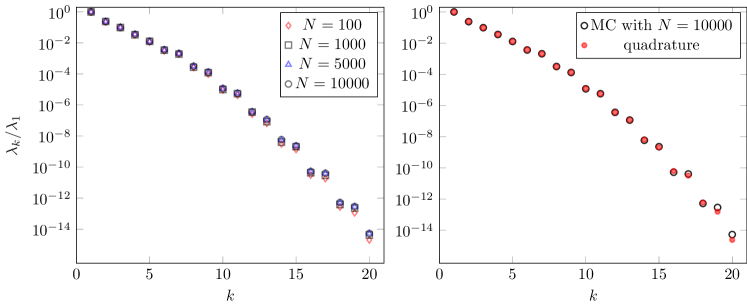
How sensitive is the discretized eigenvalue problem (25) to the number of samples $N$ used to construct the approximate covariance function $c^{N}$? We explore this issue numerically. As an initial test, Figure 4 (left) displays the first $20$ (normalized) eigenvalues of the approximate covariance operator corresponding to the oscillator example (3) as the size of Monte Carlo sample is varied. We see that even a small Monte Carlo sample (in the order of hundreds) is sufficient to capture the dominant eigenvalues of $\mathcal{C}$ for this problem. This is akin to the experiences from the computation of active subspaces [49] where the dominant eigenvalues of a covariance-like operator are considered. The impact of using approximate covariance functions on computation of spectral properties of the covariance operator is further investigated in Section 5.3.

It is also possible to approximate the covariance function via quadrature, instead of Monte Carlo, in the uncertain parameter space. Performing quadrature is generally challenging for problems with high-dimensional uncertain parameters; for such problems, full-tensor or (non-adaptive) sparse grid constructions can be computationally prohibitive due to the curse of dimensionality. However, for problems where the use of a suitable quadrature formula is feasible, this approach is preferable as it yields accurate results. In a quadrature based approach, the sample average approximations in steps 1 and 2 of Algorithm 3 are replaced by appropriate quadrature formulas. We compare the results of computing the eigenvalues of the covariance operator using a large Monte Carlo sample against a quadrature formula in Figure 4 (right).

We also mention that in numerical implementations, the discretized eigenvalue probelem (25) can be solved efficiently through Krylov iterative methods. For example we can employ the Lanczos method [50] to compute the dominant eigenpairs of the discretized covariance operator. Alternatively, one can use randomized methods such as the randomized SVD algorithm [51].

Figure 4: Eigenvalues of the discretized covariance operator for the oscillator example (3). Left: influence of the number of Monte Carlo samples $N$ on spectrum; right: comparison of the eigenvalues with the covariance function approximated via Monte Carlo sampling with $10^{4}$ samples (black circles) and through a fully tensorized Gauss-Legendre quadrature in the parameter space with $10^{3}$ nodes (solid red dots).

4.3.2 Polynomial surrogates for the KL modes (26)

Conditional expectations $\mathbb{E}\left\{{\tilde{f}_{i}({\mathchoice{\mbox{\boldmath$\displaystyle{\xi}$}}{\mbox{\boldmath$\textstyle{\xi}$}}{\mbox{\boldmath$\scriptstyle{\xi}$}}{\mbox{\boldmath$\scriptscriptstyle{\xi}$}}})|{\mathchoice{\mbox{\boldmath$\displaystyle{\xi}$}}{\mbox{\boldmath$\textstyle{\xi}$}}{\mbox{\boldmath$\scriptstyle{\xi}$}}{\mbox{\boldmath$\scriptscriptstyle{\xi}$}}}_{U}}\right\}$ can easily be computed from the PC representation for $f_{i}({\mathchoice{\mbox{\boldmath$\displaystyle{\xi}$}}{\mbox{\boldmath$\textstyle{\xi}$}}{\mbox{\boldmath$\scriptstyle{\xi}$}}{\mbox{\boldmath$\scriptscriptstyle{\xi}$}}})$

$$f_{i}({\mathchoice{\mbox{\boldmath$\displaystyle{\xi}$}}{\mbox{\boldmath$\textstyle{\xi}$}}{\mbox{\boldmath$\scriptstyle{\xi}$}}{\mbox{\boldmath$\scriptscriptstyle{\xi}$}}})\approx\tilde{f}_{i}({\mathchoice{\mbox{\boldmath$\displaystyle{\xi}$}}{\mbox{\boldmath$\textstyle{\xi}$}}{\mbox{\boldmath$\scriptstyle{\xi}$}}{\mbox{\boldmath$\scriptscriptstyle{\xi}$}}})=\sum_{k=0}^{N_{\text{PC}}}c_{k}^{i}\Psi_{k}({\mathchoice{\mbox{\boldmath$\displaystyle{\xi}$}}{\mbox{\boldmath$\textstyle{\xi}$}}{\mbox{\boldmath$\scriptstyle{\xi}$}}{\mbox{\boldmath$\scriptscriptstyle{\xi}$}}}),$$

using the tensor product construction of the PC basis, see e.g., [14]. This enables efficient computation of the generalized Sobol’ indices. For example, $\tilde{\mathfrak{{S}}}^{U}(f;T)$ with $U=\{j\}$, $j\in\{1,\ldots,{N_{\text{p}}}\}$ can be approximated as follows:

$$\mathfrak{{S}}^{j}(f;T)\approx\tilde{\mathfrak{{S}}}^{j}(f;T)=\frac{\sum_{i=1}^{N_{\text{kl}}}\sum_{k\in\mathcal{I}_{j}}\|\Psi_{k}\|^{2}(c_{k}^{i})^{2}}{\sum_{i=1}^{N_{\text{kl}}}\lambda_{i}},\quad j\in\{1,\ldots,{N_{\text{p}}}\}.$$

where $\mathcal{I}_{j}$ is an index set that picks all the terms in the PC expansion that include only $\xi_{i}$. The computation of the PC expansion coefficients for $f_{i}$ themselves can be done through a CS-based approach or NISP as outlined earlier. Note also that the generalized total Sobol’ indices can be approximated through $\tilde{\mathfrak{{S}}}^{j}_{\text{tot}}(f;T)=1-\tilde{\mathfrak{{S}}}^{U_{\sim j}}(f;T)$ with $U_{\sim j}=\{1,\ldots,{N_{\text{PC}}}\}\setminus\{j\}$.

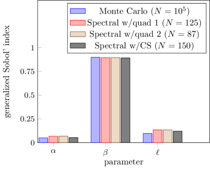
In Figure 5, we compare the performance of several options within Algorithm 3. We present results using a quadrature based approach, where we approximate the covariance function via quadrature, and compute PC representations for $f_{i}$ via NISP; specifically, we consider a full-tensor quadrature formula and a Smolyak sparse quadrature formula (see the Figure caption for more details). We also use Algorithm 3 with a small Monte Carlo sample in the uncertain parameter space, where we compute the covariance function via sample averaging, and compute the PC representations of $f_{i}$ using the CS-based approach. Moreover, we report the generalized sensitivity indices computed using direct Monte Carlo sampling with $10^{5}$ samples. Results from all approaches agree remarkably well.

Figure 5: Generalized Sobol’ indices computed via Algorithm 3 for the mechanical oscillator example (3); spectral w/quad 1: full tensor Gauss-Legendre quadrature with five nodes in each dimension, spectral w/quad 2: Smolyak sparse grid based on delayed Kronrod–Patterson rule [52, 42] and spectral CS: Monte Carlo sample of size $150$. In each case, a fourth order PC expansion for $f_{i}$, $i=1,\ldots,{N_{\text{kl}}}$, is computed (${N_{\text{kl}}}=8$).

It is important to note that Algorithm 3 utilizes the surrogate models $\tilde{f}_{i}$ to approximate the conditional expectations in the numerator of (24), as a means of approximating the generalized Sobol’ indices. This is not the same as computing the exact generalized Sobol’ indices of the approximate KL expansion, $\tilde{f}(t,{\mathchoice{\mbox{\boldmath$\displaystyle{\xi}$}}{\mbox{\boldmath$\textstyle{\xi}$}}{\mbox{\boldmath$\scriptstyle{\xi}$}}{\mbox{\boldmath$\scriptscriptstyle{\xi}$}}})=\tilde{f}_{0}(t)+\sum_{i=1}^{N_{\text{kl}}}\tilde{f}_{i}({\mathchoice{\mbox{\boldmath$\displaystyle{\xi}$}}{\mbox{\boldmath$\textstyle{\xi}$}}{\mbox{\boldmath$\scriptstyle{\xi}$}}{\mbox{\boldmath$\scriptscriptstyle{\xi}$}}})e_{i}(t)$. Another alternative approach for computing the generalized Sobol’ indices is provided by sampling the approximate truncated KL expansion of $f$, as explained below.

4.3.3 The approximate KL expansion as a global surrogate model

The computations performed in Algorithm 3 lead to an approximate KL representation of $f$,

$$f(t_{m},{\mathchoice{\mbox{\boldmath$\displaystyle{\xi}$}}{\mbox{\boldmath$\textstyle{\xi}$}}{\mbox{\boldmath$\scriptstyle{\xi}$}}{\mbox{\boldmath$\scriptscriptstyle{\xi}$}}})\approx\tilde{f}(t_{m},{\mathchoice{\mbox{\boldmath$\displaystyle{\xi}$}}{\mbox{\boldmath$\textstyle{\xi}$}}{\mbox{\boldmath$\scriptstyle{\xi}$}}{\mbox{\boldmath$\scriptscriptstyle{\xi}$}}}):=\tilde{f}_{0}(t_{m})+\sum_{i=1}^{N_{\text{kl}}}\tilde{f}_{i}({\mathchoice{\mbox{\boldmath$\displaystyle{\xi}$}}{\mbox{\boldmath$\textstyle{\xi}$}}{\mbox{\boldmath$\scriptstyle{\xi}$}}{\mbox{\boldmath$\scriptscriptstyle{\xi}$}}})e_{i}^{m},\quad m\in\{1,\ldots,{N_{\text{quad}}}\},$$ (28)

where $e_{i}^{m}$ is as in Algorithm 3, and $\tilde{f}_{0}(t_{m})$ is the sample mean, at $t=t_{m}$, computed in Algorithm 3. This provides a cheap-to-evaluate surrogate model, which can be used for an alternative approach of approximating generalized Sobol’ indices via sampling $\tilde{f}(t_{m},{\mathchoice{\mbox{\boldmath$\displaystyle{\xi}$}}{\mbox{\boldmath$\textstyle{\xi}$}}{\mbox{\boldmath$\scriptstyle{\xi}$}}{\mbox{\boldmath$\scriptscriptstyle{\xi}$}}})$. The utility of this surrogate model, however, extends beyond sensitivity analysis: $\tilde{f}(t,{\mathchoice{\mbox{\boldmath$\displaystyle{\xi}$}}{\mbox{\boldmath$\textstyle{\xi}$}}{\mbox{\boldmath$\scriptstyle{\xi}$}}{\mbox{\boldmath$\scriptscriptstyle{\xi}$}}})$ can be used to accelerate various uncertainty quantification tasks, where repeated evaluations of $f(t,{\mathchoice{\mbox{\boldmath$\displaystyle{\xi}$}}{\mbox{\boldmath$\textstyle{\xi}$}}{\mbox{\boldmath$\scriptstyle{\xi}$}}{\mbox{\boldmath$\scriptscriptstyle{\xi}$}}})$ are required. We point out that a related approach was implemented in [53] for representation of spatially distributed processes.

5 Probabilistic modeling and sensitivity analysis for a cholera model

We illustrate attributes of the generalized sensitivity indices in the context of a cholera model proposed in [54].

5.1 Model description

A population of $N_{\text{pop}}$ subjects is split, at time $t$, into $S(t)$ susceptible individuals, $I(t)$ infectious individuals, and $R(t)$ recovered individuals; the model assumes the total population $N_{\text{pop}}$ to stay constant while $S$, $I$ and $R$ vary during an epidemic with $N_{\text{pop}}=S(t)+I(t)+R(t)$. Also considered are concentrations $B_{H}(t)$ and $B_{L}(t)$ of highly- and lowly-infectious cholera bacteria, Vibrio cholerae. The units for these five state variables are compiled in Table 1. We illustrate the associated compartment model in Figure 6.

Figure 6: Compartmental cholera model from [54].

State	Symbol	Units
Susceptible Individuals	$S$	# individuals
Infected Individuals	$I$	# individuals
Recovered Individuals	$R$	# individuals
Concentration of highly-infectious	$B_{H}$	$\frac{\mbox{\rm\# bacteria}}{m\ell}$
cholera bacteria
Concentration of lowly-infectious	$B_{L}$	$\frac{\mbox{\rm\# bacteria}}{m\ell}$
cholera bacteria

Table 1: State variables and units for the cholera model.

The cholera model in [54] is based on the following assumptions. (i) The birth and death rates are identical and denoted by $b$. (ii) Susceptible individuals become infected by drinking bacteria-infested water. The rate at which this happens is proportional to $S(t)$, the concentrations $B_{H}$ and $B_{L}$ of highly and lowly-infectious bacteria, and the drinking rates $\beta_{H}$ and $\beta_{L}$ at which these bacteria are ingested. The rates also satisfy the saturation relations that when $B_{H}=\kappa_{H}$ and $B_{L}=\kappa_{L}$, where $\kappa_{H}$ and $\kappa_{L}$ denote cholera carrying capacities, the probability of ingestion resulting in disease is 0.5. Susceptibles recover at a rate $\gamma$. (iii) Infected individuals spread highly-infectious bacteria $B_{H}$ to the water at a rate $\zeta$. (iv) Highly-infectious bacteria $B_{H}$ become lowly infectious $B_{L}$ at a rate $\chi$. (v) Lowly-infectious bacteria $B_{L}$ die at a rate $\delta$.

These assumptions yield the system of ordinary differential equations (ODEs)

$$\begin{array}[]{l}{\displaystyle\frac{dS}{dt}=bN_{\text{pop}}-\beta_{L}S\frac{B_{L}}{\kappa_{L}+B_{L}}-\beta_{H}S\frac{B_{H}}{\kappa_{H}+B_{H}}-bS}\\ \vskip 6.0pt plus 2.0pt minus 2.0pt\cr{\displaystyle\frac{dI}{dt}=\beta_{L}S\frac{B_{L}}{\kappa_{L}+B_{L}}+\beta_{H}S\frac{B_{H}}{\kappa_{H}+B_{H}}-(\gamma+b)I}\\ \vskip 6.0pt plus 2.0pt minus 2.0pt\cr{\displaystyle\frac{dR}{dt}=\gamma I-bR}\\ \vskip 6.0pt plus 2.0pt minus 2.0pt\cr{\displaystyle\frac{dB_{H}}{dt}=\zeta I-\chi B_{H}}\\ \vskip 6.0pt plus 2.0pt minus 2.0pt\cr{\displaystyle\frac{dB_{L}}{dt}=\chi B_{H}-\delta B_{L}}\end{array}$$ (29)

with initial conditions $(S(0),I(0),R(0),B_{H}(0),B_{L}(0))=(S_{0},I_{0},R_{0},B_{H_{0}},B_{L_{0}})$.

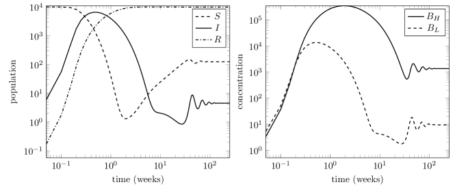
The parameter units and nominal values from [54] are compiled in Table 2. We note that $\frac{dS}{dt}+\frac{dI}{dt}+\frac{dR}{dt}=0$ so that $S(t)+I(t)+R(t)=N_{\text{pop}}$ and the population size indeed remains constant. The system dynamics are illustrated in Figure 7.

Our simulations correspond to a total population of $N_{\text{pop}}=10{,}000$ with initial states given by $S_{0}=N_{\text{pop}}-1$, $I_{0}=1$, $R_{0}=0$, and $B_{H_{0}}=B_{L_{0}}=0$. We solve the problem up to time $T=250$. The ODE system is integrated using the solver ode45 provided in Matlab ODE toolbox. We use absolute and relative tolerances of $10^{-6}$ for the ODE solver. The solution is recorded at $t_{i}=i\Delta t$, $i\in\{0,\ldots,{N_{\text{quad}}}\}$, with $\Delta t=5\times 10^{-2}$ and ${N_{\text{quad}}}=250/\Delta t$. The temporal integrals from Algorithms 2 and 3 are evaluated through the composite trapezoidal rule, where the quadrature nodes are the time steps $\{t_{i}\}_{i=0}^{N_{\text{quad}}}$.

Model Parameter	Symbol	Units	Values
Rate of drinking $B_{L}$ cholera	$\beta_{L}$	$\frac{1}{\mbox{\rm week}}$	1.5
Rate of drinking $B_{H}$ cholera	$\beta_{H}$	$\frac{1}{\mbox{\rm week}}$	7.5 ($\ast$)
$B_{L}$ cholera carrying capacity	$\kappa_{L}$	$\frac{\mbox{\rm\# bacteria}}{m\ell}$	$10^{6}$
$B_{H}$ cholera carrying capacity	$\kappa_{H}$	$\frac{\mbox{\rm\# bacteria}}{m\ell}$	$\frac{\kappa_{L}}{700}$
Human birth and death rate	$b$	$\frac{1}{\mbox{\rm week}}$	$\frac{1}{1560}$
Rate of decay from $B_{H}$ to $B_{L}$	$\chi$	$\frac{1}{\mbox{\rm week}}$	$\frac{168}{5}$
Rate at which infectious individuals	$\zeta$	$\frac{\mbox{\rm\# bacteria}}{\mbox{\rm\# individuals}\cdot m\ell\cdot\mbox{\rm week}}$	70
spread $B_{H}$ bacteria to water
Death rate of $B_{L}$ cholera	$\delta$	$\frac{1}{\mbox{\rm week}}$	$\frac{7}{30}$
Rate of recovery from cholera	$\gamma$	$\frac{1}{\mbox{\rm week}}$	$\frac{7}{5}$

Table 2: Cholera model parameters from [54].
($\ast$) The value $\beta_{H}=7.5$ is consistent with [54] where it is assumed that $\beta_{H}>\beta_{L}$; no corresponding nominal value for $\beta_{H}$ was, however, provided there.

Figure 7: Cholera model (29): time evolution of $S$, $I$, $R$, $B_{H}$, and $B_{L}$.

5.2 Statistical model for uncertain model parameters and the quantity of interest

The parameter vector ${\mathchoice{\mbox{\boldmath$\displaystyle{x}$}}{\mbox{\boldmath$\textstyle{x}$}}{\mbox{\boldmath$\scriptstyle{x}$}}{\mbox{\boldmath$\scriptscriptstyle{x}$}}}=(\beta_{L},\beta_{H},\kappa_{L},b,\chi,\zeta,\delta,\gamma)$ is considered as uncertain. The nominal values $\bar{{\mathchoice{\mbox{\boldmath$\displaystyle{x}$}}{\mbox{\boldmath$\textstyle{x}$}}{\mbox{\boldmath$\scriptstyle{x}$}}{\mbox{\boldmath$\scriptscriptstyle{x}$}}}}$ for these parameters are specified in Table 2. The distribution of these uncertain parameters is taken as uniform, with $10\%$ perturbation around the respective nominal values:

$$x_{i}=\bar{x}_{i}+0.1\bar{x}_{i}\xi_{i},\quad\xi_{i}\sim\mathcal{U}(-1,1),\quad i\in\{1,\ldots,{N_{\text{p}}}\},\quad{N_{\text{p}}}=8.$$ (30)

In [54], the nominal value of $\kappa_{H}$ is taken as ${\kappa_{L}}/{700}$. Hence, we set $\kappa_{H}=x_{3}/700$, where $x_{3}$ is as in (30).

Our quantity of interest is the infected population $I$ as a function of time. Since the vector $\textstyle{x}$ of the uncertain model parameters is defined by the random vector $\textstyle{\xi}$ in (30), we can consider the infected population as a process $I(t,{\mathchoice{\mbox{\boldmath$\displaystyle{\xi}$}}{\mbox{\boldmath$\textstyle{\xi}$}}{\mbox{\boldmath$\scriptstyle{\xi}$}}{\mbox{\boldmath$\scriptscriptstyle{\xi}$}}})$.

5.3 Global sensitivity analysis

The traditional total Sobol’ indices, computed pointwise in time, are displayed in Figure 8 (left). These indices, which show great variation over time, are difficult to interpret. This is mainly due to fact that the variance of the quantity of interest, infected population, itself varies significantly over time; see Figure 9.

Figure 8: Sensitivity analysis of the cholera model (29). Left: pointwise in time total sobol indices; right: generalized total indices over successively larger time-intervals.

Figure 9: Pointwise variance over time.

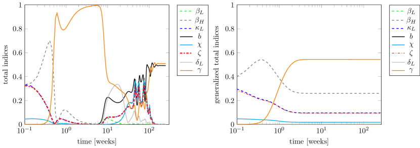
By contrast, the generalized total Sobol’ indices offer a more robust and meaningful picture; see Figure 8 (right), where generalized total indices are computed over successively larger time intervals and Figure 10 that reports the generalized Sobol’ indices corresponding to the entire simulation time interval. Note, for example, the behavior of the variable $b$: based on pointwise-in-time Sobol’ indices in Figure 8 (left), one might make the conclusion that $b$ is an important variable. However, with Figure 9 in mind, we note that $b$ becomes a major contributor to output variance around the end of the simulation time, when the model variance is at most $\mathcal{O}(1)$. In contrast, contribution of $b$ to model variance is negeligible earlier in simulation time when the model variance is $\mathcal{O}(10^{5})$. The generalized total Sobol’ indices, which are aware of the history of the process, incorporate this and accordingly rank $b$ is an unimportant variable.

Figure 10: Generalized total Sobol’ indices for the cholera model (29) with $T=250$, computed six different ways.

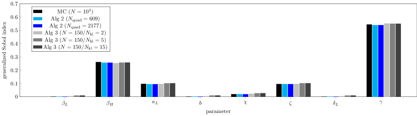
While the generalized indices are computed six different ways, as we now detail, a strong consistency can be observed in the result. When computing the generalized Sobol’ indices via Algorithm 2, we use a third-order PC expansion of $I(t,{\mathchoice{\mbox{\boldmath$\displaystyle{\xi}$}}{\mbox{\boldmath$\textstyle{\xi}$}}{\mbox{\boldmath$\scriptstyle{\xi}$}}{\mbox{\boldmath$\scriptscriptstyle{\xi}$}}})$, for each $t$ in the time grid. The PC coefficients are computed via NISP with sparse quadrature of varying resolutions. The results in Figure 10 indicate that with approximately six hundred model evaluations, it is possible to construct a PC surrogate model that is suitable for accurate estimation of the generalized Sobol’ indices.

For Algorithm 3, we use Monte Carlo sampling to approximate the covariance function and rely on the CS-based approach from Section 4.1 to approximate the fourth-order PC coefficients of the KL modes $f_{i}$ of the random process. The approach only requires a small number of model evaluations to accurately estimate the Sobol’ indices for this problem.

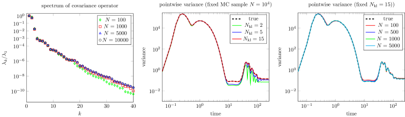
A key component of Algorithm 3 is the spectral decomposition of the covariance operator of the process. Figure 11 (left) displays the normalized eigenvalues of the covariance operator as the Monte Carlo sample size increases. We note both a rapid spectral decay and the fact that a small number of Monte Carlo samples is sufficient to accurately estimate the dominant eigenvalues. As shown in Figure 11 (middle), the evolution of the pointwise covariance, computed using a truncated KL expansion, can be quantified accurately with a small number of KL modes. Indeed, ${N_{\text{kl}}}=15$ modes is sufficient; in fact, only two KL modes can be used in the interval $[0,1]$; i.e., during the transient regime.

The computation in Figure 11 (middle) uses a fixed Monte Carlo sample of size $N=10^{4}$. From the results in Figure 11 (left), we know that a much smaller Monte Carlo sample is sufficient for approximating the dominant eigenvalues. However, the computation of the pointwise variance depends also on approximation of the eigenvectors of the covariance operator. Instead of performing convergence studies for the dominant eigenvectors, we consider the following question: how does the approximation of the pointwise variance change for ${N_{\text{kl}}}=15$ if we use smaller Monte Carlo samples? This is investigated in Figure 11 (right) which confirms that a small Monte Carlo sample enables accurate estimation of the pointwise variance, as computed by an approximate truncated KL expansion.

Figure 11: Spectral properties and variance analysis of the cholera model (29). Left: spectrum of the sampled covariance operator from Section 4.2; middle: pointwise variance of the truncated process $f^{({{N_{\text{kl}}}})}(t,{\mathchoice{\mbox{\boldmath$\displaystyle{\xi}$}}{\mbox{\boldmath$\textstyle{\xi}$}}{\mbox{\boldmath$\scriptstyle{\xi}$}}{\mbox{\boldmath$\scriptscriptstyle{\xi}$}}})$ with $N=10^{4}$ samples to approximate the covariance function. Right: pointwise variance of the truncated process $f^{({{N_{\text{kl}}}})}(t,{\mathchoice{\mbox{\boldmath$\displaystyle{\xi}$}}{\mbox{\boldmath$\textstyle{\xi}$}}{\mbox{\boldmath$\scriptstyle{\xi}$}}{\mbox{\boldmath$\scriptscriptstyle{\xi}$}}})$ with ${N_{\text{kl}}}=15$ and with varying Monte Carlo sample sizes used to approximate the covariance function.

5.4 Generalized Sobol’ indices for parameter dimension reduction

Based on generalized Sobol’ indices on the interval $[0,250]$, the important variables are $\beta_{H}$, $\kappa_{L}$, $\zeta$, and $\gamma$. This suggests that we can reduce the parameter dimension by fixing the remaining variables at their nominal values. We provide next a numerical study of the approximation errors which result from fixing inessential variables. To illustrate the potential pitfalls of fixing parameters based on pointwise in time classical Sobol’ indices, we also consider fixing parameters according to the classical Sobol’ indices at $t=250$, which indicate $b$ and $\gamma$ as the important parameters.

When fixing inessential variables, we consider the reduced model

$$\tilde{I}_{u}(t,{\mathchoice{\mbox{\boldmath$\displaystyle{\xi}$}}{\mbox{\boldmath$\textstyle{\xi}$}}{\mbox{\boldmath$\scriptstyle{\xi}$}}{\mbox{\boldmath$\scriptscriptstyle{\xi}$}}})=I(t,\tilde{\mathchoice{\mbox{\boldmath$\displaystyle{\xi}$}}{\mbox{\boldmath$\textstyle{\xi}$}}{\mbox{\boldmath$\scriptstyle{\xi}$}}{\mbox{\boldmath$\scriptscriptstyle{\xi}$}}}),\quad\text{with }\tilde{\mathchoice{\mbox{\boldmath$\displaystyle{\xi}$}}{\mbox{\boldmath$\textstyle{\xi}$}}{\mbox{\boldmath$\scriptstyle{\xi}$}}{\mbox{\boldmath$\scriptscriptstyle{\xi}$}}}=({\mathchoice{\mbox{\boldmath$\displaystyle{\xi}$}}{\mbox{\boldmath$\textstyle{\xi}$}}{\mbox{\boldmath$\scriptstyle{\xi}$}}{\mbox{\boldmath$\scriptscriptstyle{\xi}$}}}_{U},{\mathchoice{\mbox{\boldmath$\displaystyle{\xi}$}}{\mbox{\boldmath$\textstyle{\xi}$}}{\mbox{\boldmath$\scriptstyle{\xi}$}}{\mbox{\boldmath$\scriptscriptstyle{\xi}$}}}_{U^{\complement}}^{\text{nom}}),\quad U\subseteq X=\{1,\ldots,{N_{\text{p}}}\}.$$

To provide a thorough study, we examine the impact of fixing parameters on pointwise variance and the distribution of the process.

Figure 12: Effect of fixing inessential variables for the cholera model (29). Left: effect on the variance; middle: effect on the quantity of interest when using generalized indices; right: effect on the quantity of interest when using pointwise indices at the final time.

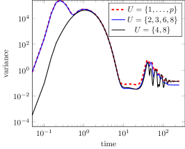
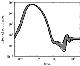
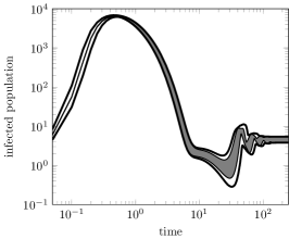
Figure 12 (left) illustrates the impact of fixing inessential variables on the variance of the process over time. The effect on the distribution of the process itself is studied in Figures 12 (middle) and (right), where important variables are chosen based on generalized Sobol’ indices and based on pointwise Sobol’ indices at the final time, respectively. The thick black lines indicate the $2$nd and $98$th percentiles obtained by sampling $I(t,{\mathchoice{\mbox{\boldmath$\displaystyle{\xi}$}}{\mbox{\boldmath$\textstyle{\xi}$}}{\mbox{\boldmath$\scriptstyle{\xi}$}}{\mbox{\boldmath$\scriptscriptstyle{\xi}$}}})$ (with no variables fixed) $10^{4}$ times. The shaded regions enclose the respective percentiles for $\tilde{I}(t,{\mathchoice{\mbox{\boldmath$\displaystyle{\xi}$}}{\mbox{\boldmath$\textstyle{\xi}$}}{\mbox{\boldmath$\scriptstyle{\xi}$}}{\mbox{\boldmath$\scriptscriptstyle{\xi}$}}})$, which is also obtained by sampling the reduced models $10^{4}$ times.

We note that fixing variables according to generalized indices results in a reduced model that captures the distribution of $I$ over the simulation time window well. On the other hand, and as expected, fixing variables according to pointwise Sobol’ indices at the final time is effective at capturing the distribution of $I$ only as the system approaches equilibrium. In Figure 13, we study the impact of fixing variables on the probability density function (PDF) of the infected population over time. These PDFs were generated by sampling the reduced models $10^{4}$ times.

Figure 13: Effect of fixing inessential variables, chosen according to generalized indices (indicated as $\tilde{I}_{1}$) and Sobol’ indices at final time (indicated as $\tilde{I}_{2}$) on distribution of the infected population for the cholera model (29).

6 Conclusions

The global sensitivity analysis of time-dependent processes such as (1) requires history-aware approaches. Not surprisingly, identifying inessential parameters based on a pointwise in time analysis, such as the one corresponding to the standard Sobol’ indices, is only valid close to the time at which the analysis is performed. For applications where the evolution of the process under study is of interest, sensitivity analysis must be performed globally in time.

We show how to efficiently compute generalized Sobol’ indices. The various tests of the impact of fixing inessential parameters provide a consistent picture: using generalized total Sobol’ indices, we can reliably select the variables with dominant impact on variability of the quantity of interest. Further formalization of these results in the form of, for instance, theoretical error analysis is to our knowledge not available but is desirable. Likewise, the global sensitivity analysis of time-dependent processes with correlated parameters is beyond this work and deserves further investigation.

Appendix A Definition of the index set $\mathcal{K}_{i}$

Here we briefly explain the definition of the index set $\mathcal{K}_{i}$ in (21). We use a multivariate PC basis that is obtained through partial tensorization of appropriate univariate bases. More precisely, if we denote by $\{\psi_{j}(\xi_{i})\}_{j=1}^{\infty}$ the univariate orthogonal polynomial basis corresponding to $\xi_{i}$, we form the multivariate PC basis $\{\Psi_{k}\}_{k=0}^{\infty}$ as follows:

$$\Psi_{k}({\mathchoice{\mbox{\boldmath$\displaystyle{\xi}$}}{\mbox{\boldmath$\textstyle{\xi}$}}{\mbox{\boldmath$\scriptstyle{\xi}$}}{\mbox{\boldmath$\scriptscriptstyle{\xi}$}}})=\prod_{i=1}^{{N_{\text{p}}}}\psi_{\alpha_{i}^{k}}(\xi_{i}),\qquad{\mathchoice{\mbox{\boldmath$\displaystyle{\xi}$}}{\mbox{\boldmath$\textstyle{\xi}$}}{\mbox{\boldmath$\scriptstyle{\xi}$}}{\mbox{\boldmath$\scriptscriptstyle{\xi}$}}}\in\Omega,\,k=0,1,2,\ldots,$$ (31)

where ${\mathchoice{\mbox{\boldmath$\displaystyle{\alpha}$}}{\mbox{\boldmath$\textstyle{\alpha}$}}{\mbox{\boldmath$\scriptstyle{\alpha}$}}{\mbox{\boldmath$\scriptscriptstyle{\alpha}$}}}^{k}=\left(\alpha_{1}^{k},\alpha_{2}^{k},\cdots,\alpha_{N_{\text{p}}}^{k}\right)$, with $\alpha_{k}^{i}\geq 0$ for $i=1,\ldots,{N_{\text{p}}}$, is a multi-index, and $\alpha_{i}^{k}$ indicates the order of the univariate polynomials in $\xi_{i}$. In the present context, where $\xi_{i}$ is uniformly distributed, $\psi_{\alpha_{i}^{k}}$ is the Legendre polynomial of order $\alpha_{i}^{k}$. An indexing scheme for the multi-indices $\{{\mathchoice{\mbox{\boldmath$\displaystyle{\alpha}$}}{\mbox{\boldmath$\textstyle{\alpha}$}}{\mbox{\boldmath$\scriptstyle{\alpha}$}}{\mbox{\boldmath$\scriptscriptstyle{\alpha}$}}}^{k}\}_{k=0}^{{N_{\text{p}}}}$, which is convenient for computer implementations, can be found for instance in [10, Appendix C.]. The multivariate orthogonal polynomial basis functions defined in (31) are used in the PC expansion of $f(t,{\mathchoice{\mbox{\boldmath$\displaystyle{\xi}$}}{\mbox{\boldmath$\textstyle{\xi}$}}{\mbox{\boldmath$\scriptstyle{\xi}$}}{\mbox{\boldmath$\scriptscriptstyle{\xi}$}}})$ in (17).

The index set $\mathcal{K}_{i}$ in (21), which picks all the terms in the PC expansion that include $\xi_{i}$, is given by $\mathcal{K}_{i}=\big{\{}k\in\{1,\ldots,{N_{\text{PC}}}\}:\alpha_{k}^{i}>0\big{\}}$.

Appendix B Proof of Theorem 4.1

First we establish some technical lemmas.

Lemma 1.

Let $f$ be a centered process satisfying the assumptions of Section 2 and let $\mathcal{C}$ be its covariance operator with eigenpairs $\{(\lambda_{i},e_{i})\}_{i=1}^{\infty}$. The following hold:

1. $\mathbb{E}\left\{{f^{(n)}}\right\}=0$,

2. $\mathbb{V}\left\{{f^{(n)}(t,{\mathchoice{\mbox{\boldmath$\displaystyle{\xi}$}}{\mbox{\boldmath$\textstyle{\xi}$}}{\mbox{\boldmath$\scriptstyle{\xi}$}}{\mbox{\boldmath$\scriptscriptstyle{\xi}$}}})}\right\}=\sum_{i=1}^{n}\lambda_{i}e_{i}(t)^{2}$,

3. We have

   $$\lim_{n\to\infty}\int_{0}^{T}\mathbb{V}\left\{{f^{(n)}(t,{\mathchoice{\mbox{\boldmath$\displaystyle{\xi}$}}{\mbox{\boldmath$\textstyle{\xi}$}}{\mbox{\boldmath$\scriptstyle{\xi}$}}{\mbox{\boldmath$\scriptscriptstyle{\xi}$}}})}\right\}\,dt=\int_{0}^{T}\mathbb{V}\left\{{f(t,{\mathchoice{\mbox{\boldmath$\displaystyle{\xi}$}}{\mbox{\boldmath$\textstyle{\xi}$}}{\mbox{\boldmath$\scriptstyle{\xi}$}}{\mbox{\boldmath$\scriptscriptstyle{\xi}$}}})}\right\}\,dt.$$

Proof.

The first statement is clear. The second statement is seen as follows:

$$\mathbb{V}\left\{{f^{(n)}(t,{\mathchoice{\mbox{\boldmath$\displaystyle{\xi}$}}{\mbox{\boldmath$\textstyle{\xi}$}}{\mbox{\boldmath$\scriptstyle{\xi}$}}{\mbox{\boldmath$\scriptscriptstyle{\xi}$}}})}\right\}=\mathbb{E}\left\{{f^{(n)}(t,{\mathchoice{\mbox{\boldmath$\displaystyle{\xi}$}}{\mbox{\boldmath$\textstyle{\xi}$}}{\mbox{\boldmath$\scriptstyle{\xi}$}}{\mbox{\boldmath$\scriptscriptstyle{\xi}$}}})^{2}}\right\}=\mathbb{E}\left\{{\left(\sum_{i=1}^{n}f_{i}({\mathchoice{\mbox{\boldmath$\displaystyle{\xi}$}}{\mbox{\boldmath$\textstyle{\xi}$}}{\mbox{\boldmath$\scriptstyle{\xi}$}}{\mbox{\boldmath$\scriptscriptstyle{\xi}$}}})e_{i}(t)\right)\left(\sum_{j=1}^{n}f_{j}({\mathchoice{\mbox{\boldmath$\displaystyle{\xi}$}}{\mbox{\boldmath$\textstyle{\xi}$}}{\mbox{\boldmath$\scriptstyle{\xi}$}}{\mbox{\boldmath$\scriptscriptstyle{\xi}$}}})e_{j}(t)\right)}\right\}\\ =\sum_{i,j}\mathbb{E}\left\{{f_{i}f_{j}}\right\}e_{i}(t)e_{j}(t)=\sum_{i=1}^{n}\lambda_{i}e_{i}(t)^{2}.$$ (32)

Finally, the third statement is derived as follows:

$$\lim_{n\to\infty}\int_{0}^{T}\mathbb{V}\left\{{f^{(n)}(t,{\mathchoice{\mbox{\boldmath$\displaystyle{\xi}$}}{\mbox{\boldmath$\textstyle{\xi}$}}{\mbox{\boldmath$\scriptstyle{\xi}$}}{\mbox{\boldmath$\scriptscriptstyle{\xi}$}}})}\right\}=\lim_{n\to\infty}\int_{0}^{T}\sum_{i=1}^{n}\lambda_{i}e_{i}(t)^{2}\,dt=\lim_{n\to\infty}\sum_{i=1}^{n}\lambda_{i}\,dt\\ =\mathrm{Tr}(\mathcal{C})=\int_{0}^{T}c(t,t)\,dt=\int_{0}^{T}\mathbb{V}\left\{{f(t,{\mathchoice{\mbox{\boldmath$\displaystyle{\xi}$}}{\mbox{\boldmath$\textstyle{\xi}$}}{\mbox{\boldmath$\scriptstyle{\xi}$}}{\mbox{\boldmath$\scriptscriptstyle{\xi}$}}})}\right\}\,dt,$$

where the penultimate equality follows from Mercer’s Theorem. ∎

Lemma 2.

Let $f$ be a centered process satisfying the assumptions of Section 2. Then, for $U\subset\{1,\ldots,{N_{\text{p}}}\}$,

$$\lim_{n\to\infty}\mathbb{V}\left\{{\mathbb{E}\left\{{f^{(n)}(t,{\mathchoice{\mbox{\boldmath$\displaystyle{\xi}$}}{\mbox{\boldmath$\textstyle{\xi}$}}{\mbox{\boldmath$\scriptstyle{\xi}$}}{\mbox{\boldmath$\scriptscriptstyle{\xi}$}}})|{\mathchoice{\mbox{\boldmath$\displaystyle{\xi}$}}{\mbox{\boldmath$\textstyle{\xi}$}}{\mbox{\boldmath$\scriptstyle{\xi}$}}{\mbox{\boldmath$\scriptscriptstyle{\xi}$}}}_{U}}\right\}}\right\}=\mathbb{V}\left\{{\mathbb{E}\left\{{f(t,{\mathchoice{\mbox{\boldmath$\displaystyle{\xi}$}}{\mbox{\boldmath$\textstyle{\xi}$}}{\mbox{\boldmath$\scriptstyle{\xi}$}}{\mbox{\boldmath$\scriptscriptstyle{\xi}$}}})|{\mathchoice{\mbox{\boldmath$\displaystyle{\xi}$}}{\mbox{\boldmath$\textstyle{\xi}$}}{\mbox{\boldmath$\scriptstyle{\xi}$}}{\mbox{\boldmath$\scriptscriptstyle{\xi}$}}}_{U}}\right\}}\right\}.$$

Proof.

Let $t\in[0,T]$ be fixed but arbitrary. Since $f^{(n)}(t,{\mathchoice{\mbox{\boldmath$\displaystyle{\xi}$}}{\mbox{\boldmath$\textstyle{\xi}$}}{\mbox{\boldmath$\scriptstyle{\xi}$}}{\mbox{\boldmath$\scriptscriptstyle{\xi}$}}})\to f(t,{\mathchoice{\mbox{\boldmath$\displaystyle{\xi}$}}{\mbox{\boldmath$\textstyle{\xi}$}}{\mbox{\boldmath$\scriptstyle{\xi}$}}{\mbox{\boldmath$\scriptscriptstyle{\xi}$}}})$ in $L^{2}(\Omega)$, by properties of conditional expectation $\mathbb{E}\left\{{f^{(n)}(t,{\mathchoice{\mbox{\boldmath$\displaystyle{\xi}$}}{\mbox{\boldmath$\textstyle{\xi}$}}{\mbox{\boldmath$\scriptstyle{\xi}$}}{\mbox{\boldmath$\scriptscriptstyle{\xi}$}}})|{\mathchoice{\mbox{\boldmath$\displaystyle{\xi}$}}{\mbox{\boldmath$\textstyle{\xi}$}}{\mbox{\boldmath$\scriptstyle{\xi}$}}{\mbox{\boldmath$\scriptscriptstyle{\xi}$}}}_{U}}\right\}\to\mathbb{E}\left\{{f(t,{\mathchoice{\mbox{\boldmath$\displaystyle{\xi}$}}{\mbox{\boldmath$\textstyle{\xi}$}}{\mbox{\boldmath$\scriptstyle{\xi}$}}{\mbox{\boldmath$\scriptscriptstyle{\xi}$}}})|{\mathchoice{\mbox{\boldmath$\displaystyle{\xi}$}}{\mbox{\boldmath$\textstyle{\xi}$}}{\mbox{\boldmath$\scriptstyle{\xi}$}}{\mbox{\boldmath$\scriptscriptstyle{\xi}$}}}_{U}}\right\}$ in $L^{2}(\Omega)$. Next, noting that, $\mathbb{E}\left\{{\mathbb{E}\left\{{f^{(n)}(t,{\mathchoice{\mbox{\boldmath$\displaystyle{\xi}$}}{\mbox{\boldmath$\textstyle{\xi}$}}{\mbox{\boldmath$\scriptstyle{\xi}$}}{\mbox{\boldmath$\scriptscriptstyle{\xi}$}}})|{\mathchoice{\mbox{\boldmath$\displaystyle{\xi}$}}{\mbox{\boldmath$\textstyle{\xi}$}}{\mbox{\boldmath$\scriptstyle{\xi}$}}{\mbox{\boldmath$\scriptscriptstyle{\xi}$}}}_{U}}\right\}}\right\}=0$, we obtain

$$\left|\mathbb{V}\left\{{\mathbb{E}\left\{{f^{(n)}(t,{\mathchoice{\mbox{\boldmath$\displaystyle{\xi}$}}{\mbox{\boldmath$\textstyle{\xi}$}}{\mbox{\boldmath$\scriptstyle{\xi}$}}{\mbox{\boldmath$\scriptscriptstyle{\xi}$}}})|{\mathchoice{\mbox{\boldmath$\displaystyle{\xi}$}}{\mbox{\boldmath$\textstyle{\xi}$}}{\mbox{\boldmath$\scriptstyle{\xi}$}}{\mbox{\boldmath$\scriptscriptstyle{\xi}$}}}_{U}}\right\}}\right\}-\mathbb{V}\left\{{\mathbb{E}\left\{{f(t,{\mathchoice{\mbox{\boldmath$\displaystyle{\xi}$}}{\mbox{\boldmath$\textstyle{\xi}$}}{\mbox{\boldmath$\scriptstyle{\xi}$}}{\mbox{\boldmath$\scriptscriptstyle{\xi}$}}})|{\mathchoice{\mbox{\boldmath$\displaystyle{\xi}$}}{\mbox{\boldmath$\textstyle{\xi}$}}{\mbox{\boldmath$\scriptstyle{\xi}$}}{\mbox{\boldmath$\scriptscriptstyle{\xi}$}}}_{U}}\right\}}\right\}\right|=\left|\|{\mathbb{E}\left\{{f^{(n)}(t,{\mathchoice{\mbox{\boldmath$\displaystyle{\xi}$}}{\mbox{\boldmath$\textstyle{\xi}$}}{\mbox{\boldmath$\scriptstyle{\xi}$}}{\mbox{\boldmath$\scriptscriptstyle{\xi}$}}})|{\mathchoice{\mbox{\boldmath$\displaystyle{\xi}$}}{\mbox{\boldmath$\textstyle{\xi}$}}{\mbox{\boldmath$\scriptstyle{\xi}$}}{\mbox{\boldmath$\scriptscriptstyle{\xi}$}}}_{U}}\right\}}\|_{L^{2}(\Omega)}^{2}-\|{\mathbb{E}\left\{{f(t,{\mathchoice{\mbox{\boldmath$\displaystyle{\xi}$}}{\mbox{\boldmath$\textstyle{\xi}$}}{\mbox{\boldmath$\scriptstyle{\xi}$}}{\mbox{\boldmath$\scriptscriptstyle{\xi}$}}})|{\mathchoice{\mbox{\boldmath$\displaystyle{\xi}$}}{\mbox{\boldmath$\textstyle{\xi}$}}{\mbox{\boldmath$\scriptstyle{\xi}$}}{\mbox{\boldmath$\scriptscriptstyle{\xi}$}}}_{U}}\right\}}\|_{L^{2}(\Omega)}^{2}\right|\to 0,$$

as $n\to\infty$. ∎

Proof of Theorem 4.1. We begin by considering $\lim_{n\to\infty}\int_{0}^{T}\mathbb{V}\left\{{\mathbb{E}\left\{{f^{(n)}(t,{\mathchoice{\mbox{\boldmath$\displaystyle{\xi}$}}{\mbox{\boldmath$\textstyle{\xi}$}}{\mbox{\boldmath$\scriptstyle{\xi}$}}{\mbox{\boldmath$\scriptscriptstyle{\xi}$}}})|{\mathchoice{\mbox{\boldmath$\displaystyle{\xi}$}}{\mbox{\boldmath$\textstyle{\xi}$}}{\mbox{\boldmath$\scriptstyle{\xi}$}}{\mbox{\boldmath$\scriptscriptstyle{\xi}$}}}_{U}}\right\}}\right\}\,dt$. We have $\mathbb{V}\left\{{\mathbb{E}\left\{{f^{(n)}(t,{\mathchoice{\mbox{\boldmath$\displaystyle{\xi}$}}{\mbox{\boldmath$\textstyle{\xi}$}}{\mbox{\boldmath$\scriptstyle{\xi}$}}{\mbox{\boldmath$\scriptscriptstyle{\xi}$}}})|{\mathchoice{\mbox{\boldmath$\displaystyle{\xi}$}}{\mbox{\boldmath$\textstyle{\xi}$}}{\mbox{\boldmath$\scriptstyle{\xi}$}}{\mbox{\boldmath$\scriptscriptstyle{\xi}$}}}_{U}}\right\}}\right\}\leq\mathbb{V}\left\{{f^{(n)}(t,{\mathchoice{\mbox{\boldmath$\displaystyle{\xi}$}}{\mbox{\boldmath$\textstyle{\xi}$}}{\mbox{\boldmath$\scriptstyle{\xi}$}}{\mbox{\boldmath$\scriptscriptstyle{\xi}$}}})}\right\}\leq\mathbb{V}\left\{{f(t,{\mathchoice{\mbox{\boldmath$\displaystyle{\xi}$}}{\mbox{\boldmath$\textstyle{\xi}$}}{\mbox{\boldmath$\scriptstyle{\xi}$}}{\mbox{\boldmath$\scriptscriptstyle{\xi}$}}})}\right\}$, and $\mathbb{V}\left\{{f(t,{\mathchoice{\mbox{\boldmath$\displaystyle{\xi}$}}{\mbox{\boldmath$\textstyle{\xi}$}}{\mbox{\boldmath$\scriptstyle{\xi}$}}{\mbox{\boldmath$\scriptscriptstyle{\xi}$}}})}\right\}\in L^{2}(0,T)$. Therefore, by Lemma 2 and the Lebesgue Dominated Convergence Theorem,

$$\lim_{n\to\infty}\int_{0}^{T}\mathbb{V}\left\{{\mathbb{E}\left\{{f^{(n)}(t,{\mathchoice{\mbox{\boldmath$\displaystyle{\xi}$}}{\mbox{\boldmath$\textstyle{\xi}$}}{\mbox{\boldmath$\scriptstyle{\xi}$}}{\mbox{\boldmath$\scriptscriptstyle{\xi}$}}})|{\mathchoice{\mbox{\boldmath$\displaystyle{\xi}$}}{\mbox{\boldmath$\textstyle{\xi}$}}{\mbox{\boldmath$\scriptstyle{\xi}$}}{\mbox{\boldmath$\scriptscriptstyle{\xi}$}}}_{U}}\right\}}\right\}\,dt=\int_{0}^{T}\mathbb{V}\left\{{\mathbb{E}\left\{{f(t,{\mathchoice{\mbox{\boldmath$\displaystyle{\xi}$}}{\mbox{\boldmath$\textstyle{\xi}$}}{\mbox{\boldmath$\scriptstyle{\xi}$}}{\mbox{\boldmath$\scriptscriptstyle{\xi}$}}})|{\mathchoice{\mbox{\boldmath$\displaystyle{\xi}$}}{\mbox{\boldmath$\textstyle{\xi}$}}{\mbox{\boldmath$\scriptstyle{\xi}$}}{\mbox{\boldmath$\scriptscriptstyle{\xi}$}}}_{U}}\right\}}\right\}\,dt.$$

This, along with Lemma 1(3), yields

$$\lim_{n\to\infty}\frac{\int_{0}^{T}\mathbb{V}\left\{{\mathbb{E}\left\{{f^{(n)}(t,{\mathchoice{\mbox{\boldmath$\displaystyle{\xi}$}}{\mbox{\boldmath$\textstyle{\xi}$}}{\mbox{\boldmath$\scriptstyle{\xi}$}}{\mbox{\boldmath$\scriptscriptstyle{\xi}$}}})|{\mathchoice{\mbox{\boldmath$\displaystyle{\xi}$}}{\mbox{\boldmath$\textstyle{\xi}$}}{\mbox{\boldmath$\scriptstyle{\xi}$}}{\mbox{\boldmath$\scriptscriptstyle{\xi}$}}}_{U}}\right\}}\right\}\,dt}{\int_{0}^{T}\mathbb{V}\left\{{f^{(n)}(t,{\mathchoice{\mbox{\boldmath$\displaystyle{\xi}$}}{\mbox{\boldmath$\textstyle{\xi}$}}{\mbox{\boldmath$\scriptstyle{\xi}$}}{\mbox{\boldmath$\scriptscriptstyle{\xi}$}}})}\right\}\,dt}=\frac{\int_{0}^{T}\mathbb{V}\left\{{\mathbb{E}\left\{{f(t,{\mathchoice{\mbox{\boldmath$\displaystyle{\xi}$}}{\mbox{\boldmath$\textstyle{\xi}$}}{\mbox{\boldmath$\scriptstyle{\xi}$}}{\mbox{\boldmath$\scriptscriptstyle{\xi}$}}})|{\mathchoice{\mbox{\boldmath$\displaystyle{\xi}$}}{\mbox{\boldmath$\textstyle{\xi}$}}{\mbox{\boldmath$\scriptstyle{\xi}$}}{\mbox{\boldmath$\scriptscriptstyle{\xi}$}}}_{U}}\right\}}\right\}\,dt}{\int_{0}^{T}\mathbb{V}\left\{{f(t,{\mathchoice{\mbox{\boldmath$\displaystyle{\xi}$}}{\mbox{\boldmath$\textstyle{\xi}$}}{\mbox{\boldmath$\scriptstyle{\xi}$}}{\mbox{\boldmath$\scriptscriptstyle{\xi}$}}})}\right\}\,dt}=\mathfrak{{S}}^{U}(f;T).$$ (33)

Next, note that, $\mathbb{E}\left\{{f^{(n)}(t,{\mathchoice{\mbox{\boldmath$\displaystyle{\xi}$}}{\mbox{\boldmath$\textstyle{\xi}$}}{\mbox{\boldmath$\scriptstyle{\xi}$}}{\mbox{\boldmath$\scriptscriptstyle{\xi}$}}})|{\mathchoice{\mbox{\boldmath$\displaystyle{\xi}$}}{\mbox{\boldmath$\textstyle{\xi}$}}{\mbox{\boldmath$\scriptstyle{\xi}$}}{\mbox{\boldmath$\scriptscriptstyle{\xi}$}}}_{U}}\right\}=\mathbb{E}\left\{{\sum_{i=1}^{n}f_{i}({\mathchoice{\mbox{\boldmath$\displaystyle{\xi}$}}{\mbox{\boldmath$\textstyle{\xi}$}}{\mbox{\boldmath$\scriptstyle{\xi}$}}{\mbox{\boldmath$\scriptscriptstyle{\xi}$}}})e_{i}(t)|{\mathchoice{\mbox{\boldmath$\displaystyle{\xi}$}}{\mbox{\boldmath$\textstyle{\xi}$}}{\mbox{\boldmath$\scriptstyle{\xi}$}}{\mbox{\boldmath$\scriptscriptstyle{\xi}$}}}_{U}}\right\}=\sum_{i=1}^{n}\mathbb{E}\left\{{f_{i}({\mathchoice{\mbox{\boldmath$\displaystyle{\xi}$}}{\mbox{\boldmath$\textstyle{\xi}$}}{\mbox{\boldmath$\scriptstyle{\xi}$}}{\mbox{\boldmath$\scriptscriptstyle{\xi}$}}})|{\mathchoice{\mbox{\boldmath$\displaystyle{\xi}$}}{\mbox{\boldmath$\textstyle{\xi}$}}{\mbox{\boldmath$\scriptstyle{\xi}$}}{\mbox{\boldmath$\scriptscriptstyle{\xi}$}}}_{U}}\right\}e_{i}(t)$. Then, we proceed as follows:

$$\int_{0}^{T}\mathbb{V}\left\{{\mathbb{E}\left\{{f^{(n)}(t,{\mathchoice{\mbox{\boldmath$\displaystyle{\xi}$}}{\mbox{\boldmath$\textstyle{\xi}$}}{\mbox{\boldmath$\scriptstyle{\xi}$}}{\mbox{\boldmath$\scriptscriptstyle{\xi}$}}})|{\mathchoice{\mbox{\boldmath$\displaystyle{\xi}$}}{\mbox{\boldmath$\textstyle{\xi}$}}{\mbox{\boldmath$\scriptstyle{\xi}$}}{\mbox{\boldmath$\scriptscriptstyle{\xi}$}}}_{U}}\right\}}\right\}\,dt =\int_{0}^{T}\mathbb{V}\left\{{\sum_{i=1}^{n}\mathbb{E}\left\{{f_{i}({\mathchoice{\mbox{\boldmath$\displaystyle{\xi}$}}{\mbox{\boldmath$\textstyle{\xi}$}}{\mbox{\boldmath$\scriptstyle{\xi}$}}{\mbox{\boldmath$\scriptscriptstyle{\xi}$}}})|{\mathchoice{\mbox{\boldmath$\displaystyle{\xi}$}}{\mbox{\boldmath$\textstyle{\xi}$}}{\mbox{\boldmath$\scriptstyle{\xi}$}}{\mbox{\boldmath$\scriptscriptstyle{\xi}$}}}_{U}}\right\}e_{i}(t)}\right\}\,dt$$

$$=\int_{0}^{T}\mathbb{E}\left\{{\Big{(}\sum_{i=1}^{n}\mathbb{E}\left\{{f_{i}({\mathchoice{\mbox{\boldmath$\displaystyle{\xi}$}}{\mbox{\boldmath$\textstyle{\xi}$}}{\mbox{\boldmath$\scriptstyle{\xi}$}}{\mbox{\boldmath$\scriptscriptstyle{\xi}$}}})|{\mathchoice{\mbox{\boldmath$\displaystyle{\xi}$}}{\mbox{\boldmath$\textstyle{\xi}$}}{\mbox{\boldmath$\scriptstyle{\xi}$}}{\mbox{\boldmath$\scriptscriptstyle{\xi}$}}}_{U}}\right\}e_{i}(t)\Big{)}^{2}}\right\}\,dt$$

$$=\mathbb{E}\left\{{\int_{0}^{T}\Big{(}\sum_{i=1}^{n}\mathbb{E}\left\{{f_{i}({\mathchoice{\mbox{\boldmath$\displaystyle{\xi}$}}{\mbox{\boldmath$\textstyle{\xi}$}}{\mbox{\boldmath$\scriptstyle{\xi}$}}{\mbox{\boldmath$\scriptscriptstyle{\xi}$}}})|{\mathchoice{\mbox{\boldmath$\displaystyle{\xi}$}}{\mbox{\boldmath$\textstyle{\xi}$}}{\mbox{\boldmath$\scriptstyle{\xi}$}}{\mbox{\boldmath$\scriptscriptstyle{\xi}$}}}_{U}}\right\}e_{i}(t)\Big{)}^{2}\,dt}\right\}$$

$$=\mathbb{E}\left\{{\sum_{i,k=1}^{n}\mathbb{E}\left\{{f_{i}({\mathchoice{\mbox{\boldmath$\displaystyle{\xi}$}}{\mbox{\boldmath$\textstyle{\xi}$}}{\mbox{\boldmath$\scriptstyle{\xi}$}}{\mbox{\boldmath$\scriptscriptstyle{\xi}$}}})|{\mathchoice{\mbox{\boldmath$\displaystyle{\xi}$}}{\mbox{\boldmath$\textstyle{\xi}$}}{\mbox{\boldmath$\scriptstyle{\xi}$}}{\mbox{\boldmath$\scriptscriptstyle{\xi}$}}}_{U}}\right\}\mathbb{E}\left\{{f_{k}({\mathchoice{\mbox{\boldmath$\displaystyle{\xi}$}}{\mbox{\boldmath$\textstyle{\xi}$}}{\mbox{\boldmath$\scriptstyle{\xi}$}}{\mbox{\boldmath$\scriptscriptstyle{\xi}$}}})|{\mathchoice{\mbox{\boldmath$\displaystyle{\xi}$}}{\mbox{\boldmath$\textstyle{\xi}$}}{\mbox{\boldmath$\scriptstyle{\xi}$}}{\mbox{\boldmath$\scriptscriptstyle{\xi}$}}}_{U}}\right\}\int_{0}^{T}e_{i}(t)e_{k}(t)\,dt}\right\}$$

$$=\mathbb{E}\left\{{\sum_{i=1}^{n}\mathbb{E}\left\{{f_{i}({\mathchoice{\mbox{\boldmath$\displaystyle{\xi}$}}{\mbox{\boldmath$\textstyle{\xi}$}}{\mbox{\boldmath$\scriptstyle{\xi}$}}{\mbox{\boldmath$\scriptscriptstyle{\xi}$}}})|{\mathchoice{\mbox{\boldmath$\displaystyle{\xi}$}}{\mbox{\boldmath$\textstyle{\xi}$}}{\mbox{\boldmath$\scriptstyle{\xi}$}}{\mbox{\boldmath$\scriptscriptstyle{\xi}$}}}_{U}}\right\}^{2}}\right\}=\sum_{i=1}^{n}\mathbb{V}\left\{{\mathbb{E}\left\{{f_{i}({\mathchoice{\mbox{\boldmath$\displaystyle{\xi}$}}{\mbox{\boldmath$\textstyle{\xi}$}}{\mbox{\boldmath$\scriptstyle{\xi}$}}{\mbox{\boldmath$\scriptscriptstyle{\xi}$}}})|{\mathchoice{\mbox{\boldmath$\displaystyle{\xi}$}}{\mbox{\boldmath$\textstyle{\xi}$}}{\mbox{\boldmath$\scriptstyle{\xi}$}}{\mbox{\boldmath$\scriptscriptstyle{\xi}$}}}_{U}}\right\}}\right\}.$$

Hence, using $\int_{0}^{T}\mathbb{V}\left\{{f^{(n)}(t,{\mathchoice{\mbox{\boldmath$\displaystyle{\xi}$}}{\mbox{\boldmath$\textstyle{\xi}$}}{\mbox{\boldmath$\scriptstyle{\xi}$}}{\mbox{\boldmath$\scriptscriptstyle{\xi}$}}})}\right\}\,dt=\sum_{i=1}^{n}\lambda_{i}$, and (33) yields

$$\mathfrak{{S}}^{U}(f;T)=\lim_{n\to\infty}\frac{\int_{0}^{T}\mathbb{V}\left\{{\mathbb{E}\left\{{f^{(n)}(t,{\mathchoice{\mbox{\boldmath$\displaystyle{\xi}$}}{\mbox{\boldmath$\textstyle{\xi}$}}{\mbox{\boldmath$\scriptstyle{\xi}$}}{\mbox{\boldmath$\scriptscriptstyle{\xi}$}}})|{\mathchoice{\mbox{\boldmath$\displaystyle{\xi}$}}{\mbox{\boldmath$\textstyle{\xi}$}}{\mbox{\boldmath$\scriptstyle{\xi}$}}{\mbox{\boldmath$\scriptscriptstyle{\xi}$}}}_{U}}\right\}}\right\}\,dt}{\int_{0}^{T}\mathbb{V}\left\{{f^{(n)}(t,{\mathchoice{\mbox{\boldmath$\displaystyle{\xi}$}}{\mbox{\boldmath$\textstyle{\xi}$}}{\mbox{\boldmath$\scriptstyle{\xi}$}}{\mbox{\boldmath$\scriptscriptstyle{\xi}$}}})}\right\}\,dt}=\lim_{n\to\infty}\frac{\sum_{i=1}^{n}\mathbb{V}\left\{{\mathbb{E}\left\{{f_{i}({\mathchoice{\mbox{\boldmath$\displaystyle{\xi}$}}{\mbox{\boldmath$\textstyle{\xi}$}}{\mbox{\boldmath$\scriptstyle{\xi}$}}{\mbox{\boldmath$\scriptscriptstyle{\xi}$}}})|{\mathchoice{\mbox{\boldmath$\displaystyle{\xi}$}}{\mbox{\boldmath$\textstyle{\xi}$}}{\mbox{\boldmath$\scriptstyle{\xi}$}}{\mbox{\boldmath$\scriptscriptstyle{\xi}$}}}_{U}}\right\}}\right\}}{\sum_{i=1}^{n}\lambda_{i}}.~{}\square$$

References

- [1] I. Sobol’, Sensitivity estimates for nonlinear mathematical models, Math. Modeling Comput. Experiment 1 (1993) 407–414.
- [2] I. Sobol’, Global sensitivity indices for nonlinear mathematical models and their Monte Carlo estimates, Mathematics and Computers in Simulation 55 (2001) 271–280.
- [3] A. Owen, Better estimation of small Sobol’ sensitivity indices, ACM Transactions on Modeling and Computer Simulation 23 (2013) Art. 11, 17.
- [4] A. Saltelli, M. Ratto, T. Andres, F. Campolongo, J. Cariboni, D. Gatelli, M. Saisana, S. Tarantola, Global sensitivity analysis: the primer, Wiley, 2008.
- [5] A. Alexanderian, J. Winokur, I. Sraj, A. Srinivasan, M. Iskandarani, W. C. Thacker, O. M. Knio, Global sensitivity analysis in an ocean general circulation model: a sparse spectral projection approach, Computational Geosciences 16 (3) (2012) 757–778.
- [6] A. Namhata, S. Oladyshkin, R. M. Dilmore, L. Zhang, D. V. Nakles, Probabilistic assessment of above zone pressure predictions at a geologic carbon storage site, Scientific reports 6 (2016) 39536.
- [7] F. Gamboa, A. Janon, T. Klein, A. Lagnoux, Sensitivity analysis for multidimensional and functional outputs, Electronic Journal of Statistics 8 (1) (2014) 575–603.
- [8] M. Lamboni, H. Monod, D. Makowski, Multivariate sensitivity analysis to measure global contribution of input factors in dynamic models, Reliability Engineering & System Safety 96 (4) (2011) 450–459.
- [9] N. Wiener, The Homogeneous Chaos, American Journal of Mathematics 60 (1938) 897–936.
- [10] O. Le Maître, O. Knio, Spectral Methods for Uncertainty Quantification With Applications to Computational Fluid Dynamics, Scientific Computation, Springer, 2010.
- [11] D. Xiu, Numerical methods for stochastic computations: a spectral method approach, Princeton University Press, 2010.
- [12] J. Friedman, Fast MARS, Tech. Rep. 110, Laboratory for Computational Statistics, Department of Statistics, Stanford University (1993).
- [13] T. Crestaux, O. L. Maitre, J.-M. Martinez, Polynomial chaos expansion for sensitivity analysis, Reliability Engineering & System Safety 94 (7) (2009) 1161–1172, special Issue on Sensitivity Analysis.
- [14] B. Sudret, Global sensitivity analysis using polynomial chaos expansions, Reliability Engineering & System Safety 93 (7) (2008) 964–979.
- [15] G. Blatman, B. Sudret, Efficient computation of global sensitivity indices using sparse polynomial chaos expansions, Reliability Engineering & System Safety 95 (11) (2010) 1216–1229.
- [16] A. Alexandrian, On spectral methods for variance based sensitivity analysis, Probability Surveys 10 (2013) 51–68.
- [17] J. Hart, A. Alexanderian, P. Gremaud, Efficient computation of Sobol’ indices for stochastic models, SIAM Journal on Scientific Computing 39 (2017) A1514–A1530.
- [18] J. Kleijnen, W. van Beers, Kriging for interpolation in random simulations, Journal of the Operational Research Society 54 (2003) 255–262.
- [19] L. Le Gratiet, C. Cannamela, B. Iooss, A bayesian approach for global sensitivity analysis of (multifidelity) computer codes, SIAM/ASA Journal on Uncertainty Quantification 2 (2014) 336–363.
- [20] K. Campbell, M. D. McKay, B. J. Williams, Sensitivity analysis when model outputs are functions, Reliability Engineering & System Safety 91 (10-11) (2006) 1468–1472.
-
[21]
H. Xiao, L. Li,
Discussion
of paper by Matieyendou Lamboni, Hervé Monod, David Makowski
“Multivariate sensitivity analysis to measure global contribution of input
factors in dynamic models”, Reliab. Eng. Syst. Saf. 99 (2011)
450–459, Reliability Engineering & System Safety 147 (2016) 194 – 195.
doi:https://doi.org/10.1016/j.ress.2015.10.015.
URL http://www.sciencedirect.com/science/article/pii/S0951832015002975 - [22] L. Pronzato, Sensitivity analysis via karhunen–loève expansion of a random field model: Estimation of sobol’indices and experimental design, Reliability Engineering & System Safety 187 (2019) 93–109.
- [23] T. Hsing, R. Eubank, Theoretical foundations of functional data analysis, with an introduction to linear operators, John Wiley & Sons, 2015.
- [24] R. J. Adler, The geometry of random fields, SIAM, 2010.
- [25] G. Da Prato, J. Zabczyk, Stochastic equations in infinite dimensions, Cambridge university press, 2014.
- [26] W. Rudin, Real and complex analysis, Tata McGraw-Hill Education, 1987.
- [27] J. Mercer, Functions of positive and negative type, and their connection with the theory of integral equations, Philosophical Transactions of the Royal Society of London. Series A, Containing Papers of a Mathematical or Physical Character (1909) 415–446.
- [28] P. D. Lax, Functional Analysis, John Wiley & Sons, New-York, Chicester, Brisbane, Toronto, 2002.
- [29] J. Hart, P. Gremaud, An approximation theoretic perspective of Sobol’ indices with dependent variables, International Journal for Uncertainty Quantification 8 (2018) 483–493.
- [30] I. Sobol’, S. Tarantola, D. Gatelli, S. Kucherenko, W. Mauntz, Estimating the approximation error when fixing unessential factors in global sensitivity analysis, Reliability Engineering & System Safety 92 (7) (2007) 957–960.
- [31] R. Ghanem, P. Spanos, Stochastic Finite Elements: A Spectral Approach, Dover, 2002, 2nd edition.
- [32] A. Alexanderian, O. L. Maître, H. Najm, M. Iskandarani, O. Knio, Multiscale stochastic preconditioners in non-intrusive spectral projection, Journal of Scientific Computing 50 (2012) 306–340.
- [33] P. R. Conrad, Y. M. Marzouk, Adaptive Smolyak pseudospectral approximations, SIAM Journal on Scientific Computing 35 (6) (2013) A2643–A2670.
- [34] J. Winokur, P. Conrad, I. Sraj, O. Knio, A. Srinivasan, W. C. Thacker, Y. Marzouk, M. Iskandarani, A priori testing of sparse adaptive polynomial chaos expansions using an ocean general circulation model database, Computational Geosciences 17 (6) (2013) 899–911.
- [35] J. Winokur, D. Kim, F. Bisetti, O. P. Le Maître, O. M. Knio, Sparse pseudo spectral projection methods with directional adaptation for uncertainty quantification, Journal of Scientific Computing 68 (2) (2016) 596–623.
- [36] L. Yan, L. Guo, D. Xiu, Stochastic collocation algorithms using -minimization, International Journal for Uncertainty Quantification 2 (3) (2012).
- [37] J. Hampton, A. Doostan, Compressive sampling methods for sparse polynomial chaos expansions, Handbook of Uncertainty Quantification (2017) 827–855.
- [38] N. Fajraoui, S. Marelli, B. Sudret, Sequential design of experiment for sparse polynomial chaos expansions, SIAM/ASA Journal on Uncertainty Quantification 5 (1) (2017) 1061–1085.
- [39] P. Diaz, A. Doostan, J. Hampton, Sparse polynomial chaos expansions via compressed sensing and d-optimal design, Computer Methods in Applied Mechanics and Engineering 336 (2018) 640 – 666. doi:https://doi.org/10.1016/j.cma.2018.03.020.
- [40] E. van den Berg, M. P. Friedlander, ”spgl1”: A solver for large-scale sparse reconstruction, http://www.cs.ubc.ca/labs/scl/spgl1.
- [41] S. Smolyak, Quadrature and interpolation formulas for tensor products of certain classes of functions, Dokl. Akad. Nauk SSSR 4 (1963) 240–243.
- [42] F. Heiss, V. Winschel, Likelihood approximation by numerical integration on sparse grids, Journal of Econometrics 144 (1) (2008) 62–80.
[43]
N. Dexter, H. Tran, C. Webster, On the
strong convergence of forward-backward splitting in reconstructing jointly
sparse signals, arXiv preprint arXiv:1711.02591 (2017).
URL https://arxiv.org/abs/1711.02591 - [44] M. Gerritsma, J.-B. Van der Steen, P. Vos, G. Karniadakis, Time-dependent generalized polynomial chaos, Journal of Computational Physics 229 (22) (2010) 8333–8363.
- [45] G. Poëtte, D. Lucor, Non intrusive iterative stochastic spectral representation with application to compressible gas dynamics, Journal of Computational Physics 231 (9) (2012) 3587–3609.
- [46] H. C. Ozen, G. Bal, A dynamical polynomial chaos approach for long-time evolution of SPDEs, Journal of Computational Physics 343 (2017) 300–323.
- [47] C. V. Mai, B. Sudret, Surrogate models for oscillatory systems using sparse polynomial chaos expansions and stochastic time warping, SIAM/ASA Journal on Uncertainty Quantification 5 (1) (2017) 540–571.
- [48] K. Kunisch, S. Volkwein, Galerkin proper orthogonal decomposition methods for a general equation in fluid dynamics, SIAM Journal on Numerical Analysis 40 (2002) 492–515.
- [49] P. G. Constantine, Active subspaces: Emerging ideas for dimension reduction in parameter studies, SIAM, 2015.
- [50] L. N. Trefethen, D. Bau III, Numerical linear algebra, Vol. 50, SIAM, 1997.
- [51] N. Halko, P.-G. Martinsson, J. A. Tropp, Finding structure with randomness: Probabilistic algorithms for constructing approximate matrix decompositions, SIAM review 53 (2) (2011) 217–288.
- [52] K. Petras, Smolyak cubature of given polynomial degree with few nodes for increasing dimension, Numerische Mathematik 93 (4) (2003) 729–753.
- [53] G. Li, M. Iskandarani, M. Le Hénaff, J. Winokur, O. P. Le Maître, O. M. Knio, Quantifying initial and wind forcing uncertainties in the gulf of mexico, Computational Geosciences 20 (5) (2016) 1133–1153.
- [54] D. M. Hartley, J. G. Morris Jr, D. L. Smith, Hyperinfectivity: a critical element in the ability of v. cholerae to cause epidemics?, PLoS Med 3 (1) (2005) e7.
Appendix A Definition of the index set