Dynamic High Resolution
Deformable Articulated Tracking

Abstract

The last several years have seen significant progress in using depth cameras for tracking articulated objects such as human bodies, hands, and robotic manipulators. Most approaches focus on tracking skeletal parameters of a fixed shape model, which makes them insufficient for applications that require accurate estimates of deformable object surfaces. To overcome this limitation, we present a 3D model-based tracking system for articulated deformable objects. Our system is able to track human body pose and high resolution surface contours in real time using a commodity depth sensor and GPU hardware. We implement this as a joint optimization over a skeleton to account for changes in pose, and over the vertices of a high resolution mesh to track the subject’s shape. Through experimental results we show that we are able to capture dynamic sub-centimeter surface detail such as folds and wrinkles in clothing. We also show that this shape estimation aids kinematic pose estimation by providing a more accurate target to match against the point cloud. The end result is highly accurate spatiotemporal and semantic information which is well suited for physical human robot interaction as well as virtual and augmented reality systems.

1 Introduction

We present a real-time tracking system capable of estimating the surface and kinematic pose of deformable objects using model-based optimization. Our surface estimation not only adapts to match a particular subject, but does so dynamically, tracking complex surface details such as cloth folds and wrinkles as they appear and disappear. Through experiments we show that this tracker is capable of simultaneously capturing human body pose and sub-centimeter surface detail in real time.

Our work has applications in virtual and augmented reality systems that require real time human reconstruction for telepresence, performance capture and games. There are also many practical applications in robotics systems that require precise spatial information about the surface of humans and deformable objects. For example there are several applications in robotic personal assistance, health care and rehabilitation that are critically hampered by a lack of reliable human pose and surface estimation.

Figure 1: Our model tracking a point cloud. Top left: Colored point cloud input. Top Right: Estimated skeleton and surface mesh without surface tracking. Bottom Left: High resolution mesh tracking the dynamic shape of the subject. Bottom Right: The high resolution mesh with projected colors.

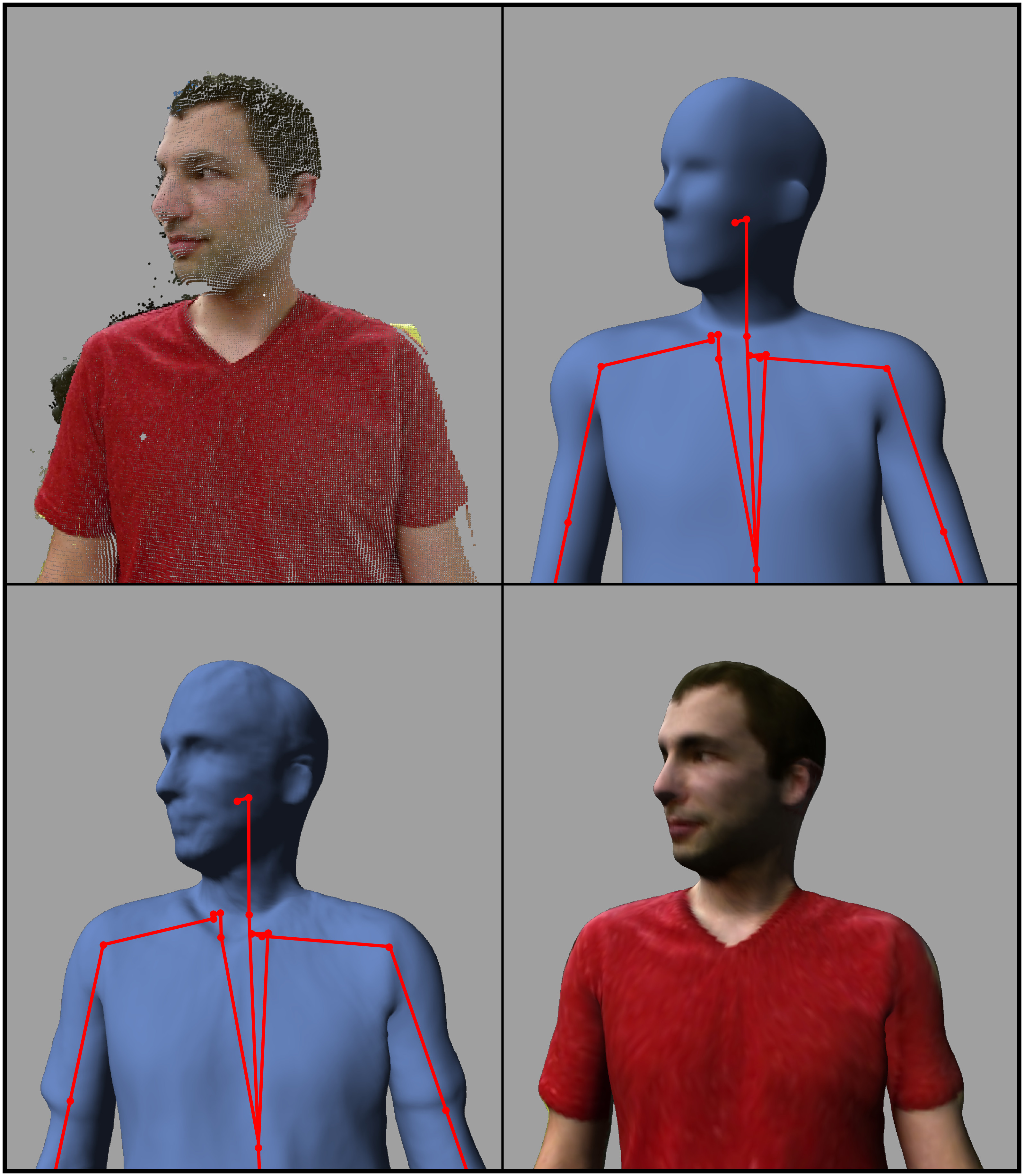
The goal in creating this system is to combine recent advances in dynamic surface reconstruction with fast articulated tracking techniques. Our approach fits a skeletal model and high-resolution polygon mesh to a point cloud. The skeleton is designed to capture the underlying kinematic structure of the subject and estimate it’s large-scale motion, while the polygon mesh captures volume differences between subjects and more complex surface details. This produces both a low-dimensional pose that can be used for gesture and activity recognition, as well as a dense estimation of the surface which can be used for precise physical interaction. Furthermore, because our mesh comes from a predefined template model, it is semantically consistent across capture sessions with different subjects. This means that we can determine not only where the surface of the subject is, but which locations on this surface correspond to specific regions and body parts.

This paper is organized as follows. Section 2 below discusses related work and our relationship to existing approaches. Section 3 describes the details of our model and then Section 4 explains how we fit this model to observations. We then show experimental results in Section 5 and conclude in Section 6.

2 Related Work

2.1 Articulated Tracking and Pose Estimation

Articulated 3D tracking and markerless motion capture has been of interest to the computer vision and robotics communities for several years. The objective of this problem is to estimate the dynamic pose of a complex physical object that can be parameterized using some low-dimensional articulation structure, such as human bodies or hands. Methods for solving this problem can be categorized into discriminative methods which map directly from observations to pose and generative methods which fit a model to the observations, usually based on some previous estimate or initialization.

Discriminative methods ([19, 29, 35]) and hybrid generative methods which incorporate some discriminative component ([14, 20, 32, 37]) have the advantage that they are typically capable of single-frame pose estimation so that they can be initialized automatically and can recover lost tracks easily in a video setting. Recent methods also exist for tracking 3D volumes without skeleton models using discriminative approaches [21, 22], but these also require significant training resources and do not capture high resolution surface detail. In contrast generative methods for articulated model tracking ([6, 15, 16, 18, 33, 39]) have the advantage that they can be readily applied to track new instances or even entirely new classes of models so long as a template is available. For example the discriminative human-body tracker of Shotten et al. [35] required collecting a massive amount of training data, a process which would have to be repeated to track, for example, a dog. In contrast, Ye and Yang showed that their generative technique for tracking human bodies translates directly to tracking a dog by simply creating an appropriate skeletal model [39].

Detecting and tracking human pose from 2D images also has a long and important history ([2, 3, 12, 24]) and has gained significant attention recently with the Microsoft COCO keypoint challenge [27]. While the goal of capturing human pose is similar, this work is somewhat tangential to our method as we aim to produce metrically accurate 3D estimation of pose and shape.

This work presents a new generative model-base tracking technique which estimates fine-grained deformation of the model mesh in addition to the skeletal pose. Many articulated tracking methods, both generative and discriminative, have demonstrated robust performance when tracking subjects such as human hands and bodies that also exhibit non-rigid deformations. However, the deformation is typically not modeled, which means that information about surface shape is not recovered. Some work ([10, 13]) attempt to model this surface shape, but are not capable of online tracking and real time performance. Sometimes, as in the work of Helten et al. [20], the template is initially adapted to a subject based on a set of images of the subject in a canonical pose. Ye and Yang [39] take this a step further by tracking the displacement of individual vertices in their mesh model along the direction of the surface normal. However, our hard association of observed points to model vertices allows us reason the entire mesh and point cloud in real time and therefore track much finer details than is possible with the subsampled soft probabilistic associations of Ye and Yang. This in turn allows us to estimate much more fine-grained deformations when used with a high-resolution mesh, which is evident in the supplementary video.

2.2 Dynamic Surface Reconstruction

Mesh reconstruction of dynamic scenes has also been of interest for some time. For example Li et al. [26] present this as a temporally coherent shape completion on meshes with only partial observability. Recent papers have shown that it is possible to perform 3D mesh reconstruction of dynamic scenes in real time. Initially these methods required a model scanning phase before tracking [40] but later work dropped this requirement [11, 23, 30]. These recent methods work by using reconstruction techniques such as volumetric SDF fusion [8] while simultaneously estimating deformation parameters that warp the reconstructed mesh into its current shape. Reconstruction techniques have the advantage that they can produce accurate shape information with no template and no training data required beforehand. However, starting each reconstruction from scratch results in a lack of correspondence between multiple reconstructions of the same subject. In contrast, we can identify correspondences through our template model within and across video sequences. Furthermore, non-rigid reconstruction techniques must rely on deformation models that are general enough to capture any possible deformations, from fully non-rigid objects such as towels to skeleton-based models such as human bodies. By making use of model-specific prior knowledge, our technique is able to track the majority of the motion in a much lower dimensional pose space, making the optimization more efficient as well as provide the resulting pose as useful additional data.

3 Method: Template Model

Similar to Ye and Yang [39] and Schmidt et al. [33] our technique uses an iterative gradient-based approach to fit a kinematics model to the observed data. We assume that the tracking sequence starts with an initial estimate of the skeletal pose. From that initialization, we iteratively optimize the pose to fit each incoming frame and then use a second optimization to update the vertex positions of a triangle mesh representing the object’s surface. Section 3.1 explains the kinematic structure of our skeleton, while 3.2 and 3.3 detail the model’s shape representation. After this, Section 4 explains the optimization processes used to fit this model to live data.

3.1 Dual Quaternion Kinematic Structure

Our model consists of a skeleton with an attached mesh. The skeleton is made of link frames connected by hinge (rotation) and prismatic (translation) joints. While our human model is primarily made up of hinge joints, we use some prismatics to allow subtle stretching in order to fit subjects with varying proportions and correct for subtle modeling or joint placement errors. Joints such as the shoulder with more than one rotational degree of freedom are represented as multiple hinge joints in succession. The kinematic hierarchy of our human model is shown in Figure 2.

We use the dual quaternion parameterization of SE(3), originally proposed by Clifford [7], to represent the position and orientation of each link in the hierarchy. While this representation may be less familiar, Kavan et al. [25] has shown that it can be used to provide superior performance for smooth mesh attachment. This is discussed later in Section 3.2. Dual quaternions consist of two quaternions of the form $H=q_{r}+q_{d}\epsilon$. Here $\epsilon$ refers to Clifford’s dual unit which satisfies $\epsilon^{2}=0$. The first quaternion $q_{r}$ is referred to as the real part and represents the rotational component of the transformation while $q_{d}$ is the dual part and represents translation. For the sake of space, we omit a thorough coverage of the mathematical details and instead refer readers to [9].

Figure 2: The joint layout of our model.

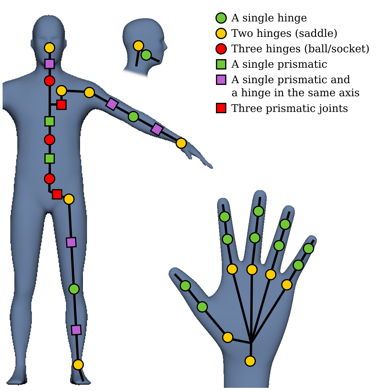
Hinge joints are parameterized by a unit axis $z\in\mathbb{S}^{2}$, and an angle value $\theta\in\mathbb{R}$. Prismatic joints are similarly parameterized by a unit axis $z\in\mathbb{S}^{2}$ and a translation value $\theta$. In our model, the axes $z$ are fixed while $\theta$ changes over time to represent the model pose. Using dual quaternions, a hinge transformation $H_{h}(\theta;z)$ representing a rotation by $\theta$ about a fixed axis $z$ has the form:

$$H_{h}(\theta;z)=\cos(\theta/2)+(z_{x}i+z_{y}j+z_{z}k)\sin(\theta/2)+0\epsilon$$ (1)

A prismatic transform representing a translation by $\theta$ along an axis $z$ can be constructed as:

$$H_{p}(\theta;z)=1+(z_{x}i+z_{y}j+z_{z}k)\frac{\theta}{2}\epsilon$$ (2)

We also store a fixed offset $H_{\mathcal{P}(j),j}\in SE(3)$ between each joint and the link’s origin. This allows us to specify a pivot point and realign the axes if convenient. The link frames are arranged in a hierarchy so we can compute the offset between the world frame and any link frame using the recursive definition:

$$H_{0,j}=H_{0,\mathcal{P}(j)}H_{\mathcal{P}(j),j}H_{j}$$

where $H_{0,0}$ is the identity matrix, $H_{j}$ is the joint transform connecting link $j$ to its direct parent $\mathcal{P}(j)$, and is either a hinge or prismatic joint.

3.2 Surface Representation and Smooth Skinning

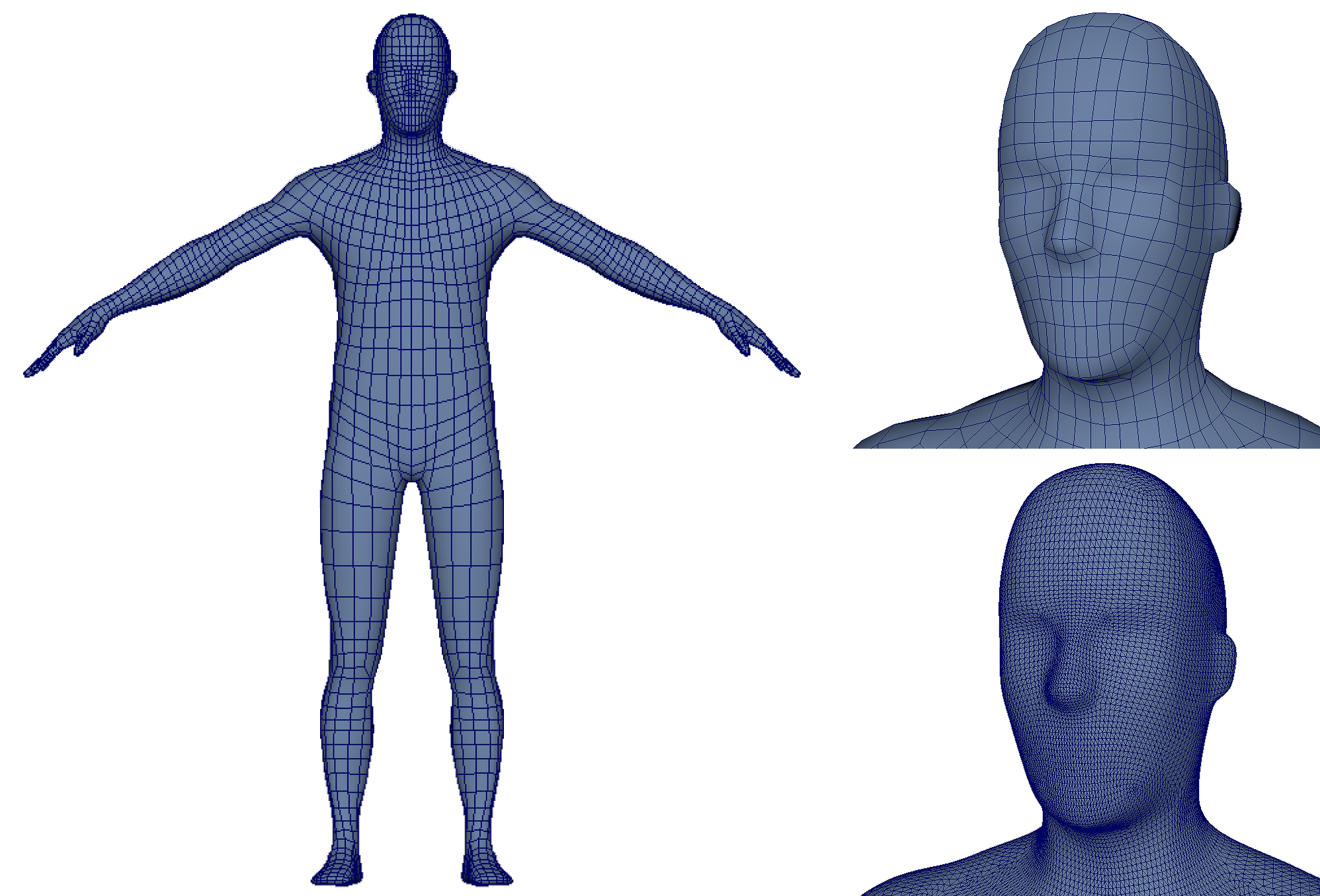
The model’s surface is represented as a high resolution triangle mesh. Unlike the kinematic skeleton, we do not assume any initial estimate of this mesh and initialize it to a smooth default shape shown in figure 3. This mesh consists of set of 3D vertex positions $V=\left\{v_{1}\ldots v_{|V|}\right\},\ v_{i}\in\mathbb{R}^{3}$ as well as a triangle list $F$. Each triangle is represented as a set of three integers referencing vertex indices $F=\left\{f_{1}\ldots f_{|F|}\right\},\ f_{k}\in\mathbb{Z}^{3}$. This way the model can transform the mesh by updating the vertex positions while leaving the face list fixed. The mesh is attached to the skeleton using dual quaternion skinning [25]. This provides a way to smoothly blend the influence of links between different regions of the mesh. Dual quaternion skinning requires a bind pose $H_{0,j}^{0}$ for the skeleton link frames, as well as a weight matrix $\Omega$. The bind pose represents the pose for which the kinematic skeleton matches the default pose of the mesh. We build our skeleton so that the pose in which $\theta=0$ for all joints is the bind pose. The weight matrix describes the influence of each frame on each vertex. Each column $\omega_{i}$ corresponding to vertex $i$ is constrained such that

$$\omega_{i}\in\left[0,1\right]^{|L|},\ \sum_{j=1}^{|L|}\omega_{ij}=1$$

where $|L|$ is the number of skeleton links. Most vertices are weighted to only one or two joints, so we limit the number of non-zero entries in each $\omega_{i}$ to be four and use a sparse representation to store this data in order to limit memory overhead.

Figure 3: Our human body mesh. The left and top right show the low resolution version while the bottom right shows the smoothed high resolution version.

Given this information the skinning function transforms a vertex by computing the offset between the bind pose and the current pose of each frame and then constructing a linear blend $H_{i\Sigma}$ of these offsets for each vertex $v_{i}$ based on the weights.

$$H_{i\Sigma}=\left(\sum_{j=1}^{|L|}H_{0,j}\left(H^{0}_{0,j}\right)^{-1}\omega_{ij}\right)$$ (3)

The skinned vertex position $v_{i}$ can be computed by multiplying this transformation by the vertex position in the default model $v^{0}_{i}$.

$$v_{i}=H_{i\Sigma}v^{0}_{i}$$ (4)

3.3 Dynamic Shape Parameters

Dynamic shape deformation is represented by a set of warp offsets $\Phi$ containing a three vector $\phi_{i}\in\mathbb{R}^{3}$ for each vertex describing a translation away from it default position. We can augment Equation 4 above to compute the warped position $v_{i}$:

$$v_{i}=H_{i\Sigma}(v^{0}_{i}+\phi_{i})$$ (5)

In order to capture high frequency shape details, the mesh necessarily contains a very large number of vertices and triangles. Unfortunately large meshes are unwieldy and it can be difficult to generate the skin weights for them effectively. To avoid this we worked with a low resolution polygon mesh containing 3,460 vertices and 3,476 faces. We then generated a high resolution version automatically using two iterations of Catmul-Clark subdivision [4]. After triangulating the resulting quadrilaterals, this resulted in a mesh with 55,474 vertices and 110,994 triangles. Figure 3 shows the low resolution and high resolution meshes. We also generated high resolution skin weights from the low resolution mesh by interpolating them using the same scheme that Catmul-Clark subdivision uses to interpolate vertex positions.

The low resolution mesh originated from a human model from the website CG Trader [5] by the NoneCG group [31] and was used with permission. We heavily modified this mesh and constructed the skeleton hierarchy and skin weights by hand using Autodesk’s Maya software [1].

4 Method: Optimization

Our model fitting approach alternates between optimizing the skeleton pose and the dynamic warp parameters. Section 4.1 explains the residual term we use for fitting while Section 4.2 and 4.3 discuss kinematic optimization and shape optimization respectively.

4.1 Data Association and Residual Term

Given the model described in Section 3 the task of estimating pose and shape requires estimating the joint angles $\Theta$ and the vertex offsets $\Phi$. This is achieved by first generating a residual term describing the offset between the model and the observations, computing the derivative of that residual with respect to the parameters $\Theta$ and $\Phi$ and then solving a linear system to compute an update that reduces the residual.

Our observations take the form of a point cloud $P=\left\{p_{1}\ldots p_{|P|}\right\}\ p_{k}\in\mathbb{R}^{3}$. Because we use a depth camera to capture these point clouds, each point corresponds to a pixel in a two-dimensional grid. Data association techniques are an important differentiating factor in template based trackers. Ye and Yang [39] use a Gaussian Mixture Model with centroids at the mesh vertex positions to explain the data. While they report that this performs well, this computation is expensive and requires that they subsample their mesh and point cloud when computing the association. Given our high resolution model and our goal of accurate detailed shape estimation, this method would not be feasible in our system. Schmidt et al. [33] use signed distance functions generated from rigid link geometry to compute association. Unfortunately this is also infeasible in our case because we use a single non-rigid mesh to represent the entire subject. Computing a new signed distance function for this mesh for every optimization update would be too slow for our purposes.

Instead of the methods above, we use projective data association that utilizes the grid structure of the point cloud to perform nearest neighbor search. We start by projecting each three dimensional vertex onto the image plane and placing them into buckets corresponding to pixels. We then iterate through all points in the observed point cloud and exhaustively search the buckets in a window around the corresponding pixel for the closest vertex, ignoring anything that is farther away than a cutoff threshold. This guarantees that the closest vertex will be found as long as the window size is chosen correctly relative to the subject’s minimum distance to camera.

At this point it is possible that many point cloud observations have been assigned to the same vertex, so we average the three dimensional offset between the vertex and each point that has been assigned to it. We then compute a point plane residual using this offset and the model’s vertex normal [6]. If we let $N=\left\{n_{1}\ldots n_{|V|}\right\}$ be the vertex normals, and $\widetilde{P}=\left\{\widetilde{p}_{1}\cdots\widetilde{p}_{|V|}\right\}$ be the average of the observation points for which each vertex in $V$ is the closest, the residual term for each vertex is

$$r_{i}=n_{i}^{T}(\widetilde{p}_{i}-v_{i})$$ (6)

The goal of our optimization procedure is to reduce the sum of the squares of these residual terms. In many ways this is a simpler and more direct association technique than that used by Ye and Yang and Schmidt et al. Indeed, as we show in Section 5, we find that it does not perform as well on noisy low resolution sequences such as the EVAL dataset. However on high resolution sequences from a modern time of flight sensor this is more than adequate and has the advantage that it is extremely fast to compute and does not require any complex data structures. This allows us to operate on a very high resolution mesh in real time, which was not possible with previous approaches.

4.2 Kinematic Optimization

The residual term in Equation 6 is a function of the vertex positions $V$ and the position of each vertex is a function of the skeleton pose $\Theta$, the bind pose $H^{0}$, the default mesh vertices $V^{0}$, the vertex offsets $\Phi$ and the skin weights $\Omega$. This means we can optimize the skeleton pose by computing the gradient of the residual with respect to the joint values $\Theta$ and using damped least squares [28] to take an optimization step that reduces the sum of the squares of these residuals. This requires a Jacobian expressing the derivative of the residual $r_{i}$ with respect to the joint angles $\Theta$. For a single vertex we can write this as:

$$\frac{\partial r_{i}}{\partial\Theta}=\frac{\partial r_{i}}{\partial v_{i}}\frac{\partial v_{i}}{\partial\Theta}$$

Because we use point-plane error, the derivative of the residual with respect to each component of the vertex position is simply the vertex normal. The derivative of the vertex position with respect to the skeleton pose $\Theta$ is more complex, but can still be computed analytically. Recall that the skinning operation transforms a model vertex from its offset mesh position $(v^{0}_{i}+\phi_{i})$ to it’s posed position $v_{i}$ by multiplying it by the blended dual quaternion $H_{i\Sigma}$ from Equation 3. We can use $H_{i\Sigma}$ and $H_{j\Delta}=H_{0,j}\left(H^{0}_{0,j}\right)^{-1}$ as intermediate variables and write:

$$\frac{\partial v_{i}}{\partial\Theta}=\frac{\partial v_{i}}{\partial H_{i\Sigma}}\frac{\partial H_{i\Sigma}}{\partial H_{\Delta}}\frac{\partial H_{\Delta}}{\partial\Theta}$$

The first term describes how the three dimensional vertex position $v_{i}$ changes with respect to the eight-dimensional blended dual quaternions $H_{i\Sigma}$ as a 3 by 8 matrix.

$H_{i\Sigma}$ is a linear combination of the link offsets $H_{\Delta}$ for vertex $i$ using the $\Omega$ weight matrix. This means that the weight matrix can be used directly to construct $\partial H_{i\Sigma}/\partial H_{\Delta}$ as an $8$ by $8|L|$ matrix. Each $8\times 8$ block is simply the identity matrix scaled by $\omega_{ij}$.

Because of the hierarchical nature of the skeleton, a single link can be influenced by several $\theta$ values. For example the spine, shoulder and elbow joints will all influence the transform of the hand link. Even though we restrict $\omega$ so that only four frames can influence a single vertex, those four frames may be influenced by many joints in the kinematic hierarchy, which means that the $\partial H_{\Delta}/\partial\Theta$ matrix is relatively dense. If $\theta_{k}$ is an ancestor of link $j$ in the hierarchy, we can compute a block of this matrix corresponding to $H_{j\Delta}$ and $\theta_{k}$ as

$$H_{0,\mathcal{P}(k)}H_{\mathcal{P}(k),k}\frac{\partial H_{k}}{\partial\theta_{k}}H_{k,j}H_{j\Delta}$$

Otherwise if $\theta_{k}$ is not an ancestor link $j$ then this block will be zero. If $\theta_{k}$ corresponds to a prismatic transform from Equation 2, its derivative is

$$\frac{\partial H_{k}}{\partial\theta_{k}}=\frac{(z_{x}i+z_{y}j+z_{z}k)}{2}\epsilon$$

If $\theta_{k}$ corresponds to a hinge transform from Equation 1, the derivative is

$$\frac{\partial H_{k}}{\partial\theta_{k}}=\frac{(z_{x}i+z_{y}j+z_{z}k)\cos(\theta_{k}/2)-\sin(\theta_{k}/2)}{2}$$

The damped least squares method involves solving

$$(J^{T}J+\lambda_{k}\text{diag}(J^{T}J))x=J^{T}r$$

for x. The full $J^{T}J$ and $J^{T}r$ matrices can be computed as

$$J^{T}J=\sum_{i=1}^{|V|}\left(\frac{\partial r_{i}}{\partial\Theta}\right)^{T}\frac{\partial r_{i}}{\partial\Theta}$$ (7)

$$J^{T}r=\sum_{i=1}^{|V|}\left(\frac{\partial r_{i}}{\partial\Theta}\right)^{T}r_{i}$$ (8)

For a high resolution mesh, this can be efficiently computed on a GPU by computing each $(\partial r_{i}/\partial\Theta)^{T}\partial r_{i}/\partial\Theta$ in parallel and using atomic operations to sum them.

As a final addition, we add a default pose prior that penalizes the squared value of $\theta$ for all joints. This encourages the optimization to relax towards the default pose when there are few observations for a particular link and avoid joint limits. The values of $\Theta$ are multiplied by a diagonal matrix $S$ that weights each joint by the number of vertices it influences. This prevents the penalty from overwhelming smaller joints that might not get enough observations to overcome it otherwise. To do this we augment Equations 7 and 8:

$$J^{T}J=\sum_{i=1}^{|V|}\left(\frac{\partial r_{i}}{\partial\Theta}\right)^{T}\frac{\partial r_{i}}{\partial\Theta}+(\lambda_{s}S)^{2}$$

$$J^{T}r=\sum_{i=1}^{|V|}\left(\frac{\partial r_{i}}{\partial\Theta}\right)^{T}r_{i}+(\lambda_{s}S)^{2}\Theta$$

The $(J^{T}J+\lambda_{k}\text{diag}(J^{T}J))$ matrix is positive semi-definite, meaning the system can be solved efficiently using Cholesky decomposition [17] implemented in CUDA. Once $x$ has been computed it is subtracted from the current pose $\Theta$ and the process is repeated. As the pose is updated, the smooth skinning operation pulls the mesh into place and provides an initialization point for the shape optimization. In practice we have found that ten to fifteen iterations of this optimization for each incoming frame is sufficient to match the pose of the target and keep the system running at real time frame rates. The top right frame of Figure 1 shows the result of fitting the kinematic model with the default mesh onto a point cloud without additional shape estimation.

4.3 Shape Optimization

Once the pose has been fit, we update the shape deformation parameters $\Phi$. These consist of a vector $\phi_{i}\in\mathbb{R}^{3}$ for each vertex. The shape optimization uses the residual from Equation 6 but incorporates additional regularization terms.

$$\hat{r}_{i}=r_{i}+\lambda_{\phi}||\phi_{i}||_{2}^{2}+\lambda_{\mathcal{N}}\sum_{n\in\mathcal{N}(i)}||\phi_{i}-\phi_{n}||^{2}_{2}$$ (9)

The term weighted by $\lambda_{\phi}$ penalizes magnitudes of the $\Phi$ vectors and helps prevent the mesh from drifting off the skeleton. The term weighted by $\lambda_{\mathcal{N}}$ penalizes the difference between each $\phi_{i}$ and those of a set $\mathcal{N}(i)$ of neighboring vertices in the default mesh. We typically use the four closest vertices as the neighborhood. This helps prevent surface discontinuities and creases.

As before we compute the derivative of this residual for each vertex $v_{i}$ with respect to the elements of $\Phi$, but make one important simplifying approximation. Technically the neighborhood smoothing term introduces interdependence between each $\phi_{i}$ and its neighbors, but in order to simplify the computation we treat each $\phi_{i}$ as if it were independent. This means that instead of solving one large but sparse $3|V|$ by $3|V|$ linear system $(\partial\hat{r}/\partial\Phi)$ we break it up into a separate 3 by 3 linear system for each vertex $(\partial\hat{r}_{i}/\partial\phi_{i})$ and solve them in parallel. This means we can compute a Jacobian $J_{i}$ for each vertex as

$$J_{i}=\frac{\partial\hat{r}_{i}}{\partial\phi_{i}}=\frac{\partial r_{i}}{\phi_{i}}+2\lambda_{\phi}\phi_{i}+2\lambda_{\mathcal{N}}\sum_{n\in\mathcal{N}(i)}(\phi_{i}-\phi_{n})$$

Once we have computed our warp Jacobian $J_{i}$ we compute $J_{i}^{T}J_{i}$ as before and solve

$$(J_{i}^{T}J_{i}+\lambda_{w}\text{diag}(J_{i}^{T}J_{i}))x=J_{i}^{T}\hat{r}_{i}$$

for $x$, and subtract it from $\phi_{i}$. This means we have a linear system of three equations with three unknowns for each vertex, which we solve in batch on a GPU, assigning one linear system to each thread. The bottom left frame of Figure 1 shows the result of the shape deformation after the kinematic pose has been fit. In practice only two iterations of shape refinement are necessary for each incoming video frame.

Figure 4: The performance of our method in various conditions on our dataset along with the method of Schmidt et al. [33] for comparison. Each curve shows the percentage of joint positions in these sequences that are within the distance indicated on the x-axis from the ground truth positions. Area under the curve is shown for each plot in parentheses.

5 Experiments

Figure 5: Our performance on the EVAL dataset compared to Articulated ICP reported by [15], Ganapthi et al.[15], Schmidt et al.[33] and Ye and Yang[39].

There are a number of existing datasets designed to test the capabilities of markerless motion capture systems on point cloud data. The SMMC [14] and EVAL [15] datasets provide depth images along with ground truth pose data. The Personalized Depth Tracker (PDT) dataset [20] contains ground truth information for adapting a mesh shape to different subjects, but is not concerned with estimating shape dynamics over time. Unfortunately the depth information in these datasets was captured with either a first generation Microsoft Kinect in the case of PDT and EVAL or a Swiss Ranger SR4000 in the case of SMMC and does not have enough fidelity to capture high resolution surface details. Specifically in the PDT and EVAL datasets the depth values are discretized to around two centimeter intervals, while the SMMC data is only 176x144 pixels with heavy depth noise. To address this we generated a new dataset of videos captured with the second generation Microsoft Kinect (Kinect One) [34] camera using the open source libfreenect2 drivers [38], but also test on the EVAL dataset for completeness. Finally we also report reconstruction error for our method to quantify improvement over conditions that do not estimate dynamic shape.

The experiments in this paper were performed on a PC running the Ubuntu Linux distribution with a 2.4 GHz Xeon quadcore processor and an Nvidia GeForce 1080 and on a laptop with a 2.6 Ghz Intel i7 and an NVidia Geforce 1070. Both of these machines run our tracker at frame rates faster than 20Hz.

Figure 6: Reconstruction error of our method under various conditions. Area under the curve is listed for each plot in parentheses.

Figure 7: Reconstruction error visualized for a single frame. From left to right: the point cloud, our fully deformed model, our model with $\Phi$ fixed to the best fit at the start frame, the smooth skinned mesh with $\Phi=0$ and rigid link geometry.

Figure 8: A collection of still frames showing the results of our system. For each pair of images, the left shows the colored point cloud while the right shows our warped output mesh.

5.1 Our Dataset

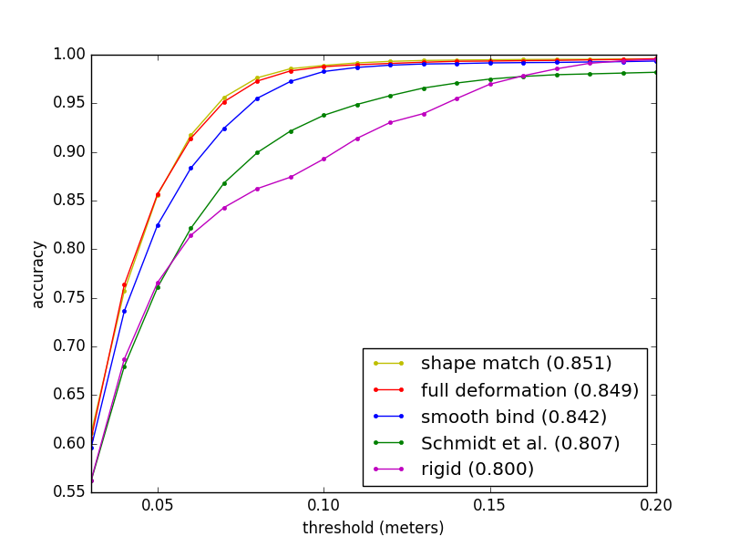
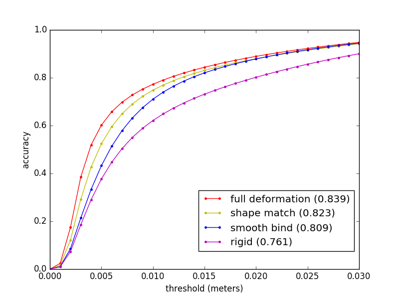
Our dataset consists of four sequences with high quality manually annotated pose information. There are two subjects, each of which has one close sequence from the waist up and one far sequence where the full body is visible. Each sequence contains 300 frames of depth video with a resolution of 512x424 pixels. We label the 3D location of fifteen joints in each frame: the head, torso, pelvis and left/right hip, knee, ankle, shoulder, elbow and wrist. We also annotate when these joints become invisible by either leaving the frame or becoming occluded. We tested our system on these sequences in different conditions to study how different components of our system affect the performance of pose tracking. This includes our full system which estimates dynamic shape on each frame, a shape match mode that estimates shape on the first frame and then freezes the dynamic warp parameters $\Phi$ for the rest of the sequence, a smooth bind mode which does not perform shape estimation at all and only tracks kinematic pose and a separate model made up of rigid mesh segments for each link. We also tested the method of Schmidt et al. [33] on these sequences using an open source implementation provided by the authors. We used our own model with this method for consistency, but had to remove the prismatic joints because they are unsupported. In all other cases, the kinematic hierarchy and joint positions were the same. The rigid segments used when testing Schmidt et al. and our own rigid model were generated by cutting our mesh into multiple disjoint components and filling the resulting holes.

Rather than reporting a precision score using a single threshold to determine correctness as is common practice on the EVAL dataset, we instead plot accuracy as a function of this threshold. Figure 4 shows these results. As can be seen, the dynamic shape estimation and the mode that fits the shape to the first frame perform almost identically, and significantly improve tracking performance compared to other methods. This demonstrates the importance of shape accuracy for template based tracking.

5.2 EVAL Dataset

The EVAL dataset consists of twenty-four RGBD sequences split evenly across three human subjects with varying body proportions. The evaluation criteria is the percentage of frames in which the estimated joint position is within ten centimeters of the ground truth. Because the ground truth data relies on joint locations specific to a particular model, we follow the technique of [39] and use mean-subtraction to find the best placement of the tracked joints relative to our model. Because of the limitations of the depth data pointed out above we disabled the dynamic shape estimation and used a simplified kinematics model and mesh for this experiment.

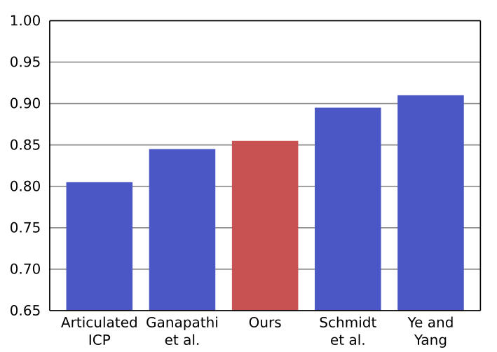
Figure 5 shows our performance compared to the reported scores of other methods. While we do not perform as well as other state of the art techniques, our method was not designed to work with low resolution depth data.

5.3 Shape Fitting

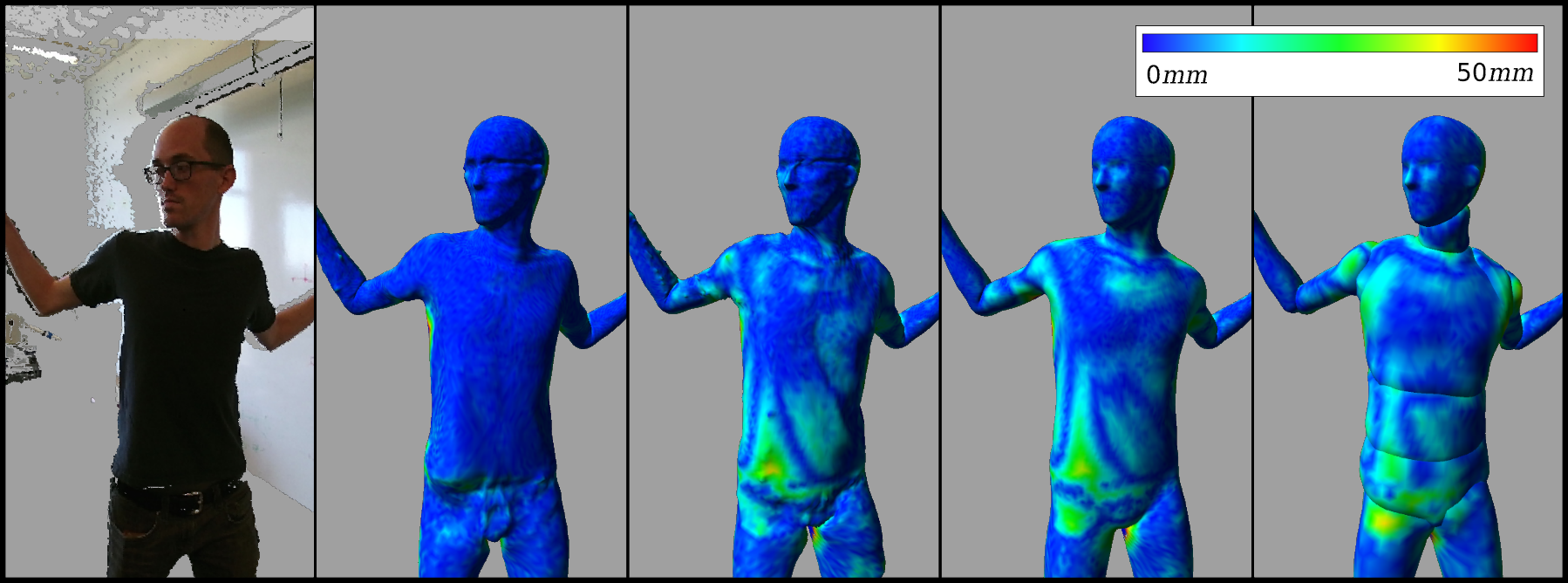
In order to test our dynamic shape estimation, we compute the reconstruction error of our model as the point wise distances between the visible vertices and the nearest point in the observation for each frame in our dataset. We test this under the same conditions that we used to test our pose tracking. Figure 6 shows these results. In this case our dynamic shape fitting offers clear improvements over the other modes. Figure 7 shows a single frame from each mode colored to show reconstruction error.

5.4 Qualitative Results

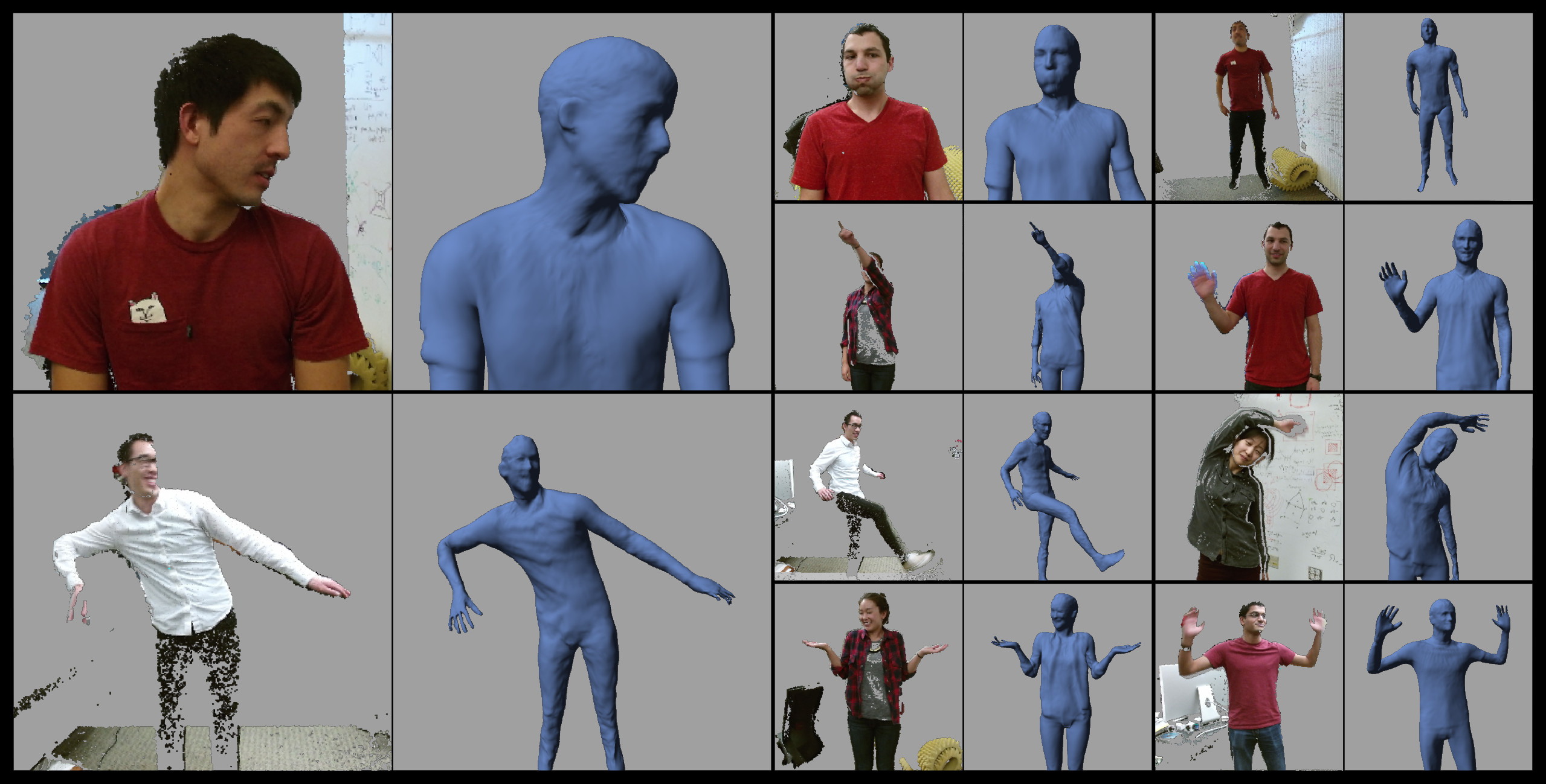
Figure 8 shows ten frames from four male and two female subjects. Each frame has a colored point clouds and the corresponding tracked mesh. In all cases the tracker was given a rough initialization of the subject’s pose at the start of the sequence, and the pose and shape tracked from that point forward. The model was not customized to any of these subjects beforehand except for a single uniform scale parameter which was only approximately estimated based on the subject’s height. This demonstrates the robustness of our model to different of subjects with varying proportions at a range of distances to camera. Detailed surface features are clearly visible in all images showing the visual fidelity of our tracked meshes.

6 Conclusion

We have demonstrated an articulated tracking approach for deformable objects that is able to track humans using a high resolution template mesh. We have shown that it can produce dense and accurate estimation of detailed deformable surfaces in real time. This system also provides useful pose estimates of the model’s kinematic structure for gesture recognition and motion prediction.

This work opens up some important areas of future research. While many figures in this paper feature colored point clouds, our technique does not currently use color information as part of the tracking process. Incorporating color may help the mesh lock on to specific color features and prevent vertices from drifting along the surface of an object. Fine structures such as fingers with many degrees of freedom currently pose a challenge. This is partially due to sensor resolution, but more could be done to regularize their kinematic motion. Taylor er al. [36] show promising results in this direction. Finally this technique can be combined with discriminative detection systems to more easily recover from tracking errors and avoid the need for pose initialization.

References

- [1] Autodesk Incorporated. Maya. URL https://autodesk.com/products/maya/overview.
- Cao et al. [2016] Zhe Cao, Tomas Simon, Shih-En Wei, and Yaser Sheikh. Realtime multi-person 2d pose estimation using part affinity fields. CoRR, abs/1611.08050, 2016.
- Carreira et al. [2016] Joao Carreira, Pulkit Agrawal, Katerina Fragkiadaki, and Jitendra Malik. Human pose estimation with iterative error feedback. In Proceedings of the IEEE Conference on Computer Vision and Pattern Recognition, pages 4733–4742, 2016.
- Catmull and Clark [1978] Edwin Catmull and James Clark. Recursively generated b-spline surfaces on arbitrary topological meshes. Computer-aided design, 10(6):350–355, 1978.
- [5] CG Trader. Cg trader. URL http://www.cgtrader.com/.
- Chen and Medioni [1992] Yang Chen and Gérard Medioni. Object modelling by registration of multiple range images. Image and vision computing, 10(3):145–155, 1992.
- Clifford [1882] William Kingdon Clifford. Mathematical papers. Macmillan and Company, 1882.
- Curless and Levoy [1996] Brian Curless and Marc Levoy. A volumetric method for building complex models from range images. In Proceedings of the 23rd annual conference on Computer graphics and interactive techniques, pages 303–312. ACM, 1996.
- Daniilidis [1999] Konstantinos Daniilidis. Hand-eye calibration using dual quaternions. The International Journal of Robotics Research, 18(3):286–298, 1999.
- De Aguiar et al. [2008] Edilson De Aguiar, Carsten Stoll, Christian Theobalt, Naveed Ahmed, Hans-Peter Seidel, and Sebastian Thrun. Performance capture from sparse multi-view video. In ACM Transactions on Graphics (TOG), volume 27, page 98. ACM, 2008.
- Dou et al. [2016] Mingsong Dou, Sameh Khamis, Yury Degtyarev, Philip Davidson, Sean Ryan Fanello, Adarsh Kowdle, Sergio Orts Escolano, Christoph Rhemann, David Kim, Jonathan Taylor, et al. Fusion4d: Real-time performance capture of challenging scenes. ACM Transactions on Graphics (TOG), 35(4):114, 2016.
- Ferrari et al. [2008] Vittorio Ferrari, Manuel Marin-Jimenez, and Andrew Zisserman. Progressive search space reduction for human pose estimation. In Computer Vision and Pattern Recognition, 2008. CVPR 2008. IEEE Conference on, pages 1–8. IEEE, 2008.
- Gall et al. [2009] Juergen Gall, Carsten Stoll, Edilson De Aguiar, Christian Theobalt, Bodo Rosenhahn, and Hans-Peter Seidel. Motion capture using joint skeleton tracking and surface estimation. In Computer Vision and Pattern Recognition, 2009. CVPR 2009. IEEE Conference on, pages 1746–1753. IEEE, 2009.
- Ganapathi et al. [2010] Varun Ganapathi, Christian Plagemann, Daphne Koller, and Sebastian Thrun. Real time motion capture using a single time-of-flight camera. In Computer Vision and Pattern Recognition (CVPR), 2010 IEEE Conference on, pages 755–762. IEEE, 2010.
- Ganapathi et al. [2012] Varun Ganapathi, Christian Plagemann, Daphne Koller, and Sebastian Thrun. Real-time human pose tracking from range data. In European conference on computer vision, pages 738–751. Springer, 2012.
- Garcia Cifuentes et al. [2016] Cristina Garcia Cifuentes, Jan Issac, Manuel Wüthrich, Stefan Schaal, and Jeannette Bohg. Probabilistic articulated real-time tracking for robot manipulation. IEEE Robotics and Automation Letters (RA-L), 2016.
- Gill and Murray [1974] Philip E Gill and Walter Murray. Newton-type methods for unconstrained and linearly constrained optimization. Mathematical Programming, 7(1):311–350, 1974.
- Grest et al. [2005] Daniel Grest, Jan Woetzel, and Reinhard Koch. Nonlinear body pose estimation from depth images. In Joint Pattern Recognition Symposium, pages 285–292. Springer, 2005.
- Haque et al. [2016] Albert Haque, Boya Peng, Zelun Luo, Alexandre Alahi, Serena Yeung, and Li Fei-Fei. Towards viewpoint invariant 3d human pose estimation. In European Conference on Computer Vision, pages 160–177. Springer, 2016.
- Helten et al. [2013] Thomas Helten, Andreas Baak, Gaurav Bharaj, Meinard Müller, Hans-Peter Seidel, and Christian Theobalt. Personalization and evaluation of a real-time depth-based full body tracker. In 2013 International Conference on 3D Vision-3DV 2013, pages 279–286. IEEE, 2013.
- Huang et al. [2015] Chun-Hao Huang, Edmond Boyer, Bibiana do Canto Angonese, Nassir Navab, and Slobodan Ilic. Toward user-specific tracking by detection of human shapes in multi-cameras. In Proceedings of the IEEE Conference on Computer Vision and Pattern Recognition, pages 4027–4035, 2015.
- Huang et al. [2016] Chun-Hao Huang, Benjamin Allain, Jean-Sébastien Franco, Nassir Navab, Slobodan Ilic, and Edmond Boyer. Volumetric 3d tracking by detection. In Proceedings of the IEEE Conference on Computer Vision and Pattern Recognition, pages 3862–3870, 2016.
- Innmann et al. [2016] Matthias Innmann, Michael Zollhöfer, Matthias Nießner, Christian Theobalt, and Marc Stamminger. Volumedeform: Real-time volumetric non-rigid reconstruction. In Proceedings of the European Conference on Computer Vision (ECCV), 2016.
- Iqbal et al. [2016] Umar Iqbal, Anton Milan, and Juergen Gall. Pose-track: Joint multi-person pose estimation and tracking. CoRR, abs/1611.07727, 2016.
- Kavan et al. [2008] Ladislav Kavan, Steven Collins, Jiří Žára, and Carol O’Sullivan. Geometric skinning with approximate dual quaternion blending. ACM Transactions on Graphics (TOG), 27(4):105, 2008.
- Li et al. [2012] Hao Li, Linjie Luo, Daniel Vlasic, Pieter Peers, Jovan Popović, Mark Pauly, and Szymon Rusinkiewicz. Temporally coherent completion of dynamic shapes. ACM Transactions on Graphics (TOG), 31(1):2, 2012.
- Lin et al. [2014] Tsung-Yi Lin, Michael Maire, Serge Belongie, James Hays, Pietro Perona, Deva Ramanan, Piotr Dollár, and C Lawrence Zitnick. Microsoft coco: Common objects in context. In European conference on computer vision, pages 740–755. Springer, 2014.
- Marquardt [1963] Donald W Marquardt. An algorithm for least-squares estimation of nonlinear parameters. Journal of the society for Industrial and Applied Mathematics, 11(2):431–441, 1963.
- Mehta et al. [2017] Dushyant Mehta, Srinath Sridhar, Oleksandr Sotnychenko, Helge Rhodin, Mohammad Shafiei, Hans-Peter Seidel, Weipeng Xu, Dan Casas, and Christian Theobalt. Vnect: Real-time 3d human pose estimation with a single rgb camera. arXiv preprint arXiv:1705.01583, 2017.
- Newcombe et al. [2015] Richard A Newcombe, Dieter Fox, and Steven M Seitz. Dynamicfusion: Reconstruction and tracking of non-rigid scenes in real-time. In Proceedings of the IEEE conference on computer vision and pattern recognition, pages 343–352, 2015.
- [31] NoneCG. Nonecg. URL http://www.nonecg.com/.
- Plagemann et al. [2010] Christian Plagemann, Varun Ganapathi, Daphne Koller, and Sebastian Thrun. Real-time identification and localization of body parts from depth images. In Robotics and Automation (ICRA), 2010 IEEE International Conference on, pages 3108–3113. IEEE, 2010.
- Schmidt et al. [2014] Tanner Schmidt, Richard Newcombe, and Dieter Fox. Dart: Dense articulated real-time tracking. Proceedings of Robotics: Science and Systems, Berkeley, USA, 2, 2014.
- Sell and O’Connor [2014] John Sell and Patrick O’Connor. The xbox one system on a chip and kinect sensor. IEEE Micro, 34(2):44–53, 2014.
- Shotton et al. [2013] Jamie Shotton, Toby Sharp, Alex Kipman, Andrew Fitzgibbon, Mark Finocchio, Andrew Blake, Mat Cook, and Richard Moore. Real-time human pose recognition in parts from single depth images. Communications of the ACM, 56(1):116–124, 2013.
- Taylor et al. [2016] Jonathan Taylor, Lucas Bordeaux, Thomas Cashman, Bob Corish, Cem Keskin, Toby Sharp, Eduardo Soto, David Sweeney, Julien Valentin, Benjamin Luff, et al. Efficient and precise interactive hand tracking through joint, continuous optimization of pose and correspondences. ACM Transactions on Graphics (TOG), 35(4):143, 2016.
- Tompson et al. [2014] Jonathan Tompson, Murphy Stein, Yann Lecun, and Ken Perlin. Real-time continuous pose recovery of human hands using convolutional networks. ACM Transactions on Graphics (TOG), 33(5):169, 2014.
- Xiang et al. [2016] Lingzhu Xiang, Florian Echtler, Christian Kerl, Thiemo Wiedemeyer, Lars, hanyazou, Ryan Gordon, Francisco Facioni, laborer2008, Rich Wareham, Matthias Goldhoorn, alberth, gaborpapp, Steffen Fuchs, jmtatsch, Joshua Blake, Federico, Henning Jungkurth, Yuan Mingze, vinouz, Dave Coleman, Brendan Burns, Rahul Rawat, Serguei Mokhov, Paul Reynolds, P.E. Viau, Matthieu Fraissinet-Tachet, Ludique, James Billingham, and Alistair. libfreenect2: Release 0.2, April 2016. URL https://doi.org/10.5281/zenodo.50641.
- Ye and Yang [2014] Mao Ye and Ruigang Yang. Real-time simultaneous pose and shape estimation for articulated objects using a single depth camera. In Proceedings of the IEEE Conference on Computer Vision and Pattern Recognition, pages 2345–2352, 2014.
- Zollhöfer et al. [2014] Michael Zollhöfer, Matthias Nießner, Shahram Izadi, Christoph Rehmann, Christopher Zach, Matthew Fisher, Chenglei Wu, Andrew Fitzgibbon, Charles Loop, Christian Theobalt, et al. Real-time non-rigid reconstruction using an rgb-d camera. ACM Transactions on Graphics (TOG), 33(4):156, 2014.