The TRAPPIST-1 system: Orbital evolution, tidal dissipation, formation and habitability

Abstract

We study the dynamical evolution of the TRAPPIST-1 system under the influence of orbital circularization through tidal interaction with the central star. We find that systems with parameters close to the observed one evolve into a state where consecutive planets are linked by first order resonances and consecutive triples, apart from planets c, d and e, by connected three body Laplace resonances. The system expands with period ratios increasing and mean eccentricities decreasing with time. This evolution is largely driven by tides acting on the innermost planets which then influence the outer ones. In order that deviations from commensurability become significant only on $Gy$ time scales or longer, we require that the tidal parameter associated with the planets has to be such that $Q^{\prime}>\sim 10^{2-3}.$ At the same time, if we start with two subsystems, with the inner three planets comprising the inner one, $Q^{\prime}$ associated with the planets has to be on the order (and not significantly exceeding) $10^{2-3}$ for the two subsystems to interact and end up in the observed configuration. This scenario is also supported by modelling of the evolution through disk migration which indicates that the whole system cannot have migrated inwards together. Also in order to avoid large departures from commensurabilities, the system cannot have stalled at a disk inner edge for significant time periods. We discuss the habitability consequences of the tidal dissipation implied by our modelling, concluding that planets d, e and f are potentially in habitable zones.

1 Introduction

The TRAPPIST-1 system is the first transiting planet system found orbiting an ultra-cool M$8V$ dwarf star. Transits of the planets TRAPPIST-1 b, c and d with radii comparable to the earth were reported by Gillon et al. (2016). Subsequently the number of transiting planets was increased to seven by Gillon et al. (2017). They noted that the inner six planets were in near commensurable orbits and thus form a resonant chain. Luger et al. (2017) noted the possibility of three body resonances amongst sets of consecutive triples and postulated the existence of a three body resonance between planets f, g and h, which led to the specification of a 3:2 resonance between planets g and h, which enabled a firm detection of the period of planet h. They also indicated the existence of a three body Laplace resonance between planets b, c and d, which can be thought of resulting from 3:2 commensurabilities between the pair b and c and between the pair c and d, even though departures from these first order commensurabilities are large. Allowing for this situation, all consecutive pairs are in or affected by first order commensurabilities (see table 1 below).

The configuration of TRAPPIST-1 is indicative that it was formed by inward migration through a protoplanetary disc as resonant chains form naturally in that scenario (eg. Cresswell & Nelson 2006). In addition they are close enough to the central star for it to be possible that tidal interaction has affected the dynamics and led to evolution of successive period ratios (eg. Papaloizou 2011). As noted by Gillon et al. (2017) conditions are such that planets d - g may have liquid water on their surfaces and therefore possibly be habitable. All of these features make the TRAPPIST-1 system one of topical interest.

In this paper we study the dynamics of the TRAPPIST-1 system taking into account tidal interaction with the central star that leads to orbital circularization. This allows us to obtain constraints on the strength of this interaction that come about in order to avoid significant departures from the present configuration over its estimated lifetime. We also consider the consequences of the tidal dissipation that could occur when these constraints are adhered to for the habitability of the planets in the system.

As the system is likely to have reached its present configuration as a result of migration from larger distances in a protoplanetary disc, we construct models for this process that adopt the expected scaling for migration rates through the disc. In particular we consider the issue as to whether the system can have migrated as a unit or separated into two detached subsystems. In the latter case we perform simulations to determine under what conditions evolution under tidal interaction with the central star can have restored the system to its current form.

The plan of this paper is as follows. In Section 2 we describe the physical model and basic equations we use to describe the planetary system moving under its mutual gravitational interactions together with forces due to tidal interaction with the central star and interaction with a protoplanetary disc if present. In Section 3 we give an analytical description of a system of N planets, in which consecutive groups of three planets are linked by three body Laplace resonances, which expands under the action of tidal circularization which occurs while the system conserves angular momentum. This expansion causes a secular increase of the period ratios seen in simulations. In Section 3.1 the treatment is extended to consider two connected subsystems.

We go on to describe our numerical simulations of two model systems, A, and B, with orbital parameters close to those of the present TRAPPIST-1 system, but different masses in Section 4. We give results in Section 4.1 that show that the evolution in general sets up a system of three body Laplace resonances with related pairs of first order resonances connecting all consecutive sets of three planets, apart from planets c, d and e for different values of their associated tidal parameter $Q^{\prime}.$ We go on to consider simulations for which either the inner three planets or the inner two were split off from the rest and moved to smaller radii, so forming a separate subsystem in section 4.4. These indicate that this subsystem can merge with that formed by the outer planets to form a system like TRAPPIST-1.

In order to investigate the origin of the system we perform simulations of the planets migrating in a protoplanetary disc in Section 5. We also consider the maintenance of commensurabilities, the evolution of period ratios and the effects of disc dispersal on resonant chains. We discuss the possible effects of the tidal dissipation inferred from our simulations on habitability in Section 6. Finally we summarise and discuss our results in Section 7.

2 Model and basic equations

We consider a system of $N$ planets moving under their mutual gravitational attraction and that due to the central star. The equations of motion are:

$${d^{2}{\bf r}_{i}\over dt^{2}}=-{GM{\bf r}_{i}\over|{\bf r}_{i}|^{3}}-\sum_{j=1\neq i}^{N}{Gm_{j}\left({\bf r}_{i}-{\bf r}_{j}\right)\over|{\bf r}_{i}-{\bf r}_{j}|^{3}}-{\bf\Gamma}+{\bf\Gamma}_{m,i}+{\bf\Gamma}_{e,i}+{\bf\Gamma}_{r,i}\;,$$ (1)

where $M$, $m_{i},$ $m_{j},$ ${\bf r}_{i}$ and ${\bf r}_{j}$ denote the mass of the central star, the mass of planet $i,$ the mass of planet $j,$ the position vector of planet $i$ and the position vector of planet $j,$ respectively. The enumeration is such that $i=1$ corresponds to the innermost planet and $i=N$ to the outermost planet. The acceleration of the coordinate system based on the central star (indirect term) is:

$${\bf\Gamma}=\sum_{j=1}^{N}{Gm_{j}{\bf r}_{j}\over|{\bf r}_{j}|^{3}}.$$ (2)

Migration torques can be included through, ${\bf\Gamma}_{m,i},$ which takes the form (see eg. Terquem & Papaloizou 2007)

$${\bf\Gamma}_{m,i}=\frac{{\bf r}_{i}\times\left({\bf r}_{i}\times d{\bf r}_{i}/dt\right)}{3|{\bf r}_{i}|^{2}t_{mig,i}}$$ (3)

where $t_{mig,i}$ is defined to be the inward migration time for planet $i,$ being the characteristic time scale on which the mean motion increases. Tidal interaction with the central star is dealt with through the addition of a frictional damping force taking the form (see eg. Papaloizou & Terquem 2010)

$${\bf\Gamma}_{e,i}=-\frac{2}{|{\bf r}_{i}|^{2}t_{e,i}}\left(\frac{d{\bf r}_{i}}{dt}\cdot{\bf r}_{i}\right){\bf r}_{i}$$ (4)

where $t_{e,i}$ is the time scale over which the eccentricity of an isolated planet damps. Thus it is the orbital circularization time (see below). Note that in this formulation, eccentricity damping acts through radial velocity damping, which is associated with energy loss at constant angular momentum. Thus it causes both the semi–major axis and the eccentricity to decrease. We write

$$\frac{1}{t_{e,i}}=\frac{1}{t_{e,i}^{d}}+\frac{1}{t_{e,i}^{s}},$$ (5)

where $t_{e,i}^{d}$ and $t_{e,i}^{s}$ are the damping timescales due to the protoplanetary disc and tidal circularization due to the central star respectively. Relativistic effects may be included through ${\bf\Gamma}_{r,i}$ (see Papaloizou & Terquem 2001).

2.1 Time scale for orbital migration

It is likely that systems of close orbiting planets were not formed in their present locations but were formed further out and then migrated inwards while the protoplanetary disc was still present (see eg. Papaloizou & Terquem 2006; Baruteau et al. 2014 for reviews). In particular convergent disc migration readily produces multiple systems in resonant chains of the type observed in TRAPPIST-1 (eg. Cresswell & Nelson 2006; Papaloizou & Terquem 2010). However, if they form relatively close to resonance with migration operating only for a limited time, the system as a whole may undergo little net radial migration. But note that a rapid removal of the disc, due to for example photoevaporation, may cause disruption of the resonances (eg. Terquem 2017).

In this paper we assume that the system was formed near to its current state and examine the role of tides due to the central star in cementing the resonances and causing subsequent evolution. This leads to constraints on the strength of the tides. We also consider properties of the protoplanetary disc, and the time scale for its dispersal, that ensure the system is not immediately disrupted.

2.2 Time scale for orbital circularization due to tides from the central star

The circularization timescale due to tidal interaction with the star was obtained from Goldreich & Soter (1966) in the form

$$t_{e,i}^{s}=763000Q^{\prime}\left(\frac{M_{\oplus}}{m_{i}}\right)^{2/3}\left(\frac{M_{\odot}}{M}\right)^{1.5}\left(\frac{{\overline{\rho}}_{i}}{{\overline{\rho}}_{\oplus}}\right)^{5/3}\left(\frac{20a_{i}}{1AU}\right)^{6.5}y.$$

$$\equiv 763000Q^{\prime}\left(\frac{m_{i}}{M_{\oplus}}\right)\left(\frac{M_{\odot}}{M}\right)^{1.5}\left(\frac{R_{\oplus}}{R_{p,i}}\right)^{5}\left(\frac{20a_{i}}{1AU}\right)^{6.5}y.$$ (6)

where $a_{i}$ is the the semi–major axis of planet $i,$ $R_{p,i}$ is its radius and ${\overline{\rho}}_{i}$ is its mean density. The quantity $Q^{\prime}=3Q/(2k_{2}),$ where $Q$ is the tidal dissipation function and $k_{2}$ is the Love number. For solar system planets in the terrestrial mass range, Goldreich & Soter (1966) give estimates for $Q$ in the range 10–500 and $k_{2}\sim 0.3$, which correspond to $Q^{\prime}$ in the range 50–2500. However, the value of $Q$ is expected to be a function of tidal forcing frequency and temperature that could attain a minimum value $\sim 1$ at the solidus temperature (see Ojakangas & Stevenson 1986 and references therein). Although $Q^{\prime}$ is very uncertain for extrasolar planets, we should note that $Q$ may be of order unity under early post formation conditions if they result in a planet being near to the solidus temperature. We remark that when circularization operates, the rate of energy dissipation produced in planet $i,$ with orbital energy $E_{i},$ is given by (see Papaloizou & Terquem 2010):

$$\frac{dE_{i}}{dt}=\frac{2e_{i}^{2}E_{i}}{t_{e,i}^{s}}.$$ (7)

For the low mass planets considered here, we neglect tides induced on the central star as these cannot transfer a significant amount of angular momentum (see eg. Barnes et al. 2009a; Papaloizou & Terquem 2010). Accordingly the orbital angular momentum and inclination are not changed by the tidal interaction.

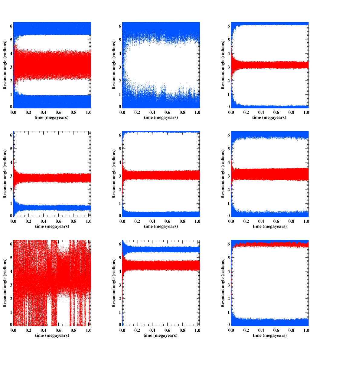
Figure 1: The evolution of the seven planet system with $Q^{\prime}=Q_{0}^{\prime}=0.122127$ but tidal dissipation applied only to the innermost two planets and case A masses, resonant angles. The uppermost left panel shows the resonant angles $3\lambda_{2}-2\lambda_{1}-\varpi_{2}$ (red curve) and $3\lambda_{2}-2\lambda_{1}-\varpi_{1}$ (blue curve). The uppermost middle panel shows the resonant angle $3\lambda_{3}-2\lambda_{2}-\varpi_{2}$ and the uppermost right panel shows the resonant angles $3\lambda_{4}-2\lambda_{3}-\varpi_{4}$ (red curve) and $3\lambda_{4}-2\lambda_{3}-\varpi_{3}$ (blue curve). The left panel in the central row shows the resonant angles $3\lambda_{5}-2\lambda_{4}-\varpi_{5}$ (red curve) and $3\lambda_{5}-2\lambda_{4}-\varpi_{4}$ (blue curve). The middle panel in the central row shows the resonant angles $4\lambda_{6}-3\lambda_{5}-\varpi_{6}$ (red curve) and $4\lambda_{6}-3\lambda_{5}-\varpi_{5}$ (blue curve). The right panel in the middle row shows the resonant angles $3\lambda_{7}-2\lambda_{6}-\varpi_{7}$ (red curve) and $3\lambda_{7}-2\lambda_{6}-\varpi_{6}$ (blue curve). The lowermost left panel shows the resonant angle $5\lambda_{3}-3\lambda_{2}-2\varpi_{3}.$ The lowermost middle panel shows the resonant angles $2\lambda_{6}-\lambda_{4}-\varpi_{6}$ (red curve) and $2\lambda_{6}-\lambda_{4}-\varpi_{4}$ (blue curve). The lowermost right panel shows the resonant angles $2\lambda_{7}-\lambda_{5}-\varpi_{7}$ (red curve) and $2\lambda_{7}-\lambda_{5}-\varpi_{5}$ (blue curve).

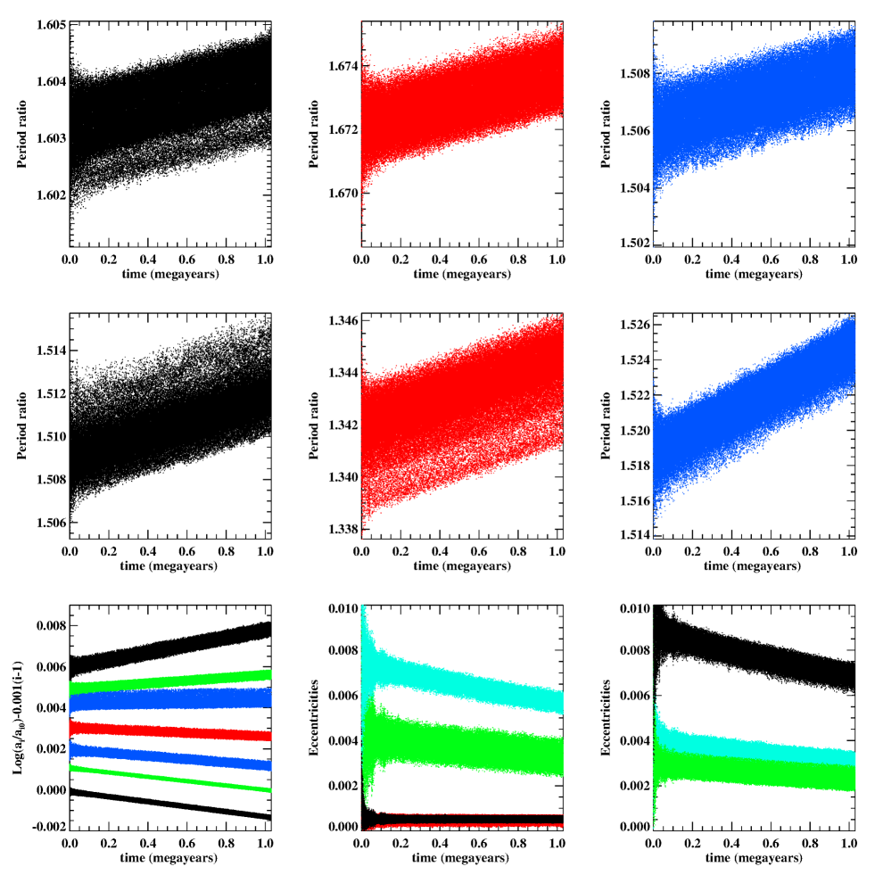
Figure 2: Results for $Q^{\prime}=Q^{\prime}_{0}$ but tidal dissipation applied only to the innermost two planets and case A masses, period ratios and eccentricities. The uppermost left panel shows the period ratio $P_{2}/P_{1}.$ The uppermost middle panel shows the period ratio $P_{3}/P_{2}.$ the uppermost right panel shows the period ratio $P_{4}/P_{3}.$ The left panel in the central row shows the period ratio $P_{5}/P_{4}.$ The middle panel in the central row shows the period ratio $P_{6}/P_{5}.$ The right panel in the middle row shows the period ratio $P_{7}/P_{6}.$ The lowermost left panel shows $\log(a_{i}/a_{i0})-0.001(i-1)$ for $i=1-7,$ where $a_{i0}$ is the initial value of the semi-major axis of planet $i.$ Planets $1-7$ correspond to curves taking on monotonically increasing values ranging from lowermost to uppermost. The lowermost middle panel shows the eccentricities, $e_{1}$ (black curve), $e_{2}$ (red curve), $e_{3}$(green curve) and $e_{4}$ (light blue curve). The lowermost right panel shows the eccentricities, $e_{5}$ (black curve), $e_{6}$(light blue curve) and $e_{7}$ (green curve).

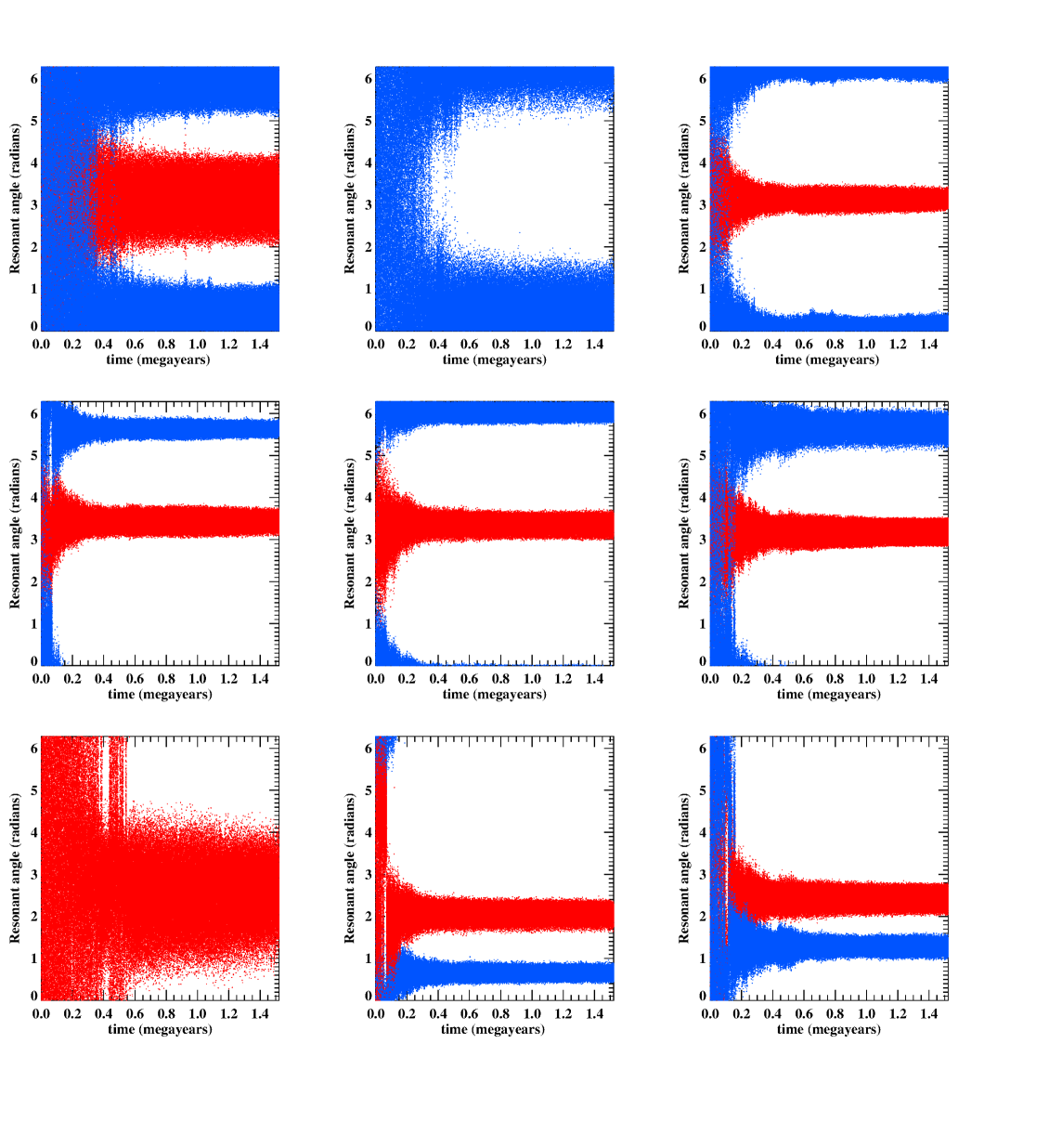
Figure 3: The evolution of the seven planet system with case A masses and $Q^{\prime}=100Q^{\prime}_{0}$ for all planets, resonant angles. The contents of the panels are as in Fig. 1.

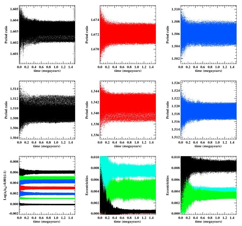
Figure 4: Results for the seven planet system with case A masses and $Q^{\prime}=100Q^{\prime}_{0}$ for all planets, period ratios and eccentricities. The contents of the panels are as in Fig. 2.

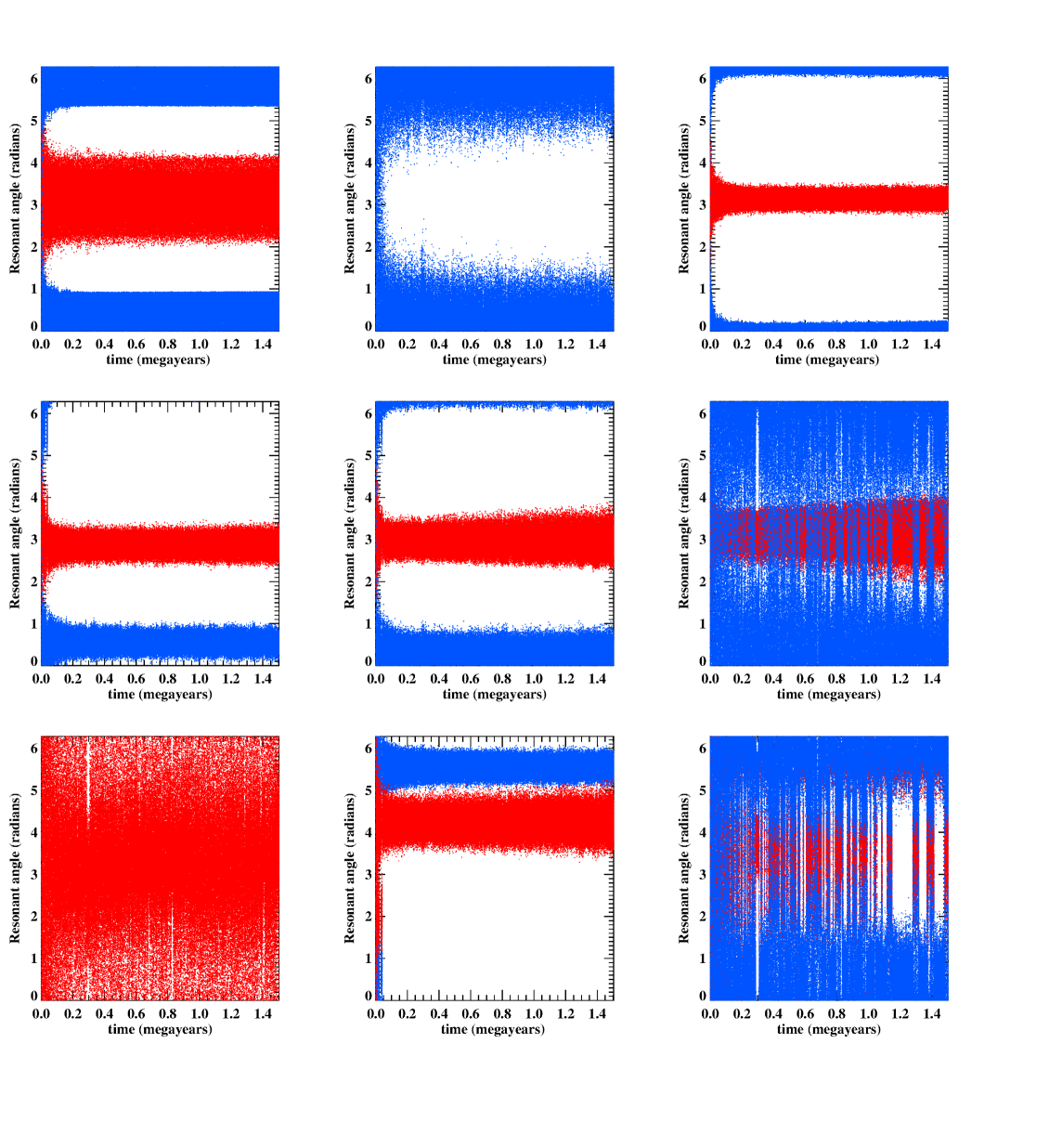
Figure 5: The evolution of the seven planet system with case B masses and $Q^{\prime}=Q^{\prime}_{0}$ for all planets, resonant angles. The contents of the panels are as in Fig. 1.

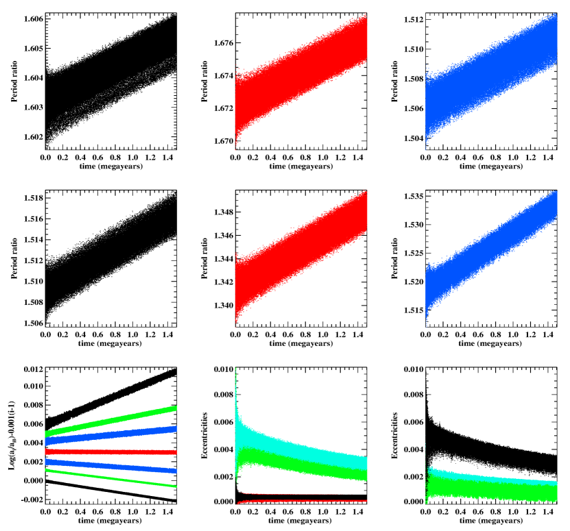
Figure 6: Results for the seven planet system with case B masses and $Q^{\prime}=Q^{\prime}_{0}$ for all planets, period ratios and eccentricities. The contents of the panels are as in Fig. 2.

Figure 7: The evolution of the seven planet system with case B masses and $Q^{\prime}=100Q^{\prime}_{0}$ for all planets, resonant angles. The contents of the panels are as in Fig. 1.

Figure 8: Results for the seven planet system with case B masses and $Q^{\prime}=100Q_{0}$ for all planets, period ratios and eccentricities. The contents of the panels are as in Fig. 2.

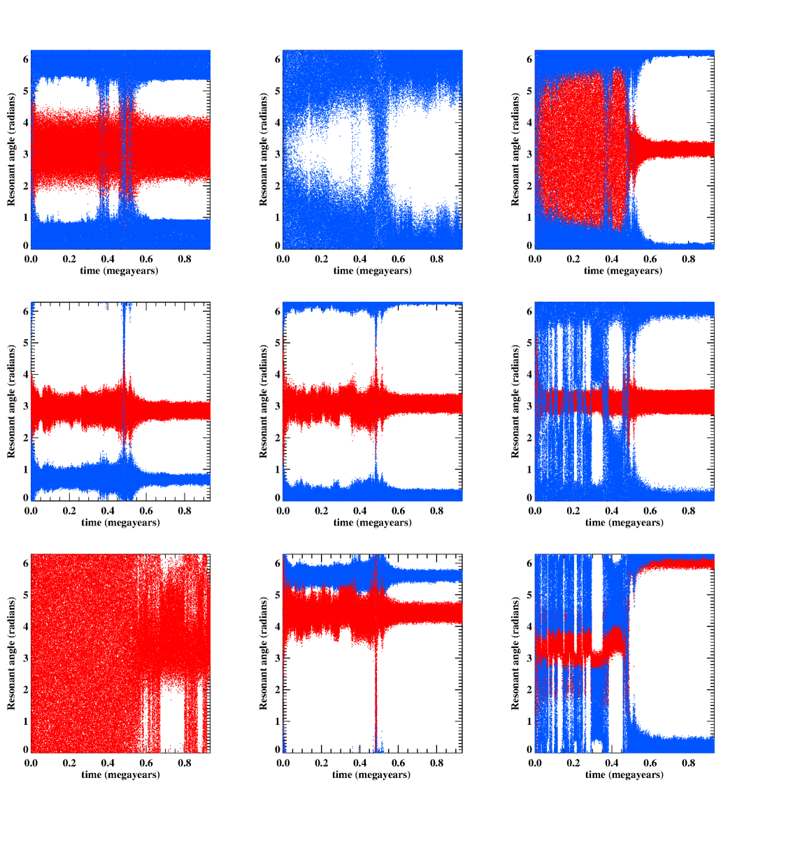
Figure 9: Results for $Q^{\prime}=Q^{\prime}_{0}$ but with inner three planets starting in a Laplace resonance with reduced semi-major axes, resonant angles. The contents of the panels are as in Fig. 1.

Figure 10: Results for $Q^{\prime}=Q^{\prime}_{0}$ but with inner three planets starting in a Laplace resonance with reduced semi-major axes, period ratios and eccentricities. The contents of the panels are as in Fig. 2.

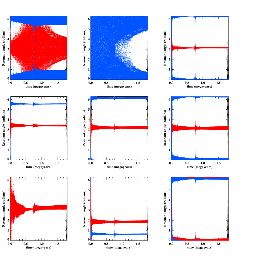
Figure 11: Results for $Q^{\prime}=Q^{\prime}_{0}$ and masses corresponding to model A and tides acting only on the inner two planets. Initial conditions are as for the run illustrated in Fig. 1 but with inner two planets starting in a closer 3:2 resonance with the outermost of the pair at a slightly reduced semi-major axis ,resonant angles. The contents of the panels are as in Fig. 1.

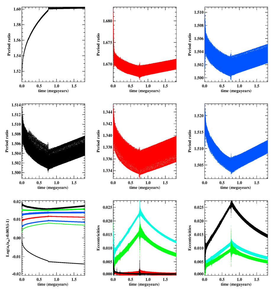
Figure 12: Results for $Q^{\prime}=Q^{\prime}_{0}$ and masses corresponding to model A and tides acting only on the inner two planets. Initial conditions are as for the run illustrated in Fig. 1 but with inner two planets starting in a closer 3:2 resonance with the outermost of the pair at a slightly reduced semi-major axis ,period ratios and eccentricities. The contents of the panels are as in Fig.2 apart from the lowermost left panel which shows $\log(a_{i}/a_{i0})-0.003(i-1)$ for $i=1-7,$ where $a_{i0}$ is the initial value of the semi-major axis of planet $i.$ Planets $1-7$ correspond to curves taking on monotonically increasing values ranging from lowermost to uppermost.

Figure 13: Evolution of the system in case A for $M_{d}=3.5\times 10^{-4}$ ${\rm M}_{\odot}$. The upper left plot shows $a$ versus time for the 6 planets and Q’=100. The upper right plot shows the ratio of the periods for pairs of planets versus time for Q’=100. Only the first $10^{5}$ years are shown, but the ratios stay almost constant after that time. The ratio $P_{5}/P_{4}$ is not shown but it stays constant equal to 1.5 for the whole duration of the simulation. The lower plots show $e$ versus time for the 6 planets and Q’=100 (left panel) and Q’=1000 (right panel).

Figure 14: Evolution of $\delta_{i,i+1}\equiv 100(P_{i+1}/P_{i}-r_{i,i+1})$, where $r_{i,i+1}$ is the initial ratio of the periods of planets $i$ and $i+1$. The upper panel corresponds to case A and $M_{d}=3.5\times 10^{-4}$ ${\rm M}_{\odot}$, $t_{\rm dis}=5\times 10^{5}$ years and $t_{\rm evol}=10^{5}$ years. The lower panel corresponds to case B and $M_{d}=3.5\times 10^{-4}$ ${\rm M}_{\odot}$, $t_{\rm dis}=4\times 10^{5}$ years and $t_{\rm evol}=10^{5}$ years. The value $\delta=1$ means a departure from exact commensurability of 1%. Note that the sharp increase of $\delta$ at the beginning of the simulations may be due to the initial set up, in which the resonant angles are not librating.

3 The expansion of multi-planet systems linked through a series of Laplace resonances driven by energy dissipation at fixed angular momentum

We here consider systems with consecutive planets linked by first order resonances and consecutive triples linked by Laplace resonances, though the latter may not apply in detail to all triples as in the TRAPPIST-1 system. We investigate how energy dissipation due to tidal circularization that acts on forced eccentricities but occurs while the total angular momentum of the system is conserved, leads to a secular expansion of the system with successive period ratios becoming increasingly disparate. We relate the rate of total energy dissipation to the rate of expansion when either all triples are linked by Laplace resonances, or when the system is composed of two subsystems each of which are fully linked by Laplace resonances. The evolution time scale for this process scales as $Q^{\prime}.$

In order to proceed we set the mean motion of planet $i$ to be $n_{i},$ it’s orbital period to be $P_{i}=2\pi/n_{i},$ it’s eccentricity to be $e_{i},$ the longitude of pericentre to be $\varpi_{i},$ and its longitude to be $\lambda_{i}.$ The systems we consider are such that consecutive planets are in first order resonances for which either one or two of the associated resonant angles librate. When both resonant angles librate for every pair, consecutive triples are linked through three body Laplace resonances ( see eg. Papaloizou 2015, 2016 ).

If planets, $i,$ and, $i+1,$ are in the first order $p_{i}:(p_{i}-1)$ resonance, with, $p_{i},$ being an integer that may be different for different pairs of planets, the relevant resonant angles are given by

$$\Phi_{i,i+1,1}=p_{i}\lambda_{i+1}-(p_{i}-1)\lambda_{i}-\varpi_{i},\hskip 8.53581pt{\rm and}$$

$$\Phi_{i,i+1,2}=p_{i}\lambda_{i+1}-(p_{i}-1)\lambda_{i}-\varpi_{i+i}.$$ (8)

$${\rm The\hskip 2.84526ptangle}\hskip 2.84526pt\Psi_{i+2,i+1,i}=\Phi_{i+1,i+2,1}-\Phi_{i,i+1,2}\hskip 2.84526pt$$

$${\rm which\hskip 2.84526ptcan\hskip 2.84526ptalso\hskip 2.84526ptbe\ \hskip 2.84526ptwritten}$$

$$\Psi_{i+2,i+1,i}=p_{i+1}\lambda_{i+2}-(p_{i}+p_{i+1}-1)\lambda_{i+1}+(p_{i}-1)\lambda_{i}$$

depends only on the longitudes and for it’s time derivative we have

$$\frac{d\Psi_{i+2,i+1,i}}{dt}=p_{i+1}n_{i+2}-(p_{i}+p_{i+1}-1)n_{i+1}+(p_{i}-1)n_{i}$$

$$+O\left(\frac{m_{i}e_{i}}{M}\right)$$ (9)

(see eg. Papaloizou 2015, 2016). Thus if the two associated first order resonant angles undergo small amplitude librations, given small eccentricities and mass ratios, this angle will also undergo small amplitude librations and the Laplace resonance condition

$$p_{i+1}n_{i+2}-(p_{i}+p_{i+1}-1)n_{i+1}+(p_{i}-1)n_{i}=0.$$ (10)

will hold. For large amplitude librations it will hold in a time average sense and we shall assume that the orbital elements we use in the simple modelling carried out below also correspond to appropriate time averages.

For a multi-planet system with $N>3$ members, there can be up to $N-2$ Laplace resonance conditions that hold, each one connecting three consecutive planets. When all of these apply, all but two of the semi-major axes are determined by the resonance conditions. When this occurs we exploit it by introducing the quantities

$$\Delta_{i}=n_{i}-n_{i+1},\hskip 8.53581pt{\rm for}\hskip 8.53581pti=1,2,..N-1.$$ (11)

Then

$$\frac{\Delta_{i+1}}{\Delta_{i}}=\frac{n_{i+1}-n_{i+2}}{n_{i}-n_{i+1}}=\frac{p_{i}-1}{p_{i+1}}$$ (12)

and we have

$$\Theta_{i,k}=\frac{\Delta_{i+k}}{\Delta_{i}}=\prod_{j=1}^{k}\frac{(p_{i+j-1}-1)}{p_{i+j}}\hskip 8.53581pt{\rm for}\hskip 8.53581ptk=1,2...N-i-1.$$ (13)

together with the specification $\Theta_{i,0}=1$.

Using (13) for $i=1,$ all of the mean motions in the system can be expressed in terms of $n_{1}$ and $\Delta_{1}.$ Thus

$$n_{i}-n_{i+k+1}=\Delta_{i}\sum_{j=0}^{k}\Theta_{i,j}$$ (14)

Differentiating (14) with respect to time we obtain

$$\frac{dE_{i+k+1}}{dt}-\left(\frac{m_{i+k+1}}{m_{i}}\right)\left(\frac{a_{i+k+1}}{a_{i}}\right)^{1/2}\frac{dE_{i}}{dt}=$$

$$\frac{m_{i+k+1}}{3}\sqrt{GMa_{i+k+1}}\frac{d\Delta_{i}}{dt}\sum_{j=0}^{k}\Theta_{i,j}$$

$${\rm for}\hskip 8.53581ptk=0,1,...N-i-1.$$ (15)

Writing this in terms of the angular momenta under the assumption that eccentricities are vanishingly small, we obtain

$$\frac{dJ_{i+k+1}}{dt}-\left(\frac{m_{i+k+1}}{m_{i}}\right)\left(\frac{a_{i+k+1}}{a_{i}}\right)^{2}\frac{dJ_{i}}{dt}=$$

$$\frac{m_{i+k+1}}{3}a_{i+k+1}^{2}\frac{d\Delta_{i}}{dt}\sum_{j=0}^{k}\Theta_{i,j}\hskip 4.2679pt{\rm for}\hskip 4.2679ptk=0,1,...N-i-1.$$ (16)

Setting $i=1$ in (15) and summing from $k=0$ to $k=N-2,$ we obtain

$$\frac{dE}{dt}-\alpha\frac{dE_{1}}{dt}=\sqrt{GM}\frac{d\Delta_{1}}{dt}\sum_{k=0}^{N-2}\left(\frac{m_{k+2}}{3}\sqrt{a_{k+2}}\sum_{j=0}^{k}\Theta_{1,j}\right),$$ (17)

where, $E,$ is the total energy of the system and

$$\alpha=\sum_{k=-1}^{N-2}\left(\frac{m_{k+2}}{m_{1}}\right)\sqrt{\frac{a_{k+2}}{a_{1}}}$$ (18)

Similarly (16) gives

$$\frac{dJ}{dt}-\beta\frac{dJ_{1}}{dt}=\frac{d\Delta_{1}}{dt}\sum_{k=0}^{N-2}\left(\frac{m_{k+2}}{3}a_{k+2}^{2}\sum_{j=0}^{k}\Theta_{1,j}\right),$$ (19)

where, $J,$ is the total angular momentum of the system and

$$\beta=\sum_{k=-1}^{N-2}\left(\frac{m_{k+2}}{m_{1}}\right)\left(\frac{a_{k+2}}{a_{1}}\right)^{2}.$$ (20)

Recalling the assumption that eccentricities are negligible, we can combine (17) and (19) so as to eliminate $dE_{1}/dt$ and $dJ_{1}/dt$ and thus obtain

$$\frac{dE}{dt}-\frac{n_{1}\alpha}{\beta}\frac{dJ}{dt}=$$

$$-\frac{1}{3}\frac{d\Delta_{1}}{dt}\sum_{k=0}^{N-2}m_{k+2}a_{k+2}^{2}\left(\frac{n_{1}\alpha}{\beta}-n_{k+2}\right)\sum_{j=0}^{k}\Theta_{1,j}.$$ (21)

For an isolated system the total angular momentum, $J,$ is conserved and we have

$$\frac{d\Delta_{1}}{dt}=-3\frac{dE}{dt}\left({\sum_{k=0}^{N-2}m_{k+2}a_{k+2}^{2}\left(\frac{n_{1}\alpha}{\beta}-n_{k+2}\right)\sum_{j=0}^{k}\Theta_{1,j}}\right)^{-1}.$$ (22)

Thus the rate of expansion of the system, which can be shown to be positive definite, is directly proportional to the rate of energy dissipation, here associated with tidal circularization and is thus $\propto 1/Q^{\prime}$. In a system linked together with consecutive three body Laplace resonances, the mean motion separation between any two planets is $\propto\Delta_{1},$ (see (14)). For tidal circularization the rate of energy dissipation associated with a particular planet is proportional to the square of the eccentricity, which is $\propto 1/\Delta_{1}^{2}$ (e.g. Papaloizou 2011). Hence $dE/dt=(dE/dt)_{0}(\Delta_{1,0}/\Delta_{1})^{2},$ where $\Delta_{1,0}$ is the value of $\Delta_{1}$ at time $t=t_{0}$ and $(dE/dt)_{0}$ is the value of $dE/dt$ at that time. Integrating (22) with respect to time assuming that quantities other than the $\Delta_{i}$ may assumed to be constant, we obtain

$$\Delta_{1}^{3}-\Delta_{1,0}^{3}=-9(t-t_{0})\Delta_{1,0}^{2}$$

$$\times\left(\frac{dE}{dt}\right)_{0}\left({\sum_{k=0}^{N-2}m_{k+2}a_{k+2}^{2}\left(\frac{n_{1}\alpha}{\beta}-n_{k+2}\right)\sum_{j=0}^{k}\Theta_{1,j}}\right)^{-1}$$ (23)

Hence for a system of arbitrary numbers of planets linked by consecutive Laplace resonances such that the separations of neighbouring mean motions are all proportional to each other, asymptotically $\Delta_{1}\propto t^{1/3}$ as has been found in other contexts where tidal dissipation operates (e.g. Papaloizou 2011, 2015).

3.1 Systems composed of two subsystems

The TRAPPIST-1 system is such that a Laplace resonance condition connected to the existence of two first order resonances does not apply to planets c , d and e. However, it does potentially apply to all other consecutive triples. Thus the system can be regarded as a composite one in which planets b, c and d form an inner subsystem with such a Laplace resonance while planets d - h form an outer subsystem linked by such Laplace resonances.

In the appendix we repeat the analysis for a system composed of two such subsystems with planets, $1,2,...N_{1},$ forming an inner subsystem and planets, $N_{1}+1,N_{1}+2,...N,$ forming an outer subsystem. For the TRAPPIST-1 system $N_{1}=3.$ For such a system it is found that (21) is replaced by the equation

$$\frac{dE}{dt}-\frac{n_{1}\alpha}{\beta}\frac{dJ}{dt}=\frac{d\Delta_{1}}{dt}\left(\sum_{k=0}^{N-2}\frac{m_{k+2}a_{k+2}^{2}}{3}\left(n_{k+2}-\frac{n_{1}\alpha}{\beta}\right)\Lambda_{k}\right)$$ (24)

where

$$\Lambda_{k}=\frac{n_{1}-n_{k+2}}{n_{1}-n_{2}}\hskip 8.53581pt{\rm for}\hskip 8.53581ptk<N_{1}-1,\hskip 8.53581pt{\rm and}$$ (25)

$$\Lambda_{k}=\frac{n_{N_{1}}-n_{k+2}}{n_{N_{1}}--n_{N_{1}+1}}\frac{d\Delta_{N_{1}}}{d\Delta_{1}}+\frac{n_{1}-n_{N_{1}}}{n_{1}-n_{2}}\hskip 8.53581pt{\rm for}\hskip 8.53581ptk\geq N_{1}-1.$$ (26)

We remark that when $\Delta_{N_{1}}$ and $\Delta_{1}$ increase monotonically with time, as found for the cases we have simulated, $\Lambda_{k}$ is easily shown to be positive definite and an increasing function of $k.$ This is sufficient to ensure that the quantity multiplying $d\Delta_{1}/dt$ in (24) is negative. It then follows that if the total angular momentum of the system is conserved, energy dissipation drives its progressive expansion.

When $\Delta_{N_{1}}/\Delta_{1}$ is constant corresponding to the situation where the ratio $(n_{i}-n_{i+1})/(n_{j}-n_{j+1})$ being independent of time for $1<i<N-1,$ $1<j<N-1,$ equation (24) takes the same form as (21) when $\Theta_{1,j}$ is expressed in terms of the mean motions. For more general cases, as long as both $\Delta_{1},$ and $\Delta_{N_{1}}$ increase with time, the quantity in brackets is always positive so that we conclude that energy dissipation drives the expansion just as before and (23) will hold with the quantity $\sum_{j=0}^{k}\Theta_{1,j}$ replaced by an appropriate mean value of $\Lambda_{k}.$

4 Numerical Simulations

In this section we present the results of numerical simulations of the TRAPPIST-1 system that incorporate tidal circularization. Thus the initial conditions in most cases were taken to correspond to the tabulated orbital elements given by Gillon et al. (2017) and Luger et al. (2017) The eccentricities were assumed to be zero. We remark that the actual eccentricities cannot be strictly zero with the consequence that we start with a system that will not have an exact correspondence to the actual one but will be only close to it. However, the simulations incorporate dissipative effects which cause the system to approach a well defined evolutionary state, a feature that may mitigate the effects of not starting with initial conditions which exactly correspond to the observed system.

We consider two sets of masses corresponding to models A and B respectively. The parameters adopted for models A and B are listed in table 1. Apart from the outermost planet’s mass, those for model A were taken from Gillon et al. (2017) and Luger et al. (2017). A value for the outermost mass is not available so we have simply estimated it by assuming a mean density corresponding to the earth. Those for model B were taken from Wang et al. (2017) who quote a significantly smaller value for the outermost mass. We note that the error bars are large and we have retained the model A masses of the inner four planets in model B as differences are within them. We remark that the planetary radii are the same for models A and B. We comment that tests have shown that inclusion of the outermost planet does not affect the general form of the results for the remaining planets. The simulations were by means of $N$–body calculations (see eg. Papaloizou & Terquem 2001). From considerations of numerical tractability we are unable to consider very large values of $Q^{\prime}$ and very long integration times. Values of $Q^{\prime}$ up to $\sim 12$ and integration times up to $\sim 1.5\times 10^{6}y$ have been considered.

4.1 Numerical Results

Planet	Mass	Mean density	Mass	Mean density	Period	Period ratio
–	$m/M_{\oplus}$	${\overline{\rho}}/{{\overline{\rho}}_{\oplus}}$	$m/M_{\oplus}$	${\overline{\rho}}/{{\overline{\rho}}_{\oplus}}$	$P$	$P_{i}/P_{i-1}$
–	model A	model A	model B	model B	–	–	–
1(b)	0.85	0.66	0.85	0.66	1.51087081	–
2(c)	1.38	1.17	1.38	1.17	2.4218233	1.602932087
3(d)	0.41	0.89	0.41	0.89	4.049610	1.672132727
4(e)	0.62	0.80	0.62	0.80	6.099615	1.506222821
5(f)	0.68	0.6	0.36	0.32	9.206690	1.509388707
6(g)	1.34	0.94	0.57	0.40	12.35294	1.341735195
7(h)	0.37	1.0	0.086	0.23	18.764	1.518990621

Table 1: The masses, mean densities and orbital periods in days for the planetary systems simulated here. The masses and mean densities for model A were obtained from Gillon et al. (2017) and Luger et al. (2017) and those for model B from Wang et al. (2017) (see the text for more details). We remark that the planetary radii adopted in both cases are the same. The final column contains the period ratio with the next innermost planet where applicable.

We begin by describing the results for the model A system with, apart from the eccentricities being set to zero, initial conditions from Gillon et al. (2017) and Luger et al. (2017) and with $Q^{\prime}=Q^{\prime}_{0}=0.122127.$ For this value of $Q^{\prime},$ the evolution of the period ratios in the system could be clearly exhibited on a $10^{6}y$ time scale. For this particular simulation circularization tides were applied only to the inner two planets. It was found that outcomes are virtually the same when tides are applied to all of the planets consistent with a rapid decrease of the effectiveness of tides with increasing semi-major axis. In addition, dynamical communication between the planets is effective enough to enable libration states to be attained for the outer planets through dissipative processes acting on the inner ones. The value of $Q^{\prime}$ adopted is unrealistically small. However, apart from slower evolution rates, the same characteristic behaviour is found for values of $Q^{\prime}$ up to $100Q^{\prime}_{0}.$ The evolution of the resonant angles is shown in Fig.1. These exhibit a behaviour that is characteristic of all of the simulations starting with initial conditions close to those given for the present system.

The uppermost left panel of Fig. 1 shows the behaviour of the resonant angles $3\lambda_{2}-2\lambda_{1}-\varpi_{2}$ and $3\lambda_{2}-2\lambda_{1}-\varpi_{1}$ that connect the innermost pair of planets. Although not in a state of libration initially these angles both rapidly attain such a state with the libration of the former being about $\pi$ and the latter about zero. The amplitudes are quite large. A similar behaviour is found for the resonant angle $3\lambda_{3}-2\lambda_{2}-\varpi_{2}$ connecting planets $2$ and $3$ which ultimately librates about zero and is illustrated in the uppermost middle panel. On the other hand the angle $3\lambda_{3}-2\lambda_{2}-\varpi_{3}$ does not attain libration. This evolution results in a Laplace resonance being set up for planets $1,2,$ and $3,$ but a corresponding one cannot be set up for planets $2,3,$ and $4$ (see the discussion at the beginning of Section 3).

The resonant angles $3\lambda_{4}-2\lambda_{3}-\varpi_{4}$ and $3\lambda_{4}-2\lambda_{3}-\varpi_{3}$ which connect planets $3$ and $4$ illustrated in the uppermost right panel also rapidly attain a librating state analogous to those connecting $1$ and $2,$ the former librating about $\pi$ and the latter about zero, but with smaller libration amplitudes. A corresponding behaviour for the resonant angles $4\lambda_{6}-3\lambda_{5}-\varpi_{6}$ and $4\lambda_{6}-3\lambda_{5}-\varpi_{5}$ connecting planets $5$ and $6$ is illustrated in the middle panel of the central row. This is also found for the resonant angles $3\lambda_{7}-2\lambda_{6}-\varpi_{7}$ and $3\lambda_{7}-2\lambda_{6}-\varpi_{6}$ illustrated in the right panel of the middle row.

The resonant angles $3\lambda_{5}-2\lambda_{4}-\varpi_{5}$ and $3\lambda_{5}-2\lambda_{4}-\varpi_{4}$ that connect planets $4$ and $5$ illustrated in the left panel of the middle row also librate but while the former librates about $\pi,$ the latter librates about an angle $\sim\pi/4.$ This may be connected to the fact that there are first order resonances connecting non consecutive planets. In particular there are 2:1 resonances connecting planets $4$ and $6$ and also $5$ and $7.$ The lowermost middle panel of Fig.1 shows the resonant angles $2\lambda_{6}-\lambda_{4}-\varpi_{6}$ and $2\lambda_{6}-2\lambda_{4}-\varpi_{4}$ and the lowermost right panel shows the resonant angles $2\lambda_{7}-\lambda_{5}-\varpi_{7}$ and $2\lambda_{7}-2\lambda_{5}-\varpi_{5}$. In the former case the libration centres are not zero or $\pi$ while in the latter both are close to zero. The behaviour of these angles is consistent with all triples being connected with a Laplace resonance with related first order resonances except $2,$ $3$ and $4.$ Thus in the notation of Section 3 where subsystems are discussed, the inner three planets can be viewed as forming an inner subsystem with, $N_{1}=3,$ while the remaining planets form a separate outer subsystem.

In addition to librating in a first order 3:2 resonance, though quite distant from precise commensurability, planets $2$ and $3$ are also close to a 5:3 resonance, though being second order this may not be expected to play a significant role on account of the small eccentricities. However, the resonant angle $5\lambda_{3}-2\lambda_{2}-\varpi_{3}$ illustrated in lowermost left panel of Fig. 1 indicates periods of large amplitude libration indicating that this resonance may be involved in the dynamics.

The time evolution of the period ratios of consecutive planets and orbital eccentricities is shown in Fig. 2. The period ratios $P_{2}/P_{1},$ $P_{3}/P_{2},$ $P_{4}/P_{3},$ $P_{5}/P_{4},$ $P_{6}/P_{5}$ and $P_{7}/P_{6}$ all tend to increase with time in the same way. This is consistent with the expansion of the system discussed in Section 3 where it is argued that the evolution time scales as $Q^{\prime}.$ For the simulation discussed here with $Q^{\prime}=Q^{\prime}_{0}$, period ratios depart significantly from initial values after $\sim 2\times 10^{6}y,$ indicating values of $Q^{\prime}$ in the range $10^{2-3}$ are required if the system is to remain near the present state over $Gy$ time scales. The evolution of the semi-major axes of all of the planets is illustrated in the lowermost left panel. We plot $\log(a_{i}/a_{i0})-0.001(i-1)$ for $i=1-7,$ where $a_{i0}$ is the initial value of the semi-major axis of planet $i.$ The shift $-0.001(i-1)$ is applied simply to allow visibility of all curves. The innermost four planets migrate inwards and the outermost three outwards as consistent with a general expansion of the whole system while conserving total angular momentum as described in Section 3. In addition planet $3$ migrates inwards such that both $\Delta_{N_{1}}$ as well as $\Delta_{1}$ increase with time as assumed in Section 3. The eccentricities of all the planets are illustrated in the lowermost middle and right panels. While remaining small and $<0.01,$ they decrease secularly with time. This is a consequence of the increasing period ratios which move planet pairs further away from resonance.

4.2 Dependence on $Q^{\prime}$

In order to investigate the dependence on, $Q^{\prime},$ we present the results of a simulation with the same parameters as the preceding one except that $Q^{\prime}=100Q^{\prime}_{0}$ but with tides now allowed to act on all of the planets. The evolution of the resonant angles is shown in Fig. 3. This plots the same quantities that are shown in Fig. 1 for the case with $Q^{\prime}=Q^{\prime}_{0},$ so that the results may be directly compared. We see that the resonant angles connecting planets $1$ and $2,$ those connecting planets $2$ and $3,$ those connecting $3$ and $4,$ those connecting $5$ and $6$ and those connecting $6$ and $7,$ apart from taking longer to establish clear libration, show very similar behaviour. The increase in the time required to establish libration can be up to two orders of magnitude but is not uniform and the libration amplitudes are somewhat larger. The resonant angles $3\lambda_{5}-2\lambda_{4}-\varpi_{5}$ and $3\lambda_{5}-2\lambda_{4}-\varpi_{4}$ that connect planets $4$ and $5$ illustrated in the left panel of the middle row librate as before but with the latter now librating about an angle $\sim 7\pi/4.$ The resonant angles associated with the $2:1$ resonances connecting non consecutive planets shown in the lowermost panels also show shifts of libration centre as compared to the previous simulation.

The behaviour of the period ratios and eccentricities is illustrated in Fig. 4 and it can be directly compared to that for the previous simulation illustrated in Fig. 2. It will be seen that with the much larger $Q^{\prime},$ the period ratios do not show a noticeable secular increase and the system as a whole does not show a measurable expansion. This is because the eccentricity damping time scale is increased by a factor of a hundred in this case resulting in a corresponding increase in the evolution time scale for the period ratios which accordingly do not show significant evolution over the time shown here. However, it is possible to detect period ratio evolution for values of $Q^{\prime}$ up to $10Q^{\prime}_{0}$ over this time period. Simulations with $Q^{\prime}=Q^{\prime}_{0}$ and $Q^{\prime}=10Q^{\prime}_{0}$ were used to verify that the rate of period ratio evolution was indeed $\propto 1/Q^{\prime}$ as expected from the discussion of Section 3.

4.3 Effect of changing the masses

To investigate the effect of changing the masses we present the results of two simulations with the same parameters as the preceding two, except that masses corresponding to model B were adopted and tides were applied to all planets. The evolution of the resonant angles for the case $Q^{\prime}=Q^{\prime}_{0}$ is illustrated in Fig. 5 and for the case $Q^{\prime}=100Q^{\prime}_{0}$ is illustrated in Fig. 7. The period ratios and eccentricities for these simulations are shown in Figs. 6 and 8 respectively. A comparison with the preceding simulations for which masses appropriate to model A were used indicates similar behaviour for the resonant angles. However, libration amplitudes are larger and it can take longer to attain librating states. This is particularly the case for angles associated with the outermost planet which seems in general to show less stable behaviour on account of its low mass. The behaviour of the period ratios and eccentricities is similar to the case for which the masses were appropriate to model A. The evolution of the semi-major axes in the case with $Q^{\prime}=Q^{\prime}_{0}$ is such that the inner three planets migrate inwards, for the fourth planet it remains on average nearly constant, while the outer three move outwards. On account of its small mass, the outermost planet moves outwards significantly more rapidly than the simulation with case A masses and $Q^{\prime}=Q^{\prime}_{0}.$

4.4 Interaction of the inner and outer subsystems

Apart from planets 2 and 3, consecutive pairs of planets in the TRAPPIST-1 system are linked by first order resonances for which both associated angles librate and are configured such that Laplace resonance conditions connecting consecutive triples may hold in a time average sense for every case except planets $2,$ $3$ and $4.$ Furthermore the deviations from exact commensurability are much greater for the innermost three. This indicates that the system may be viewed as being comprised of two subsystems of the type considered in Section 3 that are completely linked by such Laplace resonances. The innermost one consisting of the first three planets and the outermost one of the remainder.

In this section we provide a preliminary exploration of the possibility that a subsystem consisting of either the inner two or three planets formed separately from the rest and subsequently interacted with them. In particular we suppose that the inner subsystem expanded to interact with the outer subsystem that was essentially stationary, though we remark that there are variations of this such as where the outer subsystem migrates inwards while the inner one remains stationary that are likely to lead to similar conclusions. To explore this scenario, we present the results of simulations for which either the system was set up with the inner three planets in a Laplace resonances but with smaller initial semi-major axes, or for which only the inner two planets were similarly set up in a closer 3:2 resonance. The separate subsystems then expand with much weakened coupling to the corresponding outer system. Parameters are set such that the systems begin to interact more strongly when conditions corresponding to the current observed system are approached and we investigate whether the interaction leads to the system eventually evolving in a similar way to the one initiated with initial conditions corresponding to the observed system.

We do not consider the history of the outer system, noting that it could be in a different configuration to that corresponding to the same planets in the observed system. For example if it migrated inwards until reaching a protoplanetary disc edge that was progressively moving outwards, allowing the inner system that formed earlier to have moved closer to the star, the resonances might have been closer to commensurability.

In the first simulation presented in this Section, tidal circularization is applied only to the innermost two planets, with $Q^{\prime}=Q^{\prime}_{0},$ and the masses corresponded to model A. The system was set up as for the observed system with the difference that the initial periods of planets $1$, $2$ and $3$ were set to $1.52647745$ days, $2.422519714$ days and $3.97777737$ days respectively. As in all other cases the initial eccentricities were set to zero. These correspond to the period ratios $P_{2}/P_{1}=1.587,$ and $P_{3}/P_{2}=1.642.$ These are smaller than for the observed system as they correspond to a situation where the inner subsystem of planets $1$, $2$ and $3$ is in a Laplace resonance but is less expanded. Note that although planet $3$ is at a reduced period as compared to the observed system, planet $1$ has a longer period. The evolution of the resonant angles for this simulation is illustrated in Fig. 9. and the evolution of the period ratios is illustrated in Fig. 10.

The evolution can be split into two phases. Before the subsystems start to interact significantly at time $\sim 4.5\times 10^{5}y,$ the inner system evolves like a separate system of $N=3$ planets linked by a Laplace resonance as described in Section 3 and equations (22) and (23) apply (see also Papaloizou 2015). From Fig. 10, the estimated time for this subsystem to separate to attain current period ratios starting from 3:2 commensurabilites is $\sim 10^{6}y,$ again indicating that values of $Q^{\prime}\sim 10^{2-3}$ are needed in order to obtain evolution on $Gy$ time scales.

During the first phase the outer planetary system is only weakly coupled to the inner one. Thus the associated resonant angles show more erratic behaviour than the observed system though many show libration while the outer period ratios do not show a secular increase. After an initial interaction phase is complete at $t\sim 6\times 10^{5}y$ the entire system enters an evolutionary phase resembling that obtained when one starts with parameters corresponding to the observed system with resonant angles showing stable librations and the period ratios secularly increasing. In order to investigate the behaviour of orbits with initial conditions in the neighbourhood of those implemented above we considered additional simulations for which the orbital phases of all planets were randomised. Out of fourteen such realisations, four evolved in the same way as described above, the Laplace resonance being broken in the other cases with subsequent evolution causing the period ratio, $P_{3}/P_{2}$ to decrease and thus move away from the value appropriate to the observed system. This indicates that in spite of some fragility, the form of evolution that approaches that found for initial parameters corresponding to the observed system is not that of an isolated case.

In the second simulation presented in this Section, the set up was as for the observed system except that the initial periods of the inner two planets were taken to be $1.60239588$ days and $2.414794275$ days. Other parameters were the same as those for the the first simulation described in this Section. This corresponds to an initial period ratio of $1.5069$ for the innermost pair while planets $2$ and $3$ are slightly more separated than in the observed system with a period ratio of $1.677.$ Thus the inner pair starts in a close 3:2 resonance with the second planet just wide of a 5:3 resonance with the third. In this case the inner pair, assumed to have formed separately, a possibility indicated in Section 5.1 below, separates as a result of tidal interaction and thus interacts with the outer planets.

The evolution of the resonant angles for this simulation is illustrated in Fig. 11 and the evolution of the period ratios is illustrated in Fig. 12. As the inner two planets separate, the period ratio between the second and third planets decreases and a 5:3 resonance is formed. This couples them to the outer planets transferring angular momentum to them and increasing their eccentricities. The latter phenomenon results in decreasing period ratios, just as decreasing eccentricities leads to them increasing. After about one megayear the period ratio of the innermost pair has increased enough to enable the inner three planets to settle into a Laplace resonance, when the required condition on the mean motions is satisfied. Subsequently the evolution approaches that of the observed system for which the eccentricities decrease and the period ratios increase secularly with time.

To establish that orbits close in phase space to the one illustrated above undergo the same type of evolution, we interrupted it at a late stage but well before attaining the final state corresponding to the observed system and randomised the orbital phases of all planets for ten different realisations. This caused the 5:3 resonance between planets 2 and 3 to be broken. However after a brief relaxation phase it was reestablished and their evolution approach the same form as in the uninterrupted case.

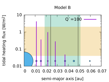
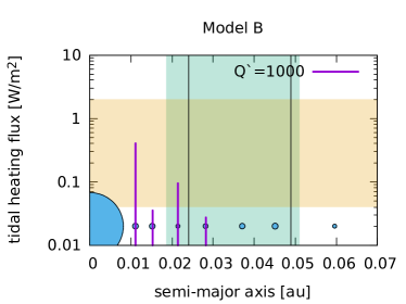
Figure 15: The TRAPPIST-1 system together with its habitable zones (insolation zone in green and tidal zone in yellow). The violet impulses show the amount of the tidal heating flux produced by each planet. The tidal heating flux in the range from 0.04 till 2 $W/m^{2}$ favours plate tectonics. The results are shown for two different sets of planets’ masses: model A (left) and model B (right) and for two different values of $Q^{\prime}$: 100 (upper panels) and 1000 (lower panel). The borders of the conservative habitable zone are marked by two vertical black lines.

5 Maintenance of commensurabilities when a protoplanetary disc is present and the effect of disc dispersal on resonant chains

Tamayo et al. (2017) have suggested that the chain of resonances in the TRAPPIST-1 system may have formed while the planets were migrating through the disc towards the central star. In their simulations, all the planets are subject to eccentricity damping due to interaction with the disc, but only the outermost planet 7 feels a direct migration force at the beginning of the calculation. After it captures planet 6 into a resonance, the pair migrates in together, which leads to capture of planet 5 and so on, until all the planets are in resonances. It is found that by adjusting the ratio of the migration and eccentricity damping timescales the observed chain of commensurabilities can be reproduced. However, an issue with this is that all the planets should be subject to direct migration forces from the beginning of the calculation. The interaction with the disc that leads to eccentricity damping also in general produces migration torques unless there is a balance between Lindblad and corotation torques for each planet apart from the outermost one. It would seem unlikely that this could be maintained at all disc locations that they move through. The migration prescription is not an arbitrary function but should be related to a disc and have an appropriate dependence on the planet mass (see eg. Papaloizou 2016).

As shown below, planet 2 is expected to migrate faster than planet 3 because, being significantly more massive, it interacts more strongly with the disc. As a consequence, it cannot maintain a resonance with planet 3 while the system migrates through the disc. Therefore planets 1 and 2 reach the disc inner parts before the other planets, and the chain of resonances can be established only after all the planets have arrived in the central parts and terminate migration there. Termination may be due either to the planets entering an inner cavity, or to the innermost planet stalling just beyond the disc’s inner edge.

Masset et al. (2006) have indeed suggested that cores could be trapped at the edge of the disc, rather than penetrating inside the cavity, through the operation of corotation torques. Whether that happens or not is not clear, as it may depend on the level of MHD turbulence at the inner edge. Also, if the disc’s inner edge moves out because of X–ray photo-evaporation, the surface density of gas in the vicinity of the innermost planet would decrease to zero. In that case, the disc cannot transfer enough angular momentum to the planet for it to stay coupled and move outward with the retreating inner edge. Given the uncertainties, here we consider both possibilities, with either the planets entering the cavity, or stalling just beyond the disc’s inner edge.

Ormel, Liu and Schoonenberg (2017) have considered a model in which the planets in the TRAPPIST-1 system move inward and stall at the disc’s inner edge. They assume that consecutive pairs among planets 1 to 5 are initially in 3:2 MMRs, and they investigate the conditions under which these can be broken for the two innermost pairs, which are observed to be close to 8:5 and 5:3 commensurabilities. Ormel et al. (2017) assume that the disc’s inner edge moves out due to the expansion of the magnetospheric cavity, and that the planets decouple from the disc one after the other, starting with the innermost one. As decoupling happens on a timescale which depends on the planet’s mass, a period of divergent migration may take place when a planet has decoupled and the next outermost one is temporarily moving outward with the disc. By adjusting the expansion rate of the disc’s inner edge, Ormel et al. (2017) have found that the MMRs for the two innermost pairs could be broken. It is not clear however how these planets would then attain the observed period ratios that are consistent with there being a three body Laplace resonance between the inner three planets as indicated in our discussion in Sections 3, 4.1 and 4.4.

Note that in Section 3 we have presented an alternative scenario where the large separations from strict 3:2 commensurabilities for the two innermost pairs can in fact be produced through tidal interaction with the central star.

In this section, we consider a system of 6 planets which start close to the disc’s inner edge and which either subsequently enter an inner cavity, or stall just beyond the disc’s inner edge in a resonant chain. We ignore the outermost planet as its mass is not well constrained, but this does not affect the conclusions of our study. The goal of these simulations is to study whether commensurabilities can be maintained during the evolution of the system and the disc.

5.1 Planetary systems that enter the cavity

We set up the 6 inner planets of the TRAPPIST-1 system on circular orbits in a disc with inner edge at $r\equiv R_{\rm in}=0.05$ AU. The value of $R_{\rm in}$ is chosen so that the innermost planet is close to its current location after all the planets have penetrated inside the cavity. The orbit of the innermost planet is set with a semi-major axis $a_{1}=0.055$ AU. We consider two different sets of initial conditions, where planets 2 to 6 are started at distances such that $P_{2}/P_{1}=8/5$, $P_{3}/P_{2}=5/3$ (case A) or $P_{2}/P_{1}=3/2$, $P_{3}/P_{2}=3/2$ (case B) while $P_{4}/P_{3}=P_{5}/P_{4}=3/2$ and $P_{6}/P_{5}=4/3$ in both cases. Case A is close to the observed system. The motivation for considering case B is that this configuration would be easier to obtain through migration as it involves only first order resonance, and the configuration of the final chain of MMRs may have resulted from later tidal interaction with the star (see, e.g., Section 4.4). We then solve the equations of motion (1) for each planet where accelerations due to tidal interaction with the disc are given by equations (3) and (4). In the regime of inward type–I migration, Papaloizou & Larwood (2000) have shown that the migration and eccentricity damping timescales can be written as:

$$\begin{split}t_{mig,i}=146.0\;\left[1+\left(\frac{e_{i}}{1.3H/r}\right)^{5}\right]\left[1-\left(\frac{e_{i}}{1.1H/r}\right)^{4}\right]^{-1}\\ \left(\frac{H/r}{0.05}\right)^{2}\;\frac{{\rm M}_{\odot}}{M_{d}}\;\frac{{\rm M}_{\oplus}}{m_{i}}\;\frac{a_{i}}{{\rm 1~{}au}}\left(\frac{{\rm M}_{\odot}}{M}\right)^{1/2}\;\;\;{\rm years},\end{split}$$ (27)

and

$$\begin{split}t_{e,i}^{d}=0.362\;\left[1+0.25\left(\frac{e_{i}}{H/r}\right)^{3}\right]\;\left(\frac{H/r}{0.05}\right)^{4}\\ \frac{{\rm M}_{\odot}}{M_{d}}\;\frac{{\rm M}_{\oplus}}{m_{i}}\;\frac{a_{i}}{{\rm 1~{}au}}\left(\frac{{\rm M}_{\odot}}{M}\right)^{1/2}\;\;\;{\rm years},\end{split}$$ (28)

Here $H/r$ is the disk aspect ratio, which is taken to be 0.05, and $M_{d}$ is the disk mass contained within 5 au. The equations assume that the disc surface mass density $\propto r^{-3/2}$. The eccentricity damping timescale taking into account both tidal interaction with the star and disc interactions can be calculated through $1/t_{e,i}=1/t_{e,i}^{d}+1/t_{e,i}^{s}$, where $t_{e,i}^{s}$ is given by equation (6).

Masses derived for the $\sim$ 1 Myr old discs in the Ophiuchus star-forming region are on the order of 0.01 ${\rm M}_{\odot}$ within 50 AU (Andrews et al. 2010). Most of the stars in this study have a mass between 0.6 and 2 ${\rm M}_{\odot}$. As these discs are best fitted with a surface mass density $\propto r^{-1}$, this implies that the mass within 5 AU is on the order of $10^{-3}$ ${\rm M}_{\odot}$ after 1 Myr. In addition, observations and modelling of discs around T Tauri stars in the Taurus and Chamaelon I molecular cloud complex suggest that the disc’s mass decreases by a factor 10 during the first Myr of evolution (Hartmann et al. 1998). If we assume that the disc mass scales with the central mass, this suggests that the mass within 5 AU in the disc surrounding TRAPPIST-1 would have been roughly between $10^{-4}$ and $10^{-3}$ ${\rm M}_{\odot}$ during the first Myr of evolution.

Figure 13 shows the evolution of the system for case A and $M_{d}=3.5\times 10^{-4}$ ${\rm M}_{\odot}$. Both $Q^{\prime}=100$ and $Q^{\prime}=1000$ are considered. The evolution of the semi-major axes and period ratios are only shown for $Q^{\prime}=100$, but the plots for $Q^{\prime}=1000$ are very similar. As the planets migrate inward, they get closer to each other so that the eccentricities increase. They subsequently decrease in the case $Q^{\prime}=100$ when the innermost planet reaches radii small enough that tidal interaction with the star becomes important. Note that similar eccentricities are obtained when the mass of the disc is halved. The 3:2 and 4:3 MMRs between planets 4 and 5 and between planets 5 and 6, respectively, that were present initially, are maintained during the whole duration of the simulation. Planets 2 and 3 were initially in a 5:3 MMR, but as planet 2 is significantly more massive it migrates faster than planet 3 and the MMR is destroyed. Only after planet 2 penetrates into the cavity can planet 3 catch up and at that point a 2:1 MMR is established. In addition planets 1 and 2 establish a 3:2 resonance that is maintained for the duration of the simulation. Planets 3 and 4 were initially in a 3:2 MMR, but this gets temporarily destroyed as planet 3 is dragged behind planet 2 at the beginning of the simulation. After some time though, the 3:2 MMR is re–established. After the phase of readjustment of the MMRs, all the resonant angles and/or angles between the apsidal lines for pairs of consecutive planets librate around some fixed value, and departure from exact commensurability is at most of a few tenths of a percent.

Similar results are obtained in case B, except that planets 1 and 2, initially set up in a 3:2 MMR, remain in this resonance for the whole duration of the simulation. In this case again, planets 2 and 3 end up in a 2:1 MMR, even though they started in a 3:2 MMR.

The calculations described here show that the observed chain of MMRs cannot be established as planets migrate through the disc because planet 2 migrates too fast for a resonance with planet 3 to be maintained. This indicates that planets 1 and 2 must have reached the disc’s inner parts before the rest of the system, and MMRs were later established when the outer planets joined them. If planets have indeed been able to penetrate inside a cavity, rather than stall beyond the disc’s inner edge, large eccentricities must have been excited during the migration process. As the upper limit on the observed eccentricities is of a few percent, stellar tides must have been efficient enough to damp the eccentricities produced by the migration process.

5.2 Planets stalled beyond the disc’s inner edge

We now study the evolution of the system when the planets stall beyond the disc’s inner edge. We set up the 6 planets on circular orbits at the distance from the star where they are currently observed, and with consecutive planets in MMRs. Here again we consider both cases A and B. We assume that the disc’s inner edge lies just interior to the location of the innermost orbit. The tidal torque from this edge prevents the innermost planet from migrating inside the cavity. This torque is passed on from one planet to the next, and as a result all the planets are prevented from migrating inwards. However, as they are still embedded in the disc they are still subject to eccentricity damping. We therefore adopt the same governing equations as in the previous Section with the same eccentricity damping timescale, $t_{e,i}^{d},$ but ignoring $t_{mig,i}$. We also ignore $t_{e,i}^{s}$ here as it is much longer than $t_{e,i}^{d}$ so that $t_{e,i}=t_{e,i}^{d}$ as long as the disc is present. In the initial set up, consecutive planets are in MMRs, but resonant angles are not librating. Like in the case where stellar tides are acting and described in Section 3, libration of the resonant angles is obtained after some transition period. Because energy is dissipated through damping of the eccentricities at constant angular momentum, the system expands and there is an increasing movement away from exact commensurabilities, in the same way as when eccentricities are damped by tidal interaction with the star. However, as here eccentricity damping happens on a shorter timescale and acts on all the planets simultaneously, the departure rate from exact commensurabilities is larger. This departure rate increases sharply at the beginning of the simulations, which may be due to the initial set up, in which the resonant angles are not librating, and more slowly later on, after the planets are dynamically coupled. After the departure rate starts increasing more slowly, we disperse the disc on a prescribed timescale. It has been shown in previous studies (Cossou et al. 2014, Coleman & Nelson 2016, Terquem 2017) that MMRs can be destroyed when the disc disperses, and therefore it is important to check under which conditions can the MMRs in the TRAPPIST-1 system be maintained. In the simulations described below, dissipation of the disc is modelled by decreasing its mass linearly down to zero starting at time $t=t_{\rm dis}$ and over a timescale $t_{\rm evol}$.

In figure (14), we show the evolution of the departure from exact commensurability for all the pairs of consecutive planets. We define $\delta_{i,i+1}\equiv 100(P_{i+1}/P_{i}-r_{i,i+1})$, where $r_{i,i+1}$ is the initial value of $P_{i+1}/P_{i}$. So $\delta_{i,i+1}=1$ indicates that the departure from exact commensurability for planets $i$ and $i+1$ is 1%. For $M_{d}=3.5\times 10^{-4}$ ${\rm M}_{\odot}$, in both cases A and B, the departure becomes larger than 1% for several pairs of planets, even if we discard the initial sharp rise of $\delta_{i,i+1}$ which may be due to the initial set up. Note however that departure from exact commensurability is larger in case B, i.e. when all the planets start closer to first order resonances.

As the damping timescale is shorter when the disc mass is larger, at a given time departures from exact commensurability are larger for more massive discs. For the departure to be below 1% for all pairs of planets the mass of the disc has to be smaller than $3.5\times 10^{-5}$ ${\rm M}_{\odot}$ in case A. We have found that in case B, even for $M_{d}$ as small as $10^{-5}$ ${\rm M}_{\odot}$, the departure from commensurability is still 1% for several pairs of planets. Dispersal of the disc decreases this, but the effect is significant only for larger departures from commensurability, and in that case it is not enough to bring departures from commensurability below 1%. The timescale $t_{\rm evol}$ on which the disc disperses does not affect the results significantly. The longer the system stays in the disc before it disperses, the larger the departures from commensurability become. Recall that action of stellar tides, which we have discussed but not included here, produces the same type of evolution.

We have found that libration of the resonant angles and of the angles between apsidal lines associated with consecutive pairs of planets, when it takes place, is maintained as long as the disc is present, even when deviations from commensurabilities increase. However, it is destroyed when the disc is removed on a timescale shorter than $10^{6}$ years. For the resonant angles this happens rather suddenly when there is hardly any disc left, whereas for the angles between apsidal lines it happens a bit more progressively. When $t_{\rm evol}=10^{6}$ years, libration can be maintained. However, we recall that if destroyed by disc dispersal, as we have shown above, libration can be restored later as a result of tidal interaction with the star.

6 Consequences for habitability

The TRAPPIST-1 system is a promising target for an attempt to characterise potentially habitable planets. This is because its star is an ultra-cool dwarf of the spectral type M$8V$, located only 12 pc away from the Sun. Its seven confirmed planets have masses in the terrestrial mass range. Four of them receive the appropriate amount of stellar flux to enable liquid water to exist on their surfaces on optimistic estimates, depending on the atmospheric characteristics and precise orbital configurations of the planets (Gillon et al. 2017, O’Malley-James & Kaltenegger 2017).

It is generally expected that a habitable planet (for life as we know it) should fulfill a number of requirements. Such a planet should orbit a long-lived star, which shines steadily for millions of years. The stellar flux needs to be sufficient to enable the existence of liquid water on the planet’s surface. The mass of the planet also matters for holding a substantial life-supporting atmosphere. Additional important demands for habitability are connected with plate tectonic activity and a protective magnetic field. All of these properties have been already discussed in the context of TRAPPIST-1 system. The requirement of orbiting a long-lived star is easily satisfied as a low-mass M-dwarf is an extremely long-lived and therefore at least in principle there is a plenty of time for the biological evolution of its planets. However, in order to determine a potential habitability it is necessary to know the present age of TRAPPIST-1. Unfortunately, this is still poorly constrained.

As reported in Filippazzo et al. (2015) TRAPPIST-1 should be older than 0.5 $Gy$. However, Luger et al. (2017) argue that its age is in the broad range of $3-8Gy$ while Burgasser & Mamajek (2017) claim that the age of the star is $7.6\pm 2.2$ $Gy,$ being close to the upper limit of this range. Other properties of the star, for example their UV/EUV/X-ray fluxes, seem to indicate the younger age (Bourrier et al. 2017, O’Malley-James & Kaltenegger 2017). More studies are needed to resolve this issue definitively. Accordingly for the purpose of our present investigation we shall only assume that the age of TRAPPIST-1 exceeds $0.5Gy.$

The requirement for habitability associated with the stellar flux and the existence of liquid water has been discussed by many authors (eg. Gillon et al. 2016, Luger et al. 2017, Wolf 2017 and Turbet et al. 2017). Tidal heating which can be important for plate tectonics activity has been considered by Gillon et al. (2017) and Luger et al. (2017) and has been discussed in detail in Turbet et al. (2017). A protective magnetic field is a requirement for habitability. M-dwarfs have not only extremely long lifetimes, but also very high level of magnetic activity, particularly when they are young. The X-ray/EUV emission of TRAPPIST-1 has been studied by Wheatley et al. (2017) and Bourrier et al. (2017). Garraffo et al. (2017) model the space weather conditions of the planets around TRAPPIST-1.

In this section we evaluate the rates of internal heat generation by the tidal forces that we found to be consistent with for the current orbital configuration following the modelling carried out in Sections 4.1 and 4.4. This is potentially relevant to climate-regulating plate tectonics.

The rate of energy dissipation produced in a planet as a result of tidal heating is given by equation (7) with the circularization time scale taken from equation (6). For the preliminary estimates made here, we note that for the most part we are making the assumption that $Q^{\prime}$ is the same for all planets in the system, while remarking that its adoption is uncertain and that it should be relaxed in a more complete study. Furthermore we use simple scalings to extrapolate results to larger values of $Q^{\prime}$ than those adopted in the simulations.

The surface effects of tidal heating on the potential biosphere of planet $i$ can be expressed in terms of the tidal heating flux through

$$h_{i}=\frac{(dE_{i}/dt)}{4\pi R_{i}^{2}}$$ (29)

where $R_{i}$ is the radius of planet $i$. We assume after Barnes et al. (2009b) that a tidal heating flux in the range of 0.04-2 $W/m^{2}$ favours plate tectonic activity at a level conducive to life and accordingly, this can be described as defining a ”tidal habitable zone”.

We consider both sets of planetary masses: models A and B. From the simulations of the evolution of the systems we obtain time averaged values of the eccentricities of each planet and then use equation (7) to determine that rate of energy dissipation. Once the system of all seven planets has settled down with orbital elements close to their observed values, the time averaged eccentricities are found not to depend on $Q^{\prime}$ for $Q^{\prime}>100Q^{\prime}_{0}.$ This has the consequence that in this regime, the dissipation rate is expected to be $\propto 1/Q^{\prime}.$

In Fig. 15 we illustrate the tidal heating flux for the seven planets of TRAPPIST-1 for $Q^{\prime}=100,$ and $Q^{\prime}=1000.$ The yellow region denotes the tidal habitable zone, where the plate tectonics may be active. The insolation optimistic habitable zone is the green region and the conservative zone extends between the two black vertical lines (Kopparapu et al., 2013; Kopparapu et al. 2014).

It can be clearly seen that for $Q^{\prime}=100$ there are two planets, namely TRAPPIST-1 e and f, that are located not only in the conservative habitable zone but also in the tidal habitable zone. For these planets the tidal heating flux is higher for the masses of model A than for model B. This is due to the fact that in the second case the eccentricities of the planets are lower. On the other hand the heating of planet d, which is in the optimistic habitable zone but not the conservative habitable zone, is larger for model B. When $Q^{\prime}$ is increased to $10^{3}$ only planet e of model A remains in both the tidal and conservative habitable zones, whereas planet d remains in both the tidal and optimistic habitable zones.

Our calculations described in subsection 4.1 indicate convincingly that if the system is to remain near the present state over $Gy$ time scales, $Q^{\prime}$ should be in the range $10^{2-3}$. As we have already mentioned, the age of the TRAPPIST-1 system is very uncertain. Adopting an age of $5Gy,$ in the middle of the age range estimate given by Luger at al. (2017), our simulations indicate that if the system has remained as now for that time, $Q^{\prime}>\sim 10^{3}.$ For $Q^{\prime}=10^{3}$ TRAPPIST-1 e is in both the tidal and conservative habitable zones when the masses are taken to be those of model A. In addition we remark that TRAPPIST-1d is in the tidal and optimistic habitable zones for $Q^{\prime}<2\times 10^{3}$ allowing ages up to $\sim 10Gy$ in that case. However, if we adopt the lower bound of $0.5Gy$ for the age given by Filippazzo et al. (2015) then we have $Q^{\prime}>\sim 10^{2}.$ If $Q^{\prime}=10^{2},$ for both model A and model B TRAPPIST-1 e and f are in both the tidal and conservative habitable zones as indicated above.

For the current configuration the evolution rate is dominated by the energy dissipation rate in TRAPPIST -1 b which exceeds that in planets TRAPPIST -1 e and f by two orders of magnitude or more for the same $Q^{\prime}.$ it is thus possible to envisage an increased heating rate for TRAPPIST - 1 e and f by reducing $Q^{\prime}$ for them as compared to TRAPPIST-1 b by a modest factor, $f_{Q^{\prime}}$ say, that is large enough to bring them into the tidal habitable and conservative habitable zones when the system has an age up to $f_{Q^{\prime}}$ times greater than if the reduction was not made or $f_{Q^{\prime}}\times 0.5Gy$ for the lower bound considered in the last paragraph. We recall that the orbital evolution is driven by the total energy dissipation rate (see Section 3 equation (22)).

7 Discussion and conclusion

In this paper we have studied the dynamical evolution of models representing planetary systems with initial conditions close to those inferred for the TRAPPIST-1 system. Tidal interaction with the central star that causes orbital circularization has been included. This leads to the system attaining a state where all consecutive groups of three planets, apart from c, d, and e, enter into three body Laplace resonances, each of which is associated with a pair of first order resonances for which the related resonant angles librate. The period ratios for all consecutive pairs of planets then secularly increase with time.

This behaviour occurs naturally in a system in which energy dissipation occurs while its total angular momentum is conserved. To illustrate this process we provided an analytical description of the evolution of such a system in which all consecutive triples are linked through Laplace resonances. In that case the rate of evolution is determined entirely by the total rate of energy dissipation, here associated with tidal circularization, while period ratios increase with time. This analysis is later extended to the case where an intermediate triple is not connected by a Laplace resonance. In this case the system tends to evolve as two separate subsystems and it is necessary to specify how they are linked.

We performed numerical simulations of two model systems, A, and B, of the present TRAPPIST-1 system, for which different estimates for masses have been provided. The tidal interaction is characterised by the tidal parameter $Q^{\prime}$ associated with the planets for which values in the range $Q^{\prime}_{0}-100Q^{\prime}_{0}$ with $Q^{\prime}_{0}=0.122127$ have been considered. We considered cases for which $Q^{\prime}$ was the same for all planets and for which tidal dissipation was allowed to occur only in the innermost two planets. These effectively yield the same results which is a consequence of the dependence of tidal dissipation on semi-major axis resulting in this being very much more effective for those planets. Values of $Q^{\prime}$ in the range $Q^{\prime}_{0}-100Q^{\prime}_{0}$ were considered with results being extrapolated for larger values. Simulations starting from initial conditions close to the observed system behave as indicated above. The rate of increase of the period ratios suggests that, in order that these do not depart significantly from current values, $Q^{\prime}>\sim 1.2\times 10^{3}(t_{*}/5Gy),$ where $t_{*}$ is the age of the system.

We remark that although planets b and c as well as c and d are close to higher order resonances, these do not appear to play a very significant role in the present configuration on account of their small eccentricities. This was also exemplified in simulations for which the inner three planets were separated from the others and moved slightly inwards. The inner subsystem expanded to merge with the outer planetary subsystem. In doing so it evolved as a triple system in a Laplace resonance associated with two first order resonances precisely as described in the analytic model. When the subsystems merge a system like TRAPPIST-1 could be produced under appropriate conditions.

In order to relate the current configuration of TRAPPIST-1 to its formation, we performed simulations of the six innermost planets migrating in a variety of protoplanetary disc models in Section 5 as this is conducive to forming resonant chains. In one set of simulations the planets were allowed to move interior to an inner disc edge before terminating migration and in a second set they were allowed to stall just beyond the inner edge without entering the inner cavity.

For reasonable migration prescriptions, in the first case it was found that the inner two planets accelerated away from the rest such that the present system could not be formed. This implies that in that case these must have migrated inwards separately from the rest so supporting the formation of two subsystems as mentioned above. When it was assumed that the system stalled just beyond the disc inner edge, noting that, in order to produce a migration timescale smaller than $10^{6}y$ at $a>0.1au,$ the disc mass had to exceed a few $10^{-5}M_{\odot}$ within 5 au, it was found that period ratios increased to excessively large values. This was because of the strength of the interaction with the disc producing orbital circularization. This situation was unaffected by the dispersal of the disk. Our results imply that it is unlikely that the planetary system was trapped beyond the disc’s inner edge for a significant time before its dispersal.

We also gave a preliminary discussion of the effects of the tidal dissipation indicated by our simulations on habitability in Section 6. It is important to emphasise that this is based on uncertain parameters and a restricted set of simulations that made specific assumptions about the applicable tidal parameter $Q^{\prime}$ for these planets that should be relaxed in future work. Nonetheless our results indicate that planet e is potentially in both the conservative and tidal habitability zones, the latter defined to be the regime where plate tectonics are expected to be active, while planet d is in the tidal and optimistic habitable zones. If the lower bound for the age of the system given by $t_{*}=0.5Gy$ holds (Filippazzo et al. 2015), this would also be the case for planets e and f. In general a younger age for the system allows smaller $Q^{\prime}$ associated with the planets which accordingly makes tidal habitability more likely for the outer planets.

We remark that the TRAPPIST-1 planets will be accessible to atmospheric characterisation with the JWST (James Web Space Telescope) and ELT (Extremely Large Telescope) over the next decade. This will be a unique opportunity to examine the conditions present on these planets and address issues concerning their habitability.

Appendix A Expansion of systems composed of two subsystems with Laplace resonances

We consider a system of $N$ planets for which the inner set for which $i=1,2...N_{1}$ form a system of planets linked by three body Laplace resonances and the outer set for which $i=N_{1}+1,N_{1}+2,....N$ also form a set linked by three body Laplace resonances. In this case planets $i=N_{1}$ and $i=N_{1}+1$ can still be resonant but linked by only one, rather than two first order resonances, precluding Laplace resonances of the pair with both planets $i=N_{1}+2$ and $N_{1}-1.$

We begin by first considering the inner system for which equations (17) and (19) apply with $N$ replaced by $N_{1}.$These equations yield

$$\frac{dE_{a}}{dt}-\alpha_{a}\frac{dE_{1}}{dt}=\sqrt{GM}\frac{d\Delta_{1}}{dt}\sum_{k=0}^{N_{1}-2}\left(\frac{m_{k+2}}{3}\sqrt{a_{k+2}}\sum_{j=0}^{k}\Theta_{1,j}\right)$$ (30)

$${\rm and}\hskip 8.53581pt\frac{dJ_{a}}{dt}-\beta_{a}\frac{dJ_{1}}{dt}=\frac{d\Delta_{1}}{dt}\sum_{k=0}^{N_{1}-2}\left(\frac{m_{k+2}}{3}a_{k+2}^{2}\sum_{j=0}^{k}\Theta_{1,j}\right).$$ (31)

where the total energy, $E$ and angular momentum, $J$ of the inner subsystem have been taken to be $E_{a}$ and $J_{a}$ respectively. In addition $\alpha$ and $\beta$ have been replaced with

$$\alpha_{a}=\sum_{k=-1}^{N_{1}-2}\left(\frac{m_{k+2}}{m_{1}}\right)\sqrt{\frac{a_{k+2}}{a_{1}}}\hskip 5.69054pt{\rm and}$$ (32)

$$\beta_{a}=\sum_{k=-1}^{N_{1}-2}\left(\frac{m_{k+2}}{m_{1}}\right)\left(\frac{a_{k+2}}{a_{1}}\right)^{2}.$$ (33)

Similarly equations (17) and (19) can be applied to the outer planets by replacing planet, $1,$ by planet $N_{1}$ and ensuring that the summations are over planets with $i$ exceeding $N_{1},$ with the result that

$$\frac{dE_{b}}{dt}-\alpha_{b}\frac{dE_{N_{1}}}{dt}=$$

$$\sqrt{GM}\frac{d\Delta_{N_{1}}}{dt}\sum_{k=0}^{N-N_{1}-1}\left(\frac{m_{N_{1}+k+1}}{3}\sqrt{a_{N_{1}+k+1}}\sum_{j=0}^{k}\Theta_{N_{1},j}\right),$$ (34)

and

$$\frac{dJ_{b}}{dt}-\beta_{b}\frac{dJ_{N_{1}}}{dt}=$$

$$\frac{d\Delta_{N_{1}}}{dt}\sum_{k=0}^{N-N_{1}-1}\left(\frac{m_{N_{1}+k+1}}{3}a_{N_{1}+k+1}^{2}\sum_{j=0}^{k}\Theta_{N_{1},j}\right).$$ (35)

where the total energy, $E$ and angular momentum, $J$ of the outer system have been taken to be $E_{b}$ and $J_{b}$ respectively. But it is important to note that this outer system contains planet $N_{1}$ in addition to the outer subsystem. In addition in this case $\alpha$ and $\beta$ have been respectively replaced with

$$\alpha_{b}=\sum_{k=-1}^{N-N_{1}-1}\left(\frac{m_{N_{1}+k+1}}{m_{N_{1}}}\right)\sqrt{\frac{a_{N_{1}+k+1}}{a_{N_{1}}}}\hskip 5.69054pt{\rm and}$$ (36)

$$\beta_{b}=\sum_{k=-1}^{N-N_{1}-1}\left(\frac{m_{N_{1}+k+1}}{m_{N_{1}}}\right)\left(\frac{a_{N_{1}+k+1}}{a_{N_{1}}}\right)^{2}.$$ (37)

Adding (30) and (34) we obtain

$$\frac{dE}{dt}-\alpha_{a}\frac{dE_{1}}{dt}-(\alpha_{b}-1)\frac{dE_{N_{1}}}{dt}=$$

$$\sqrt{GM}\frac{d\Delta_{1}}{dt}\sum_{k=0}^{N_{1}-2}\left(\frac{m_{k+2}}{3}\sqrt{a_{k+2}}\sum_{j=0}^{k}\Theta_{1,j}\right)$$

$$+\sqrt{GM}\frac{d\Delta_{N_{1}}}{dt}\sum_{k=0}^{N-N_{1}-1}\left(\frac{m_{N_{1}+k+1}}{3}\sqrt{a_{N_{1}+k+1}}\sum_{j=0}^{k}\Theta_{N_{1},j}\right),$$ (38)

where the total energy of the whole system is now, $E=E_{a}+E_{b}-E_{N_{1}}.$ Similarly, adding (31) and (35) we obtain

$$\frac{dJ}{dt}-\beta_{a}\frac{dJ_{1}}{dt}-(\beta_{b}-1)\frac{dJ_{N_{1}}}{dt}=$$

$$\frac{d\Delta_{1}}{dt}\sum_{k=0}^{N_{1}-2}\left(\frac{m_{k+2}}{3}a_{k+2}^{2}\sum_{j=0}^{k}\Theta_{1,j}\right)$$

$$+\frac{d\Delta_{N_{1}}}{dt}\sum_{k=0}^{N-N_{1}-1}\left(\frac{m_{N_{1}+k+1}}{3}a_{N_{1}+k+1}^{2}\sum_{j=0}^{k}\Theta_{N_{1},j}\right),$$ (39)

where the total angular momentum of the whole system is $J=J_{a}+J_{b}-J_{N_{1}}.$

We now connect $dE_{1}/dt$ and $dE_{N_{1}}/dt$ by taking the time derivative of (14) with $i=1$ and $k=N_{1}-2$ which then takes the form

$$n_{1}-n_{N_{1}}=\Delta_{1}\sum_{j=0}^{N_{1}-2}\Theta_{1,j}.$$ (40)

from this we find that

$$\alpha_{a}\frac{dE_{1}}{dt}+(\alpha_{b}-1)\frac{dE_{N_{1}}}{dt}=$$

$$-\gamma\frac{dn_{1}}{dt}+\frac{1}{3}\frac{d\Delta_{1}}{dt}(\alpha_{b}-1)m_{N_{1}}a_{N_{1}}^{2}n_{N_{1}}\sum_{j=0}^{N_{1}-2}\Theta_{1,j},$$ (41)

where

$$\gamma=\frac{1}{3}\left(\alpha_{a}m_{1}a_{1}^{2}n_{1}+(\alpha_{b}-1)m_{N_{1}}a_{N_{1}}^{2}n_{N_{1}}\right)\equiv\frac{1}{3}m_{1}n_{1}a_{1}^{2}\alpha$$ (42)

Recalling that we are working in the limit of very small eccentricities the time derivative of (14) can be expressed in terms of the time derivatives of the angular momenta, $J_{1}$ and $J_{N_{1}}$ in which case we obtain

$$\beta_{a}\frac{dJ_{1}}{dt}+(\beta_{b}-1)\frac{dJ_{N_{1}}}{dt}$$

$$=-\delta\frac{dn_{1}}{dt}+\frac{1}{3}\frac{d\Delta_{1}}{dt}(\beta_{b}-1)m_{N_{1}}a_{N_{1}}^{2}\sum_{j=0}^{N_{1}-2}\Theta_{1,j},$$ (43)

where

$$\delta=\frac{1}{3}\left(\beta_{a}m_{1}a_{1}^{2}+(\beta_{b}-1)m_{N_{1}}a_{N_{1}}^{2}\right)\equiv\frac{1}{3}m_{1}a_{1}^{2}\beta,$$ (44)

and we remark that $\gamma/\delta=n_{1}\alpha/\beta.$

We now use (41) and (43) to eliminate $dE_{1}/dt$ together with $dE_{N_{1}}/dt$ from (38), and $dJ_{1}/dt$ together with $dJ_{N_{1}}/dt$ from (39) respectively. Finally we eliminate $dn_{1}/dt$ from the resulting pair of equations to obtain a single equation relating the rates of change of $\Delta_{1}$ and $\Delta_{N_{1}}$ to the total rate of energy dissipation. After some algebra this can be shown to take the form

$$\frac{dE}{dt}-\frac{n_{1}\alpha}{\beta}\frac{dJ}{dt}=$$

$$\frac{d\Delta_{1}}{dt}\left.\sum_{k=0}^{N_{1}-2}\frac{m_{k+2}a_{k+2}^{2}}{3}\left(n_{k+2}-\frac{n_{1}\alpha}{\beta}\right)\sum_{j=0}^{k}\Theta_{1,j}\right.+$$

$$\frac{d\Delta_{N_{1}}}{dt}\left.\sum_{k=0}^{N-N_{1}-1}\frac{m_{N_{1}+k+1}a_{N_{1}+k+1}^{2}}{3}\left(n_{N_{1}+k+1}-\frac{n_{1}\alpha}{\beta}\right)\sum_{j=0}^{k}\Theta_{N_{1},j}+\right.$$

$$\frac{d\Delta_{1}}{dt}\sum_{j=0}^{N_{1}-2}\Theta_{1,j}\left.\sum_{k=0}^{N-N_{1}-1}\frac{m_{N_{1}+k+1}a_{N_{1}+k+1}^{2}}{3}\left(n_{N_{1}+k+1}-\frac{n_{1}\alpha}{\beta}\right)\right..$$ (45)

Note that when $N_{1}=1$ we recover the case of a single system. In that case only the term proportional to $d\Delta_{N_{1}}/dt$ contributes such that equation (21) is recovered.

A.1 Separately expanding subsystems

Equation (21) is also recovered if $\Delta_{1}/\Delta_{N_{1}}$ is assumed to be constant corresponding to the entire system expanding with the ratio of the difference between the mean motions of consecutive pairs remaining constant, but not necessarily the same constant, with the proviso that we use

$$\Theta_{i,k}=\frac{\Delta_{i+k}}{\Delta_{i}}=\frac{n_{i+k}-n_{i+k+1}}{n_{i}-n_{i+1}}\hskip 8.53581pt{\rm for}\hskip 8.53581ptk=1,2...N-i-1,$$ (46)

but do not use the second equality in (13) which only holds for Laplace resonances.

Proceeding in this way in general, without assuming $\Delta_{N_{1}}/\Delta_{1}$ is constant, (45) can be rewritten in the alternative form

$$\frac{dE}{dt}-\frac{n_{1}\alpha}{\beta}\frac{dJ}{dt}=\frac{d\Delta_{1}}{dt}\left(\sum_{k=0}^{N-2}\frac{m_{k+2}a_{k+2}^{2}}{3}\left(n_{k+2}-\frac{n_{1}\alpha}{\beta}\right)\Lambda_{k}\right)$$ (47)

where

$$\Lambda_{k}=\frac{n_{1}-n_{k+2}}{n_{1}-n_{2}}\hskip 8.53581pt{\rm for}\hskip 8.53581ptk<N_{1}-1,\hskip 8.53581pt{\rm and}$$ (48)

$$\Lambda_{k}=\frac{n_{N_{1}}-n_{k+2}}{n_{N_{1}}--n_{N_{1}+1}}\frac{d\Delta_{N_{1}}}{d\Delta_{1}}+\frac{n_{1}-n_{N_{1}}}{n_{1}-n_{2}}\hskip 8.53581pt{\rm for}\hskip 8.53581ptk\geq N_{1}-1.$$ (49)

We remark that when $\Delta_{N_{1}}$ and $\Delta_{1}$ increase monotonically with time $\Lambda_{k}$ is easily shown to be positive definite and an increasing function of $k.$ This is sufficient to ensure that the quantity multiplying $d\Delta_{1}/dt$ in (47) is negative. It then follows that if the total angular momentum of the system is conserved, energy dissipation drives its progressive expansion.

References

- (1) Andrews S. M., Wilner D. J., Hughes A. M., Qi C., Dullemond C. P., 2010, ApJ, 723, 1241
- (2) Barnes R., Jackson B., Raymond S. N., West A. A., Greenberg R., 2009a, ApJ, 695, 1006
- (3) Barnes, R., Jackson, B., Greenberg, R., Raymond, S. N., 2009b, ApJ, 700, L30
- (4) Baruteau C., et al., 2014, Protostars and Planets VI, pp 667?689
- (5) Bourrier V. et al., 2017, Astron Astrophys, 599, L3
- (6) Burgasser A. J., Mamajek E. E., 2017, arXiv:1706.0201
- (7) Coleman G. A. L., Nelson R. P., 2016, MNRAS, 457, 2480
- (8) Cossou C., Raymond S. N., Hersant F., Pierens A., 2014, A&A, 569, 56
- (9) Cresswell, P., Nelson, R.P., 2006, A&A, 450, 833.
- (10) Filippazzo, J. C. et al., 2015, Astrophys. J., 810, 158
- (11) Garraffo C., Drake J. J., Cohen O., Alvarado-Gómez J. D., Moschou S. P., 2017, ApJ, 843, L33
- (12) Gillon, M., et al., 2016, Nature, 533, 221
- (13) Gillon M., et al. 2017, Nature 542, 45
- (14) Goldreich P., Soter S., 1966, Icarus, 5, 375
- (15) Hartmann L., Calvet N., Gullbring E., DAlessio P., 1998, ApJ, 495, 385
- (16) Kopparapu R. K., Ramirez M. N., Kasting J. F. et al., 2013, ApJ 765, 131
- (17) Kopparapu R. K., Ramirez M. N., Schottelkotte J., Kasting J. F., Domagal-Goldman S., Eymet V., 2014, ApJ Lett 787, L29
- (18) Luger, R. et al. 2017, Nature Astronomy, 1, id. 0129
- (19) Masset F. S., Morbidelli A., Crida A., Ferreira J., 2006, ApJ, 642, 478
- (20) Ojakangas, G. W., Stevenson, D. J., 1986, Icarus , 66, 341
- (21) O’Malley-James, J. T., Kaltenegger, L., 2017, MNRAS Lett., 469, L26
- (22) Ormel C. W., Liu B., Schoonenberg D, 2017, A&A, in press
- (23) Papaloizou, J. C. B., 2011, Cel. Mech. and Dynam. Astron., 111, 83
- (24) Papaloizou, J. C. B., 2015, International Journal of Astrobiology, 14, 29
- (25) Papaloizou, J. C. B., 2016, Cel. Mech. and Dynam. Astron., 126, 157
- (26) Papaloizou J. C. B., Larwood J. D., 2000, MNRAS, 315, 823
- (27) Papaloizou J.C.B., Terquem C., 2001, MNRAS, 325, 221
- (28) Papaloizou J.C.B., Terquem C., 2006, Rep. Prog. Phys., 69, 119
- (29) Papaloizou J.C.B., Terquem C., 2010, MNRAS, 405, 573
- (30) Tamayo D., Rein H., Petrovich C., Murray N., 2017, ApJ, 840, L19
- (31) Turbet M. et al., 2017, arXiv:1707.06927
- (32) Terquem C., 2017, MNRAS, 464, 924
- (33) Terquem C., Papaloizou J. C. B., 2007, ApJ, 654, 1110
- (34) Wang, S., Wu, D.-H., Barclay, T., Laughlin, G. P., 2017, arXiv170404290
- (35) Wheatley P. J., Louden T., Bourrier V., Ehrenreich D., Gillon M., 2017, MNRAS Lett., 465, L7
- (36) Wolf, E. T., 2017, ApJ Lett., 839, L1