Numerical Integration as a Finite Matrix Approximation to Multiplication Operator

Abstract

In this article, numerical integration is formulated as evaluation of a matrix function of a matrix that is obtained as a projection of the multiplication operator on a finite-dimensional basis. The idea is to approximate the continuous spectral representation of a multiplication operator on a Hilbert space with a discrete spectral representation of a Hermitian matrix. The Gaussian quadrature is shown to be a special case of the new method. The placement of the nodes of numerical integration and convergence of the new method are studied.

1 Introduction

This article is concerned with numerical integration which is an important task that arises in almost all fields of science and engineering. We develop a method for numerical integration for a situation, where it is possible to decompose the integrand into an outer and inner function $f(g(\boldsymbol{x}))$ and to find solutions to certain integrals involving the function $g$. The solvable integrals are elements of an infinite matrix $\boldsymbol{M}$ that corresponds to the operation of multiplying with the function $g$. The numerical integration then reduces to approximate computation of the matrix function $f(\boldsymbol{M})$.

The approach may seem complicated at the first sight, but we show that it is feasible at least in some cases. In fact, in hindsight, it can be interpreted to have been used for a couple of centuries in Gaussian quadrature rules where the inner function is simply $g(x)=x$ and the matrix corresponding to the operation of multiplying with $g$ is the infinite tridiagonal Jacobi matrix [1, 2, 3, 4, 5, 6, 7]. In that well known special case, the matrix approximation leads to the Golub-Welsch algorithm [8, 4] and its variations [9, 6].

Recently, this idea has been applied on integrals on the unit circle of the complex plane when the basis functions are rational functions [10, 11, 12, 13, 14, 15]. In this article, we consider more general integration rules for the $d$-dimensional space and general orthonormal functions but restrict the integrals to the real line.

Given the matrix multiplication operator interpretation of numerical integration, we can use theoretical results for multiplication operators from other contexts and apply them to numerical integration. Matrix approximation of multiplication operators of arbitrary complex functions in general orthonormal function bases was considered in [16]. Although the aim in [16] was not primarily on numerical integration, some of the convergence results apply to special cases where the integration weights are equal. We adopt notation from there and a fundamental theorem [16, Theorem 3.4] about the placement of the nodes in numerical integration. The matrix approximation of multiplication operator has also been used as a starting point for finding nodes for generalized Gaussian quadratures [17, 18].

The contribution of this article is to formulate a general class of numerical integration problems as matrix functions of finite-dimensional approximations of multiplication operators. We also study the convergence of the resulting method as well as show that the nodes of the method are located in a closed interval determined by the infimum and supremum of the inner function $g(\boldsymbol{x})$. The usual approach on Gaussian quadrature is polynomial interpolation [8, 19, 3, 4, 5, 9, 6], but the identification of the Jacobi matrix as a multiplication operator allows us to make three generalizations:

1. We can use other inner functions than just $g(x)=x$. The inner function can also be a scalar function of a multidimensional variable.

2. A matrix function is also an approximation to a multiplication operator and it can be used in approximations of integrals that involve products of different functions.

3. We can generalize the notion of classical Gaussian quadrature to any basis functions, not just polynomials. The usual approach to generalized Gaussian quadrature is based on a set of non-linear equations [20, 17].

The main specialized operator-theoretic tools that we use are multiplication operators and their infinite matrix representations. Both subjects are well presented in [21]. The books [22, 23, 7] lack only in the infinite matrices which can be found in [1, Chapter 3, section 1] or [24, Sections 26 and 47]. The book [22] also presents different traditional definitions and ideas of integration from operator theoretic perspective and builds a completely operator theory based algebraic integration theory (see also [25]).

The paper is organized as follows. The key concepts are introduced in Section 2. Our main theoretical results are in Section 3. Experimental results are presented in Section 4, and the conclusions follow in Section 5.

2 Preliminaries

The purpose of this paper is to numerically solve an integral of the form

$$\int_{\Omega}f(g(\boldsymbol{x}))\,w(\boldsymbol{x})\,d\boldsymbol{x},$$ (1)

where $\Omega\subset\mathbb{R}^{d}$, $w:~{}\Omega\mapsto[0,\infty)$, $g:~{}\Omega\mapsto\mathbb{R}$, $f:~{}\overline{g(\Omega)}\mapsto\mathbb{R}$, and $\overline{g(\Omega)}$ is the closure of the image of the inner function $g$. For the ease of exposition, we normalize $w(\boldsymbol{x})$ so that $\int_{\Omega}w(\boldsymbol{x})\,d\boldsymbol{x}=1$.

Because the image of the inner function $g$ is one dimensional, the integral over the outer function $f$ is one dimensional integral with respect to measure $\mu$ defined as $\mu(f)=\int_{g(\Omega)}f(y)\,d\mu(y)=\int_{\Omega}f(g(\boldsymbol{x}))\,w(\boldsymbol{x})\,d\boldsymbol{x}$. For example, $g(\boldsymbol{x})=x_{1}+x_{2}$ or $g(\boldsymbol{x})=x_{1}\,x_{2}$ can be simple enough functions that it is possible to solve the involved integrals in closed form while the composite function $f(g(\boldsymbol{x}))$ is more complicated and requires numerical approach. It is worth to note that the numerical subproblem is only one dimensional.

We also define a Hilbert space $\mathcal{L}_{w}^{2}(\Omega)$ with the inner product $\langle\phi,\psi\rangle=\int_{\Omega}\overline{\phi(\boldsymbol{x})}\,\psi(\boldsymbol{x})\,w(\boldsymbol{x})\,d\boldsymbol{x}$. Let $g$ be a bounded function. We define a multiplication operator $\mathsf{M}[g]:~{}\mathcal{L}_{w}^{2}(\Omega)\mapsto\mathcal{L}_{w}^{2}(\Omega)$ almost everywhere pointwise as $(\mathsf{M}[g]\,\phi)(\boldsymbol{x})=g(\boldsymbol{x})\,\phi(\boldsymbol{x})$. Thus, the effect of the operator $\mathsf{M}[g]$ on a function $\phi$ is multiplication with the function $g$ and the equality may not hold for a set of points that does not contribute anything on an integral over the weight function $w(\boldsymbol{x})$.

We define a bounded function of a multiplication operator as a multiplication operator of the composite function $(f(\mathsf{M}[g])\,\phi)(\boldsymbol{x})=f(g(\boldsymbol{x}))\,\phi(\boldsymbol{x})=(\mathsf{M}[f(g)]\,\phi)(\boldsymbol{x})$. With this notion, we can rewrite the integral as

$$\int_{\Omega}f(g(\boldsymbol{x}))\,w(\boldsymbol{x})\,d\boldsymbol{x}=\langle 1,f(\mathsf{M}[g])\,1\rangle.$$ (2)

In our practical examples, the Hilbert space $\mathcal{L}_{w}^{2}(\Omega)$ is separable, that is, there is a countable set of orthonormal basis functions $\phi_{0}(\boldsymbol{x}),\phi_{1}(\boldsymbol{x}),\ldots$ that are dense in $\mathcal{L}_{w}^{2}(\Omega)$. We define an orthogonal projection operator $\mathsf{P}_{n}$ as

$$\mathsf{P}_{n}\,f=\sum_{k=0}^{n}\langle\phi_{k},f\rangle\,\phi_{k}.$$ (3)

We can project a multiplication operator to a subspace of the Hilbert space by first projecting the operand and then projecting the result of the operation again. The projected multiplication operator is thus $\mathsf{P}_{n}\,\mathsf{M}[g]\,\mathsf{P}_{n}$. When the projection is to a finite dimensional subspace, the projected multiplication operator can be represented with a finite matrix $\boldsymbol{M}_{n}[g]$ with elements

$$\left[\boldsymbol{M}_{n}[g]\right]_{i,j}=\langle\phi_{i},\mathsf{M}[g]\,\phi_{j}\rangle,~{}i,j=0,1,2,\ldots,n.$$

We start the matrix element indexing at 0.

As the matrix $\boldsymbol{M}_{n}[g]$ is Hermitian, it has the eigenvalue decomposition

$$\boldsymbol{M}_{n}[g]=\boldsymbol{U}\,\left[\begin{array}[]{cccc}\lambda_{0}&&&\\ &\lambda_{1}&&\\ &&\ddots&\\ &&&\lambda_{n}\end{array}\right]\,\boldsymbol{U}^{*},$$

where $\boldsymbol{U}$ is a unitary matrix and $\lambda_{i}\in\mathbb{R}$ are the eigenvalues of $\boldsymbol{M}_{n}[g]$. A function of a Hermitian matrix can be defined with the use of the eigenvalue decomposition as (see [26, Chapter 1.2] or [27, Corollary 11.1.2])

$$f(\boldsymbol{M}_{n}[g])=\boldsymbol{U}\,\left[\begin{array}[]{cccc}f(\lambda_{0})&&&\\ &f(\lambda_{1})&&\\ &&\ddots&\\ &&&f(\lambda_{n})\end{array}\right]\,\boldsymbol{U}^{*}.$$

Usually, for a finite matrix $f(\boldsymbol{M}_{n}[g])\neq\boldsymbol{M}_{n}[f(g)]$.

If the orthonormal basis functions span the whole Hilbert space $\mathcal{L}_{w}^{2}(\Omega)$, the space is isomorphic with $\ell^{2}$, the space of the square summable sequences or infinite column vectors. The basis functions $\phi_{i}$ are isomorphic with infinite column vectors $\boldsymbol{e}_{i}$, that is, the basis vectors of $\ell^{2}$ that have a 1 in $i$th component and 0 in other components. We denote an isomorphism by $\simeq$. Generally, we have the following isomorphisms:

$$\mathcal{L}_{w}^{2}(\Omega) \simeq \ell^{2}$$ (4)

$$\phi_{i} \simeq \boldsymbol{e}_{i}$$ (5)

$$\psi \simeq \left[\begin{array}[]{c}\langle\phi_{0},\psi\rangle\\ \langle\phi_{1},\psi\rangle\\ \vdots\end{array}\right]$$ (9)

$$\mathsf{M}[\operatorname{g}]\,\psi \simeq \boldsymbol{M}_{\infty}[g]\,\left[\begin{array}[]{c}\langle\phi_{0},\psi\rangle\\ \langle\phi_{1},\psi\rangle\\ \vdots\end{array}\right]$$ (13)

$$f(\mathsf{M}[g]) \simeq f(\boldsymbol{M}_{\infty}[g])$$ (14)

$$\langle 1,f(\mathsf{M}[g])\,1\rangle = \boldsymbol{e}_{0}^{\top}\,f(\boldsymbol{M}_{\infty}[g])\,\boldsymbol{e}_{0}.$$ (15)

Isomorphisms (9) and (5) follow from (4) which is equivalent to separability. Sufficient conditions for (13) are (4) and that $\mathsf{M}[g]$ has an infinite matrix representation (see [1, Theorems 3.4 and 3.5] or [24, Section 26 and 47]) for which boundedness of $g$ is sufficient. For (14) sufficient conditions are (13) and that $\mathsf{M}[f(g)]$ has an infinite matrix representation. The last isomorphism (15) is the most important one for numerical integration due to the identity (2). It is not only an isomorphism, but also an equality because in both Hilbert spaces the quantity is a real scalar. The isomorphism (15) can still hold even if the isomorphism (14) does not.

In the case $d=1$, $g(x)=x$, and polynomial $\phi_{i}$, the infinite matrix $\boldsymbol{M}_{\infty}[g]$ is a tridiagonal Jacobi matrix $\boldsymbol{J}_{\infty}$ [28, 7]. In that special case, without the isomorphism considerations, an approximation of (15) has been recognized as a Gaussian quadrature rule in a form $\int_{\Omega}f(x)\,w(x)\,dx\approx\boldsymbol{e}_{0}^{\top}\,f(\boldsymbol{J}_{n})\,\boldsymbol{e}_{0}$ where $\boldsymbol{J}_{n}$ is a finite truncation of $\boldsymbol{J}_{\infty}$ [4, Equation (2.10)], [5, Equation (3.1.8)], [6, Theorem 6.6]. From the isomorphism considerations, it is easy to generalize the inner function to something else than $g(x)=x$ and likewise the basis functions to any orthonormal functions instead of polynomials. Since the matrix approximation approximates a multiplication operator, it is quite natural to use it to approximate multiplication with a function. In that case, other matrix elements, not just $(0,0)$ element, are used as well as we will show in the following.

3 Main results

The above discussion suggests a method for approximating an integral of the form (1) as follows. Take orthonormal basis functions $\phi_{0}=1,\phi_{1},\phi_{2},\ldots,\phi_{n}$ and for all $i,j=0,1,2,\ldots n$ compute the matrix elements

$$[\boldsymbol{M}_{n}[g]]_{i,j}=\int_{\Omega}g(\boldsymbol{x})\,\overline{\phi_{i}(\boldsymbol{x})}\,\phi_{j}(\boldsymbol{x})\,w(\boldsymbol{x})\,d\boldsymbol{x}.$$

We can then approximate the integral (1) numerically by

$$\int_{\Omega}f(g(\boldsymbol{x}))\,w(\boldsymbol{x})\,d\boldsymbol{x}\approx[f(\boldsymbol{M}_{n}[g])]_{0,0}.$$

This formula is a quadrature rule in the traditional sense since

$$[f(\boldsymbol{M}_{n}[g])]_{0,0}=\boldsymbol{e}_{0}^{\top}\,f(\boldsymbol{M}_{n})\,\boldsymbol{e}_{0}=\sum_{i=0}^{n}f(\lambda_{i})\,\boldsymbol{e}_{0}^{\top}\,\boldsymbol{u}_{i}\,\boldsymbol{u}_{i}^{*}\,\boldsymbol{e}_{0}=\sum_{i=0}^{n}|[\boldsymbol{u}_{i}]_{0}|^{2}\,f(\lambda_{i}),$$

where $\lambda_{i}$ and $\boldsymbol{u}_{i}$ are the eigenvalues and unit length eigenvectors of $\boldsymbol{M}_{n}[g]$ and $[\boldsymbol{u}_{i}]_{0}$ is the 0th component of the eigenvector $i$. In the quadrature terminology, $\lambda_{i}$ are the nodes or abscissas and $|[\boldsymbol{u}_{i}]_{0}|^{2}$ are the weights. We see that the weights are all positive which is important for convergence and stability of the quadrature and it is also true for Gaussian quadrature rules [5, Theorem 1.46].

We can also use other matrix elements than $i=j=0$ to approximate integrals $\int_{\Omega}f(g(\boldsymbol{x}))\,\overline{\phi_{i}(\boldsymbol{x})}\,\phi_{j}(\boldsymbol{x})\,w(\boldsymbol{x})\,d\boldsymbol{x}\approx[f(\boldsymbol{M}_{n}[g])]_{i,j}$. If vector $\boldsymbol{v}$ contains the Fourier series coefficients of $\psi(\boldsymbol{x})$, that is, $v_{i}=\langle\phi_{i},\psi\rangle$ then we can use it to approximate $\int_{\Omega}f(g(\boldsymbol{x}))\,\psi(\boldsymbol{x})\,w(\boldsymbol{x})\,d\boldsymbol{x}\approx[f(\boldsymbol{M}_{n}[g])\,\boldsymbol{v}]_{0}$. Since the matrix $\boldsymbol{M}_{n}[g]$ approximates the multiplication operator, it can be used to approximate the integrals of the inner product form

$$\int_{\Omega}f_{1}(g_{1}(\boldsymbol{x}))\,f_{2}(g_{2}(\boldsymbol{x}))\,w(\boldsymbol{x})\,d\boldsymbol{x} \approx[f_{1}(\boldsymbol{M}_{n}[g_{1}])\,f_{2}(\boldsymbol{M}_{n}[g_{2}])]_{0,0}$$

or more generally

$$\int_{\Omega}\prod_{i=0}^{m}f_{i}(g_{i}(\boldsymbol{x}))w(\boldsymbol{x})\,d\boldsymbol{x}\approx\left[\prod_{i=0}^{m}f_{i}(\boldsymbol{M}_{n}[g_{i}])\right]_{0,0}.$$

Here, we must notice that the value of the numerical approximation depends on the order of the matrices in the product. This is because the matrix approximations do not commute with respect to multiplication although the multiplication operators do.

We define the sum and product of the multiplication operators pointwise

$$((\mathsf{M}[f]+\mathsf{M}[g])\,\phi)(\boldsymbol{x})=(f(\boldsymbol{x})+g(\boldsymbol{x}))\,\phi(\boldsymbol{x}) =(\mathsf{M}[f+g]\,\phi)(\boldsymbol{x}),$$

$$((\mathsf{M}[f]\,\mathsf{M}[g])\,\phi)(\boldsymbol{x})=f(\boldsymbol{x})\,g(\boldsymbol{x})\,\phi(\boldsymbol{x}) =(\mathsf{M}[f\,g]\,\phi)(\boldsymbol{x}).$$

By this definition, the multiplication operators clearly commute. We see that for a finite matrix approximation, commutativity for the product is not preserved in the homomorphism while for the sum it is.

Two effects of the non-commutativity are that the value of the approximation depends on the order of the terms in the product and the product matrix is not necessarily Hermitian. A non-Hermitian matrix can also be non-diagonalizable and the matrix function may have to involve derivatives. It is also possible to symmetrize the product of matrices by computing the product in two opposite orders and taking the average, that is, the matrix

$$\frac{1}{2}\,(f_{1}(\boldsymbol{M}_{n}[g_{1}])\,f_{2}(\boldsymbol{M}_{n}[g_{2}])\,f_{3}(\boldsymbol{M}_{n}[g_{3}])+f_{3}(\boldsymbol{M}_{n}[g_{3}])\,f_{2}(\boldsymbol{M}_{n}[g_{2}])\,f_{1}(\boldsymbol{M}_{n}[g_{1}]))$$

is Hermitian and we can approximate

$$\int_{\Omega}f_{4}(f_{1}(g_{1}(\boldsymbol{x}))\,f_{2}(g_{2}(\boldsymbol{x}))\,f_{3}(g_{3}(\boldsymbol{x})))w(\boldsymbol{x})\,d\boldsymbol{x}\approx$$

$$\left[f_{4}\left(\frac{\scriptstyle f_{1}(\boldsymbol{M}_{n}[g_{1}])\,f_{2}(\boldsymbol{M}_{n}[g_{2}])\,f_{3}(\boldsymbol{M}_{n}[g_{3}])+f_{3}(\boldsymbol{M}_{n}[g_{3}])\,f_{2}(\boldsymbol{M}_{n}[g_{2}])\,f_{1}(\boldsymbol{M}_{n}[g_{1}])}{2}\right)\right]_{0,0}.$$

Basically, we can replace functions in any formula with matrices and an approximation for the integral is given by the upper left corner of the final matrix.

Remark 1.

We can also define the matrix $\boldsymbol{M}_{n}[g]$ in terms of non-orthonormal functions as in [8, Section 4] and [6, Chapter 5.2] for Gaussian quadrature. Given arbitrary linearly independent but non-orthonormal functions $\tilde{\phi}_{0},\tilde{\phi}_{1},\ldots,\tilde{\phi}_{n}$, the Gram matrix has elements $[\boldsymbol{G}]_{i,j}=\langle\tilde{\phi}_{i},\tilde{\phi}_{j}\rangle.$ We can define the matrix as

$$\boldsymbol{M}_{n}[g]=(\boldsymbol{R}^{-1})^{*}\,\widetilde{\boldsymbol{M}}_{n}[g]\,\boldsymbol{R}^{-1},$$ (16)

where $\boldsymbol{R}$ is the Cholesky decomposition of the Gram matrix, that is, $\boldsymbol{R}^{*}\,\boldsymbol{R}=\boldsymbol{G}$ and $\left[\widetilde{\boldsymbol{M}}_{n}[g]\right]_{i,j}=\langle\tilde{\phi}_{i},g\,\tilde{\phi}_{j}\rangle$. It was noted already in [8, 6] that the Gram matrix is ill-conditioned and (16) is not suitable for numerical computations. However, when it is possible to compute $\boldsymbol{M}_{n}[g]$ in closed form, (16) is faster on symbolic computations than orthonormalizing the basis functions with symbolic computations. For stable numerical computations, the algorithms in [29, 30] could be used for the inverse of Cholesky factorization and multiplication.

3.1 The range of the nodes

The nodes or abscissas of a numerical integration rule are the points $\boldsymbol{x}_{i}$ where the integrand function is evaluated. In our approach the nodes are the eigenvalues of the matrix $\boldsymbol{M}_{n}[g]$. In numerical integration we want to avoid nodes that are outside the domain of the function. The following theorem gives conditions which ensure that the nodes are within the domain of function $f$.

Theorem 1.

For a bounded real function $g$, the eigenvalues of $\boldsymbol{M}_{n}[g]$ are in the closed interval $[\inf g,\sup g]$.

Proof.

The complex version of the theorem [16, Theorem 3.4] (or [18, Theorem 3.4.2] for bounded and additionally continuous $g$) states that the eigenvalues are in the convex hull of the essential range of the function $g$. For a real function, the convex hull of the essential range is the interval between the essential infimum and the essential supremum which in its turn is inside $[\inf g,\sup g]$. ∎

From the theorem we see that if the range $g(\Omega)$ is convex, that is, the range does not have any holes, then everything is fine and the nodes are in $\overline{g(\Omega)}$. If $g(\Omega)$ has holes, then it is possible to extend the definition of $f$ as having the value of $0$ on the holes of $\overline{g(\Omega)}$ or by dividing $\Omega$ into parts $\Omega_{i}$ so that $\overline{g(\Omega_{i})}$ is convex for each $i$.

Theorem 1 is also well known property of Gaussian quadrature [5, Theorem 1.46]. Another well known property of the Gaussian quadrature is the interlacing property of the nodes.

Theorem 2.

Eigenvalues of $\boldsymbol{M}_{n}[g]$ and $\boldsymbol{M}_{n+1}[g]$ interlace, that is, let $\{\alpha_{i}\}_{i=0}^{n}$ be eigenvalues of $\boldsymbol{M}_{n}[g]$ and $\{\beta_{i}\}_{i=0}^{n+1}$ be eigenvalues of $\boldsymbol{M}_{n+1}[g]$ ordered from smallest to largest, then $\beta_{i}\leq\alpha_{i}$ for $i=0,1,\ldots,n$ and $\alpha_{n}\leq\beta_{n+1}$.

Proof.

This follows directly from well known Cauchy’s interlacing theorem [31, Corollary III.1.5] or [7, Theorem 1.3.5]. ∎

However, for Gaussian quadrature the inequality is strict, that is, $\beta_{i}<\alpha_{i}$ and $\alpha_{n}<\beta_{n+1}$ [5, Theorem 1.20]. This demonstrates that when the basis functions $\phi_{i}$ are not polynomials or the inner function $g(x)\neq x$, some properties of Gaussian quadrature may hold in similar, but not necessarily in exactly the same form.

3.2 Convergence for bounded functions

In this section, we analyze the convergence of the new method for bounded functions.

A basic requirement for the convergence is that the multiplication operator has an infinite matrix representation. For a bounded function $g$, the multiplication operator $\mathsf{M}[g]$ is also bounded and it has an infinite matrix representation $\boldsymbol{M}_{\infty}[g]$ if the Hilbert space is separable [1, Theorem 3.5], [24, Section 26]. Thus, for a bounded function $g$, we have the isomorphism (13) for all $\psi\in\mathcal{L}_{w}^{2}(\Omega)$.

For bounded operators, we can use the concept of strong convergence. We say that bounded operators $\mathsf{A}_{n}$ converge strongly to a bounded operator $\mathsf{A}$ if for any $\phi$ in a Hilbert space $\|(\mathsf{A}_{n}-\mathsf{A})\,\phi\|\rightarrow 0$ as $n\rightarrow\infty$. Then we express this as $\mathsf{A}_{n}\xrightarrow{s}\mathsf{A}$.

In a separable Hilbert space with dense basis functions $1,\phi_{1},\phi_{2},\ldots$, we can use the orthogonal projection operator $\mathsf{P}_{n}$ of (3) and we see that for a bounded function $g$ we have $\mathsf{P}_{n}\,\mathsf{M}[g]\,\mathsf{P}_{n}\xrightarrow{s}\mathsf{M}[g]$. This is equivalent to

$$\left[\begin{array}[]{ccc}\boldsymbol{M}_{n}[g]&0&\ldots\\ 0&0&\ldots\\ \vdots&\vdots&\ddots\end{array}\right]\xrightarrow{s}\boldsymbol{M}_{\infty}[g].$$

For a bounded function of a bounded multiplication operator, we have the following theorem.

Theorem 3.

Let $\mathcal{L}_{w}^{2}(\Omega)$ be a separable Hilbert space with dense set of basis functions $\phi_{0}=1,\phi_{1},\ldots$. Let $g$ be a bounded real function. Let $\mathsf{E}(t)$ be the spectral family of $\mathsf{M}[g]$. Let $f$ be a bounded piecewise continuous function on $\mathbb{R}$. Let the set of discontinuities of $f$ be $K$ and closure of discontinuities $\overline{K}$. Let $\int_{\overline{K}}d\mathsf{E}(t)=\mathsf{0}$, that is, the discontinuities of $f(t)$ are not discontinuities of $\mathsf{E}(t)$ and $K$ is not dense in any subinterval of $\overline{g(\Omega)}$. Then

$$f(\mathsf{P}_{n}\,\mathsf{M}[g]\,\mathsf{P}_{n})\xrightarrow{s}f(\mathsf{M}[g])=\mathsf{M}[f(g)]$$

or equivalently

$$\left[\begin{array}[]{ccc}f(\boldsymbol{M}_{n}[g])&0&\ldots\\ 0&f(0)&\ldots\\ \vdots&\vdots&\ddots\end{array}\right]\xrightarrow{s}f(\boldsymbol{M}_{\infty}[g])=\boldsymbol{M}_{\infty}[f(g)].$$

Proof.

See [32, Theorem 2.6] for a much more general proof that holds for nets of self-adjoint operators in Banach spaces. ∎

Remark 2.

Spectral family of a multiplication operator $\mathsf{M}[g]$ is defined by a characteristic function

$$\chi_{\{\boldsymbol{x}:~{}g(\boldsymbol{x})\leq t\}}(\boldsymbol{x})=\left\{\begin{array}[]{ll}0,&g(\boldsymbol{x})>t,\\ 1,&g(\boldsymbol{x})\leq t\end{array}\right.$$

as $\mathsf{E}(t)=\mathsf{M}[\chi_{\{\boldsymbol{x}:~{}g(\boldsymbol{x})\leq t\}}]$ [21, Section 7.2, Example 1]. The only discontinuities of $\mathsf{E}(t)$ are the eigenvalues of $\mathsf{M}[g]$, that is, the values $\lambda$ that satisfy $\mathsf{M}[g]\,\phi=\lambda\,\phi$ for some function $\phi$, [21, Theorem 7.23].

Remark 3.

This theorem covers, for example, piecewise continuous functions with finite number of discontinuities. It does not cover all Riemann integrable functions. For example, let $g(\Omega)=[0,1]$ and let $f$ be Thomae’s function. Then $f$ is Riemann integrable, but is not covered by this theorem since $K=[0,1]\cap\mathbb{Q}$ and $\overline{K}=[0,1]$ [33, Example 7.1.7].

Remark 4.

The isomorphism (14) also follows from this theorem as $n\rightarrow\infty$ for functions $g$ and $f$ that satisfy the conditions.

The strong convergence also has nice addition and multiplication properties.

Theorem 4.

Let $\mathsf{A}_{n},\mathsf{B}_{n},\mathsf{A},\mathsf{B}$ be bounded operators on a Hilbert space so that $\mathsf{A}_{n}\xrightarrow{s}\mathsf{A}$ and $\mathsf{B}_{n}\xrightarrow{s}\mathsf{B}$. Then

$$\mathsf{A}_{n}+\mathsf{B}_{n} \xrightarrow{s}\mathsf{A}+\mathsf{B},$$

$$\mathsf{A}_{n}\,\mathsf{B}_{n} \xrightarrow{s}\mathsf{A}\,\mathsf{B}.$$

Proof.

For the sum, see [34, Chapter 4.9, problem 2]. For the product, see [35, Chapter III, Lemma 3.8], [21, Exercise 4.20], or [7, Chapter 2.1, problem 5]. ∎

Thus, for instance, by the properties of the strong convergence, we can prove that for functions $f_{1},f_{2},f_{3}$ and $g_{1},g_{2}$ satisfying conditions of Theorem 3, so that, $f_{1}$ is continuous on the eigenvalues of $\mathsf{M}[g_{1}]$, $f_{2}$ on eigenvalues of $\mathsf{M}[g_{2}]$, and $f_{3}$ on eigenvalues of $\mathsf{M}[f_{1}(g_{1})\,f_{2}(g_{2})]$, we have

$$f_{3}\left(\frac{\scriptstyle f_{1}(\boldsymbol{M}_{n}[g_{1}])\,f_{2}(\boldsymbol{M}_{n}[g_{2}])+f_{2}(\boldsymbol{M}_{n}[g_{2}])\,f_{1}(\boldsymbol{M}_{n}[g_{1}])}{2}\right)\xrightarrow{s}\boldsymbol{M}_{\infty}[f_{3}(f_{1}(g_{1})\,f_{2}(g_{2}))].$$

Strong convergence implies weak convergence, that is, for any vectors $\phi,\psi$ in a Hilbert space we have $\langle\psi,\mathsf{A}_{n}\,\phi\rangle\rightarrow\langle\psi,\mathsf{A}\,\phi\rangle$. Weak convergence also covers the convergence of the $(0,0)$ matrix element to the integral by selecting $\phi=\psi=\boldsymbol{e}_{0}$ which gives the following.

Theorem 5.

Let $f$ and $g$ be as in Theorem 3, then as $n\rightarrow\infty$

$$[f(\boldsymbol{M}_{n}[g])]_{0,0}=\boldsymbol{e}_{0}^{\top}\,f(\boldsymbol{M}_{n}[g])\,\boldsymbol{e}_{0}\rightarrow\int_{\Omega}f(g(\boldsymbol{x}))\,w(\boldsymbol{x})\,d\boldsymbol{x}.$$

4 Numerical results

As an example, we consider integration on interval $[0,1]$ with the weight function $w(x)=1$ and the system of functions

$$1,x^{\frac{1}{3}},x,x^{1+\frac{1}{3}},x^{2},x^{2+\frac{1}{3}},\ldots,x^{n-1},x^{n-1+\frac{1}{3}}$$

that were used in [20]. We compare our method to generalized Gaussian quadrature. For that method the functions determine the quadrature rule so that it is exact for the $2\,n$ functions. For the proposed matrix method the functions determine the quadrature so that they span a subspace where the multiplication operator is projected. Although the methods are not necessarily directly comparable, their results can be expected to be close.

We use two different inner functions $g(x)=x$ and $g(x)=\sqrt[3]{x}$. In the latter case, the nodes for integrating $f(x)$ are given as $\lambda_{i}^{3}$. The first one gives an exact integral for function $f(x)=x$ and the second one for $f(x)=\sqrt[3]{x}$. The computations are performed using Matlab Symbolic Math toolbox for computing $\boldsymbol{M}_{n}[g]$ as in (16) and the standard 64 bit IEEE 754 floating point numbers for the eigenvalue decomposition of matrix $\boldsymbol{M}_{n}[g]$. The nodes and weights for the 5-point rules are shown in Figure 1. The generalized quadrature points are taken from [20, Table 2] where they have been computed with the 128 bit Fortran (REAL*16) floating point numbers and presented with 15 decimals.

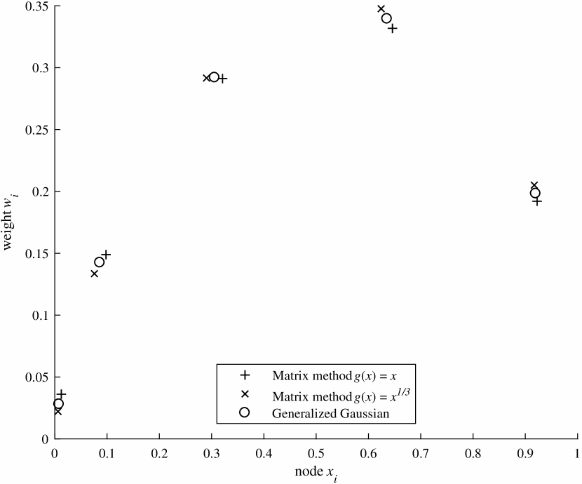
Figure 1: 5-point quadrature rule nodes and weights.

We see from Figure 1 that the three methods give nodes and weights that are close to each other and that the generalized Gaussian quadrature nodes and weights are located between the nodes and weights of the proposed matrix methods.

We compare the accuracy of the methods with a test function $f(x)=x^{y}$ where $y\in[0,6.5]$. Figure 3 shows the relative difference of the exact solution to the quadrature approximation with the three different 5-point rules.

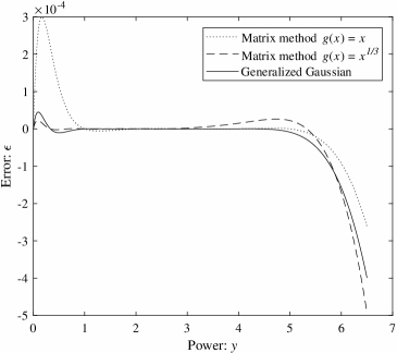
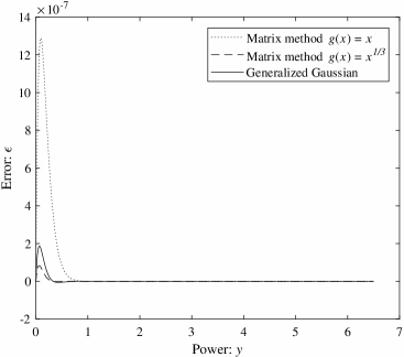
Figure 2: Relative error $\epsilon=\frac{\sum\limits_{k=0}^{4}w_{k}\,x_{k}^{y}}{\int_{0}^{1}x^{y}\,dx}-1$ for the 5-point quadrature rules with $y\in[0,6.5]$.

Figure 3: Relative error $\epsilon=\frac{\sum\limits_{k=0}^{19}w_{k}\,x_{k}^{y}}{\int_{0}^{1}x^{y}\,dx}-1$ for the 20-point quadrature rules with $y\in[0,6.5]$.

We see that the largest errors occur for the small powers and large powers and, on those areas, the generalized Gaussian quadrature is between the matrix method for $g(x)=x$ and $g(x)=\sqrt[3]{x}$. For small powers, $g(x)=\sqrt[3]{x}$ gives the smallest error while for large powers it gives the largest error.

In Figure 3 we see the same comparison for the order 19 matrix method and the generalized Gaussian quadrature where the error is much smaller. Although not shown in Figure 3, the error of the three different methods behaves similarily for large enough values of exponent $y$ as in Figure 3.

The second integral example demonstrates the multiplicative nature of the multiplication operator. The integral is an integral of two variables

$$\int_{0}^{1}\int_{0}^{1}e^{x\,y}\,\log(1+x+y)\,\,dx\,dy.$$

We select the linearly independent basis functions as $\phi_{0}=1,\phi_{1}=x+y,\phi_{2}=x\,y,\phi_{3}=(x+y)^{2},\phi_{4}=(x\,y)^{2},\ldots,\phi_{n-1}=(x+y)^{k},\phi_{n}=(x\,y)^{k}$ and the inner functions for the multiplication operators as $g_{1}=x\,y,g_{2}=x+y$. Then we can approximate the integral as

$$\int_{0}^{1}\int_{0}^{1}e^{x\,y}\,\log(1+x+y)\,\,dx\,dy\approx\left[e^{\boldsymbol{M}_{n}[g_{1}]}\,\log(\boldsymbol{I}+\boldsymbol{M}_{n}[g_{2}])\right]_{0,0}.$$ (17)

This approximation breaks the integral into two different numerical approximations: one given by matrix $\boldsymbol{M}_{n}[g_{1}]$ and the other by $\boldsymbol{M}_{n}[g_{2}]$. These two matrix approximations are used for computing approximations of multiplication operators for two different functions: $e^{g_{1}}$ and $\log(1+g_{2})$ respectively. The final integral approximation uses also other matrix elements of the two multiplication operator approximations besides the $(0,0)$ element as

$$\left[e^{\boldsymbol{M}_{n}[g_{1}]}\,\log(\boldsymbol{I}+\boldsymbol{M}_{n}[g_{2}])\right]_{0,0}=\sum_{k=0}^{n}\left[e^{\boldsymbol{M}_{n}[g_{1}]}\right]_{0,k}\,\left[\log(\boldsymbol{I}+\boldsymbol{M}_{n}[g_{2}])\right]_{k,0}.$$

Again, the matrix approximation of the multiplication operator in terms of orthonormalized functions is computed symbolically. Then we compute the approximation of the integral as a product of the Matlab matrix functions in the 64 bit IEEE 754 floating point. The results of the approximations are shown in Table 1 along with an error estimate. The error estimate is based on a numerical approximation of the integral with Matlab function quad2d. The error bound of the quad2d approximation is $9.7553\cdot 10^{-12}$.

Table 1: Numerical value of approximation (17) for $n+1$ linearly independent functions $\phi_{0},\phi_{1},\ldots,\phi_{n}$.

$n$	$\phi_{n}$	approximation	error
0	$1$	8.900185973444169E-01	5.259050963568923E-02
1	$x+y$	9.382241645325552E-01	4.384942447550944E-03
2	$x\,y$	9.424586790473777E-01	1.504279327284586E-04
3	$(x+y)^{2}$	9.424599771307293E-01	1.491298493768722E-04
4	$x^{2}\,y^{2}$	9.426178212955950E-01	-8.714315488878022E-06
5	$(x+y)^{3}$	9.426129095676246E-01	-3.802587518419998E-06
6	$x^{3}\,y^{3}$	9.426094920018954E-01	-3.850217892287233E-07
7	$(x+y)^{4}$	9.426091679299925E-01	-6.094988636018428E-08
8	$x^{4}\,y^{4}$	9.426091298353442E-01	-2.285523803546852E-08
9	$(x+y)^{5}$	9.426091128176409E-01	-5.837534788888377E-09
10	$x^{5}\,y^{5}$	9.426091104398910E-01	-3.459784903014906E-09
11	$(x+y)^{6}$	9.426091075431513E-01	-5.630451660465496E-10
12	$x^{6}\,y^{6}$	9.426091077121457E-01	-7.320395400967072E-10
13	$(x+y)^{7}$	9.426091069749081E-01	5.198064201294983E-12
14	$x^{7}\,y^{7}$	9.426091070047423E-01	-2.463618198333961E-11
15	$(x+y)^{8}$	9.426091069592208E-01	2.088529349464352E-11
16	$x^{8}\,y^{8}$	9.426091069628073E-01	1.729882903589441E-11
17	$(x+y)^{9}$	9.426091069786899E-01	1.416200490211850E-12
18	$x^{9}\,y^{9}$	9.426091069789710E-01	1.135092020376760E-12

We can see from the table that with about 15 or more basis functions, the numerical integral converges to value of about $0.942609107$ with an absolute error of less than $10^{-10}$.

5 Conclusions

We have introduced a method for numerically approximating integrals as a matrix function of a matrix approximation of a multiplication operator. We have also shown that the new method is a generalization of Gaussian quadrature and that the new quadrature method has similar properties as Gaussian quadrature. Additionally, the convergence was proved for bounded functions. The new method was numerically demonstrated in two examples.

References

- [1] M. Stone, Linear Transformations in Hilbert Space and Their Applications to Analysis, American Mathematical Society, 1932.
- [2] N. Akhiezer, The Classical Moment Problem and Some Related Questions in Analysis, University mathematical monographs, Oliver & Boyd, 1965.
- [3] W. Gautschi, Orthogonal polynomials: applications and computation, Acta Numerica (1996) 45–119.
- [4] W. Gautschi, The interplay between classical analysis and (numerical) linear algebra – a tribute to Gene H. Golub, Electronic Transactions on Numerical Analysis 13 (2002) 119–147.
- [5] W. Gautschi, Orthogonal Polynomials: Computation and Approximation, Numerical mathematics and scientific computation, Oxford University Press, 2004.
- [6] G. Golub, G. Meurant, Matrices, Moments and Quadrature with Applications, Princeton Series in Applied Mathematics, Princeton University Press, 2009.
- [7] B. Simon, Operator Theory, American Mathematical Society, 2015.
- [8] G. H. Golub, J. H. Welsch, Calculation of Gauss quadrature rules, Mathematics of Computation 23 (106) (1969) 221–230.
- [9] D. P. Laurie, Computation of Gauss-type quadrature formulas, J. Comput. Appl. Math. 127 (1-2) (2001) 201–217.
- [10] L. Velázquez, Spectral methods for orthogonal rational functions, Journal of Functional Analysis 254 (4) (2008) 954 – 986.
- [11] M. J. Cantero, R. Cruz-Barroso, P. Gonzáález-Vera, A matrix approach to the computation of quadrature formulas on the unit circle, Applied Numerical Mathematics 58 (3) (2008) 296 – 318.
- [12] R. Cruz-Barroso, S. Delvaux, Orthogonal Laurent polynomials on the unit circle and snake-shaped matrix factorizations, Journal of Approximation Theory 161 (1) (2009) 65 – 87.
- [13] A. Bultheel, M. J. Cantero, A matricial computation of rational quadrature formulas on the unit circle, Numerical Algorithms 52 (1) (2009) 47–68.
- [14] A. Bultheel, P. González-Vera, E. Hendriksen, O. Njåstad, Computation of rational Szegő-Lobatto quadrature formulas, Applied Numerical Mathematics 60 (12) (2010) 1251 – 1263, approximation and extrapolation of convergent and divergent sequences and series (CIRM, Luminy - France, 2009).
- [15] A. Bultheel, M. J. Cantero, R. Cruz-Barroso, Matrix methods for quadrature formulas on the unit circle. A survey, Journal of Computational and Applied Mathematics 284 (2015) 78 – 100.
- [16] K. E. Morrison, Spectral approximation of multiplication operators, New York J. Math 1 (1995) 75–96.
- [17] B. Vioreanu, V. Rokhlin, Spectra of multiplication operators as a numerical tool, SIAM Journal on Scientific Computing 36 (1) (2014) A267–A288.
- [18] B. Vioreanu, Spectra of Multiplication Operators as a Numerical Tool, Yale University, 2012.
- [19] P. Davis, P. Rabinowitz, Methods of Numerical Integration, 2nd Edition, Computer Science and Applied Mathematics, Academic Press, 1984.
- [20] J. Ma, V. Rokhlin, S. Wandzura, Generalized Gaussian quadrature rules for systems of arbitrary functions, SIAM Journal on Numerical Analysis 33 (3) (1996) 971–996.
- [21] J. Weidmann, Linear Operators in Hilbert Spaces, Graduate Texts in Mathematics, Springer-Verlag, 1980.
- [22] I. Segal, R. Kunze, Integrals and Operators, 2nd Edition, Grundlehren der mathematischen Wissenschaften, Springer-Verlag, 1978.
- [23] M. Reed, B. Simon, I: Functional Analysis, revised and enlarged Edition, Methods of Modern Mathematical Physics, Academic Press, 1981.
- [24] N. Akhiezer, I. Glazman, Theory of Linear Operators in Hilbert Space, Dover Books on Mathematics, Dover Publications, 1993.
- [25] I. Segal, Algebraic integration theory, Bull. Amer. Math. Soc. 71 (1965) 419–489.
- [26] N. Higham, Functions of Matrices: Theory and Computation, Society for Industrial and Applied Mathematics, 2008.
- [27] G. H. Golub, C. F. van Loan, Matrix Computations, 3rd Edition, The Johns Hopkins University Press, 1996.
- [28] B. Simon, The Christoffel-Darboux kernel, in: D. Mitrea, M. Mitrea (Eds.), Perspectives in Partial Differential Equations, Harmonic Analysis and Applications: A Volume in Honor of Vladimir G. Maz’ya’s 70th Birthday, American Mathematical Society, 2008, pp. 295–335.
- [29] Y. Yanagisawa, T. Ogita, S. Oishi, A modified algorithm for accurate inverse Cholesky factorization, Nonlinear Theory and Its Applications, IEICE 5 (1) (2014) 35–46.
- [30] K. Ozaki, T. Ogita, S. Oishi, S. M. Rump, Error-free transformations of matrix multiplication by using fast routines of matrix multiplication and its applications, Numerical Algorithms 59 (1) (2012) 95–118.
- [31] R. Bhatia, Matrix Analysis, Graduate Texts in Mathematics, Springer New York, 1997.
- [32] W. G. Bade, Weak and strong limits of spectral operators, Pacific J. Math. 4 (3) (1954) 393–413.
- [33] R. Bartle, D. Sherbert, Introduction to Real Analysis, John Wiley & Sons Canada, Limited, 2011.
- [34] E. Kreyszig, Introductory Functional Analysis with Applications, Wiley Classics Library, John Wiley & Sons, Inc., 1989.
- [35] T. Kato, Perturbation Theory for Linear Operators, 2nd Edition, Classics in Mathematics, Springer Berlin Heidelberg, 1995.