Constructive Preference Elicitation over Hybrid Combinatorial Spaces

Abstract

Preference elicitation is the task of suggesting a highly preferred configuration to a decision maker. The preferences are typically learned by querying the user for choice feedback over pairs or sets of objects. In its constructive variant, new objects are synthesized “from scratch” by maximizing an estimate of the user utility over a combinatorial (possibly infinite) space of candidates. In the constructive setting, most existing elicitation techniques fail because they rely on exhaustive enumeration of the candidates. A previous solution explicitly designed for constructive tasks comes with no formal performance guarantees, and can be very expensive in (or unapplicable to) problems with non-Boolean attributes. We propose the Choice Perceptron, a Perceptron-like algorithm for learning user preferences from set-wise choice feedback over constructive domains and hybrid Boolean-numeric feature spaces. We provide a theoretical analysis on the attained regret that holds for a large class of query selection strategies, and devise a heuristic strategy that aims at optimizing the regret in practice. Finally, we demonstrate its effectiveness by empirical evaluation against existing competitors on constructive scenarios of increasing complexity.

Introduction

Constructive preference elicitation is the task of recommending structured objects, i.e. configurations of several components, assembled on the basis of the user preferences (?; ?). In this setting, the space of possible configurations grows exponentially in the number of components. Examples include configurable products, such as personal computers or mobile phone plans, and complex preference-based decision problems, such as customized travel planning or personalized activity scheduling.

The suggested configurations should reflect the preferences of the user, which are unobserved and must be estimated. As in standard preference elicitation (?), preferences can be learned by iteratively suggesting candidate products to the user, and refining an estimate of the preference model from the received feedback. The ultimate goal is to produce good recommendations with minimal user effort. Here we focus on choice queries, an interaction protocol consisting in recommending a set of products; the user is invited to indicate the most preferred item in the set (?; ?). Elicitation techniques based on choice set queries rely on some strategy to select the next query set to show to the user. Successful query selection strategies must balance between the estimated informativeness of the recommendations (so to minimize the number of elicitation rounds) and their quality (to maximize the chance of the user buying the product and to keep her engaged). By generalizing pairwise ranking feedback, choice queries over larger sets of items allow finer control over informativeness, diversity and quality (?; ?).

Most existing preference elicitation methods are not designed for constructive tasks (?; ?). Regret-based methods (?) rely on perfectly rational user responses, while Bayesian approaches do not scale to combinatorial product spaces (?), as discussed in the related work section. A notable exception is the approach of Teso et al. (?), which avoids the enumeration of the product space by encoding it through mixed-integer linear constraints. Alas, it requires configurations to be encoded with binary variables (in one-hot format), which can be very costly from a computational perspective, and comes with no formal performance guarantees.

In this paper we present several contributions. First, we propose an iterative algorithm, dubbed Choice Perceptron, that generalizes the structured Perceptron (?; ?) to interactive preference elicitation from pairwise and set-wise choice feedback. The query selection strategy is implemented as an optimization problem over the combinatorial space of products. In contrast to previous constructive approaches (?), our algorithm handles general linear utilities over arbitrary feature spaces, including combinatorial and numerical attributes and features. Second, we prove that under a very general assumption (implied by many existing user response models), the expected average regret suffered by our algorithm decreases at least as $\mathcal{O}(1/\sqrt{T})$. We show how the constants appearing in the bound depend on intuitive properties of the query selection strategy, and, as a third contribution, we propose a simple strategy to control these quantities. Our empirical analysis showcases the effectiveness of our approach against several state-of-the-art (including constructive) alternatives.

Related work

Preference elicitation (PE) is a widely studied subject in AI (?; ?). Most existing approaches to PE rely on regret theory (?; ?) or Bayesian estimation (?); see (?) for a brief overview. None of them are suitable for constructive settings, for different reasons. Regret-based methods maintain a version space of utility functions consistent with the collected feedback. However, inconsistent user responses, which are common in real-world recommendation, make the version space collapse. Bayesian methods gracefully deal with inconsistent feedback by employing a full distribution over the candidate utility functions. Unfortunately, selection of the query set (based on optimizing its Expected Value of Information or approximations thereof) is computationally expensive, preventing these approaches from scaling to larger combinatorial domains.

The only approach specifically designed for constructive preference elicitation is SetMargin, introduced in (?). SetMargin can be seen as a max-margin approximation of Bayesian methods that maintains only $k$ most promising candidate utility functions (with $k$ small, e.g. $2$ to $4$). Like the Choice Perceptron, it avoids the explicit enumeration of the product catalogue by compactly defining the latter in terms of MILP constraints, for significant runtime benefits. Alas, it only handles configurations encoded in one-hot form, which can become inefficient for very complex problems involving many categorical variables, relies on a rather involved optimization problem, and it has not be analyzed from a theoretical standpoint. Our query strategy is much simpler, and aims specifically at optimizing an upper bound on the regret.

Our method is related to Coactive Learning (?), which has already found application in constructive tasks (?; ?); some concepts and arguments used in our theoretical analysis are adapted from the Coactive Learning literature (?; ?). However, in our framework the user is asked to choose an option from a set of alternatives, rather than to construct an improved configuration. The two approaches are complementary in the sense that when manipulative feedback is easy to obtain Coactive Learning may be better suited; however when the space of products is highly constrained, producing feasible improvements may be difficult for the user, and our approach is preferable.

Algorithm 1 The Choice Perceptron (cp) algorithm.

1:procedure cp ($T,\eta$)

2:     $\boldsymbol{w}^{1}\leftarrow 0$

3:     for $t=1,\ldots,T$ do

4:         Receive context $x^{t}$ from the user

5:         $\mathcal{Q}^{t}\leftarrow\textsc{SelectQuery}(x^{t},\boldsymbol{w}^{t})$

6:         User chooses $\bar{y}^{t}$ from $\mathcal{Q}^{t}$

7:         $\boldsymbol{w}^{t+1}\leftarrow\boldsymbol{w}^{t}+\eta\Delta^{t}$      

The Choice Perceptron algorithm

We consider a combinatorial space $\mathcal{Y}$ of structured products defined by hard feasibility constraints. As customary in preference elicitation, we focus on the problem of learning a utility function that ranks candidate objects according to the user preferences. The utility of a product $y\!\in\!\mathcal{Y}$ may optionally depend on some externally provided context $x\!\in\!\mathcal{X}$. In the rest of the paper, we assume that the user’s true utility function is fixed and never observed by the algorithm, and that it is linear, i.e. of the form $u^{*}(x,y)=\langle\boldsymbol{w}^{*},\boldsymbol{\phi}(x,y)\rangle$; here $\boldsymbol{w}^{*}\!\in\!\mathbb{R}^{d}$ are the true preference weights of the user and $\boldsymbol{\phi}:\mathcal{X}\!\times\!\mathcal{Y}\rightarrow\mathbb{R}^{d}$ maps context-configuration pairs to a $d$-dimensional feature space. The feature vectors $\boldsymbol{\phi}(x,y)$ are assumed to be enclosed in a ball of radius $R$.

We propose the Choice Perceptron (cp) algorithm; the pseudocode is listed in Algorithm 1. The cp algorithm keeps an estimate $u^{t}(x,y)=\langle\boldsymbol{w}^{t},\boldsymbol{\phi}(x,y)\rangle$ of the true user utility, and iteratively refines it by interacting with the user. At each iteration $t$, the algorithm receives a context $x^{t}$ and recommends a set of $k$ configurations $\mathcal{Q}^{t}\!\subseteq\!\mathcal{Y}$, by selecting them according to some query strategy based on $\boldsymbol{w}^{t}$. After receiving the query set, the user chooses the “best” object $\bar{y}^{t}\!\in\!\mathcal{Q}^{t}$ according to her preferences. This kind of set-wise interaction protocol generalizes pairwise ranking feedback, and is well studied in decision theory, psychology, and econometrics (?; ?; ?). We allow the choice to be noisy, i.e. the user may choose $\bar{y}^{t}$ according to a distribution $P_{x^{t}}(\bar{y}^{t}\!=\!y|y\in\mathcal{Q}^{t})$.

After observing the user’s pick, the algorithm updates the current estimate $\boldsymbol{w}^{t}$. Here we focus on the following Perceptron update:

$$\boldsymbol{w}^{t+1}\leftarrow\boldsymbol{w}^{t}+\eta\Delta^{t}$$

$$\Delta^{t}:=\boldsymbol{\phi}(x^{t},\bar{y}^{t})-\frac{1}{k-1}\sum_{y\in\mathcal{Q}^{t}:y\neq\bar{y}^{t}}\boldsymbol{\phi}(x^{t},y)$$ (1)

where $\eta$ is a constant step-size. Despite its simplicity, this update comes with sound theoretical guarantees, as shown in the next section.

We measure the quality of a recommendation set $\mathcal{Q}^{t}$ in context $x^{t}$ by the instantaneous regret, that is the difference in true utility between a truly optimal object $y^{*}_{x^{t}}\!=\!\operatorname*{argmax}_{y\in\mathcal{Y}}u^{*}(x^{t},y)$ and the best option in the set:

$$\text{REG}(x^{t},\mathcal{Q}^{t})=\min_{y\in\mathcal{Q}^{t}}\left(u^{*}(x^{t},y^{*}_{x^{t}})-u^{*}(x^{t},y)\right)$$

This definition is in line with previous works on preference elicitation with set-wise choice feedback (?). After $T$ iterations, the average regret is $\text{REG}^{T}\!=\!\frac{1}{T}\sum_{t=1}^{T}\text{REG}(x^{t},\mathcal{Q}^{t})$. A low average regret implies low instantaneous regret throughout the elicitation process, as is necessary for keeping the user engaged. In the next section we prove a theoretical upper bound on the expected average regret suffered by cp under a very general assumption on the user feedback.

Theoretical Analysis

In this section we analyze the theoretical properties of the cp algorithm, proving an $\mathcal{O}(1/\sqrt{T})$ upper bound on its expected average regret. In the following $\mathbb{E}_{\bar{y}^{t}}[f(x^{t},y)|\mathcal{Q}^{t}]$ indicates the conditional expectation of $f(x^{t},y)$ with respect to $P_{x^{t}}(\bar{y}^{t}\!=\!y|\mathcal{Q}^{t})$, where $t$ is the iteration index; $\mathbb{E}[f(x^{t},y)]$ is the expectation of $f(x^{t},y)$ over the distribution of all user choices $\bar{y}^{1},\ldots,\bar{y}^{t}$. We will also use the shorthands $P_{t}(y):=P_{x^{t}}(\bar{y}^{t}\!=\!y|y\in\mathcal{Q}^{t})$, $u^{*}(\Delta^{t}):=\langle\boldsymbol{w}^{*},\Delta^{t}\rangle$ and $[k]:=\{1,\dots,k\}$.

In order to derive the regret bound, we need to quantify the “quality” of the sets provided by the query strategy. To this end, we adapt the concept of expected $\alpha$-informativeness from the Coactive Learning framework (?):

Definition.

For any query strategy, there exist $\alpha\in(0,1]$ and $\bar{\xi}^{t}\in\mathbb{R}$ such that, for all $t\in[T]$ and for all users:

$$\mathbb{E}_{\bar{y}^{t}}[u^{*}(\Delta^{t})|\mathcal{Q}^{t}]\geq$$

$$\qquad\qquad\alpha\max_{y\in\mathcal{Q}^{t}}\left(u^{*}(x^{t},y^{*}_{x^{t}})-u^{*}(x^{t},y)\right)-\bar{\xi}^{t}$$ (2)

The LHS of Eq. 2 is the expected utility gain of the update rule (Eq. 1): a positive utility gain indicates that $\boldsymbol{w}^{t+1}$ makes a step towards a better approximation of $\boldsymbol{w}^{*}$. The term $\max_{y\in\mathcal{Q}^{t}}\left(u^{*}(x^{t},y^{*}_{x^{t}})-u^{*}(x^{t},y)\right)$ on the RHS is instead the worst-case regret, i.e. the regret with respect to the worst object in the query set. This model simply quantifies the amount of utility gain in terms of a fraction $\alpha$ of the worst-case regret and the slack term $\bar{\xi}^{t}$. Intuitively, $\alpha$ captures the minimum quality of the query sets selected by the query strategy, while the slacks $\bar{\xi}^{t}$ are additional degrees of freedom that depend on the expected user replies.

Notice that the above definition is very general and can describe the behavior of any query selection strategy, provided appropriate values for $\alpha$ and $\bar{\xi}^{t}$. Both occur as constants in our regret bound.

By requiring the user to behave “reasonably”, according to the following definition, we can guarantee the expected utility gain to always be non-negative (Lemma 1). This allows us to make explicit and assign a precise meaning to the value of the constant $\bar{\xi}^{t}$.

Definition.

A user is reasonable if, for any context $x^{t}$ and query set $\mathcal{Q}^{t}$, the probability $P_{x^{t}}(\bar{y}^{t}\!=\!y|\mathcal{Q}^{t})$ is a non-decreasing monotonic transformation of the true utility $u^{*}$:

$$\forall y,y^{\prime}\!\in\!\mathcal{Q}^{t}\quad P_{t}(y)\geq P_{t}(y^{\prime})\iff u^{*}(x^{t},y)\geq u^{*}(x^{t},y^{\prime})$$

This property is implied by many widespread user response models, including the Bradley-Terry (?) and Thurstone-Mosteller (?) models of pairwise choice feedback, and the Plackett-Luce (?; ?) model of set-wise choice feedback. It is also strictly less restrictive than applying any of these models.

Notably, when applied to a reasonable user, the update rule (Eq. 1) always yields a non-negative expected utility gain.

Lemma 1.

For a reasonable user with utility $u^{*}$, it holds that $\mathbb{E}_{\bar{y}^{t}}[u^{*}(\Delta^{t})|\mathcal{Q}^{t}]\geq 0$ at all iterations $t$.

Proof.

Given that the user is reasonable, we apply the Chebyshev’s sum inequality to $u^{*}(x^{t},y^{t})$ and $P_{x^{t}}(\bar{y}^{t}\!=\!y^{t}|\mathcal{Q}^{t})$, for $y^{t}\in\mathcal{Q}^{t}$:

$$\textstyle\frac{1}{k}\sum_{y^{t}\in\mathcal{Q}^{t}}u^{*}(x^{t},y^{t})P_{t}(y^{t})\geq$$

$$\textstyle\qquad\left(\frac{1}{k}\sum_{y^{t}\in\mathcal{Q}^{t}}u^{*}(x^{t},y^{t})\right)\cdot\left(\frac{1}{k}\sum_{y^{t}\in\mathcal{Q}^{t}}P_{t}(y^{t})\right)$$

$$\Longleftrightarrow\quad \textstyle\sum_{y^{t}\in\mathcal{Q}^{t}}u^{*}(x^{t},y^{t})P_{t}(y^{t})\geq\frac{1}{k}\sum_{y^{t}\in\mathcal{Q}^{t}}u^{*}(x^{t},y^{t})$$

Rearranging, we obtain:

$$\textstyle\sum_{y^{t}\in\mathcal{Q}^{t}}u^{*}(x^{t},y^{t})P_{t}(y^{t})-\frac{1}{k}\sum_{y^{t}\in\mathcal{Q}^{t}}u^{*}(x^{t},y^{t})\geq 0$$

$$\Longleftrightarrow \textstyle\quad\frac{k}{k-1}\mathbb{E}[u^{*}(x^{t},\bar{y}^{t})|\mathcal{Q}^{t}]-\frac{1}{k-1}\sum_{y^{t}\in\mathcal{Q}^{t}}u^{*}(x^{t},y^{t})\geq 0$$

$$\Longleftrightarrow \textstyle\quad\mathbb{E}[\frac{k}{k-1}u^{*}(x^{t},\bar{y}^{t})-\frac{1}{k-1}\sum_{y^{t}\in\mathcal{Q}^{t}}u^{*}(x^{t},y^{t})|\mathcal{Q}^{t}]\geq 0$$

$$\Longleftrightarrow \textstyle\quad\mathbb{E}[\frac{k-1}{k-1}u^{*}(x^{t},\bar{y}^{t})-\frac{1}{k-1}\sum_{y^{t}\neq\bar{y}^{t}}u^{*}(x^{t},y^{t})|\mathcal{Q}^{t}]\geq 0$$

$$\Longleftrightarrow \textstyle\quad\mathbb{E}[u^{*}(x^{t},\bar{y}^{t})-\frac{1}{k-1}\sum_{y^{t}\neq\bar{y}^{t}}u^{*}(x^{t},y^{t})|\mathcal{Q}^{t}]\geq 0$$

∎

The lemma allows us to distinguish between informative and uninformative query sets, depending on whether the expected utility gain is strictly positive or null, respectively. We can use these definitions to derive an equivalent formulation of the $\alpha$-informativeness making the constants $\bar{\xi}^{t}$ explicit.

Let $\alpha>0$ be the smallest constant such that $\mathbb{E}_{\bar{y}^{t}}[u^{*}(\Delta^{t})|\mathcal{Q}^{t}]\!\geq\!\alpha\max_{y\in\mathcal{Q}^{t}}\left(u^{*}(x^{t},y^{*}_{x^{t}})-u^{*}(x^{t},y)\right)$ for all iterations $t$ in which the query set $\mathcal{Q}^{t}$ is informative. For these iterations setting $\bar{\xi}^{t}=0$ still satisfies the inequality in Eq. 2. On the other hand, when the query set is uninformative, $\bar{\xi}^{t}$ must satisfy $\bar{\xi}^{t}\!\geq\!\alpha\max_{y\in\mathcal{Q}^{t}}\left(u^{*}(x^{t},y^{*}_{x^{t}})-u^{*}(x^{t},y)\right)$. Given that $\lVert\boldsymbol{\phi}(x,y)\rVert\leq R$, the worst-case regret is upper-bounded by $2R\lVert\boldsymbol{w}^{*}\rVert$, therefore it suffice to set $\bar{\xi}^{t}\!=\!2\alpha R\lVert\boldsymbol{w}^{*}\rVert$. We can rewrite the expected $\alpha$-informativeness as:

$$\mathbb{E}_{\bar{y}^{t}}[u^{*}(\Delta^{t})|\mathcal{Q}^{t}]\geq$$

$$\quad\alpha\max_{y\in\mathcal{Q}^{t}}\left(u^{*}(x^{t},y^{*}_{x^{t}})-u^{*}(x^{t},y)\right)-2\alpha R\lVert\boldsymbol{w}^{*}\rVert m^{t}$$ (3)

Here $m^{t}\!=\!\mathds{1}[\mathbb{E}[u^{*}(\Delta^{t})]\!=\!0]$ is a constant that is equal to $1$ if any query set $\mathcal{Q}^{t}$ that may be chosen at iteration $t$ is expected to be uninformative and $0$ otherwise. Note that $\mathbb{E}[u^{*}(\Delta^{t})]=\mathbb{E}[\mathbb{E}_{\bar{y}^{t}}[u^{*}(\Delta^{t})|\mathcal{Q}^{t}]]$, therefore if $\mathcal{Q}^{t}$ is informative then $\mathbb{E}[u^{*}(\Delta^{t})]>0$ (i.e. $m^{t}\!=\!0$), while if $\mathcal{Q}^{t}$ is uninformative then $\mathbb{E}[u^{*}(\Delta^{t})]=0$ (i.e. $m^{t}\!=\!1$). We say that an iteration $t$ is expected uninformative if $m^{t}\!=\!1$, and let $M\!:=\!\sum_{t=1}^{T}m^{t}$ be the total number of expected uninformative iterations.

The last property of the query selection strategy we define in order to state the bound is the $\beta$-affirmativeness, which we adapt from (?) as follows:

Definition.

For any query selection strategy and for a fixed time horizon $T$, there exists a constant $\beta\in\mathbb{R}$ such that $\frac{1}{T}\sum_{t=1}^{T}\mathbb{E}[u^{t}(\Delta^{t})]\leq\beta$.

This definition states that $\beta$ is an upper bound on the average expected change in $u^{t}$, for $t\in[T]$. Notice that $\mathbb{E}[u^{t}(\Delta^{t})]$ may be positive, null or negative. Intuitively, a negative $\mathbb{E}[u^{t}(\Delta^{t})]$ indicates that the query set is expected to produce a user choice that disagrees with the current estimate of $\boldsymbol{w}^{t}$. This is the case in which the algorithm receives the most information. In general, the smaller $\beta$ is, the quicker cp learns from the user feedback.

The previous assumptions on the user and definitions for the query strategy allow us to derive the following regret bound for cp along the same lines of what done in Coactive Learning (?; ?).

Theorem 2.

For a reasonable user with true preference weights $\boldsymbol{w}^{*}$ and an $\alpha$-informative and $\beta$-affirmative query strategy, the expected average regret of the cp algorithm is upper bounded by:

$$\mathbb{E}[\text{REG}^{T}]\leq\frac{\sqrt{2\frac{\beta}{\eta}+4R^{2}}\|\boldsymbol{w}^{*}\|}{\alpha\sqrt{T}}+\frac{2R\lVert\boldsymbol{w}^{*}\rVert M}{T}$$

Proof.

Using Cauchy-Schwarz and Jensen’s inequalities:

$$\mathbb{E}[\langle\boldsymbol{w}^{*},\boldsymbol{w}^{T+1}\rangle] \leq\|\boldsymbol{w}^{*}\|\;\mathbb{E}[\|\boldsymbol{w}^{T+1}\|]$$

$$\leq\|\boldsymbol{w}^{*}\|\;\sqrt{\mathbb{E}[\langle\boldsymbol{w}^{T+1},\boldsymbol{w}^{T+1}\rangle]}$$ (4)

From the expected $\beta$-affirmativeness and $\lVert\boldsymbol{\phi}(x,y)\rVert\leq R$:

$$\mathbb{E}[\langle\boldsymbol{w}^{T+1},\boldsymbol{w}^{T+1}\rangle]=$$

$$\quad=\mathbb{E}[\langle\boldsymbol{w}^{T},\boldsymbol{w}^{T}\rangle]+2\eta\mathbb{E}[\langle\boldsymbol{w}^{T},\Delta^{T}\rangle]+\eta^{2}\mathbb{E}[\langle\Delta^{T},\Delta^{T}\rangle]$$

$$\quad\leq 2\eta\sum_{t=1}^{T}\mathbb{E}[\langle\boldsymbol{w}^{t},\Delta^{t}\rangle]+4\eta^{2}R^{2}T\leq 2\eta\beta T+4\eta^{2}R^{2}T$$

Plugging this result into inequality (4) we have:

$$\mathbb{E}[\langle\boldsymbol{w}^{*},\boldsymbol{w}^{T+1}\rangle]\leq\sqrt{2\eta\beta T+4\eta^{2}R^{2}T}\|\boldsymbol{w}^{*}\|$$

For a reasonable user, the $\alpha$-informativeness in Eq. 3 holds for any query strategy. Applying it to the LHS of the above inequality, along with the law of total expectation, we get:

$$\textstyle\mathbb{E}[\langle\boldsymbol{w}^{*},\boldsymbol{w}^{T+1}\rangle]$$

$$=\ \textstyle\mathbb{E}[\langle\boldsymbol{w}^{*},\boldsymbol{w}^{T}\rangle]+\eta\mathbb{E}[\mathbb{E}_{\bar{y}^{T}}[\langle\boldsymbol{w}^{*},\Delta^{T}\rangle|\mathcal{Q}^{t}]]$$

$$=\ \textstyle\mathbb{E}[\sum_{t=1}^{T}\eta\mathbb{E}_{\bar{y}^{t}}[u^{*}(\Delta^{t})|\mathcal{Q}^{t}]]$$

Applying the $\alpha$-informativeness (Eq. 3):

$$\geq\ \textstyle\alpha\eta\mathbb{E}[\sum_{t=1}^{T}\max_{y\in\mathcal{Q}^{t}}\left(u^{*}(x^{t},y^{*}_{x^{t}})-u^{*}(x^{t},y)\right)]$$

$$\textstyle\qquad-2R\alpha\eta\lVert\boldsymbol{w}^{*}\rVert\sum_{t=1}^{T}m^{t}$$

$$\geq\ \textstyle\alpha\eta\mathbb{E}[\sum_{t=1}^{T}\min_{y\in\mathcal{Q}^{t}}\left(u^{*}(x^{t},y^{*}_{x^{t}})-u^{*}(x^{t},y)\right)]$$

$$\textstyle\qquad-2R\alpha\eta\lVert\boldsymbol{w}^{*}\rVert\sum_{t=1}^{T}m^{t}$$

$$=\ \textstyle\alpha\eta T\mathbb{E}[\text{REG}^{T}]-2R\alpha\eta\lVert\boldsymbol{w}^{*}\rVert M$$

Finally:

$$\alpha\eta T\mathbb{E}[\text{REG}^{T}]$$

$$\leq\ \sqrt{2\eta\beta+4\eta^{2}R^{2}}\|\boldsymbol{w}^{*}\|\sqrt{T}+2R\alpha\eta\lVert\boldsymbol{w}^{*}\rVert M$$

from which the claim follows. ∎

Query selection strategy

In the previous section we proved an upper bound on the expected average regret of cp for any query selection strategy, provided that the user is reasonable. Crucially, however, the bound depends on the actual value of $\alpha$, $\beta$ and $M$. These constants depend both on the user and the query selection strategy. While the algorithm has no control on the user, an appropriate design of the query selection strategy can positively affect the impact of the constants on the bound. In the following we present a query selection strategy that aims at reducing the bound by finding a trade-off between $\alpha$ and $\beta$.

Recall that we want $\alpha\in(0,1]$ to be large and $\beta\in\mathbb{R}$ and $M\in[T]$ small. While have no direct control over $\alpha$ and $\beta$, which depend on all iterations, we can control their step-wise surrogates:

$$\textstyle u^{*}(\Delta^{t}) =\textstyle\langle\boldsymbol{w}^{*},\Delta^{t}\rangle\propto\|\boldsymbol{w}^{*}\|\|\Delta^{t}\|\;\;\text{for $\alpha$}$$

$$\textstyle u^{t}(\Delta^{t}) =\textstyle\langle\boldsymbol{w}^{t},\Delta^{t}\rangle\propto\|\boldsymbol{w}^{t}\|\|\Delta^{t}\|\;\;\text{for $\beta$}$$

There is a trade-off between the two, as they both depend on $\|\Delta^{t}\|$. Further, while $\boldsymbol{w}^{t}$ is observed, $\boldsymbol{w}^{*}$ is not. We proceed as follows. Since $\boldsymbol{w}^{*}$ is not observed, we indirectly maximize $u^{*}(\Delta^{t})$ by maximizing $\|\Delta^{t}\|$, i.e. by picking $k$ query configurations that are distant in feature space. For reasonable users, maximizing the distance between objects also tends to maximize the probability $P_{t}(y)$ of picking a high utility object: the larger the distance, the higher the probability of picking objects with large difference in $u^{*}(\cdot)$. On the other hand $\boldsymbol{w}^{t}$ is observed, so we can choose $k$ query configurations with small difference in estimated utility $u^{t}(\cdot)$ by taking them from a plane orthogonal (or almost orthogonal) to $\boldsymbol{w}^{t}$. This way, $u^{t}(\Delta^{t})$ is close to $0$ regardless of the choice of the user, implying $\beta\approx 0$. This reasoning leads to the following optimization problem:

$$\mathcal{Q}^{t}=\operatorname*{argmax}_{\{y_{1},\dots,y_{k}\}} \quad\gamma\delta+(1-\gamma)\mu$$

s.t. $$\textstyle u^{t}(x^{t},y_{1})\!=\!\max_{y}u^{t}(x^{t},y)$$

$$\textstyle\boldsymbol{\phi}(x^{t},y_{1})\neq\dots\neq\boldsymbol{\phi}(x^{t},y_{k})$$

where: $$\textstyle\delta:=\sum_{i=2}^{k}\lVert\boldsymbol{\phi}(x^{t},y_{1})-\boldsymbol{\phi}(x^{t},y_{i})\rVert_{1}$$

$$\textstyle\mu:=\sum_{i=2}^{k}u^{t}(x^{t},y_{j})$$

The objective aims at optimizing a convex combination of the $L_{1}$ distances of the options in $\mathcal{Q}$ ($\delta$) and their distance from optimality ($\mu$). The two terms are modulated by the $\gamma\in[0,1]$ hyperparameter. The third constraint forces the first configuration $y_{1}$ to be optimal, irrespective of the choice of $\gamma$, ensuring that when $\boldsymbol{w}^{t}\approx\boldsymbol{w}^{*}$, $\mathcal{Q}^{t}$ contains at least one true optimal configuration. Finally, all options are required to be different in feature space. By maximizing the utility of the objects, we are also pushing $\mathbb{E}[\langle\boldsymbol{w}^{t},\Delta^{t}\rangle]$ towards zero, implying that iteration $t$ can only be expected uninformative when $\boldsymbol{w}^{t}$ is (approximately) anti-parallel to $\boldsymbol{w}^{*}$:

$$\mathbb{E}[u^{*}(\Delta^{t})]=0\iff\mathbb{E}[\langle\boldsymbol{w}^{*},\boldsymbol{w}^{t}\rangle]\approx-\mathbb{E}[\lVert\boldsymbol{w}^{*}\rVert\lVert\boldsymbol{w}^{t}\rVert]$$

For reasonable users $\mathbb{E}[\langle\boldsymbol{w}^{*},\boldsymbol{w}^{t}\rangle]=\mathbb{E}[\sum_{t=1}^{T}u^{*}(\Delta^{t})]\geq 0$ (by Lemma 1), implying that the above case is extremely rare, and therefore $M\approx 0$.

This query strategy essentially attempts to find a good trade-off between exploration ($\gamma\approx 1$) and exploitation ($\gamma\approx 0$). In most cases a good strategy is to allow more exploration in the beginning of the elicitation and then exploit more when the algorithm has learned a good approximation of $\boldsymbol{w}^{*}$. We therefore set $\gamma$ to $\frac{1}{t}$ in our experiments. This also ensures that $u^{t}(\Delta^{t})$ decreases over time regardless of the user choice, thereby keeping $\beta$ constant.

In the following, we will stick to features $\boldsymbol{\phi}$ expressible as linear functions of Boolean, categorical and continuous attributes. This choice is very general, and allows to encode arithmetical, combinatorial and logical constraints, as shown by our empirical evaluation. So long as the feasible set $\mathcal{Y}$ is also defined in terms of mixed linear constraint, query selection can be cast as a mixed-integer linear problem (MILP) and solved with any efficient off-the-shelf solver.

We remark that the previous arguments apply to all choices of $k\geq 2$, i.e. to both pairwise and set-wise choice feedback. Intuitively, larger set sizes imply more diverse and potentially more informative query sets, because they reduce the chance for a reasonable user to pick a low utility option. They also imply more conservative updates, mitigating the deleterious effect of uninformative choices. These effects are studied experimentally.

Empirical Evaluation

We compare cp against three state-of-the-art preference elicitation approaches on three constructive preference elicitation tasks taken from the literature. The query selection problem is solved with Gecode via its MiniZinc interface (?).

The three competitors are: [i] the Bayesian approach of (?) using Monte Carlo methods (the number of particles was set to 50,000, as in (?)) with greedy query selection based on the Expected Utility of a Selection (a tight approximation of the Expected Value of Information criterion); [ii] Query Iteration, also from (?), a sampling-based query selection method that trades off query informativeness for computational efficiency; [iii] the set-wise maximum margin method of (?), modified to accept set-wise choice feedback; support for user indifference was also disabled. We indicate the competitors as vb-eus, vb-qi and SetMargin, respectively. As argued in the previous section, for cp we set $\gamma$ to $\frac{1}{t}$ in all experiments, in order to allow more exploration earlier on during the search. In practice we also employ an adaptive Perceptron step size, which is adapted at each iteration $t\geq 3$ from the set $\{0.1,0.2,0.5,1,2,5,10\}$ via cross-validation on the collected feedback; it was found to work well empirically. SetMargin includes a similar tuning procedure.

Our experimental setup is modelled after (?). We consider two different kinds of users: “uniform” and “normal” users, whose true preference vectors $\boldsymbol{w}^{*}$ are drawn, respectively, from a uniform and a normal distribution. Twenty users are sampled at random and kept fixed for each experiment. User responses are simulated with a Plackett-Luce model (?; ?):

$$P_{x}(\bar{y}=y_{i}|\mathcal{Q})=\frac{\exp(\lambda u^{*}(x,y_{i}))}{\sum_{j=1}^{k}\exp(\lambda u^{*}(x,y_{j}))}$$

We set $\lambda=1$ as in (?). In the first two experiments (which are context-less) we report the median over users of the instantaneous regret, as in (?) and (?); whereas, in the third experiment (with context) we report the median average regret. In all experiments we also report cumulative runtime and standard deviations.

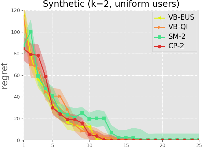
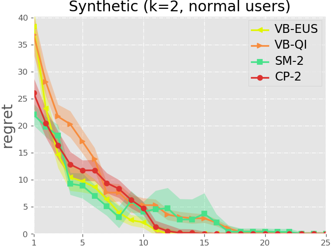
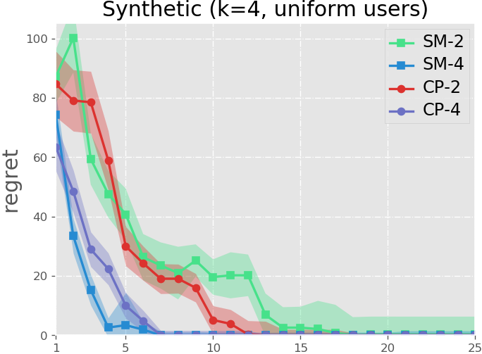
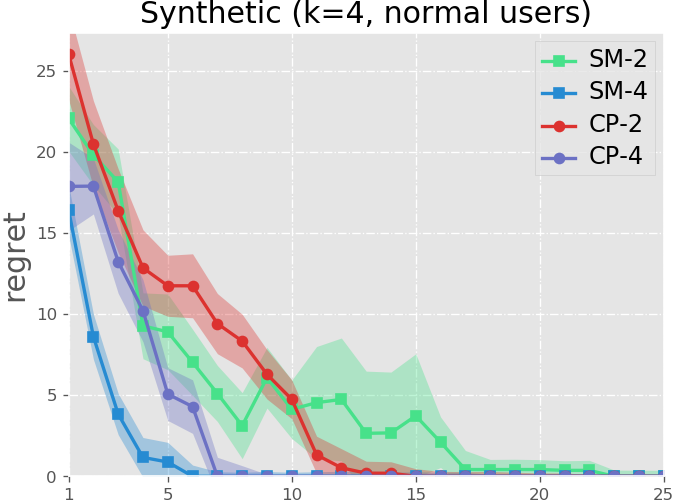
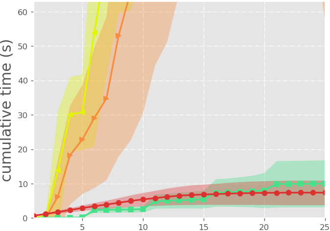
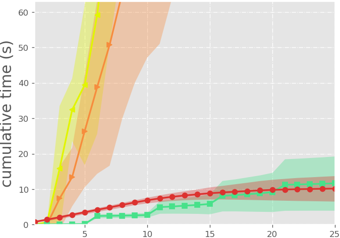
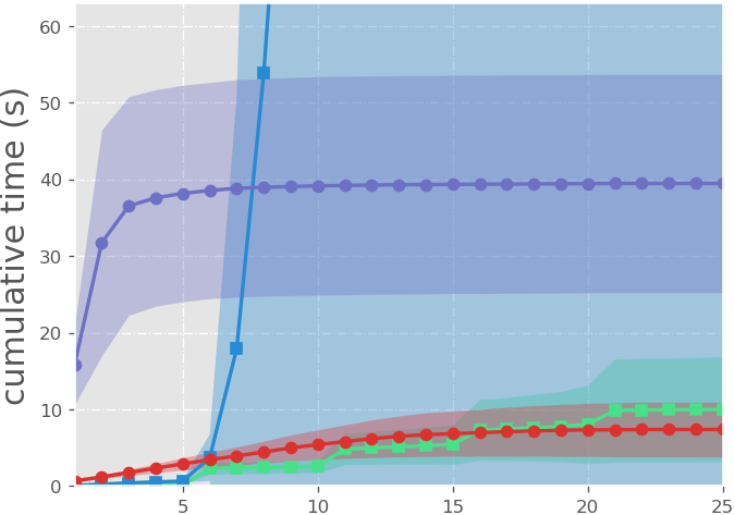
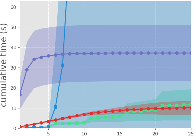
Figure 1: Comparison of various algorithms in the synthetic experiment. The plots on the top row show the regret of the various algorithm for increasing iterations, whereas the plots on the bottom row show the cumulative running time (inference + learning). On the left, cp is compared to SetMargin, vb-eusand vb-qiusing query sets with dimension $k=2$. On the right, instead, cp is compared only with SetMargin using $k=4$. In both cases, experiments using uniformly distributed and normally distributed users are shown on the left plots and on the right plots respectively. Best viewed in color.

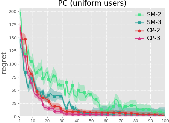
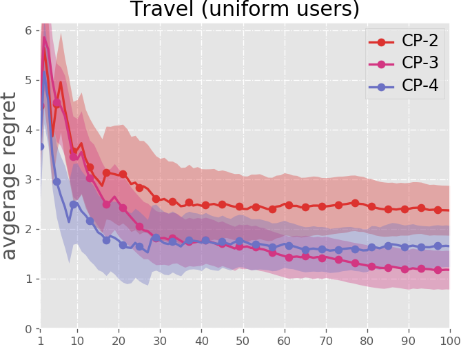
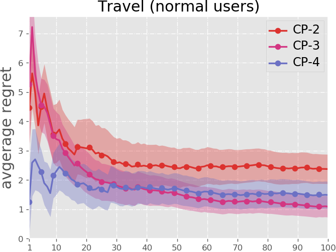
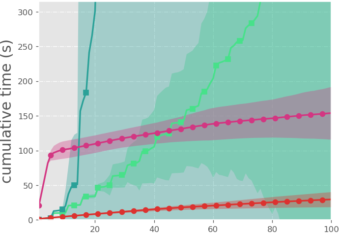
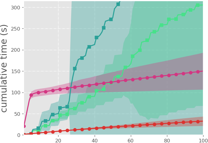
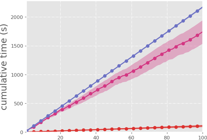
Figure 2: Comparison of various algorithms in the PC configuration and travel planning experiments. The plots on the top row show the regret of the various algorithm for increasing iterations, whereas the plots on the bottom row show the cumulative running time (inference + learning). On the left, cp is compared to SetMargin on the PC configuration task using query sets with dimension $k=2$ and $k=3$. The plots on the right, instead, show only the performance of cp on the travel planning task using $k=\{2,3,4\}$. In both cases, experiments using uniformly distributed and normally distributed users are shown on the left plots and on the right plots respectively. Best viewed in color.

Synthetic experiment.

We evaluated all methods on the synthetic constructive benchmark introduced in (?). The space of feasible configurations is the Cartesian product of $r$ attributes, each taking values in $[r]$, i.e. $\mathcal{Y}=\times_{i=1}^{r}[r]$. The features are the one-hot encoding of the attributes, for a total of $r^{2}$ features. Here we focus on the $r=4$ case ($16$ features, $256$ products) which is large enough to be non-trivial, and sufficiently small to be solvable by the two Bayesian competitors. For cp and SetMargin  $\mathcal{Y}$ is encoded natively via MILP constraints; the Bayesian methods required $\mathcal{Y}$ to be enumerated. The users were sampled as in (?), i.e. from a uniform distribution in the range $[1,100]$ and a normal distribution with mean $25$ and standard deviation $\frac{25}{3}$. All methods were run until either the user was satisfied (i.e. the regret reported by the method reached zero) or 25 iterations elapsed. We evaluated the importance of the query set size by running cp and SetMargin with $k=2,3,4$. vb-eus and vb-qi were only run with $k=2$, due to scalability issues. In the $k=2$ case (Figure 1, left), cp performs better than both vb-qi and SetMargin, and worse than vb-qi. The runtimes, however, vary wildly. The Bayesian competitors are much more computationally expensive than cp and SetMargin, confirming the results of (?); the two MILP methods instead avoid the explicit enumeration of the candidate configurations, with noticeable computational savings. Notably, cp is faster than SetMargin, while performing comparably or better. The gap widens with set size $k=4$ (Figure 1, right; $k=3$ is similar, not shown). Here cp and SetMargin converge after a similar number of iterations, but with very different runtimes. The bottleneck of SetMargin is the hyperparameter tuning procedure; disabling it however severely degrades the performance, so we left it on.

PC configuration.

In the second experiment, we compared cp and SetMargin on a much larger recommendation task, also from (?). The goal is to suggest a fully customized PC configuration to a customer. A computer is defined by seven categorical attributes (manufacturer, CPU model, etc.) and a numerical one (the price, determined by the choice of components). The features include the one-hot encodings of the attributes and the price. The relations between parts (e.g. what CPUs are sold by which manufacturers) are expressed as Horn constraints. The feasible space includes thousands of configurations, ruling the Bayesian competitors out (?). The users were sampled as in the previous experiment. To help keeping running times low, the query selection procedure of cp is executed with a 20 seconds time cutoff. No time cutoff is applied to SetMargin.

The results for $k=2$ and $3$ can be seen in Figure 2 (left). On uniform users, cp consistently outperforms SetMargin for both choices of $k$, despite the timeout. Notably, cp with $k=2$ (less informative queries) works as well as SetMargin with $k=3$ (more informed queries) in this setting. For normal users the situation is similar: with $k=2$, SetMargin catches up with cp after about 80 iterations, but at considerably larger computational cost. Surprisingly, SetMargin behaves worse for $k=3$ than for $k=2$; cp instead improves monotonically, for a modest increase in computational effort. In all cases, the runtimes are very favorable to our method, also thanks to the timeout, which however does not compromise performance.

Trip planning.

Finally, we evaluated cp on a slightly modified version of the touristic trip planning task introduced in (?). Here the recommender must suggest a trip route between 10 cities, each annotated with an offering of 15 activities (resorts, services, etc.). The trip $y$ includes the path itself (which is allowed to contain cycles) and the time spent at each city. Differently from (?), at each iteration the user issues a context $x$ indicating a subset of cities that the trip must visit. The features include the number of days spent at each location, the number of times an activity is available at the visited locations, the cost of the trip, etc., for a total of 127 features; see (?) for the details. Note that this problem can not be encoded in SetMargin, i.e. with Boolean and dependent numerical attributes, without incurring significant encoding overhead: the resulting SetMargin query selection problem would include approximately 300 Boolean variables (an almost 300% blow-up in problem size). According to our tests, problems of this size are not solvable in real-time in practice, compromising the reactiveness of SetMargin.

Differently from the previous two settings, here users were sampled from a standard normal distribution (as in (?)) and from a uniform distribution in the range $[-1,1]$. Not having a one-hot encoded feature vector, negative weights are useful to capture the user dislikes. The contexts are uniformly sampled from the combinations of 2 or 3 cities. As in the previous experiment, we employ a time cutoff of 20 seconds. We run this experiment with $k={2,3,4}$ to show how different set sizes affect the performance of the system. Since this experiment is context-based, we let the algorithm run for exactly 100 iterations. Figure 2 (right) reports the median average regret and the median cumulative running time.

The plots show that in both cases there is a significant decrease in average regret with $k=3$ over $k=2$, in exchange for increased running time; $k=4$ performs better than $k=3$ for about 40 iterations, but then worsens considerably. This is probably due to the timeout, which in this more complicated setting may substantially hinder the MILP solver. Increasing the cutoff to 60 seconds however did not improve the results (data not shown). This indicates that larger values of $k$ may be too costly to compute without further approximations, as is also the case for the other competitors.

Choosing $k$

While our theoretical analysis is agnostic on the number $k$ of objects in a query set, in our empirical analysis we collected some insight on how to choose $k$ on the basis of the difficulty of the underlying optimization problem. While in general a larger $k$ is more informative, it is not always possible to solve the query selection problem to optimality. This may severely hinder the learning capabilities of the algorithm, as in the case of the trip planning setting with $k=4$. On the other hand, for smaller problems a larger $k$ may significantly reduce the number of iterations needed to reach an optimal solution, as for the PC configuration setting. There is, therefore, a trade-off that depends on the computational complexity of the query selection problem of the application at hand. From our experiments, we can infer, as a rule of thumb, that it is usually better to choose larger $k$ ($k=4,5$) when objects are small and the selection problem easier to solve, whereas a smaller $k$ ($k=2,3$) is preferable when the objects are large and difficult to select. Additionally, the larger the objects, the harder it is for the user to choose the best in the set, so a smaller $k$ is also desirable to reduce the cognitive load on the user.

Conclusion

We presented the Choice Perceptron, an algorithm for preference elicitation from noisy choice feedback. Contrary to existing recommenders, cp can solve constructive elicitation problems over arbitrary combinatorial spaces, composed of many Boolean, integer and continuous variables and constraints. Our theoretical analysis shows that, under a very general assumption, the average regret suffered by cp is upper bounded by $\mathcal{O}(1/\sqrt{T})$. The exact constants appearing in the bound depend on intuitive properties of the query selection strategy at hand. We further described a strategy that aims at controlling these constants. We applied cp to constructive preference elicitation tasks for progressively more complex combinatorial structures. Not only cp is the only method expressive enough to deal with all of these problems, but it is also more performant than the alternatives in terms of recommendation quality and run-time.

In the future, we plan to research more informed query selection strategies, e.g. by leveraging estimates of $\beta$ during query selection. Other possible directions include exploring different update rules. As mentioned, this algorithm and the analysis could be also extended to perform exponentiated updates or handle generic convex loss functions (?). Finally, a deeper investigation on the optimal size of the query set and its possible adaptation during the interaction process could be useful to find an appropriate trade-off between informativeness and complexity.

References

- [Bollen et al. 2010] Bollen, D.; Knijnenburg, B. P.; Willemsen, M. C.; and Graus, M. 2010. Understanding choice overload in recommender systems. In RecSys’10, 63–70. ACM.
- [Bradley and Terry 1952] Bradley, R. A., and Terry, M. E. 1952. Rank analysis of incomplete block designs: I. the method of paired comparisons. Biometrika 39(3/4):324–345.
- [Collins 2002] Collins, M. 2002. Discriminative training methods for hidden markov models: Theory and experiments with perceptron algorithms. In ACL’02, volume 10, 1–8.
- [Domshlak et al. 2011] Domshlak, C.; Hüllermeier, E.; Kaci, S.; and Prade, H. 2011. Preferences in ai: An overview. Artificial Intelligence 175(7-8):1037–1052.
- [Dragone et al. 2016] Dragone, P.; Erculiani, L.; Chietera, M. T.; Teso, S.; and Passerini, A. 2016. Constructive layout synthesis via coactive learning. In Constructive Machine Learning workshop, NIPS.
- [Louviere, Hensher, and Swait 2000] Louviere, J. J.; Hensher, D. A.; and Swait, J. D. 2000. Stated choice methods: analysis and applications. Cambridge University Press.
- [Luce 1959] Luce, R. D. 1959. Individual choice behavior: A theoretical analysis.
- [Mcfadden 2001] Mcfadden, D. 2001. Economic choices. American Economic Review 91:351–378.
- [Nethercote et al. 2007] Nethercote, N.; Stuckey, P. J.; Becket, R.; Brand, S.; Duck, G. J.; and Tack, G. 2007. Minizinc: Towards a standard cp modelling language. In CP. 529–543.
- [Pigozzi, Tsoukiàs, and Viappiani 2016] Pigozzi, G.; Tsoukiàs, A.; and Viappiani, P. 2016. Preferences in artificial intelligence. Ann. Math. Artif. Intell. 77(3-4):361–401.
- [Plackett 1975] Plackett, R. L. 1975. The analysis of permutations. Applied Statistics 193–202.
- [Pu and Chen 2009] Pu, P., and Chen, L. 2009. User-involved preference elicitation for product search and recommender systems. AI magazine 29(4):93.
- [Raman et al. 2013] Raman, K.; Joachims, T.; Shivaswamy, P.; and Schnabel, T. 2013. Stable coactive learning via perturbation. In ICML (3), 837–845.
- [Shivaswamy and Joachims 2012] Shivaswamy, P., and Joachims, T. 2012. Online structured prediction via coactive learning. In ICML, 1431–1438.
- [Shivaswamy and Joachims 2015] Shivaswamy, P., and Joachims, T. 2015. Coactive Learning. JAIR 53:1–40.
- [Teso, Dragone, and Passerini 2017] Teso, S.; Dragone, P.; and Passerini, A. 2017. Coactive critiquing: Elicitation of preferences and features. In AAAI.
- [Teso, Passerini, and Viappiani 2016] Teso, S.; Passerini, A.; and Viappiani, P. 2016. Constructive preference elicitation by setwise max-margin learning. In IJCAI, 2067–2073.
- [Toubia, Hauser, and Simester 2004] Toubia, O.; Hauser, J. R.; and Simester, D. I. 2004. Polyhedral methods for adaptive choice-based conjoint analysis. Journal of Marketing Research 41(1):116–131.
- [Viappiani and Boutilier 2009] Viappiani, P., and Boutilier, C. 2009. Regret-based optimal recommendation sets in conversational recommender systems. In RecSys, 101–108. ACM.
- [Viappiani and Boutilier 2010] Viappiani, P., and Boutilier, C. 2010. Optimal bayesian recommendation sets and myopically optimal choice query sets. In NIPS, 2352–2360.
- [Viappiani and Boutilier 2011] Viappiani, P., and Boutilier, C. 2011. Recommendation sets and choice queries: there is no exploration/exploitation tradeoff! In AAAI.
- [Viappiani and Kroer 2013] Viappiani, P., and Kroer, C. 2013. Robust optimization of recommendation sets with the maximin utility criterion. In ADT’13, 411–424. Springer.