Approximation Algorithms
for Rectangle Packing Problems

Abstract

In rectangle packing problems we are given the task of positioning some axis-aligned rectangles inside a given plane region, so that they do not overlap with each other. In the Maximum Weight Independent Set of Rectangles (MWISR) problem, their position is already fixed and we can only select which rectangles to choose, while trying to maximize their total weight. In the Strip Packing problem, we have to pack all the given rectangles in a rectangular region of fixed width, while minimizing its height. In the $2$-Dimensional Geometric Knapsack (2DGK) problem, the target region is a square of a given size, and our goal is to select and pack a subset of the given rectangles of maximum weight.

All of the above problems are NP-hard, and a lot of research has approached them by trying to find efficient approximation algorithms. Besides their intrinsic interest as natural mathematical problems, geometric packing has numerous applications in settings like map labeling, resource allocation, data mining, cutting stock, VLSI design, advertisement placement, and so on.

We study a generalization of MWISR and use it to obtain improved approximation algorithms for a resource allocation problem called bagUFP.

We revisit some classical results on Strip Packing and 2DGK, by proposing a framework based on smaller containers that are packed with simpler rules; while variations of this scheme are indeed a standard technique in this area, we abstract away some of the problem-specific differences, obtaining simpler and cleaner algorithms that work unchanged for different problems. In this framework, we obtain improved approximation algorithms for a variant of Strip Packing where one is allowed pseudo-polynomial time, and for a variant of $2DGK$ where one is allowed to rotate the given rectangles by $90^{\circ}$ (thereby swapping width and height). For the latter, we propose the first algorithms with approximation factor better than $2$.

For the main variant of 2DGK (without $90^{\circ}$ rotations), a container-based approach seems to face a natural barrier of $2$ in the approximation factor. Thus, we consider a generalized kind of packing that combines container packings with another packing problem that we call $L$-packing problem, where we have to pack rectangles in an $L$-shaped region of the plane. By finding a $(1+\varepsilon)$-approximation for this problem and exploiting the combinatorial structure of the 2DGK problem, we obtain the first algorithms that break the barrier of $2$ for the approximation factor of this problem.

Contents

toc

Chapter 1 Introduction

The development of the theory of $\mathbf{NP}$-hardness led for the first time to the understanding that many natural discrete optimization problems are really difficult to solve. In particular, assuming that $\mathbf{P}\neq\mathbf{NP}$, it is impossible to provide a correct algorithm that is (1) efficient and (2) optimal (3) in the worst case.

Yet, this knowledge is not fully satisfactory: industry still needs solutions, and theorists want to know what can be achieved, if an efficient exact solution is impossible. Thus, a lot of research has been devoted to techniques to solve $\mathbf{NP}$-hard problem while relaxing at least one of the above conditions.

One approach is to relax constraint (1), and design algorithms that require super-polynomial time, but are as fast as possible. For example, while a naive solution for the Traveling Salesman Problem (TSP) requires time at least $\Omega(n!)=2^{\Omega({n\log n})}$ in order to try all the possible permutations, the celebrated Bellman-Held-Karp algorithm uses Dynamic Programming to reduce the running time to $O(n^{2}2^{n})$. See Fomin and Kratsch [2010] for a compendium of this kind of algorithms.

A prolific line of research, first studied systematically in Downey and Fellows [1999], looks for algorithms whose running time is exponential in the size of the input, but it is polynomial if some parameter of the instance is fixed. For example, $k$-Vertex Cover can be solved in time $O(2^{k}n)$, which is exponential if $k$ is unbounded (since $k$ could be as big as $\Omega(n)$), but is polynomial for a fixed $k$. A modern and comprehensive textbook on this field is Cygan et al. [2015].

For the practical purpose of solving real-world instances, heuristic techniques (e.g.: simulated annealing, tabu search, ant colony optimization, genetic algorithms; see for example Talbi [2009]), or search algorithms like branch and bound (Hromkovic [2003]) often provide satisfactory results. While these techniques inherently fail to yield provable worst-case guarantees (either in the quality of the solution, or in the running time, or both), the fact that real-world instances are not “the hardest possible”, combined with the improvements on both general and problem-specific heuristics and the increase in computational power of modern CPUs, allows one to handle input sizes that were not approachable just a few years back.

Researchers also consider special cases of the problem at hand: sometimes, in fact, the problem might be hard, but there could be interesting classes of instances that are easier to solve; for example, many hard problems on graphs are significantly easier if the given instances are guaranteed to be planar graphs. Moreover, real-world instances might not present some pathological features that make the problem hard to solve in the worst case, allowing for algorithms that behave reasonably well in practice.

The field of approximation algorithms (see Hochbaum [1996]; Vazirani [2001]; Williamson and Shmoys [2011]) is obtained by relaxing requirement (2): we seek for algorithms that are correct and run in polynomial time on all instances; moreover, while these algorithms might not find the optimal solution, they are guaranteed to return solutions that are not too bad, meaning that they are proven to be not far from the optimal solution (a formal definition is provided below).

There are several reasons to study approximation algorithms, which include the following:

• Showing worst-case guarantees (by means of formally proving theorems) gives a strong theoretical justification to an heuristic; in fact, heuristics could behave badly on some types of instances, and it is hard to be convinced that an algorithm will never have worse results than what experiments have exhibited, unless a formal proof is provided.

• To better understand the problem: even when an approximation algorithm is not practical, the ideas and the techniques employed to analyze it require a better understanding of the problem and its properties, that could eventually lead to better practical algorithms.

• To better understand the algorithms: proving worst-case guarantees often leads to identifying what kind of instances are the hardest for a given algorithm, allowing to channel further efforts on solving the hard core of the problem.

• To assess how hard a problem is. There are $\mathbf{NP}$-hard optimization problems for which it is provably hard to obtain any approximation algorithm, and, vice versa, other ones that admit arbitrarily good approximations.

The study of approximation algorithms has led to a rich and complex taxonomy of $\mathbf{NP}$-hard problems, and stimulated the development of new powerful algorithmic techniques and analytical tools in the attempt to close the gap between the best negative (i. e. hardness of approximation) and positive (approximation algorithms) results.

While the above discussion identifies some directions that are established and well developed in the research community, no hard boundaries exist between the above mentioned fields. In fact, especially in recent times, many interesting results have been published that combine several approaches, for example: parameterized approximation algorithms, approximation algorithms in super-polynomial time, fast approximation algorithm for polynomial time problems, and so on.

1.1 Approximation algorithms

In this section, we introduce some fundamental definitions and concepts in the field of approximation algorithms.

Informally, an NP-Optimization problem $\Pi$ is either a minimization or a maximization problem. $\Pi$ defines a set of valid instances, and for each instance $I$, a non-empty set of feasible solutions. Moreover an objective function value is defined that, for each feasible solution $S$, returns a non-negative real number, which is generally intended as a measure of the quality of the solution. The goal is either to maximize or minimize the objective function value, and we call $\Pi$ a maximization problem or a minimization problem, accordingly. A solution $OPT$ that maximizes (respectively minimizes) the objective function value is called optimal solution; for the problems that we are interested in, finding an optimal solution is NP-hard. For simplicity, from now on we simply talk about optimization problems. We refer the reader, for example, to Vazirani [2001] for a formal definition of NP-optimization problems.

Definition 1.

A polynomial-time algorithm $\mathcal{A}$ for an optimization problem $\Pi$ is an $\alpha$-approximation algorithm if it returns a feasible solution whose value is at most a factor $\alpha$ away from the value of the optimal solution, for any input instance.

In this work, we follow the convention that $\alpha\geq 1$, both for minimization and maximization problems.

Thus, with our convention, if $opt$ is the objective function value of the optimal solution, an algorithm is an $\alpha$-approximation if it always returns a solution whose value is at most $\alpha\cdot opt$ for a minimization problem, or at least $opt/\alpha$ for a maximization problem.

Note that $\alpha$ could, in general, be a growing function of the input size, and not necessarily a constant number.

For some problems, it is possible to find approximate solutions that are arbitrarily close to the optimal solution. More formally:

Definition 2.

We say that an algorithm $\mathcal{A}$ is a polynomial time approximation scheme (PTAS) for an optimization problem $\Pi$ if for every fixed $\varepsilon>0$ and for any instance $I$, the running time of $\mathcal{A}(\varepsilon,I)$ is polynomial in the input size $n$, and it returns a solution whose value is at most a $1+\varepsilon$ factor away from the value of the optimal solution.

Definitions 1 and 2 can be generalized in the obvious way to allow for non-deterministic algorithms. In particular, we call an algorithm an expected $\alpha$-approximation if the expected value of the output solution satisfies the above constraints.

Observe that the running time is polynomial for a fixed $\varepsilon$, but the dependency on $\varepsilon$ can be arbitrarily large; in fact, running times of the form $f(1/\varepsilon)n^{O(g(1/\varepsilon))}$ for some functions $f$ and $g$ that are super-polynomial with respect to $1/\varepsilon$ are indeed very common. If the function $g$ is a constant not depending on $\varepsilon$, the algorithm is called Efficient PTAS (EPTAS); if, moreover, $f$ is polynomial in $1/\varepsilon$, then it is called a Fully Polynomial Time Approximation Scheme (FPTAS). In some sense, $\mathbf{NP}$-hard problems admitting an FPTAS can be thought as the easiest hard problems; one such example is the Knapsack Problem.

It is also interesting to consider a relaxation of Definition 2 that allows for a slightly larger running time: a Quasi-Polynomial Time Approximation Scheme (QPTAS) is define exactly as above, except that $\mathcal{A}$ is allowed quasi-polynomial time $O_{\varepsilon}(n^{\operatorname{poly\,log}n})$

The class of problems that admit a constant factor approximation is called APX. Clearly, all problems that admit a PTAS are in APX, but the converse is not true if $\textbf{P}\neq\textbf{NP}$.

For some problems, better approximation ratios can be found if one assumes that the solution is large enough. Formally, for a minimization problem $\Pi$, the asymptotic approximation ratio $\rho_{\mathcal{A}}^{\infty}$ of an algorithm $\mathcal{A}$ is defined as:

$$\rho_{\mathcal{A}}^{\infty}=\lim_{n\to\infty}\sup_{I}\left\{\frac{apx(I)}{opt(I)}:opt(I)\geq n\right\}$$

where $apx(I)$ and $opt(I)$ are, respectively, the objective function value of the solution returned by $\mathcal{A}$ on the instance $I$, and that of an optimal solution to $I$.

Similarly to the definition of PTAS, we say that an algorithm $\mathcal{A}$ is an Asymptotic PTAS or APTAS for problem $\Pi$ if $\mathcal{A}(\varepsilon,\cdot)$ is an asymptotic $(1+\varepsilon)$-approximation for any fixed $\varepsilon>0$.

1.2 Lower bounds

An approximation algorithm, by definition, proves that a certain approximation factor is possible for a problem; thus, it provides an upper bound on the best possible approximation factor.

Starting with the seminal work of Sahni and Gonzalez [1976], a significant amount of research has been devoted to a dual kind of result, that is, proofs that certain approximation ratios are not possible (under the assumption that $\textbf{P}\neq\textbf{NP}$ or analogous assumptions). These results provide a lower bound on the approximation factor.

Some problems are known to be APX-hard. If a problem is APX-hard, then the existence of a PTAS for it would imply the existence of a PTAS for every problem in APX. Thus, being APX-hard is considered a strong evidence that the problem does not admit a PTAS.

For many problems, lower bounds are known that rely only on the assumption that $\textbf{P}\neq\textbf{NP}$. For example, the Bin Packing problem can easily be showed to be impossible to approximate to a factor $\frac{3}{2}-\varepsilon$ for any constant $\varepsilon>0$, which follows from the NP-hardness of the Partition problem.

Starting from the late 1990s, many other inapproximability results were proven as consequences of the celebrated PCP theorem and its more powerful versions; for example, Dinur and Safra [2005] proved that it is not possible to obtain a $1.3606$-approximation for Vertex Cover, unless $\textbf{P}=\textbf{NP}$.

Stronger results can often be provided by making stronger assumptions; for example, many hardness results have been proven under the assumption that $\textbf{NP}\not\subseteq\textbf{DTIME}\left(n^{O(\log\log n)}\right)$, or the stronger $\textbf{NP}\not\subseteq\textbf{DTIME}\left(n^{\operatorname{poly\,log}n}\right)$ (that is, NP-hard problems cannot be solved in quasi-polynomial time); more recently, hardness results have been proved under the Exponential Time Hypothesis (ETH), that is, the assumption that SAT cannot be solved in sub-exponential time. Another strong hardness assumption is the Unique Games Conjecture (UGC), proposed by Khot [2002]. Clearly, stronger assumptions might lead to stronger results, but they are also considered less likely to be true; hence, there is a strong push for results that are as strong as possible, while relying on the weakest possible assumption (ideally, $\textbf{P}\neq\textbf{NP}$).

Table 1.1 presents some classical problems together with the best known upper and lower bounds.

Table 1.1: Examples of known upper and lower bounds. The $\tilde{O}$ notation hides poly-logarithmic factors.

Problem	Upper bound	Lower bound
Knapsack	FPTAS	Weakly NP-hard
Vertex Cover	$2$	$1.3606$ if $\textbf{P}\neq\textbf{NP}$
		$2$ under UGC
Set Cover	$(1-o(1))\ln n$	$(1-\varepsilon)\ln n$ if $\textbf{NP}\not\subseteq\textbf{DTIME}\left(n^{O(\log\log n)}\right)$
Independent Set	$\tilde{O}(n)$	$O(n^{1-\varepsilon})$ if $\textbf{ZPP}\neq\textbf{NP}$

The existence of a QPTAS for a problem is sometimes seen as a hint that a PTAS might exist: in fact, it implies that the problem is not APX-hard unless $\mathbf{NP}\subseteq\textbf{DTIME}(n^{\operatorname{poly\,log}n})$.

1.3 Pseudo-polynomial time

One of the ways to cope with NP-hard problems is to allow running times that are not strictly polynomial. For problems that have numeric values in the input (that we consider to be integers for the sake of simplicity), one can consider pseudo-polynomial time algorithms, whose running time is polynomial in the values of the input instance, instead of their size. More formally:

Definition 3.

An algorithm is said to run in pseudo-polynomial time (PPT) if its running time is bounded by $O\left((nW)^{O(1)}\right)$, where $W$ is the maximum absolute value of the integers in the instance, and $n$ is the size of the instance.

Equivalently, an algorithm runs in PPT if it runs in polynomial time in the size of the input when all the number in the input instance are represented in unary notation.

Clearly, this is a relaxation of the polynomial time requirement; thus, a problem might become significantly easier if PPT is allowed. For example, the knapsack problem is NP-hard, but a classical Dynamic Programming approach can solve it exactly in PPT.

A problem that is NP-hard but can be solved in PPT is called weakly NP-hard. A problem that does not admit an exact PPT algorithm unless $\textbf{P}=\textbf{NP}$ is called strongly NP-hard.

Studying PPT algorithms is interesting also in the context of approximation algorithms, and it has recently been a more frequent trend in the research community. Note that the standard hardness result do not always apply. Some problem, nonetheless, are hard to solve even in this relaxed model; one such problem is the Strip Packing problem, which we introduce in the next section and will be discussed in detail in Chapter 3.

1.4 Rectangle packing problems

In this section we introduce several geometric packing problems involving rectangles. In all of them, we are given as input a set of rectangles, and we are assigned the task of placing all or a subset of them into one or more target regions, while making sure that they are completely contained in the assigned region and they do not overlap with each other.

Given a set $\mathcal{R}$ of rectangles and a rectangular box of size $w\times h$, we call a packing of $\mathcal{R}$ a pair $(x_{i},y_{i})\in\mathbb{N}\times\mathbb{N}$ for each $R_{i}\in\mathcal{R}$, with $0\leq x_{i}\leq w-w_{i}$ and $0\leq x_{i}\leq h-h_{i}$, meaning that the left-bottom corner of $R_{i}$ is placed in position $(x_{i},y_{i})$ and its right-top corner in position $(x_{i}+w_{i},y_{i}+h_{i})$. This packing is feasible if the interior of the rectangles is disjoint in this embedding (or equivalently rectangles are allowed to overlap on their boundary only). More formally, the packing is feasible if for every two distinct rectangles $R_{i},R_{j}\in\mathcal{R}$, we have that $(x_{i},x_{i}+w_{i})\cap(x_{j},x_{j}+w_{j})=\emptyset$ or $(y_{i},y_{i}+h_{i})\cap(y_{j},y_{j}+h_{j})=\emptyset$.

Note that the above definition only admits orthogonal packings, that is, every rectangle is always axis-parallel in the packing, as in Figure 1.1(a). It has been long known that orthogonal packings are not necessarily optimal, even in very restricted cases like in packing equal squares into bigger squares; see Figure 1.1(b) for an example. Nevertheless, orthogonal packings are much simpler to handle mathematically, and the additional constraint is meaningful in many possible applications of the corresponding packing problems, and it is the focus of most of the literature on such optimization problems.

There is only one case of rectangle rotations that is compatible with orthogonal packings: $90^{\circ}$ rotations. In fact, for the packing problems that we consider, there are two variations: one where rotations are not allowed, as in the definition of packing given above; and one where $90^{\circ}$ rotations are allowed, that is, one is allowed to swap width and height of a rectangle in the packing.

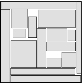
(a) Example of an orthogonal packing. All the packed rectangles are axis-parallel and non-overlapping.

(b) A non-orthogonal packing. With an orthogonal packing, only $4$ of the $5$ rectangles can be placed instead.

Figure 1.1: Orthogonal and non-orthogonal packings.

There is another interesting variant of these packing problem, where we are interested in packings that can be separated via the so called guillotine cuts, that is, edge-to-edge cuts parallel to an edge of the box. See Figure 1.2 for a comparison between a packing with guillotine cuts and a generic packing. Such constraints are common in scenarios where the packed rectangles are patches of a material that must be cut, where the availability of a guillotine cutting sequence simplify the cutting procedure, thereby reducing costs; see for example Puchinger et al. [2004] and Schneider [1988].

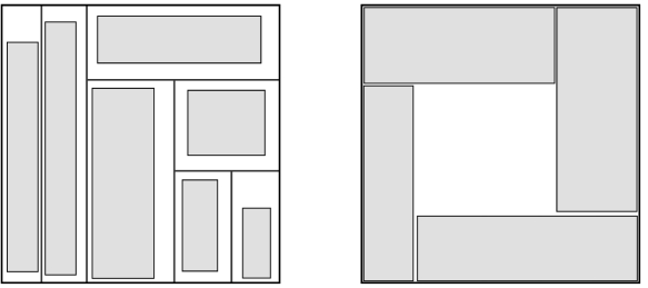
Figure 1.2: A guillotine packing on the left, and packing that cannot be a guillotine packing on the right.

1.4.1 Strip Packing

In the Strip Packing problem, we are given a parameter $W\in\mathbb{N}$ and a set ${\cal R}=\{R_{1},\ldots,R_{n}\}$ of $n$ rectangles, each one characterized by a positive integer width $w_{i}\in\mathbb{N}$, $w_{i}\leq W$, and a positive integer height $h_{i}\in\mathbb{N}$. Our goal is to find a value $h$ and a feasible packing of all the rectangles in $\mathcal{R}$ in a rectangle of size $W\times h$, while minimizing $h$.

The version with $90^{\circ}$ rotations is also considered.

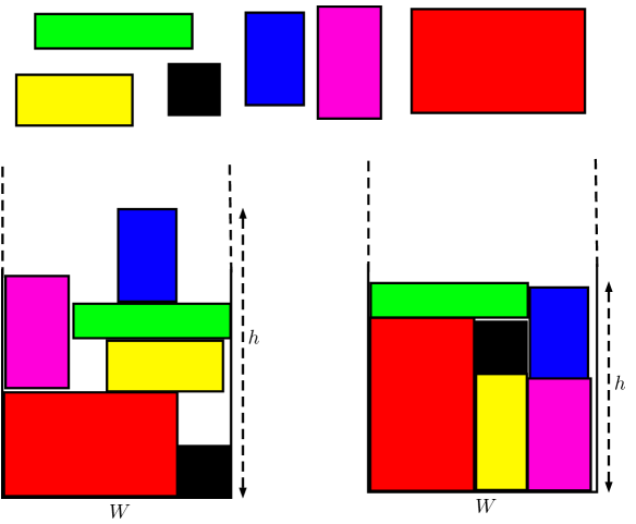
Figure 1.3: An instance of Strip Packing and corresponding feasible packings for the cases without (left) and with rotations (right).

Strip packing is a natural generalization of one-dimensional bin packing (obtained when all the rectangles have the same height; see Coffman Jr. et al. [2013]) and makespan minimization (obtained when all the rectangles have the same width; see Coffman and Bruno [1976]). The problem has lots of applications in industrial engineering and computer science, specially in cutting stock, logistics and scheduling (Kenyon and Rémila [2000]; Harren et al. [2014]). Recently, there have been several applications of strip packing in electricity allocation and peak demand reductions in smart-grids; see for example Tang et al. [2013], Karbasioun et al. [2013] and Ranjan et al. [2015].

A simple reduction from the Partition problem shows that the problem cannot be approximated within a factor $\frac{3}{2}-\varepsilon$ for any $\varepsilon>0$ in polynomial-time unless $\mathbf{P}=\mathbf{NP}$. This reduction relies on exponentially large (in $n$) rectangle widths, and it also applies for the case with rotations.

Let $OPT=OPT({\cal R})$ denote the optimal height for the considered strip packing instance $({\cal R},W)$, and $h_{\max}=h_{\max}({\cal R})$ (respectively, $w_{\max}=w_{\max}({\cal R})$) be the largest height (respectively, width) of any rectangle in ${\cal R}$. Most of the literature on this problem is devoted to the case without rotations. Observe that, for this case, $OPT\geq h_{\max}$, and we can assume that $W\leq nw_{\max}$ without loss of generality. The first non-trivial approximation algorithm for strip packing, with approximation ratio 3, was given by Baker et al. [1980]. The First-Fit-Decreasing-Height algorithm (FFDH) by Coffman Jr et al. [1980] gives a 2.7-approximation. Sleator [1980] gave an algorithm that generates a packing of height $2OPT+\frac{h_{max}}{2}$, hence achieving a 2.5-approximation. Afterwards, Steinberg [1997] and Schiermeyer [1994] independently improved the approximation ratio to 2. Harren and van Stee [2009] first broke the barrier of 2 with their 1.9396 approximation. The present best $(\frac{5}{3}+\varepsilon)$-approximation is due to Harren et al. [2014].

Nadiradze and Wiese [2016] overcame the $\frac{3}{2}$-inapproximability barrier by presenting a $(\frac{7}{5}+\epsilon)$-approximation algorithm running in pseudo-polynomial-time (PPT). More specifically, they provided an algorithm with running time $O((Nn)^{O(1)})$, where $N=\max\{w_{max},h_{max}\}$. In Gálvez, Grandoni, Ingala and Khan [2016], we improved the approximation factor to $4/3+\varepsilon$, also generalizing it to the case with $90^{\circ}$ rotations; this result is described in Chapter 3. For the case without rotations, an analogous result was independently obtained by Jansen and Rau [2017].

As strip packing is strongly NP-hard (see Garey and Johnson [1978]), it does not admit an exact pseudo-polynomial-time algorithm. Moreover, very recently Adamaszek et al. [2017] proved that it is $\mathbf{NP}$-hard to approximate Strip Packing within a factor $12/11-\varepsilon$ for any constant $\varepsilon>0$ in PPT, and this lower bound was further improved to $5/4-\varepsilon$ in Henning et al. [2017]. This rules out the possibility of a PPT approximation scheme.

The problem has been also studied in terms of asymptotic approximation, where the approximability is much better understood. For the case without rotations, Coffman Jr et al. [1980] analyzed two algorithms called Next Fit Decreasing Height (NFDH) and First Fit Decreasing Height (FFDH), and proved that their asymptotic approximation ratios are 2 and 1.7, respectively. Baker et al. [1980] described another heuristic called Bottom Leftmost Decreasing Width (BLWD), and proved that it is an asymptotic 2-approximation. Then Kenyon and Rémila [2000] provided an AFPTAS, that is, an asymptotic $(1+\varepsilon)$-approximation for any $\varepsilon>0$. The additive constant of $O\left(\frac{h_{max}}{\varepsilon^{2}}\right)$ was improved by Jansen and Solis-Oba [2009], who achieved an AFPTAS with additive constant only $h_{max}$. Sviridenko [2012] obtained a polynomial time algorithm that returns a solution with height at most $OPT+O(\sqrt{OPT\log OPT})$.

The analysis for the asymptotic 2-approximations (for example by NFDH) also apply to the case with $90^{\circ}$ rotations. Miyazawa and Wakabayashi [2004] improved this to a 1.613-approximation, and then Epstein and van Stee [2004b] proved a 1.5-approximation. Finally, Jansen and van Stee [2005] obtained an AFPTAS also for this variation of the problem.

The natural generalization of Strip Packing in 3 dimensions has been considered for the first time by Li and Cheng [1990], who obtained an asymptotic $3.25$-approximation. In Li and Cheng [1992], they further improved it to an asymptotic ratio $T_{\infty}^{2}\approx 2.89$, where $T_{\infty}\approx 1.69$ is the so called harmonic constant in the context of bin packing. Bansal et al. [2007] provided an asymptotic $T_{\infty}$-approximation. More recently, Jansen and Prädel [2014] obtained the currently best known asymptotic $1.5$-approximation. In terms of absolute approximation, the above mentioned result of Li and Cheng [1990] also implies a $45/4$-approximation, which was improved to $25/4$ in Diedrich et al. [2008].

1.4.2 2-Dimensional Geometric Knapsack

2-Dimensional Geometric Knapsack (2DGK) is a geometric generalization of the well studied one-dimensional knapsack problem. We are given a set of rectangles $\mathcal{R}=\{R_{1},\ldots,R_{n}\}$, where each $R_{i}$ is an axis-parallel rectangle with an integer width $w_{i}>0$, height $h_{i}>0$ and profit $p_{i}>0$, and a knapsack that we assume to be a square of size $N\times N$ for some integer $N>0$.

A feasible solution is any axis-aligned packing of a subset $\mathcal{R}^{\prime}\subseteq\mathcal{R}$ into the knapsack, and the goal is to maximize the profit $p(\mathcal{R}^{\prime})=\sum_{R_{i}\in\mathcal{R}^{\prime}}p_{i}$.

Like for Strip Packing, the variant with rotations of the problem is also considered, where one is allowed to rotate the rectangles by $90^{\circ}$.

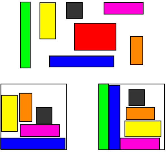
Figure 1.4: An instance of 2-Dimensional Geometric Knapsack, and corresponding feasible packing without (left) and with rotations (right); for simplicity, rectangle profits are not represented. Note that, unlike Strip Packing, it is not required that all the rectangles are packed.

The problem is motivated by several practical applications. For instance, one might want to place advertisements on a board or a website, or cut rectangular pieces from a sheet of some material (in this context, the variant with rotations is useful when the material does not have a texture, or the texture itself is rotation invariant). It can also model a scheduling setting where each rectangle corresponds to a job that needs some “contiguous amount” of a given resource (memory storage, frequencies, etc.). In all these cases, dealing only with rectangular shapes is a reasonable simplification.

Caprara and Monaci [2004] gave the first non-trivial approximation for the problem, obtaining ratio $3+\varepsilon$; this result builds on the $2$-approximation for Strip Packing in Steinberg [1997]. Jansen and Zhang [2007] obtained an algorithm with approximation factor $2+\varepsilon$, which is currently the best known in polynomial time; in Jansen and Zhang [2004] they also gave a simpler and faster $(2+\varepsilon)$-approximation for the special case in which all the rectangles have profit $1$ (cardinality case).

On the other hand, the only known hardness was given in Leung et al. [1990], who proved that an FPTAS is impossible even in the special case of packing squares into a square. Note that this does not rule out a PTAS.

Better results are known for many special cases. If all the rectangles are squares, Harren [2006] obtained a $(5/4+\varepsilon)$-approximation, and Jansen and Solis-Oba [2008] showed that a PTAS is possible; very recently, Heydrich and Wiese [2017] obtained an EPTAS. Fishkin et al. [2008] gave a PTAS for rectangles in the relaxed model with resource augmentation, that is, where one is allowed to enlarge the width and the height of the knapsack by a $1+\varepsilon$ factor. Jansen and Solis-Oba [2009] showed that the same can be achieved even if only the width (or only the height) is augmented; we prove a slightly modified version of this result in Lemma 14 in Section 2.5. Bansal, Caprara, Jansen, Prädel and Sviridenko [2009] proved that a PTAS is possible for the special case in which the profit of each rectangle equals its area, that is, $p_{i}:=w_{i}h_{i}$, for both the cases with or without rotations. Fishkin et al. [2005] presented a PTAS for the special case where the height of all the rectangles is much smaller than the height of the knapsack.

By using a structural result for independent set of rectangles, Adamaszek and Wiese [2015] gave a QPTAS for the case without rotations, with the assumption that widths and heights are quasi-polynomially bounded. Abed et al. [2015] extended the technique to obtain a similar QPTAS for the version with guillotine cuts (with the same assumption on rectangle sizes).

In Chapter 4 we show how to obtain a polynomial-time algorithm with approximation factor $17/9+\varepsilon$ for the case without rotations, which we further improve to $\frac{558}{325}+\varepsilon<1.72$ for the cardinality case. This is the first polynomial time algorithm that breaks the barrier of $2$ for this problem.

In Chapter 5 we consider the case with rotations, and obtain a $(3/2+\varepsilon)$-approximation for the general case, and a $(4/3+\varepsilon)$-approximation for the cardinality case.

The results in Chapters 4 and 5 are published in Gálvez, Grandoni, Heydrich, Ingala, Khan and Wiese [2017].

1.4.3 Related packing problems

Maximum Weight Independent Set of Rectangles (MWISR)

is the restriction of the well known Independent Set problem to the intersection graphs of 2D rectangles. We are given a set $\mathcal{R}$ of axis-aligned rectangles as above, but this time the coordinates $x_{i},y_{i}$ of the bottom-left corner of each rectangle $R_{i}$ are given as part of the input. The goal is to select a subset of rectangles $\mathcal{R}^{\prime}\subseteq\mathcal{R}$ of pairwise non-overlapping rectangles, while maximizing the total profit $p(\mathcal{R}^{\prime})=\sum_{R_{i}\in\mathcal{R}}p_{j}$ of the selected rectangles.

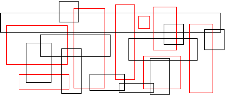
Figure 1.5: An instance of the Independent Set of Rectangles problem. Since the red rectangles are pairwise non-overlapping, they are a feasible solution to the problem.

While the Independent Set problem on general graphs is hard to approximate to $n^{1-\varepsilon}$ for any fixed $\varepsilon>0$, much better results are known for MWISR.

The best known approximation for general rectangles was given by Chan and Har-Peled [2012] and has ratio $O\left(\frac{\log n}{\log\log n}\right)$, slightly improving several previous $O(\log n)$-approximations (Agarwal et al. [1998]; Berman et al. [2001]; Chan [2004]). More recently, a breakthrough by Adamaszek and Wiese [2013] showed that a QPTAS is possible. Since only NP-hardness is known as a lower bound, this could suggest that a PTAS is possible for this problem, despite even a constant factor approximation is still not known.

Better results are known for many special cases of the problem. For the unweighted case, Chalermsook and Chuzhoy [2009] obtained a $(\log\log n)$-approximation. A PTAS is known for the special case when all the rectangles are squares (Erlebach et al. [2001]). Adamaszek et al. [2015] gave a PTAS for the relaxation of the problem when rectangles are allowed to be slightly shrunk (more precisely, each rectangle is rescaled by a factor $1-\delta$ for an arbitrarily small $\delta>0$).

In Chapter 6, we consider a generalization of MWISR where the input rectangles are partitioned into disjoint classes (bags), and only one rectangle per class is allowed in a feasible solution.

Storage Allocation Problem (SAP)

is a problem that arises in the context of resource allocation, but it still has a geometric nature. This problem is similar to 2DGK, with two important modifications:

• the horizontal position of each rectangle is fixed and given as part of the input (that is, the rectangle is only allowed to be moved vertically);

• the target region where each selected rectangle must be packed is the set of points in the positive quadrant that are below a given positive capacity curve $c(\cdot)$.

See Figure 1.6 for an example. This problems models the allocation of a resource that has a contiguous range and that varies over time, like bandwidth or disk allocation. Each rectangle represents a request to use the resource, starting at some specified time (the starting $x$-coordinate of the rectangle) and for a duration equal to the width of the rectangle. The height of the rectangle represents the amount of the resource that is requested.

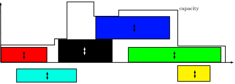
Figure 1.6: An instance and a feasible solution of the Storage Allocation Problem; two rectangles are not packed. Selected rectangles can only be moved vertically.

Bar-Yehuda et al. [2013] gave the first constant factor approximation for this problem, with ratio $9+\varepsilon$; the best known result, with approximation factor $2+\varepsilon$, is due to Mömke and Wiese [2015].

See Chapter 6 for more related scheduling problems.

2$-DimensionalGeometricBinPacking$

is another important geometric packing problem, generalizing the well studied bin packing problem, which is its $1$-dimensional counterpart. Here, we are given an instance as in 2DGK, but we want to pack all the given rectangles in square knapsacks of size $N\times N$; our goal is to minimize the number of knapsacks used. As for the other problems, both the variants with or without $90^{\circ}$ rotations are considered.

There is an extensive literature regarding asymptotic approximation algorithms. The first results were obtained by Chung et al. [1982], who provided a $2.125$-approximation. The approximation ratio was improved to $(2+\varepsilon)$ in Kenyon and Rémila [2000], and then further reduced to $T_{\infty}+\varepsilon$ by Caprara [2002], where $T_{\infty}\approx 1.691...$ is the so-called harmonic constant. Bansal, Caprara and Sviridenko [2009] improved the approximation ratio to $1+\ln T_{\infty}\approx 1.52$, using a general framework known as Round-and-Approx. Then, Jansen and Prädel [2013] obtained a $1.5$-approximation, which was improved to $1+\ln 1.5\approx 1.405$ by Bansal and Khan [2014] with the Round-and-Approx framework. Bansal, Correa, Kenyon and Sviridenko [2006] proved that an asymptotic PTAS is impossible, unless $\mathbf{P}=\mathbf{NP}$; Chlebík and Chlebíková [2006] extended this result to the case with rotations, and also proved explicit lower bounds, showing that it is impossible to approximate $2$-Dimensional Geometric Bin Packing with an asymptotic ratio smaller than $1+1/3792$ for the version without rotations, and smaller than $1+1/2196$, for the versions with rotations.

For the special case of squares, Fereira et al. [1998] obtained a $1.998$-approximation, which was improved to a $(14/9+\varepsilon)$-approximation by Kohayakawa et al. [2004] and Seiden and van Stee [2002]. An algorithm analyzed by Caprara [2002] is shown to have an approximation ratio between $1.490$ and $1.507$, although the proof conditionally depends on a certain conjecture. Epstein and van Stee [2004a] obtained a $(16/11+\varepsilon)$-approximation. Bansal, Correa, Kenyon and Sviridenko [2006] proved that an APTAS is possible for squares (and, more generally, for the $d$-dimensional generalization of the problem). They gave an exact algorithm for the relaxation of the problem on rectangles with resource augmentation, that is, where the bins are augmented by a factor $1+\varepsilon$. Moreover, they provided a PTAS on the related problem of placing a set of rectangles in a minimum-area enclosing rectangle.

Fewer results ar known regarding absolute approximations. As shown by Leung et al. [1990], even if the problem is restricted to squares, it is $\mathbf{NP}$-hard to distinguish if $1$ or $2$ bins are needed. Zhang [2005] obtained a $3$-approximation for the case without rotations, and van Stee [2004] showed that a $2$-approximation is possible for the case of squares. Then, Harren and van Stee [2012] showed that a $2$-approximation is possible for general rectangles if rotations are allowed. Note that, due to the $\mathbf{NP}$-hardness mentioned above, an absolute ratio of $2$ is the best possible for any of these problems.

Bansal et al. [2005] proved the surprising result that an asymptotic PTAS is possible for the version of the problem with guillotine cuts.

Many results are also known in the online version of the above problems; we omit them here. A recent review of these and other related problems can be found in Christensen et al. [2017].

1.5 Summary of our results and outline of this thesis

In Chapter 2, we review some preliminary results and develop some useful tools for rectangle packing problems.

Many results in this area of research are obtained by showing that a profitable solution exists that presents a special, simplified structure: namely, the target area where the rectangles are packed is partitioned into a constant number of rectangular regions, whose sizes are chosen from a polynomial set of possibilities. Thus, such simplified structures can be guessed efficiently, and then used to guide the subsequent rectangle selection and packing procedure.

Following the same general approach, we will define one such special structure that we call container packings, which we define in Section 2.4. Then, in Sections 2.3 and 2.4.1 we show that there is a relatively simple PTAS for container packings based on Dynamic Programming. Notably, this PTAS does not require the solution of any linear program and is purely combinatorial, and it is straightforward to adapt it to the case with $90^{\circ}$ rotations.

Container packings are a valuable black box tool for rectangle packing problems, generalizing several other such simplified structures used in literature. In Section 2.5 we reprove a known result on 2DGK with Resource Augmentation in terms of container packings. We use this modified version in several of our results.

In Chapter 3, we present our new $(4/3+\varepsilon)$-approximation for Strip Packing in pseudo-polynomial time. The results of this chapter are based on Gálvez, Grandoni, Ingala and Khan [2016], published at the 36th IARCS Annual Conference on Foundations of Software Technology and Theoretical Computer Science, December 13–15 2016, Chennai, India. This result improves on the previously best known $(1.4+\varepsilon)$-approximation by Nadiradze and Wiese [2016] with a novel repacking lemma which is described in Section 3.2. Moreover by using container packings, we obtain a purely combinatorial algorithm (that is, no linear program needs to be solved), and we can easily adapt the algorithm to the case with $90^{\circ}$ rotations.

Chapters 4 and 5 present our results on 2DGK and 2DGKR from Gálvez, Grandoni, Heydrich, Ingala, Khan and Wiese [2017], published at the 58th Annual IEEE Symposium on Foundations of Computer Science, October 15–17 2017, Berkeley, California.

In Chapter 4, we present the first polynomial time approximation algorithm that breaks the barrier of $2$ for the 2DGK problem (without rotations). Although we still use container packings, a key factor in this result is a PTAS for another special packing problem that we call L-packing, which does not seem to be possible to solve with a purely container-based approach. Combining this PTAS with container packing will yield our main result, which is an algorithm with approximation ratio $\frac{17}{9}+\varepsilon<1.89$. For the unweighted case, we can further refine the approximation ratio to $\frac{558}{325}+\varepsilon<1.717$ by means of a quite involved case analysis.

In Chapter 5, we focus on 2DGKR, and we show a relatively simple polynomial time $(3/2+\varepsilon)$-approximation for the general case; for the unweighted case, we improve it to $4/3+\varepsilon$ in Section 5.2. In this case, we do not need L-packings, and we again use a purely container-based approach.

In Chapter 6, we study a generalization of the MWISR problem that we call bagMWISR, and we use it to obtain improved approximation for a scheduling problem called bagUFP. A preliminary version of these results was contained in Grandoni, Ingala and Uniyal [2015], published in the 13th Workshop on Approximation and Online Algorithms, September 14–18 2015, Patras, Greece. In Section 6.3 we show that we can generalize the $\left(\frac{\log\log n}{\log n}\right)$-approximation for MWISR by Chan and Har-Peled [2012], which is based on the randomized rounding with alterations framework, to the more general bagMWISR problem, obtaining in turn an improved approximation ratio for bagUFP. Then, in Section 6.4, we turn our attention to the unweighted case of bagUFP, and we show that the special instances of bagMWISR that are generated by the reduction from bagUFP have a special structure that can be used to obtain a $O(1)$-approximation. This result builds on the work of Anagnostopoulos et al. [2014].

Chapter 2 Preliminaries

In this chapter, we introduce some important tools and preliminary results that we will use extensively in the following chapters. Some results are already mentioned in literature, and we briefly review them; some others, while they are not published in literature to the best of our knowledge, are based on standard techniques; since they are crucial to our approaches, we provide full proofs of them.

2.1 Next Fit Decreasing Height

One of the most recurring tools used as a subroutine in countless results on geometric packing problems is the Next Fit Decreasing Height (NFDH) algorithm, which was originally analyzed in Coffman Jr et al. [1980] in the context of Strip Packing. We will use a variant of this algorithm to pack rectangles inside a box.

Suppose you are given a box $C$ of size $w\times h$, and a set of rectangles $I^{\prime}$ each one fitting in the box (without rotations). NFDH computes in polynomial time a packing (without rotations) of $I^{\prime\prime}\subseteq I^{\prime}$ as follows. It sorts the rectangles $i\in I^{\prime}$ in non-increasing order of height $h_{i}$, and considers rectangles in that order $i_{1},\ldots,i_{n}$. Then the algorithm works in rounds $j\geq 1$. At the beginning of round $j$ it is given an index $n(j)$ and a horizontal segment $L(j)$ going from the left to the right side of $C$. Initially $n(1)=1$ and $L(1)$ is the bottom side of $C$. In round $j$ the algorithm packs a maximal set of rectangles $i_{n(j)},\ldots,i_{n(j+1)-1}$, with bottom side touching $L(j)$ one next to the other from left to right (a shelf). The segment $L(j+1)$ is the horizontal segment containing the top side of $i_{n(j)}$ and ranging from the left to the right side of $C$. The process halts at round $r$ when either all the rectangles have being packed or $i_{n(r+1)}$ does not fit above $i_{n(r)}$. See Figure 2.1 for an example of packing produced by this algorithm.

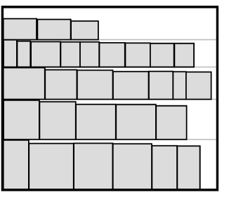
Figure 2.1: A packing obtained using the classical Next Fit Decreasing Height algorithm.

We prove the following known result:

Lemma 1.

Let $C$ be a given box of size $w\times h$, and let $I^{\prime}$ be a set of rectangles. Assume that, for some given parameter $\varepsilon\in(0,1)$, for each $i\in I^{\prime}$ one has $w_{i}\leq\varepsilon w$ and $h_{i}\leq\varepsilon h$. Then NFDH is able to pack in $C$ a subset $I^{\prime\prime}\subseteq I^{\prime}$ of total area at least $a(I^{\prime\prime})\geq\min\{a(I^{\prime}),(1-2\varepsilon)w\cdot h\}$. In particular, if $a(I^{\prime})\leq(1-2\varepsilon)w\cdot h$, all the rectangles in $I^{\prime}$ are packed.

Proof.

The claim trivially holds if all rectangles are packed. Thus suppose that this is not the case. Observe that $\sum_{j=1}^{r+1}h_{i_{n(j)}}>h$, otherwise the rectangle $i_{n(r+1)}$ would fit in the next shelf above $i_{n(r)}$; hence $\sum_{i=2}^{r+1}h_{i_{n(j)}}>h-h_{i_{n(1)}}\geq(1-\varepsilon)h$. Observe also that the total width of the rectangles packed in each round $j$ is at least $w-\varepsilon w=(1-\varepsilon)w$, since $i_{n(j+1)}$, of width at most $\varepsilon w$, does not fit to the right of $i_{n(j+1)-1}$. It follows that the total area of the rectangles packed in round $j$ is at least $(w-\varepsilon w)h_{n(j+1)-1}$, and thus:

$$a(I^{\prime\prime})\geq\sum_{j=1}^{r}(1-\varepsilon)w\cdot h_{n(j+1)-1}\geq(1-\varepsilon)w\sum_{j=2}^{r+1}h_{n(j)}\geq(1-\varepsilon)^{2}w\cdot h\geq(1-2\varepsilon)w\cdot h.$$

∎

We can use NFDH as an algorithm for Strip Packing, where we work on a box of fixed with $W$ and unbounded height, and we pack all elements. In this context, the following result holds:

Lemma 2 (Coffman Jr et al. [1980]).

Given a strip packing instance $(\mathcal{R},W)$, the NFDH algorithm gives a packing of height at most $h_{\max}(\mathcal{R})+\frac{2a(\mathcal{R})}{W}$.

2.2 Steinberg’s algorithm

The following theorem gives sufficient conditions to pack a given set of rectangles in a rectangular box. We denote $x_{+}:=\max(x,0)$.

Theorem 3 (Steinberg [1997]).

Suppose that we are given a set of rectangles $I^{\prime}$ and a box $Q$ of size $w\times h$. Let $w_{max}\leq w$ and $h_{max}\leq h$ be the maximum width and maximum height among the rectangles in $I^{\prime}$ respectively. If

$$2a(I^{\prime})\leq wh-(2w_{max}-w)_{+}(2h_{max}-h)_{+}$$

then all the rectangles in $I^{\prime}$ can be packed into $Q$ in polynomial time.

In particular, we will use the following simpler corollary:

Corollary 4.

Suppose that we are given a set of rectangles $I^{\prime}$ and a box $Q$ of size $w\times h$. Moreover, suppose that each rectangle in $I^{\prime}$ has width at most $w/2$ (resp. each rectangle in $I^{\prime}$ has height at most $h/2$), and $a(I^{\prime})\leq wh/2$. Then all the rectangles in $I^{\prime}$ can be packed into $Q$ in polynomial time.

2.3 The Maximum Generalized Assignment Problem

In this section we show that there is a PTAS for the Maximum Generalized Assignment Problem (GAP) if the number of bins is constant.

GAP is a powerful generalization of the Knapsack problem. We are given a set of $k$ bins, where bin $j$ has capacity $c_{j}$, and a set of $n$ items. Let us assume that if item $i$ is packed in bin $j$, then it requires size $s_{ij}\in\mathbb{Z}$ and has profit $p_{ij}\in\mathbb{Z}$. Our goal is to select a maximum profit subset of items, while respecting the capacity constraints on each bin.

GAP is known to be APX-hard and the best known polynomial time approximation algorithm has ratio $(1-1/e+\varepsilon)$ (Fleischer et al. [2011]; Feige and Vondrak [2006]). In fact, for an arbitrarily small constant $\delta>0$ (which can even be a function of $n$) GAP remains APX-hard even on the following very restricted instances: bin capacities are identical, and for each item $i$ and bin $j$, $p_{ij}=1$, and $s_{ij}=1$ or $s_{ij}=1+\delta$ (Chekuri and Khanna [2005]). The complementary case, where item sizes do not vary across bins but profits do, is also APX-hard. However, when all profits and sizes are the same across all the bins (that is, $p_{ij}=p_{ik}$ and $s_{ij}=s_{ik}$ for all bins $j,k$), the problem is known as multiple knapsack problem (MKP) and it admits a PTAS.

Let $p(OPT)$ be the cost of the optimal assignment. First, we show that we can solve GAP exactly in pseudopolynomial time.

Lemma 5.

There is an algorithm running in time $O\left(nD^{k}\right)$ that finds an optimal solution for the maximum generalized assignment problem, where there are $k$ bins and each of them has capacity at most $D$.

Proof.

For each $i\in[n]$ and $d_{j}\in[c_{j}]$ for $j\in[k]$, let $S_{i,d_{1},d_{2},\dots,d_{k}}$ denote a subset of the set of items $\{1,2,\dots,i\}$ packed into the bins such that the profit is maximized and the capacity of bin $j$ is at most $d_{j}$. Let $P[i,d_{1},d_{2},\dots,d_{k}]$ denote the profit of $S_{i,d_{1},d_{2},\dots,d_{k}}$. Clearly $P[1,d_{1},d_{2},\dots,d_{k}]$ is known for all $d_{j}\in[c_{j}]$ for $j\in[k]$. Moreover, for convenience we define $P[i,d_{1},d_{2},\dots,d_{k}]=0$ if $d_{j}<0$ for any $j\in[k]$. We can compute the value of $P[i,d_{1},d_{2},\dots,d_{k}]$ by using a dynamic program (DP), that exploits the following recurrence:

$$P[i,d_{1},d_{2},\dots,d_{k}]=\max\{ P[i-1,d_{1},d_{2},\dots,d_{k}],$$

$$\max_{j}\{p_{ij}+P[i-1,d_{1},\dots,d_{j}-s_{ij},\dots,d_{k}]\}\}$$

With a similar recurrence, we can easily compute a corresponding set $S_{i,d_{1},d_{2},\dots,d_{k}}$.
Clearly, this dynamic program can be executed in time $O\Big{(}n\prod\limits_{j=1}^{k}c_{j}\Big{)}=O\left(nD^{k}\right)$. ∎

The following lemma shows that we can also solve GAP optimally even in polynomial time, if we are allowed a slight violation of the capacity constraints (that is, in the resource augmentation model).

Lemma 6.

There is a $O\left({\left(\frac{1+\varepsilon}{\varepsilon}\right)}^{k}n^{k+1}\right)$ time algorithm for the maximum generalized assignment problem with $k$ bins, which returns a solution with profit at least $p(OPT)$ if we are allowed to augment the bin capacities by a $(1+\varepsilon)$-factor for any fixed $\varepsilon>0$.

Proof.

In order to obtain a polynomial time algorithm from Lemma 5, we want to construct a modified instance where each capacity $c_{j}$ is polynomially bounded.

For each bin $j$, let $\mu_{j}=\frac{\varepsilon c_{j}}{n}$. For item $i$ and bin $j$, define the modified size $s^{\prime}_{ij}=\left\lceil\frac{s_{ij}}{\mu_{j}}\right\rceil=\left\lceil\frac{ns_{ij}}{\varepsilon c_{j}}\right\rceil$ and $c^{\prime}_{j}=\left\lfloor\frac{(1+\varepsilon)c_{j}}{\mu_{j}}\right\rfloor$. Note that $c^{\prime}_{j}=\left\lfloor\frac{(1+\varepsilon)n}{\varepsilon}\right\rfloor\leq\frac{(1+\varepsilon)n}{\varepsilon}$, so the algorithm from Lemma 5 requires time at most $O\left(n\cdot\left(\frac{(1+\varepsilon)n}{\varepsilon}\right)^{k}\right)$.

Let $OPT_{modified}$ be the solution found for the modified instance. Now consider the optimal solution for the original instance (that is, with the original item and bin sizes) $OPT$. If we show that the same assignment of items to the bins is a feasible solution (with modified bin sizes and item sizes) for the modified instance, we obtain that $p(OPT_{modified})\geq p(OPT)$ and that will conclude the proof.

Let $S_{j}$ be the set of items packed in bin $j$ in $OPT$. Since it is feasible, we have that $\sum_{i\in S_{j}}s_{ij}\leq c_{j}$. Hence,

$$\sum_{i\in S_{j}}s^{\prime}_{ij} \leq\left\lfloor\sum_{i\in S_{j}}\left(\frac{s_{ij}}{\mu_{j}}+1\right)\right\rfloor\leq\left\lfloor\frac{1}{\mu_{j}}\left(\sum_{i\in S_{j}}s_{ij}+|S_{j}|\mu_{j}\right)\right\rfloor$$

$$\leq\left\lfloor\frac{1}{\mu_{j}}(c_{j}+n\mu_{j})\right\rfloor=\left\lfloor\frac{(1+\varepsilon)c_{j}}{\mu_{j}}\right\rfloor=c^{\prime}_{j}$$

Thus $OPT$ is a feasible solution for the modified instance and the above algorithm will return a packing with profit at least $p(OPT)$ under $\varepsilon$-resource augmentation. ∎

Now we can show how to employ this result to obtain a PTAS for GAP without violating the bin capacities. We first prove the following technical lemma.

Lemma 7.

If a set of items $R_{j}$ is packed in a bin $j$ with capacity $c_{j}$, then there exists a set of at most $1/\varepsilon^{2}$ items $X_{j}$, and a set of items $Y_{j}$ with $p(Y_{j})\leq\varepsilon p(R_{j})$ such that all items in $R_{j}\setminus(X_{j}\cup Y_{j})$ have size at most $\varepsilon(c_{j}-\sum_{i\in X_{j}}s_{ij})$.

Proof.

Let $Q_{1}$ be the set of items $i$ with $s_{ij}>\varepsilon c_{j}$. If $p(Q_{1})\leq\varepsilon p(R_{j})$, we are done by taking $Y_{j}=Q_{1}$ and $X_{j}=\phi$. Otherwise, define $X_{j}:=Q_{1}$ and we continue the next iteration with the remaining items. Let $Q_{2}$ be the items with size greater than $\varepsilon(c_{j}-\sum_{i\in X_{j}}s_{ij})$ in $R_{j}\setminus X_{j}$. If $p(Q_{2})\leq\varepsilon p(R_{j})$, we are done by taking $Y_{j}=Q_{2}$. Otherwise define $X_{j}:=Q_{1}\cup Q_{2}$ and we continue with further iterations till we get a set $Q_{t}$ with $p(Q_{t})\leq\varepsilon p(R_{j})$. Note that we need at most $\frac{1}{\varepsilon}$ iterations, since the sets $Q_{i}$ are disjoint. Otherwise:

$$p(R_{j})\geq\sum\limits_{i=1}^{1/\varepsilon}p(Q_{i})>\sum\limits_{i=1}^{1/\varepsilon}\varepsilon p(R_{j})\geq p(R_{j})$$

which is a contradiction. Thus, consider $Y_{j}=Q_{t}$ and $X_{j}=\bigcup_{l=1}^{t-1}Q_{l}$. One has $|X_{j}|\leq 1/\varepsilon^{2}$ and $p(Y_{j})\leq\varepsilon p(R_{j})$. On the other hand, after removing $Q_{t}$, the remaining items have size smaller than $\varepsilon(c_{j}-\sum_{i\in X_{j}}s_{ij})$. ∎

Lemma 8.

There is an algorithm for the maximum generalized assignment problem with $k$ bins that runs in time $O\left(\left(\frac{1+\varepsilon}{\varepsilon}\right)^{k}n^{k/\varepsilon^{2}+k+1}\right)$ and returns a solution that has profit at least $(1-3\varepsilon)p(OPT)$, for any fixed $\varepsilon>0$.

Proof.

Consider a bin $j$ that contains the set $R_{j}$ of items in the optimal solution OPT, and let $X_{j}$ and $Y_{j}$ the sets given by Lemma 7. Let $c^{\prime}_{j}=c_{j}-\sum_{i\in X_{j}}s_{ij}$ be the residual capacity, so that each element in the set $R^{\prime}_{j}:=R_{j}\setminus(X_{j}\cup Y_{j})$ has size in $j$ smaller than $\varepsilon c^{\prime}_{j}$. We divide the residual space into $1/\varepsilon$ equally sized intervals $S_{j,1},S_{j,2},\dots,S_{j,{1/\varepsilon}}$ of lengths $\varepsilon c^{\prime}_{j}$. Let $R^{\prime}_{j,l}$ be the set of items intersecting the interval $S_{j,l}$. As each packed item can belong to at most two such intervals, the cheapest set $R^{\prime\prime}$ among $\{R^{\prime}_{j,1},\dots,R^{\prime}_{j,1/\varepsilon}\}$ has profit at most $2\varepsilon p(R^{\prime}_{j})$. Thus we can remove this set $R^{\prime\prime}$ and reduce the bin size by a factor of $(1-\varepsilon)$.

Now consider the packing of the $k$ bins in the optimal packing $OPT$. Let $R_{j}$ be the set of items packed in bin $j$.

The algorithm first guesses all $X_{j}$’s, a constant number of items, in all $k$ bins. We assign them to corresponding bins, implying a $O(n^{k/\varepsilon^{2}})$ factor in the running time. Then for bin $j$ we are left with capacity $c^{\prime}_{j}$. From the previous discussion, we know that there is packing of $R^{\prime\prime}_{j}\subseteq R_{j}\setminus X_{j}$ of profit $(1-2\varepsilon)p(R_{j}\setminus X_{j})$ in a bin with capacity $(1-\varepsilon)c^{\prime}_{j}$. Thus we can use the algorithm for GAP with resource augmentation provided by Lemma 6 to pack the remaining items in $k$ bins where for bin $j$ we use the original capacity to be $(1-\varepsilon)c^{\prime}_{j}$ for $j\in[k]$; note that $(1-\varepsilon)(1+\varepsilon)\leq 1$, so the solution is feasible with the capacities $c^{\prime}_{j}$. As Lemma 6 returns the optimal packing on this modified bin sizes, we obtain a total profit of at least $(1-2\varepsilon)(1-\varepsilon)p(OPT)\geq(1-3\varepsilon)p(OPT)$. The running time is the same as in Lemma 6 multiplied by the $O(n^{k/\varepsilon^{2}})$ factor for the initial item guessing and assignment. ∎

2.4 Container packings

In this section we define the main concept of our framework: a container.

Many of the literature results on geometric packing problems follow (implicitly or explicitly) the following approach: since the number of possible packings is too big to be enumerated, a search algorithm is performed only on a restricted family of packings that have a special structure. Thus, the theoretical analysis aims to prove that there exists such a restricted packing that has a high profit.

We follow the same general framework, by defining what we call a container packing.

By container we mean a special kind of box to which we assign a set of rectangles that satisfy some constraints, as follows (see Figure 2.2):

• A horizontal container is a box such that any horizontal line overlaps at most one rectangle packed in it.

• A vertical container is a box such that any vertical line overlaps at most one rectangle packed in it.

• An $\varepsilon$-granular area container is a box, say of size $w\times h$, such that all the rectangles that are packed inside have width at most $\varepsilon w$ and height at most $\varepsilon h$. We will simply talk about an area container when the value of $\varepsilon$ is clear from the context.

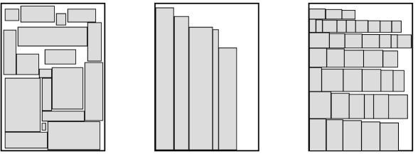
Figure 2.2: From left to right: a box, which is a rectangular region with arbitrary rectangles packed inside; a vertical container, which is a box where rectangles are piled from left to right; an area container, where width and height of the rectangles inside is much smaller than the width and height of the container, making it easy to pack them by NFDH.

A packing such that all the packed rectangles are contained in a container and all the area containers are $\varepsilon$-granular is called and $\varepsilon$-granular container packing; again, we will simply call it a container packing when the choice of $\varepsilon$ is clear from the context.

Observe that for a horizontal or a vertical container, once a set of rectangles that can feasibly be packed is assigned, constructing a packing is trivial. Moreover, the next lemma shows that it is easy to pack almost all the rectangles assigned to an area container:

Lemma 9.

Suppose that a set $\mathcal{R}$ of rectangles is assigned to an $\varepsilon$-granular area container $C$, and $a(\mathcal{R})\leq a(C)$. Then it is possible to pack in $C$ a subset of $\mathcal{R}$ of profit at least $(1-3\varepsilon)p(\mathcal{R})$.

Proof.

If $a(\mathcal{R})\leq(1-2\varepsilon)a(C)$, then NFDH can pack all the rectangles by Lemma 1. Suppose that $a(\mathcal{R})>(1-2\varepsilon)a(C)$. Consider the elements of $\mathcal{R}$ by non-increasing order of profit over area ratio. Let $\mathcal{R^{\prime}}$ be the maximal subset of rectangles of $\mathcal{R}$ in the specified order such that $a(\mathcal{R}^{\prime})\leq(1-2\varepsilon)a(C)$. Since $a(R)\leq\varepsilon^{2}a(C)$ for each $R\in\mathcal{R}$, then $a(R^{\prime})\geq(1-2\varepsilon-\varepsilon^{2})a(C)\geq(1-3\varepsilon)a(C)$, and then $a(R^{\prime})\geq(1-3\varepsilon)a(R)$, which implies $p(\mathcal{R}^{\prime})\geq(1-3\varepsilon)p(\mathcal{R})$ by the choice of $R^{\prime}$. Since $a(\mathcal{R}^{\prime})\leq(1-2\varepsilon)a(C)$, then NFDH can pack all of $\mathcal{R}^{\prime}$ inside $C$ by Lemma 1. ∎

In the remaining part of this section, we show that container packings are easy to approximate if the number of containers is bounded by some fixed constant.

2.4.1 Rounding containers

In this subsection we show that it is possible to round down the size of a horizontal, vertical or area container so that the resulting sizes can be chosen from a polynomially sized set, while incurring in a negligible loss of profit.

We say that a container $C^{\prime}$ is smaller than a container $C$ if $w(C^{\prime})\leq w(C)$ and $h(C^{\prime})\leq h(C)$. Given a container $C$ and a positive $\varepsilon<1$, we say that a rectangle $R_{j}$ is $\varepsilon$-small for $C$ if $w_{j}\leq\varepsilon w(C)$ and $h_{j}\leq\varepsilon h(C)$.

For a set $\mathcal{R}$ of rectangles, we define $WIDTHS(\mathcal{R})=\{w_{j}\,|\,R_{j}\in\mathcal{R}\}$ and $HEIGHTS(R)=\{h_{j}\,|\,R_{j}\in\mathcal{R}\}$.

Given a finite set $P$ of real numbers and a fixed natural number $k$, we define the set $P^{(k)}=\{(p_{1}+p_{2}+\dots+p_{l})+ip_{l+1}\,|\,p_{j}\in P\text{ }\forall\,j,l\leq k,0\leq i\leq n,i\mbox{ integer}\}$; note that if $|P|=O(n)$, then $|P^{(k)}|=O(n^{k+2})$. Moreover, if $P\subseteq Q$, then obviously $P^{(k)}\subseteq Q^{(k)}$, and if $k^{\prime}\leq k^{\prime\prime}$, then $P^{(k^{\prime})}\subseteq P^{(k^{\prime\prime})}$.

Lemma 10.

Let $\varepsilon>0$, and let $\mathcal{R}$ be a set of rectangles packed in a horizontal or vertical container $C$. Then, for any $k\geq 1/\varepsilon$, there is a set $\mathcal{R}^{\prime}\subseteq\mathcal{R}$ with profit $p(\mathcal{R}^{\prime})\geq(1-\varepsilon)p(\mathcal{R})$ that can be packed in a container $C^{\prime}$ smaller than $C$ such that $w(C^{\prime})\in WIDTHS(\mathcal{R})^{(k)}$ and $h(C^{\prime})\in HEIGHTS(R)^{(k)}$.

Proof.

Without loss of generality, we prove the thesis for an horizontal container $C$; the proof for vertical containers is symmetric. Clearly, the width of $C$ can be reduced to $w_{max}(\mathcal{R})$, and $w_{max}(\mathcal{R})\in WIDTHS(\mathcal{R})\subseteq{WIDTHS(\mathcal{R})}^{(k)}$.

If $|\mathcal{R}|\leq 1/\varepsilon$, then $\sum_{R_{i}\in\mathcal{R}}h_{i}\in HEIGHTS(\mathcal{R})^{(k)}$ and there is no need to round the height of $C$ down. Otherwise, let $\mathcal{R}_{TALL}$ be the set of the $1/\varepsilon$ rectangles in $\mathcal{R}$ with largest height (breaking ties arbitrarily), let $R_{j}$ be the least profitable of them, and let $\mathcal{R}^{\prime}=\mathcal{R}\setminus\{R_{j}\}$. Clearly, $p(\mathcal{R}^{\prime})\geq(1-\varepsilon)p(\mathcal{R})$. Since each element of $\mathcal{R}^{\prime}\setminus\mathcal{R}_{TALL}$ has height at most $h_{j}$, it follows that $h(\mathcal{R}\setminus\mathcal{R}_{TALL})\leq(n-1/\varepsilon)h_{j}$. Thus, letting $i=\left\lceil h(\mathcal{R}^{\prime}\setminus\mathcal{R}_{TALL})/h_{j}\right\rceil\leq n$, all the rectangles in $\mathcal{R}^{\prime}$ fit in a container $C^{\prime}$ of width $w_{max}(\mathcal{R})$ and height $h(C^{\prime}):=h(\mathcal{R}_{TALL})+ih_{j}\in{HEIGHTS(R)}^{(k)}$. Since $h(\mathcal{R}_{TALL})+ih_{j}\leq h(\mathcal{R}_{TALL})+h(\mathcal{R}^{\prime}\setminus\mathcal{R}_{TALL})+h_{j}=h(\mathcal{R})\leq h(C)$, this proves the result. ∎

Lemma 11.

Let $\varepsilon>0$, and let $\mathcal{R}$ be a set of rectangles that are assigned to an area container $C$. Then there exists a subset $\mathcal{R}^{\prime}\subseteq\mathcal{R}$ with profit $p(\mathcal{R}^{\prime})\geq(1-3\varepsilon)p(\mathcal{R})$ and a container $C^{\prime}$ smaller than $C$ such that: $a(\mathcal{R}^{\prime})\leq a(C)$, $w(C^{\prime})\in{WIDTHS(\mathcal{R})}^{(0)}$, $h(C^{\prime})\in{HEIGHTS(\mathcal{R})}^{(0)}$, and each $R_{j}\in\mathcal{R}^{\prime}$ is $\dfrac{\varepsilon}{1-\varepsilon}$-small for $C^{\prime}$.

Proof.

Without loss of generality, we can assume that $w(C)\leq nw_{max}(\mathcal{R})$ and $h(C)\leq nh_{max}(\mathcal{R})$: if not, we can first shrink $C$ so that these conditions are satisfied, and all the rectangles still fit in $C$.

Define a container $C^{\prime}$ that has width $w(C^{\prime})=w_{max}(\mathcal{R})\left\lfloor w(C)/w_{max}(\mathcal{R})\right\rfloor$ and height $h(C^{\prime})=h_{max}(\mathcal{R})\left\lfloor h(C)/h_{max}(\mathcal{R})\right\rfloor$, that is, $C^{\prime}$ is obtained by shrinking $C$ to the closest integer multiples of $w_{max}(\mathcal{R})$ and $h_{max}(\mathcal{R})$. Observe that $w(C^{\prime})\in{WIDTHS(\mathcal{R})}^{(0)}$ and $h(C^{\prime})\in{HEIGHTS(\mathcal{R})}^{(0)}$. Clearly, $w(C^{\prime})\geq w(C)-w_{max}(\mathcal{R})\geq w(C)-\varepsilon w(C)=(1-\varepsilon)w(C)$, and similarly $h(C^{\prime})\geq(1-\varepsilon)h(C^{\prime})$. Hence $a(C^{\prime})\geq(1-\varepsilon)^{2}a(C)\geq(1-2\varepsilon)a(C)$.

We now select a set $\mathcal{R}^{\prime}\subseteq\mathcal{R}$ by greedily choosing elements from $\mathcal{R}$ in non-increasing order of profit/area ratio, adding as many elements as possible without exceeding a total area of $(1-2\varepsilon)a(C)$. Since each element of $\mathcal{R}$ has area at most $\varepsilon^{2}a(C)$, then either all elements are selected (and then $p(\mathcal{R}^{\prime})=p(\mathcal{R})$), or the total area of the selected elements is at least $(1-2\varepsilon-\varepsilon^{2})a(C)\geq(1-3\varepsilon)a(C)$. By the greedy choice, we have that $p(\mathcal{R}^{\prime})\geq(1-3\varepsilon)p(\mathcal{R})$.

Since each rectangle in $\mathcal{R}$ is $\frac{\varepsilon}{1-\varepsilon}$-small for $C^{\prime}$, this proves the thesis. ∎

Remark.

Note that in the above, the size of the container is rounded to a family of sizes that depends on the rectangles inside; of course, they are not known in advance in an algorithm that enumerates over all the container packings. On the other hand, if the instance is a set $\mathcal{\mathcal{I}}$ of $n$ rectangles, then for any fixed natural number $k$ we have that $WIDTHS(\mathcal{R})^{(k)}\subseteq WIDTHS(\mathcal{I})^{(k)}$ and $HEIGHTS(\mathcal{R})^{(k)}\subseteq WIDTHS(\mathcal{\mathcal{I}})^{(k)}$ for any $\mathcal{R}\subseteq\mathcal{I}$; clearly, the resulting set of possible widths and heights has a polynomial size and can be computed from the input.

Similarly, when finding container packings for the case with rotations, one can compute the set $SIZES(\mathcal{I}):=WIDTHS(\mathcal{I})\cup HEIGHTS(\mathcal{I})$, and consider containers of width and height in $SIZES(\mathcal{I})^{(k)}$ for a sufficiently high constant $k$.

2.4.2 Packing rectangles in containers

In this section we prove the main result of this chapter: namely, that there is a PTAS for 2DGK for packings into a constant number of containers.

Theorem 12.

Let $\varepsilon>0$, and let $OPT_{c}$ be the optimal $\varepsilon$-granular container packing for a 2DGK instance into some fixed number $K=O_{\varepsilon}(1)$ of containers. Then there exists a polynomial time algorithm that outputs a packing $APX_{c}$ such that $p(APX_{c})\geq(1-O(\varepsilon))p(OPT_{c})$. The algorithm works in both the cases with or without $90^{\circ}$ rotations.

Proof.

Let $OPT^{\prime}_{c}$ be the rounded container packing obtained from $OPT_{c}$ after rounding each container as explained in Lemmas 10 and 11; clearly, $p(OPT^{\prime}_{c})\geq(1-O(\varepsilon))p(OPT_{c})$. Moreover, the sizes of all the containers in $OPT^{\prime}_{c}$ and a feasible packing for them can be guessed in polynomial time.

Consider first the case without rotations. We construct the following instance of GAP (see Section 2.3 for the notation), where we define a bin for each container of $OPT^{\prime}_{c}$.

For each horizontal (resp., vertical) container $C_{j}$ of size $a\times b$, we define one bin $j$ with capacity $c_{j}$ equal to $b$ (resp., $a$). For each area container $C_{j}$ of size $a\times b$, we define one bin $j$ with capacity $c_{j}$ equal to $a\cdot b$. For each rectangle $R_{i}$ we define one element $i$, with profit $p_{i}$. We next describe a size $s_{i,j}$ for every element-bin pair $(i,j)$. If bin $j$ corresponds to a horizontal (resp., vertical) container $C_{j}$ of capacity $c_{j}$, then $s_{i,j}=h_{i}$ (resp., $s_{i,j}=w_{i}$) if $w_{i}\leq a$ (resp., $h_{i}\leq b$) and $s_{i,j}=+\infty$ otherwise. Instead, if $j$ corresponds to an area container of size $a\times b$, then we set $s_{i,j}=h_{i}\cdot w_{i}$ if $w_{i}\leq\varepsilon a$ and $h_{i}\leq\varepsilon b$, and $s_{i,j}=+\infty$ otherwise.

By using the algorithm of Lemma 8, we can compute a ($1-3\varepsilon$)-approximate solution for the GAP instance. This immediately induces a feasible packing for horizontal and vertical containers. For each area container, we pack the rectangles by using Lemma 9, where we lose another $3\varepsilon$-fraction. Overall, we obtain a solution with profit at least $(1-3\varepsilon)^{2}p(OPT^{\prime}_{c})\geq(1-O(\varepsilon))p(OPT_{c})$.

In the case with rotations we use the same approach, but defining the GAP instance in a slightly different way. For a horizontal containers $C_{j}$ of size $a\times b$, we consider the same $s_{i,j}$ as before and update it to $w_{i}$ if $h_{i}\leq a$, and $w_{i}<s_{i,j}$. In the latter case, if element $i$ is packed into bin $j$, then the rectangle $R_{i}$ is packed rotated inside the container $C_{j}$. For vertical containers we perform a symmetric assignment.

For an area container $C_{j}$ of size $a\times b$, if according to the above assignment one has $s_{i,j}=+\infty$, then we update $s_{i,j}$ to $w_{i}\cdot h_{i}$ if $w_{i}\leq\varepsilon b$ and $h_{i}\leq\varepsilon a$. In the latter case, if element $i$ is packed into bin $j$, then item $i$ is packed rotated inside $C_{j}$. ∎

If we are allowed pseudo-polynomial time (or if all widths and heights are polynomially bounded), we can obtain the following result, that is useful when we want to pack all the given rectangles, but we are allowed to use a slightly larger target region.

Theorem 13.

Let $\varepsilon>0$, and let $I$ be a set of rectangles that admits a $\varepsilon$-granular container packing with $K=O_{\varepsilon}(1)$ containers into a $a\times b$ knapsack. Then there exists a PPT algorithm that packs all the rectangles in $I$ into a $(1+2\varepsilon)a\times b$ (resp. $a\times(1+2\varepsilon)b$) knapsack. The algorithm works in both the cases with or without $90^{\circ}$ rotations.

Proof.

We prove the result only for the $a\times(1+2\varepsilon)b$ target knapsack, the other case being symmetric.

Since we are allowed pseudo-polynomial time, we can guess exactly all the containers and their packing in the $a\times b$ knapsack. Then, we build the GAP instance as in the proof of Theorem 12. This time, in pseudo-polynomial time, we can solve it exactly by Lemma 5, that is, we can find an assignment of all the rectangles into the containers.

We now enlarge the height of each area container by a factor $1+2\varepsilon$, that is, if the container $\mathcal{C}$ has size $w(C)\times h(C)$, we enlarge its size to $w(C)\times(1+2\varepsilon)h(C)$; clearly, it is still possible to pack all the containers in the enlarged $a\times(1+2\varepsilon)b$ knapsack. The proof is concluded by observing that all the rectangles that are assigned to $\mathcal{C}$ can be packed in the enlarged container by Lemma 1. ∎

2.5 Packing Rectangles with Resource Augmentation

In this chapter we prove that it is possible to pack a high profit subset of rectangles into boxes, if we are allowed to augment one side of a knapsack by a small fraction.

Note that we compare the solution provided by our algorithm with the optimal solution without augmentation; hence, the solution that we obtain is not feasible. Still, the violation can be made arbitrarily small, and this result will be a valuable tool for other packing algorithms, and we employ it extensively in the next chapters.

The result that we describe is essentially proved in Jansen and Solis-Oba [2009], although we introduce some modifications and extensions to obtain the additional properties relative to packing into containers and a guarantee on the area of the rectangles in the obtained packing; moreover, by using our framework of packing in containers, we obtain a substantially simpler algorithm. For the sake of completeness, we provide a full proof, which follows in spirit the proof of the original result. We will prove the following:

Lemma 14 (Resource Augmentation Packing Lemma).

Let $I^{\prime}$ be a collection of rectangles that can be packed into a box of size $a\times b$, and $\varepsilon_{ra}>0$ be a given constant. Then there exists an $\varepsilon_{ra}$-granular container packing of $I^{\prime\prime}\subseteq I^{\prime}$ inside a box of size $a\times(1+\varepsilon_{ra})b$ (resp., $(1+\varepsilon_{ra})a\times b$) such that:

1. $p(I^{\prime\prime})\geq(1-O(\varepsilon_{ra}))p(I^{\prime})$;

2. the number of containers is $O_{\varepsilon_{ra}}(1)$ and their sizes belong to a set of cardinality $n^{O_{\varepsilon_{ra}}(1)}$ that can be computed in polynomial time;

3. the total area of the containers is at most $a(I^{\prime})+\varepsilon_{ra}ab$.

Note that in this result we do not allow rotations, that is, rectangles are packed with the same orientation as in the original packing. However, as an existential result we can apply it also to the case with rotations. Moreover, since Theorem 12 gives a PTAS for approximating container packings, this implies a simple algorithm that does not need to solve any LP to find the solution, in both the cases with and without rotations.

For simplicity, in this section we assume that widths and heights are positive real numbers in $(0,1]$, and $a=b=1$: in fact, all elements, container and boxes can be rescaled without affecting the property of a packing of being a container packing with the above conditions. Thus, without loss of generality, we prove the statement for the augmented $1\times(1+\varepsilon_{ra})$ box.

We will use the following Lemma, that follows from the analysis in Kenyon and Rémila [2000]:

Lemma 15 (Kenyon and Rémila [2000]).

Let $\overline{\varepsilon}>0$, and let $\mathcal{Q}$ be a set of rectangles, each of height and width at most $1$. Let $\mathcal{L}\subseteq\mathcal{Q}$ be the set of rectangles of width at least $\overline{\varepsilon}$, and let $OPT_{SP}(\mathcal{L})$ be the minimum width such that the rectangles in $\mathcal{L}$ can be packed in a box of size $OPT_{SP}(\mathcal{L})\times 1$.

Then $\mathcal{Q}$ can be packed in polynomial time into a box of height $1$ and width $\tilde{w}\leq\max\{OPT_{SP}(\mathcal{L})+\frac{18}{\overline{\varepsilon}^{2}}w_{\max},a(\mathcal{Q})(1+\overline{\varepsilon})+\frac{19}{\overline{\varepsilon}^{2}}w_{\max}\}$, where $w_{\max}$ is the maximum width of rectangles in $\mathcal{Q}$. Furthermore, all the rectangles with both width and height less than $\overline{\varepsilon}$ are packed into at most $\frac{9}{\overline{\varepsilon}^{2}}$ boxes, and all the remaining rectangles into at most $\frac{27}{\overline{\varepsilon}^{3}}$ vertical containers.

Note that the boxes containing the rectangles that are smaller than $\overline{\varepsilon}$ are not necessarily packed as containers.

We need the following technical lemma:

Lemma 16.

Let $\varepsilon>0$ and let $f(\cdot)$ be any positive increasing function such that $f(x)<x$ for all $x$. Then, there exist positive constant values $\delta,\mu\in\Omega_{\varepsilon}(1)$, with $\delta\leq f(\varepsilon)$ and $\mu\leq f(\delta)$ such that the total profit of all the rectangles whose width or height lies in $(\mu,\delta]$ is at most $\varepsilon\cdot p(I^{\prime})$.

Proof.

Define $k+1=2/\varepsilon+1$ constants $\varepsilon_{1},\ldots,\varepsilon_{k+1}$, with $\varepsilon_{1}=f(\varepsilon)$ and $\varepsilon_{i}=f(\varepsilon_{i+1})$ for each $i$. Consider the $k$ ranges of widths and heights of type $(\varepsilon_{i+1},\varepsilon_{i}]$. By an averaging argument there exists one index $j$ such that the total profit of the rectangles in $I^{\prime}$ with at least one side length in the range $(\varepsilon_{j+1}N,\varepsilon_{j}N]$ is at most $2\frac{\varepsilon}{2}p(I^{\prime})$. It is then sufficient to set $\delta=\varepsilon_{j}$ and $\mu=\varepsilon_{j+1}$. ∎

We use this lemma with $\varepsilon=\varepsilon_{ra}$, and we will specify the function $f$ later. By properly choosing the function $f$, in fact, we can enforce constraints on the value of $\mu$ with respect to $\delta$, which will be useful several times; the exact constraints will be clear from the analysis. Thus, we remove from $I^{\prime}$ the rectangles that have at least one side length in $(\mu,\delta]$.

We call a rectangle $R_{i}$ wide if $w_{i}>\delta$, high if $h_{i}>\delta$, short if $w_{i}\leq\mu$ and narrow if $h_{i}\leq\mu$. From now on, we will assume that we start with the optimal packing of the rectangles in $R^{\prime}$, and we will modify it until we obtain a packing with the desired properties. We remove from $R^{\prime}$ all the short-narrow rectangles, initially obtaining a packing. We will show in section 2.5.5 how to use the residual space to pack them, with a negligible loss of profit.

As a first step, we round up the widths of all the wide rectangles in $R^{\prime}$ to the nearest multiple of $\delta^{2}$; moreover, we shift them horizontally so that their starting coordinate is an integer multiple of $\delta^{2}$ (note that, in this process, we might have to shift also the other rectangles in order to make space). Since the width of each wide rectangle is at least $\delta$ and $\frac{1}{\delta}\cdot 2\delta^{2}=2\delta$, it is easy to see that it is sufficient to increase the width of the box to $1+2\delta$ to perform such a rounding.

2.5.1 Containers for short-high rectangles

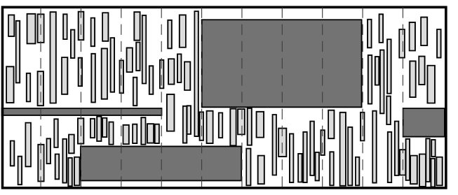
Figure 2.3: An example of a packing after the short-narrow rectangles have been removed, and the wide rectangles (in dark grey) have been aligned to the $M$ vertical strips. Note that the short-high rectangles (in light gray) are much smaller than the vertical strips.

We draw vertical lines across the $1\times(1+2\delta)$ region spaced by $\delta^{2}$, splitting it into $M:=\frac{1+2\delta}{\delta^{2}}$ vertical strips (see Figure 2.3). Consider each maximal rectangular region which is contained in one such strip and does not overlap any wide rectangle; we define a box for each such region that contains at least one short-high rectangle, and we denote the set of such boxes by $\mathcal{B}$.

Note that some short rectangles might intersect the vertical edges of the boxes, but in this case they overlap with exactly two boxes. Using a standard shifting technique, we can assume that no rectangle is cut by the boxes by losing profit at most $\varepsilon_{ra}OPT$: first, we assume that the rectangles intersecting two boxes belong to the leftmost of those boxes. For each box $B\in\mathcal{B}$ (which has width $\delta^{2}$ by definition), we divide it into vertical strips of width $\mu$. Since there are $\frac{\delta^{2}}{\mu}>2/\varepsilon_{ra}$ strips and each rectangle overlaps with at most $2$ such strips, there must exist one of them such that the profit of the rectangles intersecting it is at most $2\mu p(B)\leq\varepsilon_{ra}p(B)$, where $p(B)$ is the profit of all the rectangles that are contained in or belong to $B$. We can remove all the rectangles overlapping such strip, creating in $B$ an empty vertical gap of width $\mu$, and then we can move all the rectangles intersecting the right boundary of $B$ to the empty space, as depicted in Figure 2.4.

Proposition 17.

The number of boxes in $\mathcal{B}$ is at most $\frac{1+2\delta}{\delta^{2}}\cdot\frac{1}{\delta}\leq\frac{2}{\delta^{3}}$.

First, by a shifting argument similar to above, we can reduce the width of each box to $\delta^{2}-\delta^{4}$ while losing only an $\varepsilon_{ra}$ fraction of the profit of the rectangles in $B$. Then, for each $B\in\mathcal{B}$, since the maximum width of the rectangles in $B$ is at most $\mu$, by applying Lemma 15 with $\overline{\varepsilon}=\delta^{2}/2$ we obtain that the rectangles packed inside $B$ can be repacked into a box $B^{\prime}$ of height $h(B)$ and width at most $w^{\prime}(B)\leq\max\{\delta^{2}-\delta^{4}+\frac{72}{\delta^{4}}\mu,(\delta^{2}-\delta^{4})(1+\frac{\delta^{2}}{2})+\frac{76}{\delta^{4}}\mu\}\leq\delta^{2}$, which is true if we make sure that $\mu\leq\delta^{10}/76$. Furthermore, the short-high rectangles in $B$ are packed into at most $\dfrac{216}{\delta^{6}}\leq\dfrac{1}{\delta^{7}}$ vertical containers, assuming without loss of generality that $\delta\leq 1/216$. Note that all the rectangles are packed into vertical containers, because rectangles that have both width and height smaller than $\overline{\varepsilon}$ are short-narrow and we removed them. Summarizing:

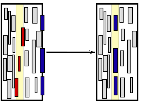
Figure 2.4: For each vertical box, we can remove a low profit subset of rectangles (red in the picture), to make space for short-high rectangles that cross the right edge of the box (blue).

Proposition 18.

There is a set $I^{+}\subseteq I^{\prime}$ of rectangles with total profit at least $(1-O(\varepsilon_{ra}))\cdot p(I^{\prime})$ and a corresponding packing for them in a $1\times(1+2\delta)$ region such that:

• every wide rectangle in $I^{+}$ has its length rounded up to the nearest multiple of $\delta^{2}$ and it is positioned so that its left side is at a position $x$ which is a multiple of $\delta^{2}$, and

• each box $B\in\mathcal{B}$ storing at least one short-high rectangle has width $\delta^{2}$, and the rectangles inside are packed into at most $1/\delta^{7}$ vertical containers.

2.5.2 Fractional packing with $O(1)$ containers

Let us consider now the set of rectangles $I^{+}$ and an almost optimal packing $S^{+}$ for them according to Proposition 18. We remove the rectangles assigned to boxes in $\mathcal{B}$ and consider each box $B\in\mathcal{B}$ as a single pseudoitem. Thus, in the new almost optimal solution there are just pseudoitems from $\mathcal{B}$ and wide rectangles with right and left coordinates that are multiples of $\delta^{2}$. We will now show that we can derive a fractional packing with the same profit, and such that the rectangles and pseudoitems can be (fractionally) assigned to a constant number of containers. By fractional packing we mean a packing where horizontal rectangles are allowed to be sliced horizontally (but not vertically); we can think of the profit as being split proportionally to the heights of the slices.

Let $\mathcal{K}$ be a subset of the horizontal rectangles of size $K$ that will be specified later. By extending horizontally the top and bottom edges of the rectangles in $\mathcal{K}$ and the pseudoitems in $\mathcal{B}$, we partition the knapsack into at most $2(|K|+|\mathcal{B}|)+1\leq 2(K+\frac{2}{\delta^{3}})+1\leq 2(K+\frac{3}{\delta^{3}})$ horizontal stripes.

Let us focus on the (possibly sliced) rectangles contained in one such stripe of height $h$. For any vertical coordinate $y\in[0,h]$ we can define the configuration at coordinate $y$ as the set of positions where the horizontal line at distance $y$ from the bottom cuts a vertical edge of a horizontal rectangle which is not in $\mathcal{K}$. There are at most $2^{M-1}$ possible configurations in a stripe.

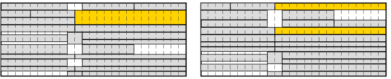
Figure 2.5: Rearranging the rectangles in a horizontal stripe. On the right, rectangles are repacked so that regions with the same configuration appear next to each other. Note that the yellow rectangle has been sliced, since it partakes in two regions with different configurations.

We can further partition the stripe in maximal contiguous regions with the same configuration. Note that the number of such regions is not bounded, since configurations can be repeated. But since the rectangles are allowed to be sliced, we can rearrange the regions so that all the ones with the same configuration appear next to each other; see Figure 2.5 for an example. After this step is completed, we define up to $M$ horizontal containers per each configuration, where we repack the sliced horizontal rectangles. Clearly, all sliced rectangles are repacked.

Thus, the number of horizontal containers that we defined per each stripe is bounded by $M2^{M-1}$, and the total number overall is at most

$$2\left(K+\frac{3}{\delta^{3}}\right)M2^{M-1}=\left(K+\frac{3}{\delta^{3}}\right)M2^{M}.$$

2.5.3 Existence of an integral packing

We will now show the existence of an integral packing, at a small loss of profit.

Consider a fractional packing in $N$ containers. Since each rectangle slice is packed in a container of exactly the same width, it is possible to pack all but at most $N$ rectangles integrally by a simple greedy algorithm: choose a container, and greedily pack in it rectangles of the same width, until either there are no rectangles left for that width, or the next rectangle does not fit in the current container. In this case, we discard this rectangle and close the container, meaning that we do not use it further. Clearly, only one rectangle per container is discarded, and no rectangle is left unpacked.

The only problem is that the total profit of the discarded rectangles can be large. To solve this problem, we use the following shifting argument. Let $\mathcal{K}_{0}=\emptyset$ and $K_{0}=0$. For convenience, let us define $f(K)=\left(K+\frac{3}{\delta^{3}}\right)M2^{M}$.

First, consider the fractional packing obtained by choosing $\mathcal{K}=\mathcal{K}_{0}$, so that $K=K_{0}=0$. Let $\mathcal{K}_{1}$ be the set of discarded rectangles obtained by the greedy algorithm, and let $K_{1}=|\mathcal{K}_{1}|$. Clearly, by the above reasoning, the number of discarded rectangles is bounded by $f(K_{0})$. If the profit $p(\mathcal{K}_{1})$ of the discarded rectangles is at most $\varepsilon_{ra}p(OPT)$, then we remove them and there is nothing else to prove. Otherwise, consider the fractional packing obtained by fixing $\mathcal{K}=\mathcal{K}_{0}\cup\mathcal{K}_{1}$. Again, we will obtain a set $\mathcal{K}_{2}$ of discarded rectangles such that $K_{2}:=|\mathcal{K}_{2}|\leq f(K_{0}+K_{1})$. Since the sets $\mathcal{K}_{1},\mathcal{K}_{2},\dots$ that we obtain are all disjoint, the process must stop after at most $1/\varepsilon_{ra}$ iterations. Setting $p:=M2^{M}$ and $q:=\frac{3}{\delta^{3}}M2^{M}$, we have that $K_{i+1}\leq p(K_{0}+K_{1}+\dots K_{i})+q$ for each $i\geq 0$. Crudely bounding it as $K_{i+1}\leq i\cdot pq\cdot K_{i}$, we immediately obtain that $K_{i}\leq(pq)^{i}$. Thus, in the successful iteration, the size of $\mathcal{K}$ is at most $K_{1/\varepsilon_{ra}-1}$ and the number of containers is at most $K_{1/\varepsilon_{ra}}\leq(pq)^{1/\varepsilon_{ra}}=(\frac{3}{\delta^{2}}M^{2}2^{2M})^{1/\varepsilon_{ra}}=O_{\varepsilon_{ra},\delta}(1)$.

2.5.4 Rounding down horizontal and vertical containers

As per the above analysis, the total number of horizontal containers is at most $(\frac{3}{\delta^{2}}M^{2}2^{2M})^{\varepsilon_{ra}}$ and the total number of vertical containers is at most $\frac{2}{\delta^{3}}\cdot\frac{1}{\delta^{7}}=\frac{2}{\delta^{10}}$.

We will now show that, at a small loss of profit, it is possible to replace each horizontal and each vertical container defined so far with a constant number of smaller containers, so that the total area of the new containers is at most as big as the total area of the rectangles originally packed in the container. Note that in each container we consider the rectangles with the original widths (not rounded up). We use the following lemma:

Lemma 19.

Let $C$ be a horizontal (resp. vertical) container defined above, and let $\mathcal{R}_{C}$ be the set of rectangles packed in $C$. Then, it is possible to pack a set $\mathcal{R}^{\prime}_{C}\subseteq\mathcal{R}_{C}$ of profit at least $(1-3\varepsilon_{ra})p(\mathcal{R}_{C})$ in a set of at most $\left\lceil\log_{1+\varepsilon_{ra}}(\frac{1}{\delta})\right\rceil/\varepsilon_{ra}^{2}$ horizontal (resp. vertical) containers that can be packed inside $C$ and such that their total area is at most $a(\mathcal{R}_{C})$.

Proof.

Without loss of generality, we prove the result only for the case of a horizontal container.

Since $w_{i}\geq\delta$ for each rectangle $R_{i}\in\mathcal{R}_{C}$, we can partition the rectangles in $\mathcal{R}_{C}$ into at most $\left\lceil\log_{1+\varepsilon_{ra}}(\frac{1}{\delta})\right\rceil$ groups $\mathcal{R}_{1},\mathcal{R}_{2},\dots$, so that in each $\mathcal{R}_{j}$ the widest rectangle has width bigger than the smallest by a factor at most $1+\varepsilon_{ra}$; we can then define a container $C_{j}$ for each group $\mathcal{R}_{j}$ that has the width of the widest rectangle it contains and height equal to the sum of the heights of the contained rectangles.

Consider now one such $C_{j}$ and the set of rectangles $\mathcal{R}_{j}$ that it contains, and let $P:=p(\mathcal{R}_{j})$. Clearly, $w(C_{j})\leq(1+\varepsilon_{ra})w_{i}$ for each $R_{i}\in\mathcal{R}_{j}$, and so $a(C_{j})\leq(1+\varepsilon_{ra})a(\mathcal{R}_{j})$. If all the rectangles in $\mathcal{R}_{j}$ have height at most $\varepsilon_{ra}h(C_{j})$, then we can remove a set of rectangles with total height at least $\varepsilon_{ra}h(C)$ and profit at most $2\varepsilon_{ra}p(\mathcal{R}_{j})$. Otherwise, let $\mathcal{Q}$ be the set of rectangles of height larger than $\varepsilon_{ra}h(C_{j})$, and note that $a(Q)\geq\varepsilon_{ra}h(C_{j})w(C_{j})/(1+\varepsilon_{ra})$. If $p(\mathcal{Q})\leq\varepsilon_{ra}P$, then we remove the rectangles in $\mathcal{Q}$ from the container $C_{j}$ and reduce its height as much as possible, obtaining a smaller container $C^{\prime}_{j}$; since $a(C^{\prime}_{j})\leq a(C_{j})-\varepsilon_{ra}a(C_{j})=(1-\varepsilon_{ra})a(C_{j})\leq(1-\varepsilon_{ra})(1+\varepsilon_{ra})a(\mathcal{R}_{j})<a(\mathcal{R}_{j})$, then the proof is finished. Otherwise, we define one container for each of the rectangles in $\mathcal{Q}$ (which are at most $1/\varepsilon_{ra}$) of exactly the same size, and we still shrink the container with the remaining rectangles as before; note that there is no lost area for each of the newly defined container. Since at every non-terminating iteration a set of rectangles with profit larger than $\varepsilon_{ra}P$ is removed, the process must end within $1/\varepsilon_{ra}$ iterations.

Note that the total number of containers that we produce for each initial container $C_{j}$ is at most $1/\varepsilon_{ra}^{2}$, and this concludes the proof. ∎

Thus, by applying the above lemma to each horizontal and each vertical container, we obtain a modified packing where the total area of the horizontal and vertical containers is at most the area of the rectangles of $\mathcal{R}^{\prime}$ (without the short-narrow rectangles, which we will take into account in the next section), while the number of containers increases at most by a factor $\left\lceil\log_{1+\varepsilon_{ra}}(\frac{1}{\delta})\right\rceil/\varepsilon_{ra}^{2}$.

2.5.5 Packing short-narrow rectangles

Consider the integral packing obtained from the previous section, which has at most $K^{\prime}:=\left(\frac{2}{\delta^{10}}+(\frac{3}{\delta^{2}}M^{2}2^{2M})^{\varepsilon_{ra}}\right)\left\lceil\log_{1+\varepsilon_{ra}}(\frac{1}{\delta})\right\rceil/\varepsilon_{ra}^{2}$ containers. We can create a non-uniform grid extending each side of the containers until they hit another container or the boundary of the knapsack. Moreover, we also add horizontal and vertical lines spaced at distance $\varepsilon_{ra}$. We call free cell each face defined by the above lines that does not overlap a container of the packing; by construction, no free cell has a side bigger than $\varepsilon_{ra}$. The number of free cells in this grid plus the existing containers is bounded by $K_{TOTAL}={(2K^{\prime}+1/\varepsilon_{ra})}^{2}=O_{\varepsilon_{ra},\delta}(1)$. We crucially use the fact that this number does not depend on the value of $\mu$.

Note that the total area of the free cells is no less than the total area of the short-narrow rectangles, as a consequence of the guarantees on the area of the containers introduced so far. We will pack the short-narrow rectangles into the free cells of this grid using NFDH, but we only use cells that have width and height at least $\frac{8\mu}{\varepsilon_{ra}}$; thus, each short-narrow rectangle will be assigned to a cell whose width (resp. height) is larger by at least a factor $8/\varepsilon_{ra}$ than the width (resp. height) of the rectangle. Each discarded cell has area at most $\frac{8\mu}{\varepsilon_{ra}}$, which implies that the total area of discarded cells is at most $\frac{8\mu K_{TOTAL}}{\varepsilon_{ra}}$. Now we consider the selected cells in an arbitrary order and pack short narrow rectangles into them using NFDH, defining a new area container for each cell that is used. Thanks to Lemma 1, we know that each new container $C$ (except maybe the last one) that is used by NFDH contains rectangles for a total area of at least $(1-\varepsilon_{ra}/4)a(C)$. Thus, if all rectangles are packed, we remove the last container opened by NFDH, and we call $S$ the set of rectangles inside, that we will repack elsewhere; note that $a(S)\leq\varepsilon_{ra}^{2}\leq\varepsilon_{ra}/3$, since all the rectangles in $S$ were packed in a free cell. Instead, if not all rectangles are packed by NFDH, let $S$ be the residual rectangles. In this case, the area of the unpacked rectangles is $a(S)\leq\frac{8\mu K_{TOTAL}}{\varepsilon_{ra}}+\varepsilon_{ra}/4\leq\varepsilon_{ra}/3$, assuming that $\mu\leq\frac{\varepsilon_{ra}^{2}}{96K_{TOTAL}}$.

In order to repack the rectangles of $S$, we define a new area container $C_{S}$ of height $1$ and width $\varepsilon_{ra}/2$. Since $a(C_{S})=\varepsilon_{ra}/2\geq(\varepsilon_{ra}/3)/(1-2\varepsilon_{ra})$, all elements from $S$ are packed in $C_{S}$ by NFDH, and the container can be added to the knapsack by further enlarging its width from $1+2\delta$ to $1+2\delta+\varepsilon_{ra}/2<1+\varepsilon_{ra}$.

The last required step is to guarantee the necessary constraint on the total area of the area containers, similarly to what was done in Section 2.5.4 for the horizontal and vertical containers.

Let $D$ be any full area container (that is, any area container except for $C_{S}$). We know that the area of the rectangles $R_{D}$ in $D$ is $a(R_{D})\geq(1-\varepsilon_{ra})a(D)$, since each rectangle $R_{i}$ inside $D$ has width less than $\varepsilon_{ra}w(D)/2$ and height less than $\varepsilon_{ra}h(D)/2$, by construction. We remove rectangles from $R_{D}$ in non-decreasing order of profit/area ratio, until the total area of the residual rectangles is between $(1-4\varepsilon_{ra})a(D)$ and $(1-3\varepsilon_{ra})a(D)$ (this is possible, since each element has area at most $\varepsilon_{ra}^{2}a(D)$); let $R^{\prime}_{D}$ be the resulting set. We have that $p(R^{\prime}_{D})\geq(1-4\varepsilon_{ra})p(R_{D})$, due to the greedy choice. Let us define a container $D^{\prime}$ of width $w(D)$ and height $(1-\varepsilon_{ra})h(D)$. It is easy to verify that each rectangle in $R_{D}$ has width (resp. height) at most $\varepsilon_{ra}w(D^{\prime})$ (resp. $\varepsilon_{ra}h(D^{\prime})$). Moreover, since $a(R^{\prime}_{D})\leq(1-3\varepsilon_{ra})a(D)\leq(1-2\varepsilon_{ra})(1-\varepsilon_{ra})a(C)\leq(1-2\varepsilon_{ra})a(C^{\prime})$, then all elements in $R^{\prime}_{D}$ are packed in $D^{\prime}$. By applying this reasoning to each area container (except $C_{S}$), we obtain property (3) of Lemma 14.

Note that the constraints on $\mu$ and $\delta$ that we imposed are $\mu\leq\frac{\delta^{10}}{76}$ (from Section 2.5.1), and $\mu\leq\frac{\varepsilon_{ra}^{2}}{96K_{TOTAL}}$. It is easy to check that both of them are satisfied if we choose $f(x)=(\varepsilon_{ra}x)^{C}$ for a big enough constant $C$ that depends only on $\varepsilon_{ra}$. This concludes the proof.

Chapter 3 A PPT $(4/3+\varepsilon)$-approximation for Strip Packing

In this chapter, we present a $(\frac{4}{3}+\varepsilon)$-approximation for Strip Packing running in pseudo-polynomial time. These results are published in Gálvez, Grandoni, Ingala and Khan [2016].

Our approach refines the technique of Nadiradze and Wiese [2016]. Like many results in the field, it is based on finding some particular type of packings that have a special structure, and that can consequently be approximated more efficiently.

Let $\alpha\in[1/3,1/2)$ be a proper constant parameter, and define a rectangle $R_{i}$ to be tall if $h_{i}>\alpha\cdot OPT$, where $OPT$ is the height of an optimal packing. They prove that the optimal packing can be structured into a constant number of axis-aligned rectangular regions (boxes), that occupy a total height of $OPT^{\prime}\leq(1+\varepsilon)OPT$ inside the vertical strip. Some rectangles are not fully contained into one box (they are cut by some box). Among them, tall rectangles remain in their original position. All the other cut rectangles are repacked on top of the boxes: part of them in a horizontal box of size $W\times O(\varepsilon)OPT$, and the remaining ones in a vertical box of size $O(\varepsilon W)\times\alpha\,OPT$ (that we next imagine as placed on the top-left of the packing under construction).

Some of these boxes contain only relatively high rectangles (including tall ones) of relatively small width. The next step is a rearrangement of the rectangles inside one such vertical box $\overline{B}$ (see Figure 3.4(a)), say of size $\overline{w}\times\overline{h}$: they first slice non-tall rectangles into unit width rectangles (this slicing can be finally avoided with standard techniques). Then they shift tall rectangles to the top/bottom of $\overline{B}$, shifting sliced rectangles consequently (see Figure 3.4(b)). Now they discard all the (sliced) rectangles completely contained in a central horizontal region of size $\overline{w}\times(1+\varepsilon-2\alpha)\overline{h}$, and they nicely rearrange the remaining rectangles into a constant number of sub-boxes (excluding possibly a few more non-tall rectangles, that can be placed in the additional vertical box).

These discarded rectangles can be packed into $2$ extra boxes of size $\frac{\overline{w}}{2}\times(1+\varepsilon-2\alpha)\overline{h}$ (see Figure 3.4(d)). In turn, the latter boxes can be packed into two discarded boxes of size $\frac{W}{2}\times(1+\varepsilon-2\alpha)OPT^{\prime}$, that we can imagine as placed, one on top of the other, on the top-right of the packing. See Figure 3.1(a) for an illustration of the final packing. This leads to a total height of $(1+\max\{\alpha,2(1-2\alpha)\}+O(\varepsilon))\cdot OPT$, which is minimized by choosing $\alpha=\frac{2}{5}$.

(a) Final packing obtained by
Nadiradze and Wiese [2016].

(b) Final packing obtained in this work.
Here $\gamma$ is a small constant depending on $\varepsilon$.

Figure 3.1: Comparison of final solutions.

Our main technical contribution is a repacking lemma that allows one to repack a small fraction of the discarded rectangles of a given box inside the free space left by the corresponding sub-boxes (while still having $O_{\varepsilon}(1)$ many sub-boxes in total). This is illustrated in Figure 3.4(e). This way we can pack all the discarded rectangles into a single discarded box of size $(1-\gamma)W\times(1+\varepsilon-2\alpha)OPT^{\prime}$, where $\gamma$ is a small constant depending on $\varepsilon$, that we can place on the top-right of the packing. The vertical box where the remaining rectangles are packed still fits to the top-left of the packing, next to the discarded box. See Figure 3.1(b) for an illustration. Choosing $\alpha=1/3$ gives the claimed approximation factor.

We remark that the basic approach by Nadiradze and Wiese strictly requires that at most $2$ tall rectangles can be packed one on top of the other in the optimal packing, hence imposing $\alpha\geq 1/3$. Thus in some sense we pushed their approach to its limit.

The algorithm by Nadiradze and Wiese [2016] is not directly applicable to the case when $90^{\circ}$ rotations are allowed. In particular, they use a linear program to pack some rectangles. When rotations are allowed, it is unclear how to decide which rectangles are packed by the linear program. We use a combinatorial container-based approach to circumvent this limitation, which allows us to pack all the rectangles using dynamic programming. In this way we obtain a PPT $(4/3+\varepsilon)$-approximation for strip packing with rotations, breaking the polynomial-time approximation barrier of 3/2 for that variant as well.

3.1 Preliminaries and notations

We will follow the notation from Nadiradze and Wiese [2016], which will be explained as it is needed.

Recall that $OPT\in\mathbb{N}$ denotes the height of the optimal packing for instance $\mathcal{R}$. By trying all the pseudo-polynomially many possibilities, we can assume that $OPT$ is known to the algorithm. Given a set $\mathcal{M}\subseteq\mathcal{R}$ of rectangles, $a(\mathcal{M})$ will denote the total area of rectangles in $\mathcal{M}$, i.e., $a(\mathcal{M})=\sum_{R_{i}\in\mathcal{M}}{h_{i}\cdot w_{i}}$, and $h_{\max}(\mathcal{M})$ (resp. $w_{\max}(\mathcal{M})$) denotes the maximum height (resp. width) of rectangles in $\mathcal{M}$. Throughout this work, a box of size $a\times b$ means an axis-aligned rectangular region of width $a$ and height $b$.

3.1.1 Classification of rectangles

Let $0<\varepsilon<\alpha$, and assume for simplicity that $\frac{1}{\varepsilon}\in\mathbb{N}$. We first classify the input rectangles into six groups according to parameters $\delta_{h},\delta_{w},\mu_{h},\mu_{w}$ satisfying $\varepsilon\geq\delta_{h}>\mu_{h}>0$ and $\varepsilon\geq\delta_{w}>\mu_{w}>0$, whose values will be chosen later (see also Figure 3.2). A rectangle $R_{i}$ is:

Figure 3.2: Classification of the rectangles. Each rectangle is represented as a point whose $x$ (resp., $y$) coordinate indicates its width (resp., height).

• Large if $h_{i}\geq\delta_{h}OPT$ and $w_{i}\geq\delta_{w}W$.

• Tall if $h_{i}>\alpha OPT$ and $w_{i}<\delta_{w}W$.

• Vertical if $h_{i}\in[\delta_{h}OPT,\alpha OPT]$ and $w_{i}\leq\mu_{w}W$,

• Horizontal if $h_{i}\leq\mu_{h}OPT$ and $w_{i}\geq\delta_{w}W$,

• Small if $h_{i}\leq\mu_{h}OPT$ and $w_{i}\leq\mu_{w}W$;

• Medium in all the remaining cases, i.e., if $h_{i}\in(\mu_{h}OPT,\delta_{h}OPT)$, or $w_{i}\in(\mu_{w}W,\delta_{w}W)$ and $h_{i}\leq\alpha OPT$.

We use $L$, $T$, $V$, $H$, $S$, and $M$ to denote the sets of large, tall, vertical, horizontal, small, and medium rectangles, respectively. We remark that, differently from Nadiradze and Wiese [2016], we need to allow $\delta_{h}\neq\delta_{w}$ and $\mu_{h}\neq\mu_{w}$ due to some additional constraints in our construction.

Notice that according to this classification, every vertical line across the optimal packing intersects at most two tall rectangles. The following lemma allows us to choose $\delta_{h},\delta_{w},\mu_{h}$ and $\mu_{w}$ in such a way that $\delta_{h}$ and $\mu_{h}$ ($\delta_{w}$ and $\mu_{w}$, respectively) differ by a large factor, and medium rectangles have small total area.

Lemma 20.

Given a polynomial-time computable function $f:(0,1)\rightarrow(0,1)$, with $f(x)<x$, any constant $\varepsilon\in(0,1)$, and any positive integer $k$, we can compute in polynomial time a set $\Delta$ of $T=2(\frac{1}{\varepsilon})^{k}$ many positive real numbers upper bounded by $\varepsilon$, such that there is at least one number $\delta_{h}\in\Delta$ so that $a(M)\leq\varepsilon^{k}\cdot OPT\cdot W$ by choosing $\mu_{h}=f(\delta_{h})$, $\mu_{w}=\frac{\varepsilon\mu_{h}}{12}$, and $\delta_{w}=\frac{\varepsilon\delta_{h}}{12}$.

Proof.

Let $T=2(\frac{1}{\varepsilon})^{k}$. Let $y_{1}=\varepsilon$, and, for each $j\in[T]$, define $y_{j+1}=f(y_{j})$. Let $x_{j}=\frac{\varepsilon y_{j}}{12}$. For each $j\leq T$, let $W_{j}=\{R_{i}\in\mathcal{R}:w_{i}\in[x_{i+1},x_{i})\}$ and similarly $H_{j}=\{R_{i}\in\mathcal{R}:h_{i}\in[y_{i+1},y_{i})\}$. Observe that $W_{j^{\prime}}$ is disjoint from $W_{j^{\prime\prime}}$ (resp. $H_{j^{\prime}}$ is disjoint from $H_{j^{\prime\prime}}$) for every $j^{\prime}\neq j^{\prime\prime}$, and the total area of rectangles in $\bigcup W_{i}$ ($\bigcup H_{i}$ respectively) is at most $W\cdot OPT$. Thus, there exists a value $\overline{j}$ such that the total area of the elements in $W_{\overline{j}}\cup H_{\overline{j}}$ is at most $\dfrac{2OPT\cdot W}{T}=\varepsilon^{k}\cdot OPT\cdot W$. Choosing $\delta_{h}=y_{\overline{j}}$, $\mu_{h}=y_{\overline{j}+1}$, $\delta_{w}=x_{\overline{j}}$, $\mu_{w}=x_{\overline{j}+1}$ verifies all the conditions of the lemma. ∎

The function $f$ and the constant $k$ will be chosen later. From now on, assume that $\delta_{h},\delta_{w},\mu_{h}$ and $\mu_{w}$ are chosen according to Lemma 20.

3.1.2 Overview of the construction

We next overview some of the basic results in Nadiradze and Wiese [2016] that are needed in our result. We define the constant $\gamma:=\frac{\varepsilon\delta_{h}}{2}$, and we assume without loss of generality that $\gamma\cdot OPT\in\mathbb{N}$.

Let us forget for a moment about the small rectangles in $S$. We will pack all the remaining rectangles $L\cup H\cup T\cup V\cup M$ into a sufficiently small number of boxes embedded into the strip. By standard techniques, as in Nadiradze and Wiese [2016], it is then possible to pack $S$ (essentially using NFDH in a proper grid defined by the above boxes) while increasing the total height at most by $O(\varepsilon)OPT$. See Section 3.4 for more details on packing of small rectangles.

The following lemma from Nadiradze and Wiese [2016] allows one to round the heights and positions of rectangles of large enough height, without increasing much the height of the packing.

Lemma 21 (Nadiradze and Wiese [2016]).

There exists a feasible packing of height $OPT^{\prime}\leq(1+\varepsilon)OPT$ where: (1) the height of each rectangles in $L\cup T\cup V$ is rounded up to the closest integer multiple of $\gamma\cdot OPT$ and (2) their $x$-coordinates are as in the optimal solution and their $y$-coordinates are integer multiples of $\gamma\cdot OPT$.

We next focus on rounded rectangle heights (that is, we implicitly replace $L\cup T\cup V$ with their rounded version) and on this slightly suboptimal solution of height $OPT^{\prime}$.

The following lemma helps us to pack rectangles in $M$.

Lemma 22.

If $k$ in Lemma 20 is chosen sufficiently large, all the rectangles in $M$ can be packed in polynomial time into a box $B_{M,hor}$ of size $W\times O(\varepsilon)OPT$ and a box $B_{M,ver}$ of size $(\frac{\gamma}{3}W)\times(\alpha OPT)$. Furthermore, there is one such packing using $\frac{3\varepsilon}{\mu_{h}}$ vertical containers in $B_{M,hor}$ and $\frac{\gamma}{3\mu_{w}}$ horizontal containers in $B_{M,ver}$.

Proof.

We first pack rectangles in $\mathcal{A}:=\{R_{i}\in M:h_{i}\in(\mu_{h}OPT,\delta_{h}OPT)\}$ using NFDH. From Lemma 2 we know that the height of the packing is at most $h_{\max}(\mathcal{A})+\frac{2\cdot a(\mathcal{A})}{W}$. Since $h_{max}(\mathcal{A})\leq\delta_{h}OPT<\varepsilon OPT$ and $a(\mathcal{A})\leq a(M)\leq\varepsilon^{k}\cdot OPT\cdot W\leq\varepsilon\cdot OPT\cdot W$, because of Lemma 20, the resulting packing fits into a box $B_{M,hor}$ of size $W\times(3\varepsilon\cdot OPT)$. As $h_{i}\geq\mu_{h}OPT$, the number of shelves used by NFDH is at most $\frac{3\varepsilon}{\mu_{h}}$: this also bounds the number of vertical containers needed.

We next pack $\mathcal{A}^{\prime}:=M\setminus\mathcal{A}$ into a box $B_{M,ver}$ of size $(\frac{\gamma}{3}W)\times(\alpha OPT)$. Recall that $\gamma:=\frac{\varepsilon\delta_{h}}{2}$. Note that, for each $R_{i}\in\mathcal{A}^{\prime}$, we have $w_{i}\in(\mu_{w}W,\delta_{w}W)$ and $h_{i}\leq\alpha OPT$. By ideally rotating the box and the rectangles by $90^{\circ}$, we can apply the NFDH algorithm. Lemma 2 implies that we can pack all the rectangles if the width of the box is at least $w_{\max}(\mathcal{A}^{\prime})+\frac{2a(\mathcal{A}^{\prime})}{\alpha OPT}$. Now observe that

$$w_{\max}(\mathcal{A}^{\prime})\leq\delta_{w}W=\frac{\varepsilon\delta_{h}}{12}W=\frac{\gamma}{6}W$$

and also, since $\alpha\geq 1/3$:

$$\frac{2a(\mathcal{A}^{\prime})}{\alpha OPT}\leq\frac{6a(\mathcal{A}^{\prime})}{OPT}\leq 6\varepsilon^{k}W\leq\frac{\gamma}{6}W,$$

where the last inequality is true for any $k\geq\log_{1/\varepsilon}{(36/\gamma)}$. Similarly to the previous case, the number of shelves is at most $\frac{\gamma}{3\mu_{w}}$. Thus all the rectangles can be packed into at most $\frac{\gamma}{3\mu_{w}}$ horizontal containers. ∎

We say that a rectangle $R_{i}$ is cut by a box $B$ if both $R_{i}\setminus B$ and $B\setminus R_{i}$ are non-empty (considering both $R_{i}$ and $B$ as open regions with an implicit embedding on the plane). We say that a rectangle $R_{i}\in H$ (resp. $R_{i}\in T\cup V$) is nicely cut by a box $B$ if $R_{i}$ is cut by $B$ and their intersection is a rectangular region of width $w_{i}$ (resp. height $h_{i}$). Intuitively, this means that an edge of $B$ cuts $R_{i}$ along its longest side (see Figure 3.3).

Figure 3.3: A box and some overlapping rectangles. Dark gray rectangles are nicely cut by the box; hatched rectangles are cut but not nicely cut by the box, and light gray rectangle is not cut by the box.

Now it remains to pack $L\cup H\cup T\cup V$: The following lemma, taken from Nadiradze and Wiese [2016] modulo minor technical adaptations, describes an almost optimal packing of those rectangles.

Lemma 23.

There is an integer $K_{B}=(\frac{1}{\varepsilon})(\frac{1}{\delta_{w}})^{O(1)}$ such that, assuming $\mu_{h}\leq\frac{\varepsilon\delta_{w}}{K_{B}}$, there is a partition of the region $B_{OPT^{\prime}}:=[0,W]\times[0,OPT^{\prime}]$ into a set $\mathcal{B}$ of at most $K_{B}$ boxes and a packing of the rectangles in $L\cup T\cup V\cup H$ such that:

• each box has size equal to the size of some $R_{i}\in L$ (large box), or has height at most $\delta_{h}OPT^{\prime}$ (horizontal box), or has width at most $\delta_{w}W$ (vertical box);

• each $R_{i}\in L$ is contained into a large box of the same size;

• each $R_{i}\in H$ is contained into a horizontal box or is cut by some box. Furthermore, the total area of horizontal cut rectangles is at most $W\cdot O(\varepsilon)OPT^{\prime}$;

• each $R_{i}\in T\cup V$ is contained into a vertical box or is nicely cut by some vertical box.

Proof.

We apply Lemma 6 in Nadiradze and Wiese [2016], where we set the parameter $\delta$ to $\delta_{w}$. Recall that $\delta_{w}<\delta_{h}$; by requiring that $\mu_{h}<\delta_{w}$, and since rectangles with height in $[\delta_{w},\delta_{h})$ are in $M$, we have that $\{R_{i}\in\mathcal{R}\setminus M\,:\,w_{i}\geq\delta_{h}W\mbox{ and }h_{i}\geq\delta_{h}OPT\}=\{R_{i}\in\mathcal{R}\setminus M\,:\,w_{i}\geq\delta_{w}W\mbox{ and }h_{i}\geq\delta_{h}OPT\}$.

Let $H_{cut}\subseteq H$ be the set of horizontal rectangles that are nicely cut by a box. Since rectangles in $H_{cut}$ satisfy $w_{i}\geq\delta_{w}W$, at most $\frac{2}{\delta_{w}}$ of them are nicely cut by a box, and there are at most $K_{B}$ boxes. Hence, their total area is at most $\frac{\mu_{h}OPT\cdot W\cdot 2K_{B}}{\delta_{w}}$, which is at most $2\varepsilon\cdot OPT\cdot W$, provided that $\mu_{h}\leq\varepsilon\cdot\frac{\delta_{w}}{K_{B}}$. Since Lemma 6 in Nadiradze and Wiese [2016] implies that the area of the cut horizontal rectangles that are not nicely cut is at most $\varepsilon OPT^{\prime}\cdot W$, the total area of horizontal cut rectangles is at most $3\varepsilon OPT^{\prime}\cdot W$. ∎

We denote the sets of vertical, horizontal, and large boxes by $\mathcal{B}_{V},\mathcal{B}_{H}$ and $\mathcal{B}_{L}$, respectively. Observe that $\mathcal{B}$ can be guessed in PPT. We next use $T_{cut}\subseteq T$ and $V_{cut}\subseteq V$ to denote tall and vertical cut rectangles in the above lemma, respectively. Let us also define $T_{box}=T\setminus T_{cut}$ and $V_{box}=V\setminus V_{cut}$.

Using standard techniques (see e.g. Nadiradze and Wiese [2016]), we can pack all the rectangles excluding the ones contained in vertical boxes in a convenient manner. This is summarized in the following lemma.

Lemma 24.

Given $\mathcal{B}$ as in Lemma 23 and assuming $\mu_{w}\leq\frac{\gamma\delta_{h}}{6K_{B}(1+\varepsilon)}$, there exists a packing of $L\cup H\cup T\cup V$ such that:

1. all the rectangles in $L$ are packed in $\mathcal{B}_{L}$;

2. all the rectangles in $H$ are packed in $\mathcal{B}_{H}$ plus an additional box $B_{H,cut}$ of size $W\times O(\varepsilon)OPT$;

3. all the rectangles in $T_{cut}\cup T_{box}\cup V_{box}$ are packed as in Lemma 23;

4. all the rectangles in $V_{cut}$ are packed in an additional vertical box $B_{V,cut}$ of size $(\frac{\gamma}{3}W)\times(\alpha OPT)$.

Proof.

Note that there are at most $1/(\delta_{w}\delta_{h})$ rectangles in $L$ and at most $4K_{B}$ rectangles in $T_{cut}$, since the left (resp. right) side of each box can nicely cut at most $2$ tall rectangles; this is enough to prove points (1) and (3).

Thanks to Lemma 23, the total area of horizontal cut rectangles is at most $O(\varepsilon OPT^{\prime}\cdot W)$. By Lemma 1, we can remove them from the packing and pack them in the additional box $B_{H,cut}$ using NFDH algorithm, proving point (2).

Each box of the partition can nicely cut at most $\frac{2(1+\varepsilon)}{\delta_{h}}$ rectangles in $V$; thus, the cut vertical rectangles are at most $\frac{2K_{B}(1+\varepsilon)}{\delta_{h}}$. Since the width of each vertical rectangle is at most $\mu_{w}W$, they can be removed from the packing and placed in $B_{V,cut}$, piled side by side, as long as $\frac{2K_{B}(1+\varepsilon)}{\delta_{h}}\cdot\mu_{w}W\leq\frac{\gamma}{3}W$, which is equivalent to $\mu_{w}\leq\frac{\gamma\delta_{h}}{6K_{B}(1+\varepsilon)}$. This proves point (4). ∎

We will pack all the rectangles (essentially) as in Nadiradze and Wiese [2016], with the exception of $T_{box}\cup V_{box}$ where we exploit a refined approach. This is the technical heart of our result, and it is discussed in the next section.

3.2 A repacking lemma

We next describe how to pack rectangles in $T_{box}\cup V_{box}$. In order to highlight our contribution, we first describe how the approach by Nadiradze and Wiese [2016] works.

It is convenient to assume that all the rectangles in $V_{box}$ are sliced vertically into sub-rectangles of width $1$ each. Let $V_{sliced}$ be such sliced rectangles. We will show how to pack all the rectangles in $T_{box}\cup V_{sliced}$ into a constant number of sub-boxes. Using standard techniques it is then possible to pack $V_{box}$ into the space occupied by $V_{sliced}$ plus an additional box $B_{V,round}$ of size $(\frac{\gamma}{3}W)\times\alpha OPT$. See Lemma 28 for more details.

We next focus on a specific vertical box $\overline{B}$, say of size $\overline{w}\times\overline{h}$ (see Figure 3.4(a)). Let $\overline{T}_{cut}$ be the tall rectangles cut by $\overline{B}$. Observe that there are at most $4$ such rectangles ($2$ on the left/right side of $\overline{B}$). The rectangles in $\overline{T}_{cut}$ are packed as in Lemma 24. Let also $\overline{T}$ and $\overline{V}$ be the tall rectangles and sliced vertical rectangles, respectively, originally packed completely inside $\overline{B}$.

They show that it is possible to pack $\overline{T}\cup\overline{V}$ into a constant size set $\overline{\mathcal{S}}$ of sub-boxes contained inside $\overline{B}-\overline{T}_{cut}$, plus an additional box $\overline{D}$ of size $\overline{w}\times(1+\varepsilon-2\alpha)\overline{h}$. Here $\overline{B}-\overline{T}_{cut}$ denotes the region inside $\overline{B}$ not contained in $\overline{T}_{cut}$. In more detail, they start by considering each rectangle $R_{i}\in\overline{T}$. Since $\alpha\geq\frac{1}{3}$ by assumption, one of the regions above or below $R_{i}$ cannot contain another tall rectangle in $\overline{T}$, say the first case applies (the other one being symmetric). Then we move $R_{i}$ up so that its top side overlaps with the top side of $\overline{B}$. The sliced rectangles in $\overline{V}$ that are covered this way are shifted right below $R$ (note that there is enough free space by construction). At the end of the process all the rectangles in $\overline{T}$ touch at least one of the top and bottom side of $\overline{B}$ (see Figure 3.4(b)). Note that no rectangle is discarded up to this point.

Next, we partition the space inside $\overline{B}-(\overline{T}\cup\overline{T}_{cut})$ into maximal height unit-width vertical stripes. We call each such stripe a free rectangle if both its top and bottom side overlap with the top or bottom side of some rectangle in $\overline{T}\cup\overline{T}_{cut}$, and otherwise a pseudo rectangle (see Figure 3.4(c)). We define the $i$-th free rectangle to be the free rectangle contained in stripe $[i-1,i]\times[0,\overline{h}]$.

Note that all the free rectangles are contained in a horizontal region of width $\overline{w}$ and height at most $\overline{h}-2\alpha OPT\leq\overline{h}-2\alpha\frac{OPT^{\prime}}{1+\varepsilon}\leq\overline{h}(1-\frac{2\alpha}{1+\varepsilon})\leq\overline{h}(1+\varepsilon-2\alpha)$ contained in the central part of $\overline{B}$. Let $\overline{V}_{disc}$ be the set of (sliced vertical) rectangles contained in the free rectangles. Rectangles in $\overline{V}_{disc}$ can be obviously packed inside $\overline{D}$. For each corner $Q$ of the box $\overline{B}$, we consider the maximal rectangular region that has $Q$ as a corner and only contains pseudo rectangles whose top/bottom side overlaps with the bottom/top side of a rectangle in $\overline{T}_{cut}$; there are at most $4$ such non-empty regions, and for each of them we define a corner sub-box, and we call the set of such sub-boxes $\overline{B}_{corn}$ (see Figure 3.4(c)). The final step of the algorithm is to rearrange horizontally the pseudo/tall rectangles so that pseudo/tall rectangles of the same height are grouped together as much as possible (modulo some technical details). The rectangles in $\overline{B}_{corn}$ are not moved. The sub-boxes are induced by maximal consecutive subsets of pseudo/tall rectangles of the same height touching the top (resp., bottom) side of $\overline{B}$ (see Figure 3.4(d)). We crucially remark that, by construction, the height of each sub-box (and of $\overline{B}$) is a multiple of $\gamma OPT$.

By splitting each discarded box $\overline{D}$ into two halves $\overline{B}_{disc,top}$ and $\overline{B}_{disc,bot}$, and replicating the packing of boxes inside $B_{OPT^{\prime}}$, it is possible to pack all the discarded boxes into two boxes $B_{disc,top}$ and $B_{disc,bot}$, both of size $\frac{W}{2}\times(1+\varepsilon-2\alpha)OPT^{\prime}$.

A feasible packing of boxes (and hence of the associated rectangles) of height $(1+\max\{\alpha,2(1-2\alpha)\}+O(\varepsilon))OPT$ is then obtained as follows. We first pack $B_{OPT^{\prime}}$ at the base of the strip, and then on top of it we pack $B_{M,hor}$, two additional boxes $B_{H,round}$ and $B_{H,cut}$ (which will be used to repack the horizontal items), and a box $B_{S}$ (which will be used to pack some of the small items). The latter $4$ boxes all have width $W$ and height $O(\varepsilon OPT^{\prime})$. On the top right of this packing we place $B_{disc,top}$ and $B_{disc,bot}$, one on top of the other. Finally, we pack $B_{M,ver}$, $B_{V,cut}$ and $B_{V,round}$ on the top left, one next to the other. See Figure 3.1(a) for an illustration. The height is minimized for $\alpha=\frac{2}{5}$, leading to a $7/5+O(\varepsilon)$ approximation.

The main technical contribution of our result is to show how it is possible to repack a subset of $\overline{V}_{disc}$ into the free space inside $\overline{B}_{cut}:=\overline{B}-\overline{T}_{cut}$ not occupied by sub-boxes, so that the residual sliced rectangles can be packed into a single discarded box $\overline{B}_{disc}$ of size $(1-\gamma)\overline{w}\times(1+\varepsilon-2\alpha)\overline{h}$ (repacking lemma). See Figure 3.4(e). This apparently minor saving is indeed crucial: with the same approach as above all the discarded sub-boxes $\overline{B}_{disc}$ can be packed into a single discarded box $B_{disc}$ of size $(1-\gamma)W\times(1+\varepsilon-2\alpha)OPT^{\prime}$. Therefore, we can pack all the previous boxes as before, and $B_{disc}$ on the top right. Indeed, the total width of $B_{M,ver}$, $B_{V,cut}$ and $B_{V,round}$ is at most $\gamma W$ for a proper choice of the parameters. See Figure 3.1(b) for an illustration. Altogether the resulting packing has height $(1+\max\{\alpha,1-2\alpha\}+O(\varepsilon))OPT$. This is minimized for $\alpha=\frac{1}{3}$, leading to the claimed $4/3+O(\varepsilon)$ approximation.

(a) Original packing in a vertical box $\overline{B}$ after removing $V_{cut}$. Gray rectangles correspond to $\overline{T}$, dark gray rectangles to $\overline{T}_{cut}$ and light gray rectangles to $\overline{V}$.

(b) Rectangles in $\overline{T}$ are shifted vertically so that
they touch either the top
or the bottom of box $\overline{B}$, shifting also slices in $\overline{V}$ accordingly.
 

(c) We define pseudo rectangles and free space in $\overline{B}-(\overline{T}\cup\overline{T}_{cut})$. Crosshatched stripes correspond to pseudo rectangles, empty stripes to free rectangles, and dashed regions to corner sub-boxes.

(d) Rearrangement of pseudo and tall rectangles to get $O_{\varepsilon}(1)$ sub-boxes, and additional packing of $\overline{V}_{disc}$ as in Nadiradze and Wiese [2016].

(e) Our refined repacking of $\overline{V}_{disc}$ according to Lemma 25: some vertical slices are repacked in the free space.
 

Figure 3.4: Creation of pseudo rectangles, how to get constant number of sub-boxes and repacking of vertical slices in a vertical box $\overline{B}$.

It remains to prove our repacking lemma.

Lemma 25 (Repacking Lemma).

Consider a partition of $\overline{D}$ into $\overline{w}$ unit-width vertical stripes. There is a subset of at least $\gamma\overline{w}$ such stripes so that the corresponding sliced vertical rectangles $\overline{V}_{repack}$ can be repacked inside $\overline{B}_{cut}=\overline{B}-\overline{T}_{cut}$ in the space not occupied by sub-boxes.

Proof.

Let $f(i)$ denote the height of the $i$-th free rectangle, where for notational convenience we introduce a degenerate free rectangle of height $f(i)=0$ whenever the stripe $[i-1,i]\times[0,\overline{h}]$ inside $\overline{B}$ does not contain any free rectangle. This way we have precisely $\overline{w}$ free rectangles. We remark that free rectangles are defined before the horizontal rearrangement of tall/pseudo rectangles, and the consequent definition of sub-boxes.

Recall that sub-boxes contain tall and pseudo rectangles. Now consider the area in $\overline{B}_{cut}$ not occupied by sub-boxes. Note that this area is contained in the central region of height $\overline{h}(1-\frac{2\alpha}{1+\varepsilon})$. Partition this area into maximal-height unit-width vertical stripes as before (newly free rectangles). Let $g(i)$ be the height of the $i$-th newly free rectangle, where again we let $g(i)=0$ if the stripe $[i-1,i]\times[0,\overline{h}]$ does not contain any (positive area) free region. Note that, since tall and pseudo rectangles are only shifted horizontally in the rearrangement, it must be the case that:

$$\sum_{i=1}^{\overline{w}}f(i)=\sum_{i=1}^{\overline{w}}g(i).$$

Let $G$ be the (good) indexes where $g(i)\geq f(i)$, and $\overline{G}=\{1,\ldots,\overline{w}\}-G$ be the bad indexes with $g(i)<f(i)$. Observe that for each $i\in G$, it is possible to pack the $i$-th free rectangle inside the $i$-th newly free rectangle, therefore freeing a unit-width vertical strip inside $\overline{D}$. Thus it is sufficient to show that $|G|\geq\gamma\overline{w}$.

Observe that, for $i\in\overline{G}$, $f(i)-g(i)\geq\gamma OPT\geq\gamma\frac{\overline{h}}{1+\varepsilon}$: indeed, both $f(i)$ and $g(i)$ must be multiples of $\gamma OPT$ since they correspond to the height of $\overline{B}$ minus the height of one or two tall/pseudo rectangles. On the other hand, for any index $i$, $g(i)-f(i)\leq g(i)\leq(1-\frac{2\alpha}{1+\varepsilon})\overline{h}$, by the definition of $g$. Altogether

$$\left(1-\frac{2\alpha}{1+\varepsilon}\right)\overline{h}\cdot|G| \geq\sum_{i\in G}(g(i)-f(i))=\sum_{i\in\overline{G}}(f(i)-g(i))$$

$$\geq\frac{\gamma\overline{h}}{1+\varepsilon}\cdot|\overline{G}|=\frac{\gamma\overline{h}}{1+\varepsilon}\cdot(\overline{w}-|G|)$$

We conclude that $|G|\geq\frac{\gamma}{1+\varepsilon-2\alpha+\gamma}\overline{w}$. The claim follows since by assumption $\alpha>\varepsilon\geq\gamma$. ∎

3.3 Proof of Lemma 26

The original algorithm in Nadiradze and Wiese [2016] uses standard LP-based techniques, as in Kenyon and Rémila [2000], to pack the horizontal rectangles. We can avoid that via a refined structural lemma: here boxes and sub-boxes are further partitioned into vertical (resp., horizontal) containers. Rectangles are then packed into such containers as mentioned earlier: one next to the other from left to right (resp., bottom to top). Containers define a multiple knapsack instance, that can be solved optimally in PPT via dynamic programming. This approach has two main advantages:

• It leads to a simpler algorithm.

• It can be easily adapted to the case with rotations.

In this section we prove the following structural result.

Lemma 26.

By choosing $\alpha=1/3$, there is an integer $K_{F}\leq\left(\frac{1}{\varepsilon\delta_{w}}\right)^{O(1/(\delta_{w}\varepsilon))}$ such that, assuming $\mu_{h}\leq\frac{\varepsilon}{K_{F}}$ and $\mu_{w}\leq\frac{\gamma}{3K_{F}}$, there is a packing of $\mathcal{R}\setminus S$ in the region $[0,W]\times[0,(4/3+O(\varepsilon))OPT^{\prime}]$ with the following properties:

• All the rectangles in $\mathcal{R}\setminus S$ are contained in $K_{TOTAL}=O_{\varepsilon}(1)$ horizontal or vertical containers, such that each of these containers is either contained in or disjoint from $\mathcal{B}_{OPT^{\prime}}$;

• At most $K_{F}$ containers are contained in $\mathcal{B}_{OPT^{\prime}}$, and their total area is at most $a(\mathcal{R}\setminus S)$.

Given a set $\mathcal{M}\subseteq\mathcal{R}$ of rectangles, we define $h(\mathcal{M}):=\sum_{R_{i}\in\mathcal{M}}h_{i}$ and $w(\mathcal{M}):=\sum_{R_{i}\in\mathcal{M}}w_{i}$. We start with two preliminary lemmas.

Lemma 27.

Let $q$ and $d$ be two positive integers. If a box $B$ of height $h$ contains only vertical rectangles of width $1$ that have height at least $h/d$, at most $q$ different heights, then there is a packing of all the rectangles in at most $d{(q+1)}^{d}$ vertical containers packed in $B$, and the total area of the containers equals the total area of the vertical rectangles in $B$; a symmetrical statement holds for boxes containing only horizontal rectangles of height $1$.

Proof.

Without loss of generality, we only prove the lemma for the case of vertical rectangles. Consider each slice of width $1$ of $B$. In each slice, sort the rectangles by decreasing height, and move them down so that the bottom of each rectangles is touching either the bottom of the box, or the top of another rectangle. Call the type of a slice as the set of different heights of rectangles that it contains. It is easy to see that there are at most ${(q+1)}^{d}$ different types of slices. Sort the slices so that all the slices of the same type appear next to each other. It easy to see that all the rectangles in the slices of a fixed type can be packed in at most $d$ vertical containers, where each container has the same height as the contained rectangles. By repeating this process for all the slices, we obtain a repacking of all the rectangles in at most $d{(q+1)}^{d}$ containers. ∎

Lemma 28.

Given a set $\{R_{1},R_{2},\dots,R_{m}\}$ of horizontal (resp. vertical) rectangles and a set $\{C_{1},C_{2},\dots,C_{t}\}$ of horizontal (resp. vertical) containers such that the rectangles can be packed into the containers allowing horizontal (resp. vertical) slicing of height (resp. width) one, then there is a feasible packing of all but at most $t$ rectangles into the same containers.

Proof.

Let us prove the lemma only for the horizontal case (the vertical case is analogous). Without loss of generality, assume that $w(R_{1})\geq w(R_{2})\geq\dots\geq w(R_{m})$ and also $w(C_{1})\geq\dots\geq w(C_{t})$.

Start assigning the rectangles iteratively to the first container and stop as soon as the total height of assigned rectangles becomes strictly larger than $h(C_{1})$. By discarding the last assigned rectangle, this gives a feasible packing (without slicing) of all the other assigned rectangles in the first container. Then we proceed similarly with the remaining rectangles and following containers.

Now we show that the above procedure outputs a feasible packing of all but at most $t$ rectangles (the discarded ones) into the containers. Due to feasibility of the packing of the sliced rectangles into the containers, we already have, $\sum_{i=1}^{m}{h(R_{i})}\leq\sum_{i=1}^{t}{h(C_{i})}$. Note that the non-empty containers (except possibly the last one) are overfilled if we include the discarded rectangles. Thus, the above process assigns all the rectangles.

To finish the proof, we need to show that if $R_{j}$ is assigned to container $C_{k}$ by above procedure, then $w(R_{j})\leq w(C_{k})$. Now as containers $C_{1},\dots,C_{k-1}$ are overfilled including the so far discarded rectangles, we have that

$$\sum_{i=1}^{j}{h(R_{i})}>\sum_{i=1}^{k-1}{h(C_{i})}$$ (3.1)

Now for the sake of contradiction, let us assume $w(R_{j})>w(C_{k})$. Then $w(R_{p})>w(C_{q})$ for all $p\leq j$ and $q\geq k$. Thus in every feasible packing, even allowing slicing, rectangles $R_{1},\dots,R_{j}$ must be assigned to containers $C_{1},\dots,C_{k-1}$. This contradicts (3.1). ∎

Consider the packing obtained by applying Lemma 24. We will refine this packing to obtain the additional structure claimed in Lemma 26.

3.3.1 Horizontal rectangles

In this section, we prove the following lemma:

Lemma 29.

There is a constant $K_{H}\leq\left(\frac{1}{\varepsilon\delta_{w}}\right)^{O(1/(\delta_{w}\varepsilon))}$ such that, assuming $\mu_{h}\leq\frac{\varepsilon}{K_{H}}$, it is possible to pack all the rectangles in $H$ in $K_{H}\leq\left(\frac{1}{\varepsilon\delta_{w}}\right)^{O(1/(\delta_{w}\varepsilon))}$ horizontal containers, so that each container is packed in a box $B\in\mathcal{B}_{H}\cup\{B_{H,cut}\}$, plus an additional container $B_{H,round}$ of size $W\times O(\varepsilon)OPT^{\prime}$, and the total area of the containers packed in a box of $\mathcal{B}_{H}$ is at most $a(H)$.

Proof.

Observe that $OPT\cdot W\geq h(H)\delta_{w}W$. Thus, if $OPT\leq\frac{1}{\varepsilon}$, the statement is immediately proved by defining a container for each rectangle in $H$ (and leaving $B_{H,round}$ empty); since $|H|\leq h(H)$ (being the heights positive integers), this introduces at most $\frac{1}{\varepsilon\delta_{w}}$ containers. Thus, without loss of generality, we can assume that $OPT>\frac{1}{\varepsilon}$. If $h(H)\leq\left\lceil\varepsilon OPT\right\rceil$, then we can pile all the rectangles in $H$ in $B_{H,round}$, whose height will clearly be at most $h(H)=O(\varepsilon)OPT$. Assume now $h(H)>\left\lceil\varepsilon OPT\right\rceil$.

We use the standard technique of linear grouping (Kenyon and Rémila [2000]). Let $j$ be the smallest positive integer such that the set $H_{long}$ of the $j$ horizontal rectangles of maximum width (breaking ties arbitrarily) has height $h(H_{long})\geq\left\lceil\varepsilon OPT\right\rceil$. Clearly, $h(H_{long})\leq\left\lceil\varepsilon OPT\right\rceil+\mu_{h}OPT\leq 3\varepsilon OPT$. We remove the rectangles in $H_{long}$ from the packing. Suppose now that the remaining rectangles are sorted in order of non-increasing width, and that they are sliced in rectangles of unit height. We can form groups $H_{1},H_{2},\dots,H_{t}$ of total height exactly $\left\lceil\varepsilon OPT\right\rceil$ (possibly except for the last group, that can have smaller total height). Since $h(H)\leq OPT/\delta_{w}$, it follows that $t\leq\frac{1}{\varepsilon\delta_{w}}$. With the convention that $H_{0}:=H_{long}$, then for each positive integer $i\leq t$ we have that the width of any (possibly sliced) rectangle in $H_{t}$ is smaller than the width of any rectangle in $H_{t-1}$; round up the widths of each rectangle in $H_{i}$ to $w_{max}(H_{i})$, and let $\overline{H}_{i}$ be the obtained set of rectangles; let $\overline{H}=\bigcup_{i=1}^{t}\overline{H}_{i}$. By the above observation, for each $i>0$ it is possible to pack all the rectangles in $\overline{H}_{i}$ in the space that was occupied in the original packing by the rectangles in $H_{i-1}$; moreover, $a(\overline{H})\leq a(H)$.

Consider each box $B\in\mathcal{B}_{H}\cup\{B_{H,cut}\}$ and the packing of the elements of $\overline{H}$ obtained by the above process. By applying Lemma 27 on each box, there is a packing of all the rectangles of $\overline{H}$ in at most $(1/\delta_{w}){\left(1+\frac{1}{\varepsilon\delta_{w}}\right)}^{1/\delta_{w}}\leq{\left(\frac{1}{\varepsilon\delta_{w}}\right)}^{3/\delta_{w}}$ horizontal containers for each box, such that the total area of these containers is at most $a(\overline{H})\leq a(H)$.

By putting back the slices of the original width, we obtain a packing of all the slices of the rectangles in $H_{1},H_{2},\dots,H_{t}$. By Lemma 28, there exists a packing of all the rectangles in $H$, except for a set of at most $K_{H}:=K_{B}{\left(\frac{1}{\varepsilon\delta_{w}}\right)}^{3/\delta_{w}}$ horizontal containers. Provided that $\mu_{h}\leq\frac{\varepsilon}{K_{H}}$, those remaining rectangles can be piled in $B_{H,round}$, together with rectangles in $H_{long}$, by defining its height as $4\varepsilon OPT$.

∎

3.3.2 Vertical and tall rectangles

In this section we prove the following lemma:

Lemma 30.

There is a constant $K_{V}\leq\left(\frac{1}{\varepsilon\delta_{w}}\right)^{O(1/(\delta_{w}\varepsilon))}$ such that, assuming $\mu_{w}\leq\frac{\gamma}{3K_{V}}$, it is possible to pack all the rectangles in $T\cup V$ in at most $K_{V}$ vertical containers, so that each container is packed completely either:

• in one of the boxes in $\mathcal{B}_{V}$;

• in the original position of a nicely cut rectangle from Lemma 23 and containing only the corresponding nicely cut rectangle;

• in a box $B_{disc}$ of size $(1-\gamma)W\times(1+\varepsilon-2\alpha)OPT^{\prime}$;

• in one of two boxes $B_{V,cut}$ and $B_{V,round}$, each of size $\frac{\gamma}{3}W\times\alpha OPT$, which are in fact containers.

Moreover, the area of the vertical containers packed in $B_{OPT^{\prime}}$ is at most $a(T\cup V)$.

Consider a specific vertical box $\overline{B}$ of size $\overline{w}\times\overline{h}$; as described in Section 3.2, up to four sub-boxes $\overline{B}_{corn}$ are defined, each one of them only containing slices of rectangles in $V$. Then, the rectangles are repacked so that each rectangle in $\overline{T}$ touches either the top or the bottom edge of $\overline{B}$, and the set $\overline{P}$ of pseudo rectangles is defined. Let $\overline{B}_{rem}:=\overline{B}-\overline{T}_{cut}$. We now get a rearrangement of this packing applying the following lemma from Nadiradze and Wiese [2016]:

Lemma 31 (follows from the proof of Lemma 10 in Nadiradze and Wiese [2016]).

There is packing of $\overline{T}\cup\overline{P}\cup\overline{B}_{corn}$ into at most $K_{R}:=2\frac{1+\varepsilon}{\gamma}\cdot 6^{(1+\varepsilon)/\gamma}$ sub-boxes inside $\overline{B}_{rem}$, such that:

• each sub-box contains only tall rectangles or only pseudo rectangles, that are all of the same height as the sub-box

• each of the sub-boxes is completely occupied by the contained tall rectangles or pseudo rectangles, and the tall or pseudo rectangles that it contains have the same $y$-coordinate as before the rearrangement.

• the sub-boxes in $\overline{B}_{corn}$ and the rectangle slices inside them are packed in the same position as before.

Consider the packing obtained by the above lemma; partition all the free space in $\overline{B}_{rem}$ which is not occupied by the above defined boxes into at most $2K_{R}+1$ empty sub-boxes by considering the maximal rectangular regions that are not intersected by the vertical lines passing through the edges of the sub-boxes. By Lemma 25, the fraction of the rectangles contained in slices of $\overline{D}$ of total width at least $\gamma\overline{w}$ can be repacked inside the empty sub-boxes.

Among the at most $3K_{R}+1$ sub-boxes that we defined, some only contain tall rectangles, while the others contain pseudo rectangles. The ones that only contain tall rectangles are in fact already containers. Note also that the box $B_{V,cut}$ defined in the proof of Lemma 24 is indeed already a vertical container. For each sub-box $B^{\prime}$ that contains pseudo rectangles, we now consider the sliced vertical rectangles that are packed in it. By Lemma 27, there is a packing of all the (sliced) rectangles in $B^{\prime}$ into at most $\frac{1}{\delta_{h}}{(1+1/\gamma)}^{1/\delta_{h}}$ containers, and their total area is equal to the total area of the slices of the rectangles they contain. There are also at most $4K_{B}$ containers to pack the tall rectangles that are nicely cut; each of them is packed in his original position in a vertical container of exactly the same size. In total we defined at most $\kappa:=(3K_{R}+1)\frac{1}{\delta_{h}}{(1+1/\gamma)}^{1/\delta_{h}}+4K_{B}+1$ containers (where the additional term $1$ is added to take $B_{V,cut}$ into account). We remark that all the tall rectangles are integrally packed, while vertical rectangles are sliced and packed into a container with only slices of vertical rectangles. The total area of all the vertical containers packed in $B_{OPT^{\prime}}$ is at most the sum of the total area of tall items and the total area of the sliced vertical rectangles, i.e., at most $a(T\cup V)$. Finally, by Lemma 28, all but $\kappa$ vertical rectangles can be packed in the containers. With the condition that $\mu_{w}\leq\frac{\gamma}{3\kappa}$, these remaining vertical rectangles can be packed in a vertical container $B_{V,round}$ of size $\frac{\gamma W}{3}\times\alpha OPT$. This concludes the proof of Lemma 30 with $K_{V}:=\kappa+1$.

3.3.3 Concluding the proof

There are at most $K_{L}:=\frac{1}{\delta_{h}\delta_{w}}$ many large rectangles. Each such large rectangle is assigned to one container of the same size.

Rectangles in $M$ are packed as described in the proof of Lemma 22, using at most $K_{M}:=\frac{\gamma}{3\mu_{w}}+\frac{3\varepsilon}{\mu_{h}}$ containers, which are placed in the boxes $B_{M,hor}$ and $B_{M,ver}$.

Horizontal and vertical rectangles are packed as explained in Lemma 29 and Lemma 30, respectively. The total number of containers $K_{TOTAL}=K_{L}+K_{M}+K_{H}+K_{V}$, is clearly $O_{\varepsilon}(1)$, and each of these containers is either contained or disjoint from $\mathcal{B}_{OPT^{\prime}}$. Among them, at most $K_{F}:=K_{L}+K_{H}+K_{V}$ are contained in $\mathcal{B}_{OPT^{\prime}}$. The total area of these $K_{F}$ containers is at most $a(H)+a(T\cup V)+a(L)\leq a(\mathcal{R}\setminus S)$.

By packing the boxes and containers we defined as in Figure 3.1(b), we obtained a packing in a strip of width $W$ and height $OPT^{\prime}\cdot(\max\{1+\alpha,1+(1-2\alpha)\}+O(\varepsilon))$, which is at most $(4/3+O(\varepsilon))OPT^{\prime}$ for $\alpha=1/3$. This concludes the proof of Lemma 26.

3.4 Packing the small rectangles

It remains to pack the small rectangles $S$. We will pack them in the free space left by containers inside $[0,W]\times[0,OPT^{\prime}]$ plus an additional container $B_{S}$ of small height as the following lemma states. By placing box $B_{S}$ on top of the remaining packed rectangles, the final height of the solution increases only by $\varepsilon\cdot OPT^{\prime}$.

Lemma 32.

Assuming $\mu_{w}\mu_{h}\leq\frac{(1-2\varepsilon)\varepsilon^{2}}{10K_{F}^{2}}$, it is possible to pack in polynomial time all the rectangles in $S$ into the area $[0,W]\times[0,OPT^{\prime}]$ not occupied by containers plus an additional box $B_{S}$ of size $W\times\varepsilon OPT^{\prime}$. Moreover, all the small rectangles are packed into $\varepsilon$-granular area containers.

Proof.

We first extend the sides of the containers inside $[0,W]\times[0,OPT^{\prime}]$ in order to define a grid. This procedure partitions the free space in $[0,W]\times[0,OPT^{\prime}]$ into a constant number of rectangular regions (at most ${(2K_{F}+1)}^{2}\leq 5K_{F}^{2}$ many) whose total area is at least $a(S)$ thanks to Lemma 26. Let $\mathcal{B}_{small}$ be the set of such rectangular regions with width at least $\varepsilon\mu_{w}W/\varepsilon$ and height at least $\mu_{h}OPT/\varepsilon$ (notice that the total area of rectangular regions not in $\mathcal{B}_{small}$ is at most $5K_{F}^{2}\mu_{w}\mu_{h}\cdot W\cdot OPT/\varepsilon^{2}$). We treat each such region as an $\varepsilon$-granular area container, and we use NFDH to pack a subset of $S$ into the regions in $\mathcal{B}_{small}$. By standard properties of NFDH (see also Lemma 1), since each region in $\mathcal{B}_{small}$ has size at most $W\times OPT^{\prime}$ and each item in $S$ has width at most $\mu_{w}W$ and height at most $\mu_{h}OPT$, the total area of the unpacked rectangles from $S$ can be bounded above by $2\varepsilon\cdot 5K_{F}^{2}\mu_{w}\mu_{h}\cdot W\cdot OPT^{\prime}/\varepsilon^{2}=10K_{F}^{2}\mu_{w}\mu_{h}\cdot W\cdot OPT^{\prime}/\varepsilon$. Therefore, thanks to Lemma 1, we can pack the latter small rectangles with NFDH in an additional area container $B_{S}$ of width $W$ and height $\varepsilon OPT^{\prime}$, provided that $(1-2\varepsilon)\varepsilon W\cdot OPT^{\prime}\geq\frac{10K_{F}^{2}\mu_{w}\mu_{h}\cdot W\cdot OPT^{\prime}}{\varepsilon}$, that is, $\mu_{w}\mu_{h}\leq\frac{(1-2\varepsilon)\varepsilon^{2}}{10K_{F}^{2}}$. ∎

The choice of $f$ and $k$ from Lemma 20 (and consequently the actual values of $\mu_{h}$, $\delta_{w}$, and $\mu_{w}$) needs to satisfy all the constraints that arise from the analysis, that is:

$\bullet$ $\mu_{w}=\frac{\varepsilon\mu_{h}}{12}$ and $\delta_{w}=\frac{\varepsilon\delta_{h}}{12}$ (Lemma 20),	$\bullet$ $\mu_{w}\leq\gamma\frac{\delta_{h}}{6K_{B}(1+\varepsilon)}$ (Lemma 24),
$\bullet$ $\gamma=\frac{\varepsilon\delta_{h}}{2}$ (Lemma 21),	$\bullet$ $\mu_{w}\leq\frac{\gamma}{3K_{F}}$ (Lemma 26),
$\bullet$ $6\varepsilon^{k}\leq\frac{\gamma}{6}$ (Lemma 22),	$\bullet$ $\mu_{h}\leq\frac{\varepsilon}{K_{F}}$ (Lemma 26),
$\bullet$ $\mu_{h}\leq\frac{\varepsilon\delta_{w}}{K_{B}}$ (Lemma 23),	$\bullet$ $\mu_{w}\mu_{h}\leq\frac{(1-2\varepsilon)\varepsilon^{2}}{10K_{F}^{2}}$ (Lemma 32)

Table 3.1:

It is not difficult to see that all the constraints are satisfied by choosing $f(x)=(\varepsilon x)^{C/(\varepsilon x)}$ for a large enough constant $C$ and $k=\left\lceil\log_{\varepsilon}\left(\frac{\gamma}{36}\right)\right\rceil$.

We proved that there exists a container packing with $O_{\varepsilon}(1)$ containers with height at most $(\frac{4}{3}+O(\varepsilon))OPT$. Finally, by using the algorithm provided by Lemma 13, we obtain the main result of this chapter:

Theorem 33.

There is a PPT $(\frac{4}{3}+O(\varepsilon))$-approximation algorithm for strip packing, with or without $90^{\circ}$ rotations.

3.5 Conclusions

By refining the techniques of Nadiradze and Wiese [2016], we obtained a Pseudo-Polynomial Time approximation algorithm for Strip Packing that has an approximation ratio of $\frac{4}{3}+O(\varepsilon)$; moreover, we argued that this is the best possible result in this framework, and further improvements would require a substantially different approach.

It is still a very interesting open problem to close the gap between the lower bound of $5/4$ provided by Henning et al. [2017] and the current upper bound of $\frac{4}{3}+O(\varepsilon)$ for the Pseudo-Polynomial Time approximability.

Similarly, there is still a gap for the polynomial time approximability of the problem, with the recent upper bound of $5/3+\varepsilon$ from Harren et al. [2014], and the classical lower bound of $3/2$. Closing this gap is a challenging open problem whose solution is required to complete our understanding of the Strip Packing problem.

Chapter 4 Approximations for 2DGK
without Rotations

In this chapter, we will discuss our improved approximation algorithms for the 2DGK problem, in the setting when the rectangles cannot be rotated. We describe the first algorithm that breaks the $2$-approximation barrier for 2DGK.

All prior polynomial-time approximation algorithms for 2DGK implicitly or explicitly exploit an approach similar to our container packings. The idea is to partition the knapsack into a constant number of axis-aligned rectangular regions (containers). The sizes (and therefore positions) of these containers can be guessed in polynomial time. Then items are packed inside the containers in a simple way: either one next to the other from left to right or from bottom to top (similarly to the one-dimensional case), or by means of the simple greedy Next-Fit-Decreasing-Height algorithm. Indeed, also the QPTAS in Adamaszek and Wiese [2015] can be cast in this framework, with the relevant difference that the number of containers in this case is poly-logarithmic (leading to a quasi-polynomial running time).

One of the major bottlenecks to achieve approximation factors better than $2$ is that items that are high and narrow (vertical items) and items that are wide and thin (horizontal items) can interact in a very complicated way. Indeed, consider the following seemingly simple L-packing problem: we are given a set of items $i$ with either $0pt(i)>N/2$ (horizontal items) or $0pt(i)>N/2$ (vertical items). Our goal is to pack a maximum profit subset of them inside an $L$-shaped region $L=([0,N]\times[0,0pt_{L}])\cup([0,0pt_{L}]\times[0,N])$, so that horizontal (resp. vertical) items are packed in the bottom-right (resp. top-left) of $L$.

To the best of our knowledge, the best-known approximation ratio for L-packing is $2+\varepsilon$, obtained by the following simple algorithm: remove either all vertical or all horizontal items, and then pack the remaining items by a simple reduction to one-dimensional knapsack (for which an FPTAS is known). It is unclear whether a container-based packing can achieve a better approximation factor, and we conjecture that this is not the case.

In order to obtain our results, we substantially deviate for the first time from pure container-based packings. Instead, we consider L&C-packings that combine $O_{\varepsilon}(1)$ containers plus one L-packing of the above type (see Figure 4.1.(a)), and show that one such packing has large enough profit.

While it is easy to pack almost optimally items into containers, the mentioned $2+\varepsilon$ approximation for L-packings is not sufficient to achieve altogether a better than $2$ approximation factor: indeed, the items of the L-packing might carry all the profit! Our main algorithmic contribution is a PTAS for the L-packing problem. It is easy to solve this problem optimally in pseudo-polynomial time $(Nn)^{O(1)}$ by means of dynamic programming. We show that a $1+\varepsilon$ approximation can be obtained by restricting the top (resp. right) coordinates of horizontal (resp. vertical) items to a proper set that can be computed in polynomial time $n^{O_{\varepsilon}(1)}$. Given that, one can adapt the above dynamic program to run in polynomial time.

Theorem 34.

There is a PTAS for the L-packing problem.

In order to illustrate the power of our approach, we next sketch a simple $\frac{16}{9}+O(\varepsilon)$ approximation for the cardinality case of 2DGK (details in Section 4.2). By standard arguments it is possible to discard large items with both sides longer than $\varepsilon\cdot N$. The remaining items have height or width smaller than $\varepsilon\cdot N$ (horizontal and vertical items, resp.). Let us delete all items intersecting a random vertical or horizontal strip of width $\varepsilon\cdot N$ inside the knapsack. We can pack the remaining items into $O_{\varepsilon}(1)$ containers by Lemma 14 and Theorem 12. A vertical strip deletes vertical items with $O(\varepsilon)$ probability, and horizontal ones with probability roughly proportional to their width, and symmetrically for a horizontal strip. In particular, let us call long the items with longer side larger than $N/2$, and short the remaining items. Then the above argument gives in expectation roughly one half of the profit $opt_{long}$ of long items, and three quarters of the profit $opt_{short}$ of short ones. This is already good enough unless $opt_{long}$ is large compared to $opt_{short}$.

At this point L-packings and our PTAS come into play. We shift long items such that they form $4$ stacks at the sides of the knapsack in a ring-shaped region, see Figure 4.1.(b)–(c): this is possible since any vertical long item cannot have a horizontal long item both at its left and at its right, and vice versa. Next we delete the least profitable of these stacks and rearrange the remaining long items into an L-packing, see Figure 4.1.(d). Thus using our PTAS for L-packings, we can compute a solution of profit roughly three quarters of $opt_{long}$. The reader might check that the combination of these two algorithms gives the claimed approximation factor.

Above we used either $O_{\varepsilon}(1)$ containers or one L-packing: by combining the two approaches together and with a more sophisticated case analysis we achieve the following result (see Section 4.4).

Theorem 35.

There is a polynomial-time $\frac{558}{325}+\varepsilon<1.72$ approximation algorithm for cardinality 2DGK.

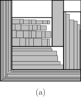
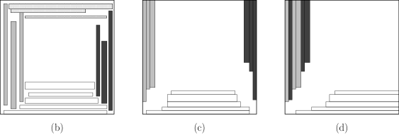
Figure 4.1: (a) An L&C-packing with $4$ containers, where the top-left container is packed by means of Next-Fit-Decreasing-Height. (b) A subset of long items. (c) Such items are shifted into $4$ stacks at the sides of the knapsack, and the top stack is deleted. (d) The final packing into an L-shaped region.

For weighted 2DGK we face severe technical complications for proving that there is a profitable L&C-packing. One key reason is that in the weighted case we cannot discard large items since even one such item might contribute a large fraction to the optimal profit.

In order to circumvent these difficulties, we exploit the corridor-partition at the heart of the QPTAS for 2DGK in Adamaszek and Wiese [2015] (in turn inspired by prior work in Adamaszek and Wiese [2013]). Roughly speaking, there exists a partition of the knapsack into $O_{\varepsilon}(1)$ corridors, consisting of the concatenation of $O_{\varepsilon}(1)$ (partially overlapping) rectangular regions (subcorridors).

In Adamaszek and Wiese [2015] the authors partition the corridors into a poly-logarithmic number of containers. Their main algorithm then guesses these containers in time $n^{\operatorname{poly\,log}n}$. However, we can only handle a constant number of containers in polynomial time. Therefore, we present a different way to partition the corridors into containers: here we lose the profit of a set of thin items, which in some sense play the role of long items in the previous discussion. These thin items fit in a very narrow ring at the boundary of the knapsack and we map them to an L-packing in the same way as in the cardinality case above. Some of the remaining non-thin items are then packed into $O_{\varepsilon}(1)$ containers that are placed in the (large) part of the knapsack not occupied by the L-packing. Our partition of the corridors is based on a somewhat intricate case analysis that exploits the fact that long consecutive subcorridors are arranged in the shape of rings or spirals: this is used to show the existence of a profitable L&C-packing.

Theorem 36.

There is a polynomial-time $\frac{17}{9}+\varepsilon<1.89$ approximation algorithm for (weighted) 2DGK.

4.1 A PTAS for L-packings

In this section we present a PTAS for the problem of finding an optimal L-packing. In this problem we are given a set of horizontal items $I_{hor}$ with width larger than $N/2$, and a set of vertical items $I_{ver}$ with height larger than $N/2$. Furthermore, we are given an L-shaped region $L=([0,N]\times[0,0pt_{L}])\cup([0,0pt_{L}]\times[0,N])$. Our goal is to pack a subset $OPT\subseteq I:=I_{hor}\cup I_{ver}$ of maximum total profit $opt=p(OPT):=\sum_{i\in OPT}p(i)$, such that $OPT_{hor}:=OPT\cap I_{hor}$ is packed inside the horizontal box $[0,N]\times[0,0pt_{L}]$ and $OPT_{ver}:=OPT\cap I_{ver}$ is packed inside the vertical box $[0,0pt_{L}]\times[0,N]$. We remark that packing horizontal and vertical items independently is not possible due to the possible overlaps in the intersection of the two boxes: this is what makes this problem non-trivial, in particular harder than standard (one-dimensional) knapsack.

Observe that in an optimal packing we can assume without loss of generality that items in $OPT_{hor}$ are pushed as far to the right/bottom as possible: indeed pushing one such item to the right/bottom keeps the packing feasible. Furthermore, the items in $OPT_{hor}$ are packed from bottom to top in non-increasing order of width. Indeed, it is possible to permute any two items violating this property while keeping the packing feasible. A symmetric claim holds for $OPT_{ver}$. See Figure 4.1.(d) for an illustration.

Given the above structure, it is relatively easy to define a dynamic program (DP) that computes an optimal L-packing in pseudo-polynomial time $(Nn)^{O(1)}$. The basic idea is to scan items of $I_{hor}$ (resp. $I_{ver}$) in decreasing order of width (resp. height), and each time guess if they are part of the optimal solution $OPT$. At each step either both the considered horizontal item $i$ and vertical item $j$ are not part of the optimal solution, or there exist a guillotine cut separating $i$ or $j$ from the rest of $OPT$. Depending on the cases, one can define a smaller L-packing sub-instance (among $N^{2}$ choices) for which the DP table already contains a solution.

In order to achieve a $(1+\varepsilon)$-approximation in polynomial time $n^{O_{\varepsilon}(1)}$, we show that it is possible (with a small loss in the profit) to restrict the possible top coordinates of $OPT_{hor}$ and right coordinates of $OPT_{ver}$ to proper polynomial-size subsets ${\cal T}$ and ${\cal R}$, resp. We call such an L-packing $({\cal T},{\cal R})$-restricted. By adapting the above DP one obtains:

Lemma 37.

An optimal $({\cal T},{\cal R})$-restricted L-packing can be computed in time polynomial in $m:=n+|{\cal T}|+|{\cal R}|$ using dynamic programming.

Proof.

For notational convenience we assume $0\in{\cal T}$ and $0\in{\cal R}$. Let $h_{1},\ldots,h_{n(h)}$ be the items in $I_{hor}$ in decreasing order of width and $v_{1},\ldots,v_{n(v)}$ be the items in $I_{ver}$ in decreasing order of height (breaking ties arbitrarily). For $0pt\in[0,0pt_{L}]$ and $0pt\in[0,0pt_{L}]$, let $L(0pt,0pt)=([0,0pt]\times[0,N])\cup([0,N]\times[0,0pt])\subseteq L$. Let also $\Delta L(0pt,0pt)=([0pt,0pt_{L}]\times[0pt,N])\cup([0pt,N]\times[0pt,0pt_{L}])\subseteq L$. Note that $L=L(0pt,0pt)\cup\Delta L(0pt,0pt)$.

We define a dynamic program table $DP$ indexed by $i\in[1,n(h)]$ and $j\in[1,n(v)]$, by a top coordinate $t\in{\cal T}$, and a right coordinate $r\in{\cal R}$. The value of $DP(i,t,j,r)$ is the maximum profit of a $({\cal T},{\cal R})$-restricted packing of a subset of $\{h_{i},\ldots,h_{n(h)}\}\cup\{v_{j},\ldots,v_{n(v)}\}$ inside $\Delta L(r,t)$. The value of $DP(1,0,1,0)$ is the value of the optimum solution we are searching for. Note that the number of table entries is upper bounded by $m^{4}$.

We fill in $DP$ according to the partial order induced by vectors $(i,t,j,r)$, processing larger vectors first. The base cases are given by $(i,j)=(n(h)+1,n(v)+1)$ and $(r,t)=(0pt_{L},0pt_{L})$, in which case the table entry has value $0$.

In order to compute any other table entry $DP(i,t,j,r)$, with optimal solution $OPT^{\prime}$, we take the maximum of the following few values:

• If $i\leq n(h)$, the value $DP(i+1,t,j,r)$. This covers the case that $h_{i}\notin OPT^{\prime}$;

• If $j\leq n(v)$, the value $DP(i,t,j+1,r)$. This covers the case that $v_{j}\notin OPT^{\prime}$;

• Assume that there exists $t^{\prime}\in{\cal T}$ such that $t^{\prime}-0pt(h_{i})\geq t$ and that $0pt(h_{i})\leq N-r$. Then for the minimum such $t^{\prime}$ we consider the value $p(h_{i})+DP(i+1,t^{\prime},j,r)$. This covers the case that $h_{i}\in OPT^{\prime}$, and there exists a (horizontal) guillotine cut separating $h_{i}$ from $OPT^{\prime}\setminus\{h_{i}\}$.

• Assume that there exists $r^{\prime}\in{\cal R}$ such that $r^{\prime}-0pt(v_{j})\geq r$ and that $0pt(v_{j})\leq N-t$. Then for the minimum such $r^{\prime}$ we consider the value $p(v_{j})+DP(i,t,j+1,r^{\prime})$. This covers the case that $v_{j}\in OPT^{\prime}$, and there exists a (vertical) guillotine cut separating $v_{j}$ from $OPT^{\prime}\setminus\{v_{j}\}$.

We observe that the above cases (which can be explored in polynomial time) cover all the possible configurations in $OPT^{\prime}$. Indeed, if the first two cases do not apply, we have that $h_{i},v_{j}\in OPT^{\prime}$. Then either the line containing the right side of $v_{j}$ does not intersect $h_{i}$ (hence any other item in $OPT^{\prime}$) or the line containing the top side of $h_{i}$ does not intersect $v_{j}$ (hence any other item in $OPT^{\prime}$). Indeed, the only remaining case is that $v_{j}$ and $h_{i}$ overlap, which is impossible since they both belong to $OPT^{\prime}$. ∎

We will show that there exists a $({\cal T},{\cal R})$-restricted L-packing with the desired properties.

Lemma 38.

There exists an $({\cal T},{\cal R})$-restricted L-packing solution of profit at least $(1-2\varepsilon)opt$, where the sets ${\cal T}$ and ${\cal R}$ have cardinality at most $n^{O(1/\varepsilon^{1/\varepsilon})}$ and can be computed in polynomial time based on the input (without knowing $OPT$).

Lemmas 37 and 38, together immediately imply a PTAS for L-packings (showing Theorem 34). The rest of this section is devoted to the proof of Lemma 38.

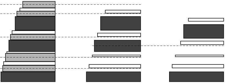
Figure 4.2: Illustration of the delete&shift procedure with $r_{hor}=2$. The dashed lines indicate the value of the new baselines in the different stages of the algorithm. (Left) The starting packing. Dark and light gray items denote the growing sequences for the calls with $r=2$ and $r=1$, resp. (Middle) The shift of items at the end of the recursive calls with $r=1$. Note that light gray items are all deleted, and dark gray items are not shifted. (Right) The shift of items at the end of the process. Here we assume that the middle dark gray item is deleted.

We will describe a way to delete a subset of items $D_{hor}\subseteq OPT_{hor}$ with $p(D_{hor})\leq 2\varepsilon p(OPT_{hor})$, and shift down the remaining items $OPT_{hor}\setminus D_{hor}$ so that their top coordinate belongs to a set ${\cal T}$ with the desired properties. Symmetrically, we will delete a subset of items $D_{ver}\subseteq OPT_{ver}$ with $p(D_{ver})\leq 2\varepsilon p(OPT_{ver})$, and shift to the left the remaining items $OPT_{ver}\setminus D_{ver}$ so that their right coordinate belongs to a set ${\cal R}$ with the desired properties. We remark that shifting down (resp. to the left) items of $OPT_{hor}$ (resp. $OPT_{ver}$) cannot create any overlap with items of $OPT_{ver}$ (resp. $OPT_{hor}$). This allows us to reason on each such set separately.

We next focus on $OPT_{hor}$ only: the construction for $OPT_{ver}$ is symmetric. For notational convenience we let $1,\ldots,n_{hor}$ be the items of $OPT_{hor}$ in non-increasing order of width and from bottom to top in the starting optimal packing. We remark that this sequence is not necessarily sorted (increasingly or decreasingly) in terms of item heights: this makes our construction much more complicated.

Let us first introduce some useful notation. Consider any subsequence $B=\{b_{start},\ldots,b_{end}\}$ of consecutive items (interval). For any $i\in B$, we define $top_{B}(i):=\sum_{k\in B,k\leq i}0pt(k)$ and $bottom_{B}(i)=top_{B}(i)-0pt(i)$. The growing subsequence $G=G(B)=\{g_{1},\ldots,g_{h}\}$ of $B$ (with possibly non-contiguous elements) is defined as follows. We initially set $g_{1}=b_{start}$. Given the element $g_{i}$, $g_{i+1}$ is the smallest-index (i.e., lowest) element in $\{g_{i}+1,\ldots,b_{end}\}$ such that $0pt(g_{i+1})\geq 0pt(g_{i})$. We halt the construction of $G$ when we cannot find a proper $g_{i+1}$. For notational convenience, define $g_{h+1}=b_{end}+1$. We let $B^{G}_{i}:=\{g_{i}+1,\ldots,g_{i+1}-1\}$ for $i=1,\ldots,h$. Observe that the sets $B^{G}_{i}$ partition $B\setminus G$. We will crucially exploit the following simple property.

Lemma 39.

For any $g_{i}\in G$ and any $j\in\{b_{start},\ldots,g_{i+1}-1\}$, $0pt(j)\leq 0pt(g_{i})$.

Proof.

The items $j\in B^{G}_{i}=\{g_{i}+1,\ldots,g_{i+1}-1\}$ have $0pt(j)<0pt(g_{i})$. Indeed, any such $j$ with $0pt(j)\geq 0pt(g_{i})$ would have been added to $G$, a contradiction.

Consider next any $j\in\{b_{start},\ldots g_{i}-1\}$. If $j\in G$ the claim is trivially true by construction of $G$. Otherwise, one has $j\in B^{G}_{k}$ for some $g_{k}\in G$, $g_{k}<g_{i}$. Hence, by the previous argument and by construction of $G$, $0pt(j)<0pt(g_{k})\leq 0pt(g_{i})$. ∎

The intuition behind our construction is as follows. Consider the growing sequence $G=G(OPT_{hor})$, and suppose that $p(G)\leq\varepsilon\cdot p(OPT_{hor})$. Then we might simply delete $G$, and shift the remaining items $OPT_{hor}\setminus G=\cup_{j}B^{G}_{j}$ as follows. Let $\lceil x\rceil_{y}$ denote the smallest multiple of $y$ not smaller than $x$. We consider each set $B^{G}_{j}$ separately. For each such set, we define a baseline vertical coordinate $base_{j}=\lceil bottom(g_{j})\rceil_{0pt(g_{j})/2}$, where $bottom(g_{j})$ is the bottom coordinate of $g_{j}$ in the original packing. We next round up the height of $i\in B^{G}_{j}$ to $\hat{0pt}(i):=\lceil 0pt(i)\rceil_{0pt(g_{j})/(2n)}$, and pack the rounded items of $B^{G}_{j}$ as low as possible above the baseline. The reader might check that the possible top coordinates for rounded items fall in a polynomial size set (using Lemma 39). It is also not hard to check that items are not shifted up.

We use recursion in order to handle the case $p(G)>\varepsilon\cdot p(OPT_{hor})$. Rather than deleting $G$, we consider each $B^{G}_{j}$ and build a new growing subsequence for each such set. We repeat the process recursively for $r_{hor}$ many rounds. Let ${\cal G}^{r}$ be the union of all the growing subsequences in the recursive calls of level $r$. Since the sets ${\cal G}^{r}$ are disjoint by construction, there must exist a value $r_{hor}\leq\frac{1}{\varepsilon}$ such that $p({\cal G}^{r_{hor}})\leq\varepsilon\cdot p(OPT_{hor})$. Therefore we can apply the same shifting argument to all growing subsequences of level $r_{hor}$ (in particular we delete all of them). In the remaining growing subsequences we can afford to delete $1$ out of $1/\varepsilon$ consecutive items (with a small loss of the profit), and then apply a similar shifting argument.

We next describe our approach in more detail. We exploit a recursive procedure delete&shift. This procedure takes in input two parameters: an interval $B=\{b_{start},\ldots,b_{end}\}$, and an integer round parameter $r\geq 1$. Procedure delete&shift returns a set $D(B)\subseteq B$ of deleted items, and a shift function $shift:B\setminus D(B)\rightarrow\mathbb{N}$. Intuitively, $shift(i)$ is the value of the top coordinate of $i$ in the shifted packing with respect to a proper baseline value which is implicitly defined. We initially call delete&shift$(OPT_{hor},r_{hor})$, for a proper $r_{hor}\in\{1,\ldots,\frac{1}{\varepsilon}\}$ to be fixed later. Let $(D,shift)$ be the output of this call. The desired set of deleted items is $D_{hor}=D$, and in the final packing $top(i)=shift(i)$ for any $i\in OPT_{hor}\setminus D_{hor}$ (the right coordinate of any such $i$ is $N$).

The procedure behaves differently in the cases $r=1$ and $r>1$. If $r=1$, we compute the growing sequence $G=G(B)=\{g_{1}=b_{start},\ldots,g_{h}\}$, and set $D(B)=G(B)$. Considers any set $B^{G}_{j}=\{g_{j}+1,\ldots,g_{j+1}-1\}$, $j=1,\ldots,h$. Let $base_{j}:=\lceil bottom_{B}(g_{j})\rceil_{0pt(g_{j})/2}$. We define for any $i\in B^{G}_{j}$,

$$shift(i)=base_{j}+\sum_{k\in B^{G}_{j},k\leq i}\lceil 0pt(k)\rceil_{0pt(g_{j})/(2n)}.$$

Observe that $shift$ is fully defined since $\cup_{j=1}^{h}B^{G}_{j}=B\setminus D(B)$.

If instead $r>1$, we compute the growing sequence $G=G(B)=\{g_{1}=b_{start},\ldots,g_{h}\}$. We next delete a subset of items $D^{\prime}\subseteq G$. If $h<\frac{1}{\varepsilon}$, we let $D^{\prime}=D^{\prime}(B)=\emptyset$. Otherwise, let $G_{k}=\{g_{j}\in G:j=k\pmod{1/\varepsilon}\}\subseteq G$, for $k\in\{0,\ldots,1/\varepsilon-1\}$. We set $D^{\prime}=D^{\prime}(B)=\{d_{1},\ldots,d_{p}\}=G_{x}$ where $x=\arg\min_{k\in\{0,\ldots,1/\varepsilon-1\}}p(G_{k})$.

Proposition 40.

One has $p(D^{\prime})\leq\varepsilon\cdot p(G)$. Furthermore, any subsequence $\{g_{x},g_{x+1},\ldots,g_{y}\}$ of $G$ with at least $1/\varepsilon$ items contains at least one item from $D^{\prime}$.

Consider each set $B^{G}_{j}=\{g_{j}+1,\ldots,g_{j+1}-1\}$, $j=1,\ldots,h$: We run delete&shift$(B^{G}_{j},r-1)$. Let $(D_{j},shift_{j})$ be the output of the latter procedure, and $shift^{max}_{j}$ be the maximum value of $shift_{j}$. We set the output set of deleted items to $D(B)=D^{\prime}\cup(\cup_{j=1}^{h}D_{j})$.

It remains to define the function $shift$. Consider any set $B^{G}_{j}$, and let $d_{q}$ be the deleted item in $D^{\prime}$ with largest index (hence in topmost position) in $\{b_{start},\ldots,g_{j}\}$: define $base_{q}=\lceil bottom_{B}(d_{q})\rceil_{0pt(d_{q})/2}$. If there is no such $d_{q}$, we let $d_{q}=0$ and $base_{q}=0$. For any $i\in B^{G}_{j}$ we set:

$$shift(i)=base_{q}+\sum_{g_{k}\in G,d_{q}<g_{k}\leq g_{j}}0pt(g_{k})+\sum_{g_{k}\in G,d_{q}\leq g_{k}<g_{j}}shift^{max}_{k}+shift_{j}(i).$$

Analogously, if $g_{j}\neq d_{q}$, we set

$$shift(g_{j})=base_{q}+\sum_{g_{k}\in G,d_{q}<g_{k}\leq g_{j}}0pt(g_{k})+\sum_{g_{k}\in G,d_{q}\leq g_{k}<g_{j}}shift^{max}_{k}.$$

This concludes the description of delete&shift. We next show that the final packing has the desired properties. Next lemma shows that the total profit of deleted items is small for a proper choice of the starting round parameter $r_{hor}$.

Lemma 41.

There is a choice of $r_{hor}\in\{1,\ldots,\frac{1}{\varepsilon}\}$ such that the final set $D_{hor}$ of deleted items satisfies $p(D_{hor})\leq 2\varepsilon\cdot p(OPT_{hor})$.

Proof.

Let ${\cal G}^{r}$ denote the union of the sets $G(B)$ computed by all the recursive calls with input round parameter $r$. Observe that by construction these sets are disjoint. Let also ${\cal D}^{r}$ be the union of the sets $D^{\prime}(B)$ on those calls (the union of sets $D(B)$ for $r=r_{hor}$). By Proposition 40 and the disjointness of sets ${\cal G}^{r}$ one has

$$p(D_{hor})=\sum_{1\leq r\leq r_{hor}}p({\cal D}^{r})\leq\varepsilon\cdot\sum_{r<r_{hor}}p({\cal G}^{r})+p({\cal D}^{r_{hor}})\leq\varepsilon\cdot p(OPT_{hor})+p({\cal D}^{r_{hor}}).$$

Again by the disjointness of sets ${\cal G}^{r}$ (hence ${\cal D}^{r}$), there must exists a value of $r_{hor}\in\{1,\ldots,\frac{1}{\varepsilon}\}$ such that $p({\cal D}^{r_{hor}})\leq\varepsilon\cdot p(OPT_{hor})$. The claim follows. ∎

Next lemma shows that, intuitively, items are only shifted down with respect to the initial packing.

Lemma 42.

Let $(D,shift)$ be the output of some execution of the algorithm delete&shift$(B,r)$. Then, for any $i\in B\setminus D$, $shift(i)\leq top_{B}(i)$.

Proof.

We prove the claim by induction on $r$. Consider first the case $r=1$. In this case, for any $i\in B^{G}_{j}$:

$$shift(i) =\lceil bottom_{B}(g_{j})\rceil_{0pt(g_{j})/2}+\sum_{k\in B^{G}_{j},k\leq i}\lceil 0pt(k)\rceil_{0pt(g_{j})/(2n)}$$

$$\leq top_{B}(g_{j})-\frac{1}{2}0pt(g_{j})+\sum_{k\in B^{G}_{j},k\leq i}0pt(k)+n\cdot\frac{0pt(g_{j})}{2n}=top_{B}(i).$$

Assume next that the claim holds up to round parameter $r-1\geq 1$, and consider round $r$. For any $i\in B^{G}_{j}$ with $base_{q}=\lceil bottom_{B}(d_{q})\rceil_{0pt(d_{q})/2}$, one has

$$shift(i) =\lceil bottom_{B}(d_{q})\rceil_{0pt(d_{q})/2}+\sum_{\begin{subarray}{c}g_{k}\in G,\\ d_{q}<g_{k}\leq g_{j}\end{subarray}}0pt(g_{k})+\sum_{\begin{subarray}{c}g_{k}\in G,\\ d_{q}\leq g_{k}<g_{j}\end{subarray}}shift^{max}_{k}+shift_{j}(i)$$

$$\leq top_{B}(d_{q})+\sum_{\begin{subarray}{c}g_{k}\in G,\\ d_{q}<g_{k}\leq g_{j}\end{subarray}}0pt(g_{k})+\sum_{\begin{subarray}{c}g_{k}\in G,\\ d_{q}\leq g_{k}<g_{j}\end{subarray}}top_{B^{G}_{k}}(g_{k+1}-1)+top_{B^{G}_{j}}(i)$$

$$=top_{B}(i).$$

An analogous chain of inequalities shows that $shift(g_{j})\leq top_{B}(g_{j})$ for any $g_{j}\in G\setminus D^{\prime}$. A similar proof works for the special case $base_{q}=0$. ∎

It remains to show that the final set of values of $top(i)=shift(i)$ has the desired properties. This is the most delicate part of our analysis. We define a set ${\cal T}^{r}$ of candidate top coordinates recursively in $r$. Set ${\cal T}^{1}$ contains, for any item $j\in I_{hor}$, and any integer $1\leq a\leq 4n^{2}$, the value $a\cdot\frac{0pt(j)}{2n}$. Set ${\cal T}^{r}$, for $r>1$ is defined recursively with respect to to ${\cal T}^{r-1}$. For any item $j$, any integer $0\leq a\leq 2n-1$, any tuple of $b\leq 1/\varepsilon-1$ items $j(1),\ldots,j(b)$, and any tuple of $c\leq 1/\varepsilon$ values $s(1),\ldots,s(c)\in{\cal T}^{r-1}$, ${\cal T}^{r}$ contains the sum $a\cdot\frac{0pt(j)}{2}+\sum_{k=1}^{b}0pt(j(k))+\sum_{k=1}^{c}s(k)$. Note that sets ${\cal T}^{r}$ can be computed based on the input only (without knowing $OPT$). It is easy to show that ${\cal T}^{r}$ has polynomial size for $r=O_{\varepsilon}(1)$.

Lemma 43.

For any integer $r\geq 1$, $|{\cal T}^{r}|\leq(2n)^{\frac{r+2+(r-1)\varepsilon}{\varepsilon^{r-1}}}$.

Proof.

We prove the claim by induction on $r$. The claim is trivially true for $r=1$ since there are $n$ choices for item $j$ and $4n^{2}$ choices for the integer $a$, hence altogether at most $n\cdot 4n^{2}<8n^{3}$ choices. For $r>1$, the number of possible values of ${\cal T}^{r}$ is at most

$$n\cdot 2n\cdot\left(\sum_{b=0}^{1/\varepsilon-1}n^{b}\right)\cdot\left(\sum_{c=0}^{1/\varepsilon}|{\cal T}^{r-1}|^{c}\right) \leq 4n^{2}\cdot n^{\frac{1}{\varepsilon}-1}\cdot|{\cal T}^{r-1}|^{\frac{1}{\varepsilon}}$$

$$\leq(2n)^{\frac{1}{\varepsilon}+1}\left((2n)^{\frac{r+1+(r-2)\varepsilon}{\varepsilon^{r-2}}}\right)^{\frac{1}{\varepsilon}}$$

$$\leq(2n)^{\frac{r+2+(r-1)\varepsilon}{\varepsilon^{r-1}}}.$$

∎

The next lemma shows that the values of $shift$ returned by delete&shift for round parameter $r$ belong to ${\cal T}^{r}$, hence the final top coordinates belong to ${\cal T}:={\cal T}^{r_{hor}}$.

Lemma 44.

Let $(D,shift)$ be the output of some execution of the procedure delete&shift$(B,r)$. Then, for any $i\in B\setminus D$, $shift(i)\in{\cal T}^{r}$.

Proof.

We prove the claim by induction on $r$. For the case $r=1$, recall that for any $i\in B^{G}_{j}$ one has

$$shift(i) =\lceil bottom_{B}(g_{j})\rceil_{0pt(g_{j})/2}+\sum_{k\in B^{G}_{j},k\leq i}\lceil 0pt(k)\rceil_{0pt(g_{j})/(2n)}.$$

By Lemma 39, $bottom_{B}(g_{j})=\sum_{k\in B,k<g_{j}}0pt(k)\leq(n-1)\cdot 0pt(g_{j})$. By the same lemma, $\sum_{k\in B^{G}_{j},k\leq i}0pt(k)\leq(n-1)\cdot 0pt(g_{j})$. It follows that

$$shift(i)\leq 2(n-1)\cdot 0pt(g_{j})+\frac{0pt(g_{j})}{2}+(n-1)\cdot\frac{0pt(g_{j})}{2n}\leq 4n^{2}\cdot\frac{0pt(g_{j})}{2n}.$$

Hence $shift(i)=a\cdot\frac{0pt(g_{j})}{2n}$ for some integer $1\leq a\leq 4n^{2}$, and $shift(i)\in{\cal T}^{1}$ for $j=g_{j}$ and for a proper choice of $a$.

Assume next that the claim is true up to $r-1\geq 1$, and consider the case $r$. Consider any $i\in B^{G}_{j}$, and assume $0<base_{q}=\lceil bottom_{B}(d_{q})\rceil_{0pt(d_{q})/2}$. One has:

$$shift(i) =\lceil bottom_{B}(d_{q})\rceil_{0pt(d_{q})/2}+\sum_{\begin{subarray}{c}g_{k}\in G,\\ d_{q}<g_{k}\leq g_{j}\end{subarray}}0pt(g_{k})+\sum_{\begin{subarray}{c}g_{k}\in G,\\ d_{q}\leq g_{k}<g_{j}\end{subarray}}shift^{max}_{k}+shift_{j}(i).$$

By Lemma 39, $bottom_{B}(d_{q})\leq(n-1)0pt(d_{q})$, therefore $\lceil bottom_{B}(d_{q})\rceil_{0pt(d_{q})/2}=a\cdot\frac{0pt(d_{q})}{2}$ for some integer $1\leq a\leq 2(n-1)+1$. By Proposition 40, $|\{g_{k}\in G,d_{q}<g_{k}\leq g_{j}\}|\leq 1/\varepsilon-1$. Hence $\sum_{g_{k}\in G,d_{q}<g_{k}\leq g_{j}}0pt(g_{k})$ is a value contained in the set of sums of $b\leq 1/\varepsilon-1$ item heights. By inductive hypothesis $shift^{max}_{k},shift_{j}(i)\in{\cal T}^{r-1}$. Hence by a similar argument the value of $\sum_{g_{k}\in G,d_{q}\leq g_{k}<g_{j}}shift^{max}_{k}+shift_{j}(i)$ is contained in the set of sums of $c\leq 1/\varepsilon-1+1$ values taken from ${\cal T}^{r-1}$. Altogether, $shift(i)\in{\cal T}^{r}$. A similar argument, without the term $shift_{j}(i)$, shows that $shift(g_{j})\in{\cal T}^{r}$ for any $g_{j}\in G\setminus D^{\prime}$. The proof works similarly in the case $base_{q}=0$ by setting $a=0$. The claim follows. ∎

Proof of Lemma 38.

We apply the procedure deleted&shift to $OPT_{hor}$ as described before, and a symmetric procedure to $OPT_{ver}$. In particular the latter procedure computes a set $D_{ver}\subseteq OPT_{ver}$ of deleted items, and the remaining items are shifted to the left so that their right coordinate belongs to a set ${\cal R}:={\cal R}^{r_{ver}}$, defined analogously to the case of ${\cal T}:={\cal T}^{r_{hor}}$, for some integer $r_{ver}\in\{1,\ldots,1/\varepsilon\}$ (possibly different from $r_{hor}$, though by averaging this is not critical).

It is easy to see that the profit of non-deleted items satisfies the claim by Lemma 41 and its symmetric version. Similarly, the sets ${\cal T}$ and ${\cal R}$ satisfy the claim by Lemmas 43 and 44, and their symmetric versions. Finally, with respect to the original packing non-deleted items in $OPT_{hor}$ and $OPT_{ver}$ can be only shifted to the bottom and to the left, resp. by Lemma 42 and its symmetric version. This implies that the overall packing is feasible.∎

4.2 A Simple Improved Approximation for Cardinality 2DGK

In this section we present a simple improved approximation for the cardinality case of 2DGK. We can assume that the optimal solution $OPT\subseteq I$ satisfies that $|OPT|\geq 1/\varepsilon^{3}$ since otherwise we can solve the problem optimally by brute force in time $n^{O(1/\varepsilon^{3})}$. Therefore, we can discard from the input all large items with both sides larger than $\varepsilon\cdot N$: any feasible solution can contain at most $1/\varepsilon^{2}$ such items, and discarding them decreases the cardinality of $OPT$ at most by a factor $1+\varepsilon$. Let $OPT$ denote this slightly sub-optimal solution obtained by removing large items.

We will need the following technical lemma, which also works unchanged for the weighted case. See also Figure 4.1.(b)–(d).

Lemma 45.

Let $H$ and $V$ be given subsets of items from some feasible solution with width and height strictly larger than $N/2$, resp. Let $0pt_{H}$ and $0pt_{V}$ be the total height and width of items of $H$ and $V$, resp. Then there exists an $L$-packing of a set $APX\subseteq H\cup V$ with $p(APX)\geq\frac{3}{4}(p(H)+p(V))$ into the area $L=([0,N]\times[0,0pt_{H}])\cup([0,0pt_{V}]\times[0,N])$.

Proof.

Let us consider the packing of $H\cup V$. Consider each $i\in H$ that has no $j\in V$ to its top (resp. to its bottom) and shift it up (resp. down) until it hits another $i^{\prime}\in H$ or the top (resp, bottom) side of the knapsack. Note that, since $0pt(j)>N/2$ for any $j\in V$, one of the two cases above always applies. We iterate this process as long as it is possible to move any such $i$. We perform a symmetric process on $V$. At the end of the process all items in $H\cup V$ are stacked on the $4$ sides of the knapsack.

Next we remove the least profitable of the $4$ stacks: by a simple permutation argument we can guarantee that this is the top or right stack. We next discuss the case that it is the top one, the other case being symmetric. We show how to repack the remaining items in a boundary $L$ of the desired size by permuting items in a proper order. In more detail, suppose that the items packed on the left (resp. right and bottom) have a total width of $0pt_{l}$ (resp. total width of $0pt_{r}$ and total height of $0pt_{b}$). We next show that there exists a packing into $L^{\prime}=([0,N]\times[0,0pt_{b}])\cup([0,0pt_{l}+0pt_{r}]\times[0,N])$. We prove the claim by induction. Suppose that we have proved it for all packings into left, right and bottom stacks with parameters $0pt^{\prime}_{l}$, $0pt^{\prime}_{r}$, and $0pt^{\prime}$ such that $0pt^{\prime}<0pt_{b}$ or $0pt^{\prime}_{l}+0pt^{\prime}_{r}<0pt_{l}+0pt_{r}$ or $0pt^{\prime}_{l}+0pt^{\prime}_{r}=0pt_{l}+0pt_{r}$ and $0pt^{\prime}_{r}<0pt_{r}$.

In the considered packing we can always find a guillotine cut $\ell$, such that one side of the cut contains precisely one lonely item among the leftmost, rightmost and bottommost items. Let $\ell$ be such a cut. First assume that the lonely item $j$ is the bottommost one. Then by induction the claim is true for the part above $\ell$ since the part of the packing above $\ell$ has parameters $0pt_{l},0pt_{r}$, and $0pt-0pt(j)$. Thus, it is also true for the entire packing. A similar argument applies if the lonely item $j$ is the leftmost one.

It remains to consider the case that the lonely item $j$ is the rightmost one. We remove $j$ temporarily and move all other items by $0pt(j)$ to the right. Then we insert $j$ at the left (in the space freed by the previous shifting). By induction, the claim is true for the resulting packing since it has parameters $0pt_{l}+0pt(j)$, $0pt_{r}-0pt(j)$, and $0pt$, resp. ∎

For our algorithm, we consider the following three packings. The first uses an $L$ that occupies the full knapsack, i.e., $0pt_{L}=0pt_{L}=N$. Let $OPT_{long}\subseteq OPT$ be the items in $OPT$ with height or width strictly larger than $N/2$ and define $OPT_{short}=OPT\setminus OPT_{long}$. We apply Lemma 45 to $OPT_{long}$ and hence obtain a packing for this $L$ with a profit of at least $\frac{3}{4}w(OPT_{long})$. We run our PTAS for L-packings from Theorem 34 on this L, the input consisting of all items in $I$ having one side longer than $N/2$. Hence we obtain a solution with profit at least $(\frac{3}{4}-O(\varepsilon))w(OPT_{long})$.

For the other two packings we employ the one-sided resource augmentation PTAS given from Lemma 14 and Theorem 12. We apply this algorithm to the slightly reduced knapsacks $[0,N]\times[0,N/(1+\varepsilon)]$ and $[0,N/(1+\varepsilon)]\times[0,N]$ such that in both cases it outputs a solution that fits in the full knapsack $[0,N]\times[0,N]$ and whose profit is by at most a factor $1+O(\varepsilon)$ worse than the optimal solution for the respective reduced knapsacks. Will prove in Theorem 46 that one of these solutions yields a profit of at least $(\frac{1}{2}-O(\varepsilon))p(OPT)+(\frac{1}{4}-O(\varepsilon))p(OPT_{short})$ and hence one of our packings yields a $(\frac{16}{9}+\varepsilon)$-approximation.

Theorem 46.

There is a $\left(\frac{16}{9}+\varepsilon\right)$-approximation for the cardinality case of 2DGK.

Proof.

Let $OPT$ be the considered optimal solution with $opt=p(OPT)$. Recall that there are no large items. Let also $OPT_{vert}\subseteq OPT$ be the (vertical) items with height more than $\varepsilon\cdot N$ (hence with width at most $\varepsilon\cdot N$), and $OPT_{hor}=OPT\setminus OPT_{ver}$ (horizontal items). Note that with this definition both sides of a horizontal item might have a length of at most $\varepsilon\cdot N$. We let $opt_{long}=p(OPT_{long})$ and $opt_{short}=p(OPT_{short})$.

As mentioned above, our $L$-packing PTAS achieves a profit of at least $(\frac{3}{4}-O(\varepsilon))opt_{long}$ which can be seen by applying Lemma 45 with $H=OPT_{long}\cap OPT_{hor}$ and $V=OPT_{long}\cap OPT_{ver}$. In order to show that the other two packings yield a good profit, consider a random horizontal strip $S=[0,N]\times[a,a+\varepsilon\cdot N]$ (fully contained in the knapsack) where $a\in[0,(1-\varepsilon)N)$ is chosen uniformly at random. We remove all items of $OPT$ intersecting $S$. Each item in $OPT_{hor}$ and $OPT_{short}\cap OPT_{ver}$ is deleted with probability at most $3\varepsilon$ and $\frac{1}{2}+2\varepsilon$, resp. Therefore the total profit of the remaining items is in expectation at least $(1-3\varepsilon)p(OPT_{hor})+(\frac{1}{2}-2\varepsilon)p(OPT_{short}\cap OPT_{vert})$. Observe that the resulting solution can be packed into a restricted knapsack of size $[0,N]\times[0,N/(1+\varepsilon)]$ by shifting down the items above the horizontal strip. Therefore, when we apply the resource augmentation algorithm in Jansen and Solis-Oba [2007] to the knapsack $[0,N]\times[0,N/(1+\varepsilon)]$, up to a factor $1-\varepsilon$, we will find a solution of (deterministically!) at least the same profit. In other terms, this profit is at least $(1-4\varepsilon)p(OPT_{hor})+(\frac{1}{2}-\frac{5}{2}\varepsilon)p(OPT_{short}\cap OPT_{vert})$.

By a symmetric argument, we obtain a solution of profit at least $(1-4\varepsilon)p(OPT_{ver})+(\frac{1}{2}-\frac{5}{2}\varepsilon)p(OPT_{short}\cap OPT_{hor})$ when we apply the algorithm in Jansen and Solis-Oba [2007] to the knapsack $[0,N/(1+\varepsilon)]\times[0,N]$. Thus the best of the latter two solutions has profit at least $(\frac{1}{2}-2\varepsilon)opt_{long}+(\frac{3}{4}-\frac{13}{4}\varepsilon)opt_{short}=(\frac{1}{2}-2\varepsilon)opt+(\frac{1}{4}-\frac{5}{4}\varepsilon)opt_{short}$. The best of our three solutions has therefore value at least $(\frac{9}{16}-O(\varepsilon))opt$ where the worst case is achieved for roughly $opt_{long}=3\cdot opt_{short}$. ∎

4.3 Weighted Case Without Rotations

In this section we show how to extend the reasoning of the unweighted case to the weighted case. This requires much more complicated technical machinery than the algorithm presented in Section 4.2.

Our strategy is to start with a partition of the knapsack into thin corridors as defined in Adamaszek and Wiese [2015]. Then, we partition these corridors into a set of rectangular boxes and an L-packing. We first present a simplified version of our argumentation in which we assume that we are allowed to drop $O_{\varepsilon}(1)$ many items at no cost, i.e., we pretend that we have the right to remove $O_{\varepsilon}(1)$ items from $OPT$ and compare the profit of our computed solution with the remaining set. Building on this, we give an argumentation for the general case which will involve some additional shifting arguments.

4.3.1 Item classification

We start with a classification of the input items according to their heights and widths. For two given constants $1\geq\varepsilon_{large}>\varepsilon_{small}>0$, we classify an item $i$ as:

• small if $h_{i},w_{i}\leq\varepsilon_{small}N$;

• large if $h_{i},w_{i}>\varepsilon_{large}N$;

• horizontal if $w_{i}>\varepsilon_{large}N$ and $h_{i}\leq\varepsilon_{small}N$;

• vertical if $h_{i}>\varepsilon_{large}N$ and $w_{i}\leq\varepsilon_{small}N$;

• intermediate otherwise (i.e., at least one side has length in $(\varepsilon_{small}N,\varepsilon_{large}N]$).

We also call skewed items that are horizontal or vertical. We let $R_{small}$, $R_{large}$, $R_{hor}$, $R_{ver}$, $R_{skew}$, and $R_{int}$ be the items which are small, large, horizontal, vertical, skewed, and intermediate, respectively. The corresponding intersection with $OPT$ defines the sets $OPT_{small}$, $OPT_{large}$, $OPT_{hor}$, $OPT_{ver}$, $OPT_{skew}$, $OPT_{int}$, respectively.

Observe that $|OPT_{large}|=O(1/\varepsilon_{large}^{2})$ and since we are allowed to drop $O_{\varepsilon}(1)$ items from now on we ignore $OPT_{large}$. The next lemma shows that we can neglect also $OPT_{int}$.

Lemma 47.

For any constant $\varepsilon>0$ and positive increasing function $f(\cdot)$, $f(x)>x$, there exist constant values $\varepsilon_{large},\varepsilon_{small}$, with $\varepsilon\geq\varepsilon_{large}\geq f(\varepsilon_{small})\geq\Omega_{\varepsilon}(1)$ and $\varepsilon_{small}\in\Omega_{\varepsilon}(1)$ such that the total profit of intermediate rectangles is bounded by $\varepsilon p(OPT)$. The pair $(\varepsilon_{large},\varepsilon_{small})$ is one pair from a set of $O_{\varepsilon}(1)$ pairs and this set can be computed in polynomial time.

Proof.

Define $k+1=2/\varepsilon+1$ constants $\varepsilon_{1},\ldots,\varepsilon_{k+1}$, such that $\varepsilon=f(\varepsilon_{1})$ and $\varepsilon_{i}=f(\varepsilon_{i+1})$ for each $i$. Consider the $k$ ranges of widths and heights of type $(\varepsilon_{i+1}N,\varepsilon_{i}N]$. By an averaging argument there exists one index $j$ such that the total profit of items in $OPT$ with at least one side length in the range $(\varepsilon_{j+1}N,\varepsilon_{j}N]$ is at most $2\frac{\varepsilon}{2}p(OPT)$. It is then sufficient to set $\varepsilon_{large}=\varepsilon_{j}$ and $\varepsilon_{small}=\varepsilon_{j+1}$. ∎

We transform now the packing of the optimal solution $OPT$. To this end, we temporarily remove the small items $OPT_{small}$. We will add them back later. Thus, the reader may now assume that we need to pack only the skewed items from $OPT_{skew}$.

4.3.2 Corridors, Spirals and Rings

We build on a partition of the knapsack into corridors as used in Adamaszek and Wiese [2015]. We define an open corridor to be a face on the 2D-plane bounded by a simple rectilinear polygon with $2k$ edges $e_{0},\ldots,e_{2k-1}$ for some integer $k\geq 2$, such that for each pair of horizontal (resp. vertical) edges $e_{i},e_{2k-i}$, $i\in\{1,...,k-1\}$ there exists a vertical (resp. horizontal) line segment $\ell_{i}$ such that both $e_{i}$ and $e_{2k-i}$ intersect $\ell_{i}$ and $\ell_{i}$ does not intersect any other edge. Note that $e_{0}$ and $e_{k}$ are not required to satisfy this property: we call them the boundary edges of the corridor. Similarly a closed corridor (or cycle) is a face on the 2D-plane bounded by two simple rectilinear polygons defined by edges $e_{0},\ldots,e_{k-1}$ and $e^{\prime}_{0},\ldots,e^{\prime}_{k-1}$ such that the second polygon is contained inside the first one, and for each pair of horizontal (resp. vertical) edges $e_{i},e^{\prime}_{i}$, $i\in\{0,...,k-1\}$, there exists a vertical (resp. horizontal) line segment $\ell_{i}$ such that both $e_{i}$ and $e^{\prime}_{i}$ intersect $\ell_{i}$ and $\ell_{i}$ does not intersect any other edge. See Figures 4.3 and 4.4 for examples. Let us focus on minimum length such $\ell_{i}$’s: then the width $\alpha$ of the corridor is the maximum length of any such $\ell_{i}$. We say that an open (resp. closed) corridor of the above kind has $k-2$ (resp. $k$) bends. A corridor partition is a partition of the knapsack into corridors.

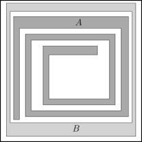
Figure 4.3: Illustration of two specific types of corridors: spirals (A) and rings (B)..

Lemma 48 (Corridor Packing Lemma, Adamaszek and Wiese [2015]).

There exists a corridor partition and a set $OPT_{corr}\subseteq OPT_{skew}$ such that:

1. there is a subset $OPT_{corr}^{cross}\subseteq OPT_{corr}$ with$|OPT_{corr}^{cross}|\leq O_{\varepsilon}(1)$ such that each item $i\in OPT_{corr}\setminus OPT_{corr}^{cross}$ is fully contained in some corridor,

2. $p(OPT_{corr})\geq(1-O(\varepsilon))p(OPT_{skew})$,

3. the number of corridors is $O_{\varepsilon,\varepsilon_{large}}(1)$ and each corridor has width at most $\varepsilon_{large}N$ and has at most $1/\varepsilon$ bends.

Since we are allowed to drop $O_{\varepsilon}(1)$ items from now on we ignore $OPT_{corr}^{cross}$. We next identify some structural properties of the corridors that are later exploited in our analysis. Observe that an open (resp. closed) corridor of the above type is the union of $k-1$ (resp. $k$) boxes, that we next call subcorridors (see also Figure 4.4). Each such box is a maximally large rectangle that is contained in the corridor. The subcorridor $S_{i}$ of an open (resp. closed) corridor of the above kind is the one containing edges $e_{i},e_{2k-i}$ (resp. $e_{i},e_{i^{\prime}}$) on its boundary. The length of $S_{i}$ is the length of the shortest such edge. We say that a subcorridor is long if its length is more than $N/2$, and short otherwise. The partition of subcorridors into short and long will be crucial in our analysis.

We call a subcorridor horizontal (resp. vertical) if the corresponding edges are so. Note that each rectangle in $OPT_{corr}$ is univocally associated with the only subcorridor that fully contains it: indeed, the longer side of a skewed rectangle is longer than the width of any corridor. Consider the sequence of consecutive subcorridors $S_{1},\ldots,S_{k^{\prime}}$ of an open or closed corridor. Consider two consecutive corridors $S_{i}$ and $S_{i^{\prime}}$, with $i^{\prime}=i+1$ in the case of an open corridor and $i^{\prime}=(i+1)\pmod{k^{\prime}}$ otherwise. First assume that $S_{i^{\prime}}$ is horizontal. We say that $S_{i^{\prime}}$ is to the right (resp. left) of $S_{i}$ if the right-most (left-most) boundary of $S_{i^{\prime}}$ is to the right (left) of the right-most (left-most) boundary of $S_{i}$. If instead $S_{i^{\prime}}$ is vertical, then $S_{i}$ must be horizontal and we say that $S_{i^{\prime}}$ is to the right (left) of $S_{i}$ if $S_{i}$ is to the left (right) of $S_{i^{\prime}}$. Similarly, if $S_{i^{\prime}}$ is vertical, we say that $S_{i^{\prime}}$ is above (below) $S_{i}$ if the top (bottom) boundary of $S_{i^{\prime}}$ is above (below) the top (bottom) boundary of $S_{i}$. If $S_{i^{\prime}}$ is horizontal, we say that it is above (below) $S_{i}$ if $S_{i}$ (which is vertical) is below (above) $S_{i^{\prime}}$. We say that the pair $(S_{i},S_{i^{\prime}})$ forms a clockwise bend if $S_{i}$ is horizontal and $S_{i^{\prime}}$ is to its bottom-right or top-left, and the complementary cases if $S_{i}$ is vertical. In all the other cases the pairs form a counter-clockwise bend. Consider a triple $(S_{i},S_{i^{\prime}},S_{i^{\prime\prime}})$ of consecutive subcorridors in the above sense. It forms a $U$-bend if $(S_{i},S_{i^{\prime}})$ and $(S_{i^{\prime}},S_{i^{\prime\prime}})$ are both clockwise or counterclockwise bends. Otherwise it forms a $Z$-bend. In both cases $S_{i^{\prime}}$ is the center of the bend, and $S_{i},S_{i^{\prime\prime}}$ its sides. An open corridor whose bends are all clockwise (resp. counter-clockwise) is a spiral. A closed corridor with $k=4$ is a ring. Note that in a ring all bends are clockwise or counter-clockwise, hence in some sense it is the closed analogue of a spiral. We remark that a corridor whose subcorridors are all long is a spiral or a ring. As we will see, spirals and rings play a crucial role in our analysis. In particular, we will exploit the following simple fact.

Lemma 49.

The following properties hold:

1. The two sides of a $Z$-bend cannot be long. In particular, an open corridor whose subcorridors are all long is a spiral.

2. A closed corridor contains at least $4$ distinct (possibly overlapping) $U$-bends.

Proof.

(1) By definition of long subcorridors and $Z$-bend, the $3$ subcorridors of the $Z$-bend would otherwise have total width or height larger than $N$. (2) Consider the left-most and right-most vertical subcorridors, and the top-most and bottom-most horizontal subcorridors. These $4$ subcorridors exist, are distinct, and are centers of a $U$-bend. ∎

4.3.3 Partitioning Corridors into Rectangular Boxes

We next describe a routine to partition the corridors into rectangular boxes such that each item is contained in one such box. We remark that to achieve this partitioning we sometimes have to sacrifice a large fraction of $OPT_{corr}$, hence we do not achieve a $1+\varepsilon$ approximation as in Adamaszek and Wiese [2013]. On the positive side, we generate only a constant (rather than polylogarithmic) number of boxes. This is crucial to obtain a polynomial time algorithm in the later steps.

Recall that each $i\in OPT_{corr}$ is univocally associated with the only subcorridor that fully contains it. We will say that we delete a sub-corridor, when we delete all rectangles univocally associated with the subcorridor. Note that in deletion of a sub-corridor we do not delete rectangles that are partially contained in that subcorridor but completely contained in a neighbor sub-corridor. Given a corridor, we sometimes delete some of its subcorridors, and consider the residual corridors (possibly more than one) given by the union of the remaining subcorridors. Note that removing any subcorridor from a closed corridor turns it into an open corridor. We implicitly assume that items associated with a deleted subcorridor are also removed (and consequently the corresponding area can be used to pack other items).

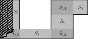
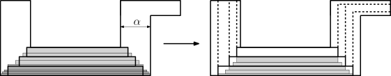
Figure 4.4: Left: The subcorridors $S_{1}$ and $S_{3}$ are vertical, $S_{2}$ and $S_{4}$ are horizontal. The subcorridor $S_{3}$ is on the top-right of $S_{2}$. The curve on the bottom left shows the boundary curve between $S_{1}$ and $S_{2}$. The pair $(S_{3},S_{4})$ forms a clockwise bend and the pair $(S_{2},S_{3})$ forms a counter-clockwise bend. The triple $(S_{1},S_{2},S_{3})$ forms a $U$-bend and the triple $(S_{2},S_{3},S_{4})$ forms a $Z$-bend. Right: Our operation that divides a corridor into $O_{\varepsilon}(1)$ boxes and $O_{\varepsilon}(1)$ shorter corridors. The dark gray items show thin items that are removed in this operation. The light gray items are fat items that are shifted to the box below their respective original box. The value $\alpha$ denotes the width of the depicted corridor.

Given two consecutive subcorridors $S_{i}$ and $S_{i^{\prime}}$, we define the boundary curve among them as follows (see also Figure 4.4). Suppose that $S_{i^{\prime}}$ is to the top-right of $S_{i}$, the other cases being symmetric. Let $S_{i,i^{\prime}}=S_{i}\cap S_{i^{\prime}}$ be the rectangular region shared by the two subcorridors. Then the boundary curve among them is any simple rectilinear polygon inside $S_{i,i^{\prime}}$ that decreases monotonically from its top-left corner to its bottom-right one and that does not cut any rectangle in these subcorridors. For a boundary horizontal (resp. vertical) subcorridor of an open corridor (i.e., a subcorridor containing $e_{0}$ or $e_{2k-1}$) we define a dummy boundary curve given by the vertical (resp. horizontal) side of the subcorridor that coincides with a (boundary) edge of the corridor.

Remark.

Each subcorridor has two boundary curves (including possibly dummy ones). Furthermore, all its items are fully contained in the region delimited by such curves plus the two edges of the corridor associated with the subcorridor (private region).

Given a corridor, we partition its area into a constant number of boxes as follows (see also Figure 4.4, and Adamaszek and Wiese [2013] for a more detailed description of an analogous construction). Let $S$ be one of its boundary subcorridors (if any), or the central subcorridor of a $U$-bend. Note that one such $S$ must exist (trivially for an open corridor, otherwise by Lemma 49.2). In the corridor partition, there might be several subcorridors fulfilling the latter condition. We will explain later in which order to process the subcorridors, here we explain only how to apply our routine to one subcorridor, which we call processing of subcorridor..

Suppose that $S$ is horizontal with height $b$, with the shorter horizontal associated edge being the top one. The other cases are symmetric. Let $\varepsilon_{box}>0$ be a sufficiently small constant to be defined later. If $S$ is the only subcorridor in the considered corridor, $S$ forms a box and all its items are marked as fat. Otherwise, we draw $1/\varepsilon_{box}$ horizontal lines that partition the private region of $S$ into subregions of height $\varepsilon_{box}b$. We mark as thin the items of the bottom-most (i.e., the widest) such subregion, and as killed the items of the subcorridor cut by these horizontal lines. All the remaining items of the subcorridor are marked as fat.

For each such subregion, we define an associated (horizontal) box as the largest axis-aligned box that is contained in the subregion. Given these boxes, we partition the rest of the corridor into $1/\varepsilon_{box}$ corridors as follows. Let $S^{\prime}$ be a corridor next to $S$, say to its top-right. Let $P$ be the set of corners of the boxes contained in the boundary curve between $S$ and $S^{\prime}$. We project $P$ vertically on the boundary curve of $S^{\prime}$ not shared with $S$, hence getting a set $P^{\prime}$ of $1/\varepsilon_{box}$ points. We iterate the process on the pair $(S^{\prime},P^{\prime})$. At the end of the process, we obtain a set of $1/\varepsilon_{box}$ boxes from the starting subcorridor $S$, plus a collection of $1/\varepsilon_{box}$ new (open) corridors each one having one less bend with respect to the original corridor. Later, we will also apply this process on the latter corridors. Each newly created corridor will have one bend less than the original corridor and thus this process eventually terminates. Note that, since initially there are $O_{\varepsilon,\varepsilon_{large}}(1)$ corridors each one with $O(1/\varepsilon)$ bends, the final number of boxes is $O_{\varepsilon,\varepsilon_{large},\varepsilon_{box}}(1)$. See Figure 4.4 for an illustration.

Remark.

Assume that we execute the above procedure on the subcorridors until there is no subcorridor left on which we can apply it. Then we obtain a partition of $OPT_{corr}$ into disjoint sets $OPT_{thin}$, $OPT_{fat}$, and $OPT_{kill}$ of thin, fat, and killed items, respectively. Note that each order to process the subcorridors leads to different such partition. We will define this order carefully in our analysis.

Remark.

By a simple shifting argument, there exists a packing of $OPT_{fat}$ into the boxes. Intuitively, in the above construction each subregion is fully contained in the box associated with the subregion immediately below (when no lower subregion exists, the corresponding items are thin).

We will from now on assume that the shifting of items as described in Remark Remark has been done.

The following lemma summarizes some of the properties of the boxes and of the associated partition of $OPT_{corr}$ (independently from the way ties are broken). Let $R_{hor}$ and $R_{ver}$ denote the set of horizontal and vertical input items, respectively.

Lemma 50.

The following properties hold:

1. $|OPT_{kill}|=O_{\varepsilon,\varepsilon_{large},\varepsilon_{box}}(1)$;

2. For any given constant $\varepsilon_{ring}>0$ there is a sufficiently small $\varepsilon_{box}>0$ such that the total height (resp. width) of items in $OPT_{thin}\cap R_{hor}$ (resp. $OPT_{thin}\cap R_{ver}$) is at most $\varepsilon_{ring}N$.

Proof.

(1) Each horizontal (resp. vertical) line in the construction can kill at most $1/\varepsilon_{large}$ items, since those items must be horizontal (resp. vertical). Hence we kill $O_{\varepsilon,\varepsilon_{large},\varepsilon_{box}}(1)$ items in total.

(2) The mentioned total height/width is at most $\varepsilon_{box}N$ times the number of subcorridors, which is $O_{\varepsilon,\varepsilon_{large}}(1)$. The claim follows for $\varepsilon_{box}$ small enough. ∎

4.3.4 Containers

Assume that we applied the routine described in Section 4.3.3 above until each corridor is partitioned into boxes. We explain how to partition each box into $O_{\varepsilon}(1)$ subboxes, to which we refer to as containers in the sequel. Hence, we apply the routine described below to each box.

Consider a box of size $a\times b$ coming from the above construction, and on the associated set $OPT_{box}$ of items from $OPT_{fat}$. We will show how to pack a set $OPT_{box}^{\prime}\subseteq OPT_{box}$ with $p(OPT_{box}^{\prime})\geq(1-\varepsilon)p(OPT_{box})$ into $O_{\varepsilon}(1)$ containers packed inside the box, such that both the containers and the packing of $OPT_{box}^{\prime}$ inside them satisfy some extra properties that are useful in the design of an efficient algorithm. This part is similar in spirit to prior work, though here we present a refined analysis that simplifies the algorithm (in particular, we can avoid LP rounding).

A container is a box labeled as horizontal, vertical, or area. A container packing of a set of items $I^{\prime}$ into a collection of non-overlapping containers has to satisfy the following properties:

• Items in a horizontal (resp. vertical) container are stacked one on top of the other (resp. one next to the other).

• Each $i\in I^{\prime}$ packed in an area container of size $a\times b$ must have $w_{i}\leq\varepsilon a$ and $h_{i}\leq\varepsilon b$.

Our main building block is the resource augmentation packing Lemma 14. Applying it to each box yields the following lemma.

Lemma 51 (Container Packing Lemma).

For a given constant $\varepsilon_{ra}>0$, there exists a set $OPT_{fat}^{cont}\subseteq OPT_{fat}$ such that there is a container packing for all apart from $O_{\varepsilon}(1)$ items in $OPT_{fat}^{cont}$ such that:

1. $p(OPT_{fat}^{cont})\geq(1-O(\varepsilon))p(OPT_{fat})$;

2. The number of containers is $O_{\varepsilon,\varepsilon_{large},\varepsilon_{box},\varepsilon_{ra}}(1)$ and their sizes belong to a set of cardinality $n^{O_{\varepsilon,\varepsilon_{large},\varepsilon_{box},\varepsilon_{ra}}(1)}$ that can be computed in polynomial time.

Proof.

Let us focus on a specific box of size $a\times b$ from the previous construction in Section 4.3.3, and on the items $OPT_{box}\subseteq OPT_{fat}$ inside it. If $|OPT_{box}|=O_{\varepsilon}(1)$ then we can simply create one container for each item and we are done. Otherwise, assume without loss of generality that this box (hence its items) is horizontal. We obtain a set $\overline{OPT_{box}}$ by removing from $OPT_{box}$ all items intersecting a proper horizontal strip of height $3\varepsilon b$. Clearly these items can be repacked in a box of size $a\times(1-3\varepsilon)b$. By a simple averaging argument, it is possible to choose the strip so that the items fully contained in it have total profit at most $O(\varepsilon)p(OPT_{box})$. Furthermore, there can be at most $O(1/\varepsilon_{large})$ items that partially overlap with the strip (since items are skewed). We drop these items and do not pack them.

At this point we can use the Resource Augmentation Lemma 14 to pack a large profit subset $OPT_{box}^{\prime}\subseteq\overline{OPT_{box}}$ into $O_{\varepsilon_{ra}}(1)$ containers that can be packed in a box of size $a\times(1-3\varepsilon)(1+\varepsilon_{ra})b\leq a\times(1-2\varepsilon)b$. We perform the above operation on each box of the previous construction and define $OPT_{fat}^{cont}$ to be the union of the respective sets $OPT_{box}^{\prime}$. The claim follows. ∎

4.3.5 A Profitable Structured Packing

We next prove our main structural lemma which yields that there exists a structured packing which is partitioned into $O_{\varepsilon}(1)$ containers and an L. We will refer to such a packing as an L&C packing (formally defined below). Note that in the previous section we did not specify in which order we partition the subcorridors into boxes. In this section, we give several such orders which will then result in different packings. The last such packing is special since we will modify it a bit to gain some space and then reinsert the thin items that were removed in the process of partitioning the corridors into containers. Afterwards, we will show that one of the resulting packings will yield an approximation ratio of $17/9+\varepsilon$.

A boundary ring of width $N^{\prime}$ is a ring having as external boundary the edges of the knapsack and as internal boundary the boundary of a square box of size $(N-N^{\prime})\times(N-N^{\prime})$ in the middle of the knapsack. A boundary $L$ of width $N^{\prime}$ is the region covered by two boxes of size $N^{\prime}\times N$ and $N\times N^{\prime}$ that are placed on the left and bottom boundaries of the knapsack.

An L&C packing is defined as follows. We are given two integer parameters $N^{\prime}\in[0,N/2]$ and $\ell\in(N/2,N]$. We define a boundary $L$ of width $N^{\prime}$, and a collection of non-overlapping containers contained in the space not occupied by the boundary $L$. The number of containers and their sizes are as in Lemma 51. We let $I_{\mathrm{long}}\subseteq I$ be the items whose longer side has length longer than $\ell$ (hence longer than $N/2$), and $I_{\mathrm{short}}=I\setminus I_{\mathrm{long}}$ be the remaining items. We can pack only items from $I_{\mathrm{long}}$ in the boundary $L$, and only items from $I_{\mathrm{short}}$ in the containers (satisfying the usual container packing constraints). See also Figure 4.1.

Remark.

In the analysis sometimes we will not need the boundary $L$. This case is captured by setting $N^{\prime}=0$ and $\ell=N$ (degenerate $L$ case).

Lemma 52.

Let $OPT_{L\&C}$ be the most profitable solution that is packed by an L&C packing. Then $p(OPT_{L\&C})\geq(\frac{9}{17}-O(\varepsilon))p(OPT)$.

In the remainder of this section we prove Lemma 52, assuming that we can drop $O_{\varepsilon}(1)$ items at no cost. Hence, formally we will prove that there is an L&C packing $I^{\prime}$ and a set of $O_{\varepsilon}(1)$ items $I_{\mathrm{drop}}$ such that $p(I^{\prime})+p(I_{\mathrm{drop}})\geq(\frac{9}{17}-O(\varepsilon))p(OPT)$. Subsequently, we will prove Lemma 52 in full generality (without dropping any items).

The proof of Lemma 52 involves some case analysis. Recall that we classify subcorridors into short and long, and horizontal and vertical. We further partition short subcorridors as follows: let $S_{1},\ldots,S_{k^{\prime}}$ be the subcorridors of a given corridor, and let $S_{1}^{s},\ldots,S_{k^{\prime\prime}}^{s}$ be the subsequence of short subcorridors (if any). Mark $S_{i}^{s}$ as even if $i$ is so, and odd otherwise. Note that corridors are subdivided into several other corridors during the box construction process (see the right side of Figure 4.4), and these new corridors might have fewer subcorridors than the initial corridor. However, the marking of the subcorridors (short, long, even, odd, horizontal, vertical) is inherited from the marking of the original subcorridor.

We will describe now 7 different ways to partition the subcorridors into boxes, for some of them we delete some of the subcorridors. Each of these different processing orders will give different sets $OPT_{thin},OPT_{kill}$ and $OPT_{fat}^{cont}$, and based on these, we will partition the items into three sets. We will then prove three different lower bounds on $p(OPT_{L\&C})$ with respect to the sizes of these three sets using averaging arguments about the seven cases.

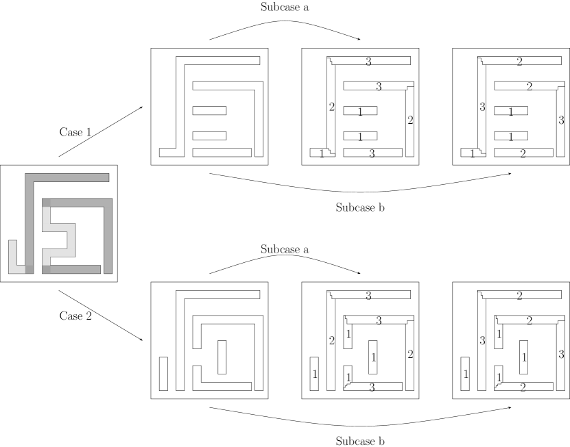
Figure 4.5: Figure for Case 1 and 2. The knapsack on the left contains two corridors, where short subcorridors are marked light gray and long subcorridors are marked dark gray. In case 1, we delete vertical short subcorridors and then consider two processing orders in subcases a and b. In case 2, we delete horizontal short subcorridors and again consider two processing orders in subcases a and b.

Cases 1a, 1b, 2a, 2b: Short horizontal/short vertical subcorridors.

We delete either all vertical short (case 1) or all horizontal short subcorridors (case 2). We first process all short subcorridors, then either all vertical (subcases a) or horizontal long ones (subcases b), and finally the remaining (horizontal or vertical, resp.) long ones. We can start by processing all short corridors. Indeed, any such corridor cannot be the center of a $Z$-bend by Lemma 49.1 since its two sides would be long, hence it must be boundary or the center of a $U$-bend. After processing short subcorridors, by the same argument the residual (long) subcorridors are the boundary or the center of a $U$-bend. So we can process the long subcorridors in any order. This gives in total four cases. See Figure 4.5 for deletion/processing of subcorridors for these cases.

Cases 3a, 3b: Even/odd short subcorridors.

We delete the odd (or even) short subcorridors and then process even (resp. odd) short subcorridors last. We exploit the fact that each residual corridor contains at most one short subcorridor. Then, if there is another (long) subcorridor, there is also one which is boundary (trivially for an open corridor) or the center of a $U$-bend (by Lemma 49, Property 2). Hence we can always process some long subcorridor leaving the unique short subcorridor as last one. This gives two cases.

Case 4: Fat only.

Do not delete any short subcorridor. Process subcorridors in any feasible order.

In each of the cases, we apply the procedure described in Section 4.3.4 to partition each box into $O_{\varepsilon}(1)$ containers. We next label items as follows. Consider the classification of items into $OPT_{fat}^{cont}$, $OPT_{thin}$, and $OPT_{kill}$ in each one of the $7$ cases above. Then:

• $OPT_{T}$ is the set of items which are in $OPT_{thin}$ in at least one case;

• $OPT_{K}$ is the set of items which are in $OPT_{kill}$ in at least one case;

• $OPT_{F}$ is the set of items which are in $OPT_{fat}^{cont}$ in all the cases.

Remark.

Consider the subcorridor of a given corridor that is processed last in one of the above cases. None of its items are assigned to $OPT_{thin}$ in that case and thus essentially all its items are packed in one of the constructed containers. In particular, for an item in set $OPT_{T}$, in some of the above cases it might be in such a subcorridor and thus marked fat and packed into a container.

Lemma 53.

One has:

$$p(OPT_{F}\cup OPT_{T})+p(OPT_{K})+p(OPT_{large})+p(OPT_{corr}^{cross})\geq(1-O(\varepsilon))p(OPT).$$

Proof.

Let us initialize $OPT_{F}=OPT_{fat}^{cont}$, $OPT_{T}=OPT_{thin}$, and $OPT_{K}=OPT_{kill}$ by considering one of the above cases. Next we consider the aforementioned cases, hence moving some items in $OPT_{F}$ to either $OPT_{T}$ or $OPT_{K}$. Note that initially $p(OPT_{F}\cup OPT_{T})+p(OPT_{kill})+p(OPT_{large})+p(OPT_{corr}^{cross})\geq(1-O(\varepsilon))p(OPT)$ by Lemma 48 and hence we keep this property.∎

Let $I_{\mathrm{lc}}$ and $I_{\mathrm{sc}}$ denote the items in long and short corridors, respectively. We also let $OPT_{LF}=I_{\mathrm{l}c}\cap OPT_{F}$, and define analogously $OPT_{SF}$, $OPT_{LT}$, and $OPT_{LF}$. The next three lemmas provide a lower bound on the case of a degenerate L.

Lemma 54.

$p(OPT_{L\&C})\geq p(OPT_{LF})+p(OPT_{SF}).$

Proof.

Follows immediately since we pack a superset of $OPT_{F}$ in case 4. ∎

Lemma 55.

$p(OPT_{L\&C})\geq p(OPT_{LF})+p(OPT_{LT})/2+p(OPT_{SF})/2.$

Proof.

Consider the sum of the profit of the packed items corresponding to the in total four subcases of cases 1 and 2. Each $i\in OPT_{LF}$ appears $4$ times in the sum (as items in $OPT_{F}$ are fat in all cases and all long subcorridors get processed), and each $i\in OPT_{LT}$ at least twice by Remark Remark: If a long subcorridor $\mathfrak{L}$ neighbors a short subcorridor, the short subcorridor is either deleted or processed first. Further, all neighboring long subcorridors are processed first in case 1a and 2a (if $\mathfrak{L}$ is horizontal, then its neighbors are vertical) or 1b and 2b (if $\mathfrak{L}$ is vertical and its neighbors are horizontal). Thus, $\mathfrak{L}$ is the last processed subcorridor in at least two cases. Additionally, each item $i\in OPT_{SF}$ also appears twice in the sum, as it gets deleted either in case 1 (if it is vertical) or in case 2 (if it is horizontal) and is fat otherwise.

The claim follows by an averaging argument. ∎

Lemma 56.

$p(OPT_{L\&C})\geq p(OPT_{LF})+p(OPT_{SF})/2+p(OPT_{ST})/2.$

Proof.

Consider the sum of the number of packed items corresponding to cases 3a and 3b. Each $i\in OPT_{LF}$ appears twice in the sum as it is fat and all long subcorridors get processed. Each $i\in OPT_{SF}\cup OPT_{ST}$ appears at least once in the sum by Remark Remark: An item $i\in OPT_{SF}$ is deleted in one of the two cases (depending on whether it is in an even or odd subcorridor) and otherwise fat. An item $i\in OPT_{ST}$ is also deleted in one of the two cases and otherwise its subcorridor is processed last. The claim follows by an averaging argument. ∎

There is one last (and slightly more involved) case to be considered, corresponding to a non-degenerate $L$.

Lemma 57.

$p(OPT_{L\&C})\geq\frac{3}{4}p(OPT_{LT})+p(OPT_{ST})+\frac{1-O(\varepsilon)}{2}p(OPT_{SF}).$

Proof.

Recall that $\varepsilon_{large}N$ is the maximum width of a corridor. We consider an execution of the algorithm with boundary $L$ width $N^{\prime}=\varepsilon_{ring}N$, and threshold length $\ell=(\frac{1}{2}+2\varepsilon_{large})N$. We remark that this length guarantees that items in $I_{\mathrm{long}}$ are not contained in short subcorridors.

By Lemma 45, we can pack a subset of $OPT_{T}\cap I_{\mathrm{long}}$ of profit at least $\frac{3}{4}p(OPT_{T}\cap I_{\mathrm{long}})$ in a boundary $L$ of width $\varepsilon_{ring}N$. By Lemma 50 the remaining items in $OPT_{T}$ can be packed in two containers of size $\ell\times\varepsilon_{ring}N$ and $\varepsilon_{ring}N\times\ell$ that we place on the two sides of the knapsack not occupied by the boundary $L$.

In the free area we can identify a square region $K^{\prime\prime}$ with side length $(1-\varepsilon)N$. We next show that there exists a feasible solution $OPT_{SF}^{\prime}\subseteq OPT_{SF}$ with $p(OPT_{SF}^{\prime})\geq(1-O(\varepsilon))p(OPT_{SF})/2$ that can be packed in a square of side length $(1-3\varepsilon)N$. We can then apply the Resource Augmentation Lemma 14 to pack $OPT_{SF}^{\prime\prime}\subseteq OPT_{SF}^{\prime}$ of cardinality $p(OPT_{SF}^{\prime\prime})\geq(1-O(\varepsilon))p(OPT_{SF}^{\prime})$ inside a central square region of side length $(1-3\varepsilon)(1+\varepsilon_{ra})N\leq(1-2\varepsilon)N$ using containers according to Lemma 51.

Consider the packing of $OPT_{SF}$ as in the optimum solution. Choose a random vertical (resp. horizontal) strip in the knapsack of width (resp. height) $3\varepsilon N$. Delete from $OPT_{SF}$ all the items intersecting the vertical and horizontal strips: clearly the remaining items $OPT_{SF}^{\prime}$ can be packed into a square of side length $(1-3\varepsilon)N$. Consider any $i\in OPT_{SF}$, and assume $i$ is horizontal (the vertical case being symmetric). Recall that it has height at most $\varepsilon_{small}N\leq\varepsilon N$ and width at most $\ell\leq 1/2+2\varepsilon$. Therefore $i$ intersects the horizontal strip with probability at most $5\varepsilon$ and the vertical strip with probability at most $1/2+8\varepsilon$. Thus by the union bound $i\in OPT_{SF}^{\prime}$ with probability at least $1/2-13\varepsilon$. The claim follows by linearity of expectation. ∎

Combining the above Lemmas 53, 54, 55, 56, and 57 we achieve the desired approximation factor, assuming that the (dropped) $O_{\varepsilon}(1)$ items in $OPT_{kill}\cup OPT_{large}\cup OPT_{corr}^{cross}$ have zero profit. The worst case is obtained, up to $1-O(\varepsilon)$ factors, for $p(OPT_{LT})=p(OPT_{SF})=p(OPT_{ST})$ and $p(OPT_{LF})=5p(OPT_{LT})/4$. This gives $p(OPT_{LT})=4/17\cdot p(OPT_{T}\cup OPT_{F})$ and a total profit of $9/17\cdot p(OPT_{T}\cup OPT_{F})$.

4.3.6 Adding small items

Note that up to now we ignored the small items $OPT_{small}$. In this section, we explain how to pack a large fraction of these items.

We described above how to pack a large enough fraction of $OPT_{skew}$ into containers. We next refine the mentioned analysis to bound the total area of such containers. It turns out that the residual area is sufficient to pack almost all the items of $OPT_{small}$ into a constant number of area containers (not overlapping with the previous containers) for $\varepsilon_{small}$ small enough.

To this aim we use the last of the properties given by the Resource Augmentation Lemma 14: in fact, the lemma guarantees that the total area of the containers is at most $a(I^{\prime})+\varepsilon_{ra}\,a\cdot b$, where $a\times b$ and $I^{\prime}$ are the size of the box and the initial set of items in the claim of Lemma 14, respectively.

Lemma 58.

In the packings due to Lemmas 54, 55, 56, and 57 the total area occupied by containers is at most $\min\{(1-2\varepsilon)N^{2},a(OPT_{corr})+\varepsilon_{ra}N^{2}\}$.

Proof.

Consider the first upper bound on the area. We have to distinguish between the containers considered in Lemma 57 and the remaining cases. In the first case, there is a region not occupied by the boundary $L$ nor by the containers of area at least $4\varepsilon N^{2}-4\varepsilon^{2}N^{2}-4\varepsilon_{ring}N^{2}\geq 2\varepsilon N^{2}$ for $\varepsilon_{ring}$ small enough, e.g., $\varepsilon_{ring}\leq\epsilon^{2}$ suffices. The claim follows. For the remaining cases, recall that in each horizontal box of size $a\times b$ we remove a horizontal strip of height $3\varepsilon b$, and then use the Resource Augmentation Packing Lemma to pack the residual items in a box of size $a\times b(1-3\varepsilon)(1+\varepsilon_{ra})\leq a\times b(1-2\varepsilon)$ for $\varepsilon_{ra}\leq\varepsilon$. Thus the total area of the containers is at most a fraction $1-2\varepsilon$ of the area of the original box. A symmetric argument applies to vertical boxes. Thus the total area of the containers is at most a fraction $1-2\varepsilon$ of the total area of the boxes, which in turn is at most $N^{2}$. This gives the first upper bound in the claim.

For the second upper bound, we just apply the area bound in Lemma 14 to get that the total area of the containers is at most $a(OPT_{corr})$ plus $\varepsilon_{ra}\,a\cdot b$ for each box of size $a\times b$. Summing the latter terms over the boxes one obtains at most $\varepsilon_{ra}N^{2}$. ∎

We are now ready to state a lemma that provides the desired packing of small items. By slightly adapting the analysis we can guarantee that the boundary $L$ that we use to prove the claimed approximation ratio has width at most $\varepsilon^{2}N$.

Lemma 59 (Small Items Packing Lemma).

Suppose we are given a packing of non small items of the above type into $k$ containers of total area $A$ and, possibly, a boundary $L$ of width at most $\varepsilon^{2}N$. Then for $\varepsilon_{small}$ small enough it is possible to define $O_{\varepsilon_{small}}(1)$ area containers of size $\frac{\varepsilon_{small}}{\varepsilon}N\times\frac{\varepsilon_{small}}{\varepsilon}N$ neither overlapping with the containers nor with the boundary $L$ (if any) such that it is possible to pack $OPT_{small}^{\prime}\subseteq OPT_{small}$ of profit $p(OPT_{small}^{\prime})\geq(1-O(\varepsilon))p(OPT_{small})$ inside these new area containers.

Proof.

Let us build a grid of width $\varepsilon^{\prime}N=\frac{\varepsilon_{small}}{\varepsilon}\cdot N$ inside the knapsack. We delete any cell of the grid that overlaps with a container or with the boundary $L$, and call the remaining cells free. The new area containers are the free cells.

The total area of the deleted grid cells is, for $\varepsilon_{small}$ and $\varepsilon_{ra}$ small enough, at most

$$(\varepsilon^{2}N^{2}+A)+\frac{2N+4Nk}{\varepsilon^{\prime}N}\cdot(\varepsilon^{\prime}N)^{2} \leq A+2\varepsilon^{2}N^{2}$$

$$\overset{Lem.\ref{lem:areaContainer}}{\leq}\min\{(1-\varepsilon)N^{2},a(OPT_{corr})+3\varepsilon^{2}N^{2}\}$$

For the sake of simplicity, suppose that any empty space in the optimal packing of $OPT_{corr}\cup OPT_{small}$ is filled in with dummy small items of profit $0$, so that $a(OPT_{corr}\cup OPT_{small})=N^{2}$. We observe that the area of the free cells is at least $(1-O(\varepsilon))a(OPT_{small})$: Either, $a(OPT_{small})\geq\varepsilon N^{2}$ and then the area of the free cells is at least $a(OPT_{small})-3\varepsilon^{2}N^{2}\geq(1-3\varepsilon)a(OPT_{small})$; otherwise, we have that the area of the free cells is at least $\varepsilon N^{2}>a(OPT_{small})$. Therefore we can select a subset of small items $OPT_{small}^{\prime}\subseteq OPT_{small}$, with $p(OPT_{small}^{\prime})\geq(1-O(\varepsilon))p(OPT_{small})$ and area $a(OPT_{small})\leq(1-O(\varepsilon))a(OPT_{small})$ that can be fully packed into free cells using classical Next Fit Decreasing Height algorithm (NFDH) according to Lemma 1 described later. The key argument for this is that each free cell is by a factor $1/\varepsilon$ larger in each dimension than each small item. ∎

Thus, we have proven now that if the items in $OPT_{kill}\cup OPT_{large}\cup OPT_{corr}^{cross}$ had zero profit, then there is an L&C-packing for the skewed and small items with a profit of at least $9/17\cdot p(OPT_{corr})+(1-O(\epsilon))(OPT_{small})\geq(9/17-O(\epsilon))p(OPT)$.

4.3.7 Shifting argumentation

We remove now the assumption that we can drop $O_{\varepsilon}(1)$ items from $OPT$. We will add a couple of shifting steps to the argumentation above to prove Lemma 52 without that assumption.

It is no longer true that we can neglect the large rectangles $OPT_{large}$ since they might contribute a large amount towards the objective, even though their total number is guaranteed to be small. Also, in the process of constructing the boxes, we killed up to $O_{\varepsilon}(1)$ rectangles (the rectangles in $OPT_{kill}$). Similarly, we can no longer drop the constantly many items in $OPT_{corr}^{cross}$. Therefore, we apply some careful shifting arguments in order to ensure that we can still use a similar construction as above, while losing only a factor $1+O(\varepsilon)$ due to some items that we will discard.

The general idea is as follows: For $t=0,\ldots,k$ (we will later argue that $k<1/\varepsilon$), we define disjoint sets $K(t)$ recursively, each containing at most $O_{\varepsilon}(1)$ items. Each set $\mathcal{K}(t)=\bigcup_{j=0}^{t}K(j)$ is used to define a grid $G(t)$ in the knapsack. Based on an item classification that depends on this grid, we identify a set of skewed items and create a corridor partition with respect to these skewed items as described in Lemma 48. We then create a partition of the knapsack into corridors and a constant (depending on $\varepsilon$) number of containers (see Section 4.3.7). Next, we decompose the corridors into boxes (Section 4.3.7) and these boxes into containers (section 4.3.7) similarly as we did in Sections 4.3.3 and 4.3.4 (but with some notable changes as we did not delete small items from the knapsack and thus need to handle those as well). In the last step, we add small items to the packing (Section 4.3.7). During this whole process, we define the set $K(i+1)$ of items that are somehow “in our way” during the decomposition process (e.g., items that are not fully contained in some corridor of the corridor partition), but which we cannot delete directly as they might have large profit. These items are similar to the killed items in the previous argumentation. However, using a shifting argument we can simply show that after at most $k<1/\varepsilon$ steps of this process, we encounter a set $K(k)$ of low total profit, that we can remove, at which point we can apply almost the same argumentation as in Lemmas 54, 55, and 56 to obtain lower bounds on the profit of an optimal L&C packing (Section 4.3.7).

We initiate this iterative process as follows: Denote by $K(0)$ a set containing all items that are killed in at least one of the cases arising in Section 4.3.5 (the set $OPT_{K}$ in that Section) and additionally the large items $OPT_{large}$ and the $O_{\varepsilon}(1)$ items in $OPT_{corr}^{cross}$ (in fact $OPT_{large}\subseteq OPT_{corr}^{cross}$). Note that $|K(0)|\leq O_{\varepsilon}(1)$. If $p(K(0))\leq\varepsilon\cdot p(OPT)$ then we can simply remove these rectangles (losing only a factor of $1+\varepsilon$) and then apply the remaining argumentation exactly as above and we are done. Therefore, from now on suppose that $p(K(0))>\varepsilon\cdot p(OPT)$.

Definition of grid and corridor partition

Assume we are in round $t$ of this process, i.e., we defined $K(t)$ in the previous step (unless $t=0$, then $K(t)$ is defined as specified above) and assume that $p(K(t))>\varepsilon OPT$ (otherwise, see Section 4.3.7). We are now going to define the non-uniform grid $G(t)$ and the induced partition of the knapsack into a collection of cells $\mathcal{C}_{t}$. The $x$-coordinates ($y$-coordinates) of the grid cells are the $x$-coordinates ($y$-coordinates, respectively) of the items in $\mathcal{K}(t)$. This yields a partition of the knapsack into $O_{\varepsilon}(1)$ rectangular cells, such that each item of $\mathcal{K}(t)$ covers one or multiple cells. Note that an item might intersect many cells.

Similarly as above, we define constants $1\geq\varepsilon_{large}\geq\varepsilon_{small}\geq\Omega_{\varepsilon}(1)$ and apply a shifting step such that we can assume that for each item $i\in OPT$ touching some cell $C$ we have that $w(i\cap C)\in(0,\varepsilon_{small}w(C)]\cup(\varepsilon_{large}w(C),w(C)]$ and $h(i\cap C)\in(0,\varepsilon_{small}h(C)]\cup(\varepsilon_{large}h(C),h(C)]$, where $h(C)$ and $w(C)$ denote the height and the width of the cell $C$ and $w(i\cap C)$ and $h(i\cap C)$ denote the height and the width of the intersection of the rectangle $i$ with the cell $C$, respectively. For a cell $C$ denote by $OPT(C)$ the set of rectangles that intersect $C$ in $OPT$. We obtain a partition of $OPT(C)$ into $OPT_{small}(C)$, $OPT_{large}(C)$, $OPT_{hor}(C)$, and $OPT_{ver}(C)$:

• $OPT_{small}(C)$ contains all items $i\in OPT(C)$ with $h(i\cap C)\leq\varepsilon_{small}h(C)$ and $w(i\cap C)\leq\varepsilon_{small}w(C)$,

• $OPT_{large}(C)$ contains all items $i\in OPT(C)$ with $h(i\cap C)>\varepsilon_{large}h(C)$ and $w(i\cap C)>\varepsilon_{large}w(C)$,

• $OPT_{hor}(C)$ contains all items $i\in OPT(C)$ with $h(i\cap C)\leq\varepsilon_{small}h(C)$ and $w(i\cap C)>\varepsilon_{large}w(C)$, and

• $OPT_{ver}(C)$ contains all items $i\in OPT(C)$ with $h(i\cap C)>\varepsilon_{large}h(C)$ and $w(i\cap C)\leq\varepsilon_{small}w(C)$.

We call a rectangle $i$ intermediate if there is a cell $C$ such that $w(i\cap C)\in(\varepsilon_{small}w(C),\varepsilon_{large}w(C)]$ or $h(i\cap C)\in(\varepsilon_{small}w(C),\varepsilon_{large}w(C)]$. Note that a rectangle $i$ is intermediate if and only if the last condition is satisfied for one of the at most four cells that contain a corner of $i$.

Lemma 60.

For any constant $\varepsilon>0$ and positive increasing function $f(\cdot)$, $f(x)>x$, there exist constant values $\varepsilon_{large},\varepsilon_{small}$, with $\varepsilon\geq\varepsilon_{large}\geq f(\varepsilon_{small})\geq\Omega_{\varepsilon}(1)$ and $\varepsilon_{small}\in\Omega_{\varepsilon}(1)$ such that the total profit of intermediate rectangles is bounded by $\varepsilon p(OPT)$.

For each cell $C$ that is not entirely covered by some item in $K(t)$ we add all rectangles in $OPT_{large}(C)$ that are not contained in $\mathcal{K}(t)$ to $K(t+1)$. Note that here, in contrast to before, we do not remove small items from the packing but keep them.

Based on the items $OPT_{skew}(\mathcal{C}_{t}):=\cup_{C\in\mathcal{C}_{t}}OPT_{hor}(C)\cup OPT_{ver}(C)$ we create a corridor decomposition and consequently a box decomposition of the knapsack. To make this decomposition clearer, we assume that we first stretch the non-uniform grid into a uniform $[0,1]\times[0,1]$ grid. After this operation, for each cell $C$ and for each element of $OPT_{hor}(C)\cup OPT_{ver}(C)$ we know that its height or width is at least $\varepsilon_{large}\cdot\frac{1}{1+2|\mathcal{K}(t)|}$. We apply Lemma 48 on the set $OPT_{skew}(\mathcal{C}_{t})$ which yields a decomposition of the $[0,1]\times[0,1]$ square into at most $O_{\varepsilon,\varepsilon_{large},\mathcal{K}(t)}(1)=O_{\varepsilon,\varepsilon_{large}}(1)$ corridors. The decomposition for the stretched $[0,1]\times[0,1]$ square corresponds to the decomposition for the original knapsack, with the same items being intersected. Since we can assume that all items of $OPT$ are placed within the knapsack so that they have integer coordinates, we can assume that the corridors of the decomposition also have integer coordinates. We can do that, because shifting the edges of the decomposition to the closest integral coordinate will not make the decomposition worse, i.e., no new items of $OPT$ will be intersected.

We add all rectangles in $OPT_{skew}(\mathcal{C}_{t})$ that are not contained in a corridor (at most $O_{\varepsilon}(1)$ many) and that are not contained in $\mathcal{K}(t)$ to $K(t+1)$. The corridor partition has the following useful property: we started with a fixed (optimal) solution $OPT$ for the overall problem with a fixed placement of the items in this solution. Then we considered the items in $OPT_{skew}(\mathcal{C}_{t})$ and obtained the sets $OPT_{corr}\subseteq OPT_{skew}(\mathcal{C}_{t})$ and $OPT_{corr}^{cross}\subseteq OPT_{corr}$. With the mentioned fixed placement, apart from the $O_{\varepsilon}(1)$ items in $OPT_{corr}^{cross}$, each item in $OPT_{corr}$ is contained in one corridor. In particular, the items in $OPT_{corr}$ do not overlap the items in $\mathcal{K}(t)$. We construct now a partition of the knapsack into $O_{\varepsilon}(1)$ corridors and $O_{\varepsilon}(1)$ containers where each container contains exactly one item from $\mathcal{K}(t)$. The main obstacle is that there can be an item $i\in\mathcal{K}(t)$ that overlaps a corridor (see Figure 4.6). We solve this problem by applying the following lemma on each such corridor.

Lemma 61.

Let $S$ be an open corridor with $b(S)$ bends. Let $I^{\prime}\subseteq OPT$ be a collection of items which intersect the boundary of $S$ with $I^{\prime}\cap OPT_{skew}(\mathcal{C}_{t})=\emptyset$. Then there is a collection of $|I^{\prime}|\cdot b(S)$ line segments $\mathcal{L}$ within $S$ which partition $S$ into corridors with at most $b(S)$ bends each such that no item from $I^{\prime}$ is intersected by $\mathcal{L}$ and there are at most $O_{\varepsilon}(|I^{\prime}|\cdot b(S))$ items of $OPT_{skew}(\mathcal{C}_{t})$ intersected by line segments in $\mathcal{L}$.

Proof.

Let $i\in I^{\prime}$ and assume without loss of generality that $i$ lies within a horizontal subcorridor $S_{i}$ of the corridor $S$. If the top or bottom edge $e$ of $i$ lies within $S_{i}$, we define a horizontal line segment $\ell$ which contains the edge $e$ and which is maximally long so that it does not intersect the interior of any item in $I^{\prime}$, and such that it does not cross the boundary curve between $S_{i}$ and an adjacent subcorridor, or an edge of the boundary of $S$ (we can assume without loss of generality that $e$ does not intersect the boundary curve between $S_{i}$ and some adjacent subcorridor). We say that $\ell$ crosses a boundary curve $c$ (or an edge $e$ of the boundary of $S$) if $c\setminus\ell$ (or $e\setminus\ell$) has two connected components.

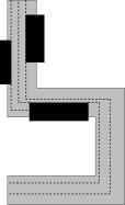
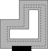
Figure 4.6: Circumventing the items in $I^{\prime}$, shown in black. The connected components between the dashed lines show the resulting new corridors.

We now “extend” each end-point of $\ell$ which does not lie at the boundary of some other item of $I^{\prime}$ or at the boundary of $S$, we call such an end point a loose end. For each loose end $x$ of $\ell$ lying on the boundary curve $c_{ij}$ partitioning the subcorridors $S_{i}$ and $S_{j}$, we introduce a new line $\ell^{\prime}$ perpendicular to $\ell$, starting at $x$ and crossing the subcorridor $S_{j}$ such that the end point of $\ell^{\prime}$ is maximally far away from $x$ subject to the constraint that $\ell^{\prime}$ does not cross an item in $I^{\prime}$, another boundary curve inside $S$, or the boundary of $S$. We continue iteratively. Since the corridor has $b(S)$ bends, after at most $b(S)$ iterations this operation will finish. We repeat the above operation for every item $i\in I^{\prime}$, and we denote by $\mathcal{L}$ the resulting set of line segments, see Figure 4.6 for a sketch. Notice that $|\mathcal{L}|=b(S)\cdot|I^{\prime}|$. By construction, if an item $i\in OPT_{skew}(\mathcal{C}_{t})$ is intersected by a line in $\mathcal{L}$ then it is intersected parallel to its longer edge. Thus, each line segment in $\mathcal{L}$ can intersect at most $O_{\varepsilon}(1)$ items of $OPT_{skew}(\mathcal{C}_{t})$. Thus, in total there are at most $O_{\varepsilon,\varepsilon_{large}}(|I^{\prime}|\cdot b(S))$ items of $OPT_{skew}(\mathcal{C}_{t})$ intersected by line segments in $\mathcal{L}$. ∎

We apply Lemma 61 to each open corridor that intersects an item in $\mathcal{K}(t)$. We add all items of $R_{skew}(\mathcal{C}_{t})$ that are intersected by line segments in $\mathcal{L}$ to $K(t+1)$. This adds $O_{\varepsilon}(1)$ items in total to $K(t+1)$ since $|\mathcal{K}(t)|\in O_{\varepsilon}(1)$ and $b(S)\leq 1/\varepsilon$ for each corridor $S$. For closed corridors we prove the following lemma.

Lemma 62.

Let $S$ be a closed corridor with $b(S)$ bends. Let $OPT_{skew}(S)$ denote the items in $OPT_{skew}(\mathcal{C}_{t})$ that are contained in $S$. Let $I^{\prime}\subseteq OPT$ be a collection of items which intersect the boundary of $S$ with $I^{\prime}\cap OPT_{skew}(\mathcal{C}_{t})=\emptyset$. Then there is a collection of $O_{\varepsilon}(|I^{\prime}|^{2}/\varepsilon)$ line segments $\mathcal{L}$ within $S$ which partition $S$ into a collection of closed corridors with at most $1/\varepsilon$ bends each and possibly an open corridor with $b(S)$ bends such that no item from $I^{\prime}$ is intersected by $\mathcal{L}$ and there is a set of items $OPT_{skew}^{\prime}(S)\subseteq OPT_{skew}(S)$ with $|OPT_{skew}^{\prime}(S)|\leq O_{\varepsilon}(|I^{\prime}|^{2})$ such that the items in $OPT_{skew}(S)\setminus OPT_{skew}^{\prime}(S)$ intersected by line segments in $\mathcal{L}$ have a total profit of at most $O(\varepsilon)\cdot p(OPT_{skew}(\mathcal{C}_{t}))$.

Proof.

Similarly as for the case of open corridors, we take each item $i\in I^{\prime}$ whose edge $e$ is contained in $S$, and we create a path containing $e$ that partitions $S$. Here the situation is a bit more complicated, as our newly created paths could extend over more than $\frac{1}{\varepsilon}$ bends inside $S$. In this case we will have to do some shortcutting, i.e., some items contained in $S$ will be crossed parallel to their shorter edge and we cannot guarantee that their total number will be small. However, we will ensure that the total weight of such items is small. We proceed as follows (see Figure 4.6 for a sketch).

Consider any item $i\in I^{\prime}$ and assume without loss of generality that $i$ intersects a horizontal subcorridor $S_{i}$ of the closed corridor $S$. Let $e$ be the edge of $i$ within $S_{i}$. For each endpoint of $e$ we create a path $p$ as for the case of closed corridors. If after at most $b(S)\leq 1/\varepsilon$ bends the path hits an item of $I^{\prime}$ (possibly the same item $i$), the boundary of $S$ or another path created earlier, we stop the construction of the path. Otherwise, if $p$ is the first path inside of $S$ that did not finish after at most $b(S)$ bends, we proceed with the construction of the path, only now at each bend we check the total weight of the items of $OPT_{skew}(S)$ that would be crossed parallel to their shorter edge, if, instead of bending, the path would continue at the bend to hit itself. From the construction of the boundary curves in the intersection of two subcorridors we know that for two bends of the constructed path, the sets of items that would be crossed at these bends of the path are pairwise disjoint. Thus, after $O(|I^{\prime}|/\varepsilon)$ bends we encounter a collection of items $OPT_{skew}^{\prime\prime}(S)\subseteq OPT_{skew}(S)$ such that $p(OPT_{skew}^{\prime\prime}(S))\leq\frac{\varepsilon}{|I^{\prime}|}p(OPT_{skew}(S))$, and we end the path $p$ by crossing the items of $OPT_{skew}^{\prime\prime}(S)$. This operation creates an open corridor with up to $O(|I^{\prime}|/\varepsilon)$ bends. We divide it into up to $O(|I^{\prime}|)$ corridors with up to $1/\varepsilon$ bends each. Via a shifting argument we can argue that this loses at most a factor of $1+\varepsilon$ in the profit due to these items. When we perform this operation for each item $i\in I^{\prime}$ the total weight of items intersected parallel to their shorter edge (i.e., due to the above shortcutting) is bounded by $|I^{\prime}|\cdot\frac{\varepsilon}{|I^{\prime}|}p(OPT_{skew}(S))=\varepsilon\cdot p(OPT_{skew}(S))$. This way, we introduce at most $O(|I^{\prime}|^{2}/\varepsilon)$ line segments. Denote them by $\mathcal{L}$. They intersect at most $O_{\varepsilon}(|I^{\prime}|^{2})$ items parallel to their respective longer edge, denote them by $OPT_{skew}^{\prime}(S)$. Thus, the set $\mathcal{L}$ satisfies the claim of the lemma. ∎

Similarly as for Lemma 61 we apply Lemma 62 to each closed corridor. We add all items in the respective set $OPT_{skew}^{\prime}(S)$ to the set $K(t+1)$ which yields $O_{\varepsilon}(1)$ many items. The items in $OPT_{skew}(S)\backslash OPT_{skew}^{\prime}(S)$ are removed from the instance, as their total profit is small.

Partitioning corridors into boxes

Then we partition the resulting corridors into boxes according to the different cases described in Section 4.3.5. There is one difference to the argumentation above: we define that the set $OPT_{fat}$ contains not only skewed items contained in the respective subregions of a subcorridor, but all items contained in such a subregion. In particular, this includes items that might have been considered as small items above. Thus, when we move items from one subregion to the box associated to the subregion below (see Remark Remark) then we move every item that is contained in that subregion. If an item is killed in one of the orderings of the subcorridors to apply the procedure from Section 4.3.3 then we add it to $K(t+1)$. Note that $|K(t+1)|\in O_{\varepsilon,\varepsilon_{large},\varepsilon_{box}}(1)$ and $\mathcal{K}(t)\cap K(t+1)=\emptyset$. Also note here that we ignore for the moment small items that cross the boundary curves of the subcorridors; they will be taken care of in Section 4.3.7.

Partitioning boxes into containers

Then we subdivide the boxes into containers. We apply Lemma 51 to each box with a slight modification. Assume that we apply it to a box of size $a\times b$ containing a set of items $I_{box}$. Like above we first remove the items in a thin strip of width $3\varepsilon b$ such that via a shifting argument the items (fully!) contained in this strip have a small profit of $O(\varepsilon)p(I_{box})$. However, in contrast to the setting above the set $I_{box}$ contains not only skewed items but also small items. We call an item $i$ small if there is no cell $C$ such that $i\in OPT_{large}(C)\cup OPT_{hor}(C)\cup OPT_{ver}(C)$ and denote by $OPT_{small}(\mathcal{C}_{t})$ the set of small items. When we choose the strip to be removed we ensure that the profit of the removed skewed and small items is small. There are $O_{\varepsilon}(1)$ skewed items that partially (but not completely) overlap the strip whose items we remove. We add those $O_{\varepsilon}(1)$ items to $K(t+1)$. Small items that partially overlap the strip are taken care of later in Section 4.3.7, we ignore them for the moment. Then we apply Lemma 14. In contrast to the setting above, we do not only apply it to the skewed items but apply it also to small items that are contained in the box. Denote by $OPT_{small}^{\prime}(\mathcal{C}_{t})$ the set of small items that are contained in some box of the box partition.

Thus, we obtain an L&C packing for the items in $\mathcal{K}(t)$, for a set of items $OPT_{skew}^{\prime}(\mathcal{C}_{t})\subseteq OPT_{skew}(\mathcal{C}_{t})$, and for a set of items $OPT_{small}^{\prime\prime}(\mathcal{C}_{t})\subseteq OPT_{small}^{\prime}(\mathcal{C}_{t})$ with total profit at least $(1-O(\varepsilon))p(OPT_{skew}(\mathcal{C}_{t})\cup OPT_{small}^{\prime}(\mathcal{C}_{t}))$.

Handling small items

So far we ignored the small items in $OPT_{small}^{\prime\prime}(\mathcal{C}_{t}):=OPT_{small}(\mathcal{C}_{t})\setminus OPT_{small}^{\prime}(\mathcal{C}_{t})$. This set consists of small items that in the original packing intersect a line segment of the corridor partition, the boundary of a box, or a boundary curve within a corridor. We describe now how to add them into the empty space of the so far computed packing. First, we assign each item in $OPT_{small}^{\prime\prime}(\mathcal{C}_{t})$ to a grid cell. We assign each small item $i\in OPT_{small}^{\prime\prime}(\mathcal{C}_{t})$ to the cell $C$ such that in the original packing $i$ intersects with $C$ and the area of $i\cap C$ is not smaller than $i\cap C^{\prime}$ for any cell $C^{\prime}$ ($i\cap C^{\prime}$ denotes the part of $i$ intersecting $C^{\prime}$ in the original packing for any grid cell $C^{\prime}$).

Consider a grid cell $C$ and let $OPT_{small}^{\prime\prime}(C)$ denote the small items in $OPT_{small}^{\prime\prime}(\mathcal{C}_{t})$ assigned to $C$. Intuitively, we want to pack them into the empty space in the cell $C$ that is not used by any of the containers, similarly as above. We first prove an analog of Lemma 58 of the setting above.

Lemma 63.

Let $C$ be a cell. The total area of $C$ occupied by containers is at most $(1-2\varepsilon)a(C)$.

Proof.

In our construction of the boxes we moved some of the items (within a corridor). In particular, it can happen that we moved some items into $C$ that were originally in some other grid cell $C^{\prime}$. This reduces the empty space in $C$ for the items in $OPT_{small}^{\prime\prime}(C)$. Assume that there is a horizontal subcorridor $H$ intersecting $C$ such that some items or parts of items within $H$ were moved into $C$ that were not in $C$ before. Then such items were moved vertically and the corridor containing $H$ must intersect the upper or lower boundary of $C$. The part of this subcorridor lying within $C$ has a height of at most $\varepsilon_{large}\cdot h(C)$. Thus, the total area of $C$ lost in this way is bounded by $O(\varepsilon_{large}a(C))$ which includes analogous vertical subcorridors.

Like in Lemma 58 we argue that in each horizontal box of size $a\times b$ we remove a horizontal strip of height $3\varepsilon b$ and then the created containers lie in a box of height $(1-3\varepsilon)(1+\varepsilon_{ra})b$. In particular, if the box does not intersect the top or bottom edge of $C$ then within $C$ its containers use only a box of dimension $a^{\prime}\times(1-3\varepsilon)(1+\varepsilon_{ra})b$ where $a^{\prime}$ denotes the width of the box within $C$, i.e., the width of the intersection of the box with $C$. If the box intersects the top or bottom edge of $C$ then we cannot guarantee that the free space lies within $C$. However, the total area of such boxes is bounded by $O(\varepsilon_{large}a(C))$. We can apply a symmetric argument to vertical boxes. Then, the total area of $C$ used by containers is at most $(1-3\varepsilon)(1+\varepsilon_{ra})a(C)+O(\varepsilon_{large}a(C))\leq(1-2\varepsilon)a(C)$. This gives the claim of the lemma. ∎

Next, we argue that the items in $OPT_{small}^{\prime\prime}(C)$ have very small total area. Recall that they are the items intersecting $C$ that are not contained in a box. The total number of boxes and boundary curves intersecting $C$ is $O_{\varepsilon,\varepsilon_{large}}(1)$ and in particular, this quantity does not depend on $\varepsilon_{small}$. Hence, by choosing $\varepsilon_{small}$ sufficiently small, we can ensure that $a(OPT_{small}^{\prime\prime}(C))\leq\varepsilon a(C)$. Then, similarly as in Lemma 59 we can argue that if $\varepsilon_{small}$ is small enough then we can pack the items in $OPT_{small}^{\prime\prime}(C)$ using NFDH into the empty space within $C$.

L&C packings

We iterate the above construction, obtaining pairwise disjoint sets $K(1),K(2),...$ until we find a set $K(k)$ such that $p(K(k))\leq\varepsilon\cdot OPT$. Since the sets $K(0),K(1),...$ are pairwise disjoint there must be such a value $k$ with $k\leq 1/\varepsilon$. Thus, $|\mathcal{K}(k-1)|\leq O_{\varepsilon}(1)$. We build the grid given by the $x$- and $y$-coordinates of $\mathcal{K}(k-1)$, giving a set of cells $\mathcal{C}_{k}$. As described above we define the corridor partition, the partition of the corridors into boxes (with the different orders to process the subcorridors as described in Section 4.3.3) and finally into containers. Denote by $OPT_{small}(\mathcal{C}_{k})$ the resulting set of small items.

We consider the candidate packings based on the grid $\mathcal{C}_{k}$. For each of the six candidate packings with a degenerate $L$ we can pack almost all small items of the original packing. We define $I_{\mathrm{lc}}$ and $I_{\mathrm{sc}}$ the sets of items in long and short subcorridors in the initial corridor partition, respectively. Exactly as in the cardinality case, a subcorridor is long if it is longer than $N/2$ and short otherwise. As before we divide the items into fat and thin items and define the sets $OPT_{SF}$, $OPT_{LT}$, and $OPT_{ST}$ accordingly. Moreover, we define the set $OPT_{LF}$ to contain all items in $I_{\mathrm{lc}}$ that are fat in all candidate packings plus the items in $\mathcal{K}(k-1)$.

Thus, we obtain the respective claims of Lemmas 54, 55, and 56 in the weighted setting. For the following lemma let $OPT_{small}:=OPT_{small}(\mathcal{C}_{k})$.

Lemma 64.

Let $OPT_{L\&C}$ the most profitable solution that is packed by an L&C packing.

1. $p(OPT_{L\&C})\geq(1-O(\varepsilon))(p(OPT_{LF})+p(OPT_{SF})+p(OPT_{small}))$

2. $p(OPT_{L\&C})\geq(1-O(\varepsilon))(p(OPT_{LF})+p(OPT_{SF})/2+p(OPT_{LT})/2+p(OPT_{small}))$

3. $p(OPT_{L\&C})\geq(1-O(\varepsilon))(p(OPT_{LF})+p(OPT_{SF})/2+p(OPT_{ST})/2+p(OPT_{small})).$

For the candidate packing for the non-degenerate-$L$ case (Lemma 57 in Section 4.3.5) we first add the small items as described above. Then we remove the items in $\mathcal{K}(k-1)$. Then, like above, with a random shift we delete items touching a horizontal and a vertical strip of width $3\varepsilon N$. Like before, each item $i$ is still contained in the resulting solution with probability $1/2-15\varepsilon$ (note that we cannot make such a claim for the items in $\mathcal{K}(k-1)$). For each small item we can even argue that it still contained in the resulting solution with probability $1-O(\varepsilon)$ (since it is that small in both dimensions). We proceed with the construction of the boundary $L$ and the assignment of the items into it like in the unweighted case.

Lemma 65.

For the solution $OPT_{L\&C}$ we have that $p(OPT_{L\&C})\geq(1-O(\varepsilon))(\frac{3}{4}p(OPT_{LT})+p(OPT_{ST})+\frac{1-O(\varepsilon)}{2}p(OPT_{SF})+p(OPT_{small}))$.

When we combine Lemmas 64 and 65 we conclude that $p(OPT_{L\&C})\geq(17/9+O(\varepsilon))p(OPT)$. Similarly as before, the worst case is obtained, up to $1-O(\varepsilon)$ factors, when we have that $p(OPT_{LT})=p(OPT_{SF})=p(OPT_{ST})$, $p(OPT_{LF})=5p(OPT_{LT})/4$, and $p(OPT_{small})=0$. This completes the proof of Lemma 52.

4.3.8 Main algorithm

In this Section we present our main algorithm for the weighted case of 2DGK. It is in fact an approximation scheme for L&C packings. Its approximation factor therefore follows immediately from Lemma 52.

Given $\epsilon>0$, we first guess the quantities $\varepsilon_{large},\varepsilon_{small}$, the proof of Lemma 47 reveals that there are only $2/\epsilon+1$ values we need to consider. We choose $\varepsilon_{ring}:=\epsilon^{2}$ and subsequently define $\varepsilon_{box}$ according to Lemma 50. Our algorithm combines two basic packing procedures. The first one is PTAS to pack items into a constant number of containers given by Theorem 12.

The second packing procedure is the PTAS for the L-packing problem, see Theorem 34.

To use these packing procedures, we first guess whether the optimal L&C-packing due to Lemma 52 uses a non-degenerate boundary L. If yes, we guess a parameter $\ell$ which denotes the minimum height of the vertical items in the boundary $L$ and the minimum width of the horizontal items in the boundary $L$. For $\ell$ we allow all heights and widths of the input items that are larger than $N/2$, i.e., at most $2n$ values. Let $I_{\mathrm{long}}$ be the items whose longer side has length at least $\ell$ (hence longer than $N/2$). We set the width of the boundary $L$ to be $\epsilon^{2}N$ and solve the resulting instance $(L,I_{\mathrm{long}})$ optimally using the PTAS for L-packings due to Theorem 34. Then we enumerate all the possible subsets of non-overlapping containers in the space not occupied by the boundary $L$ (or in the full knapsack, in the case of a degenerate $L$), where the number and sizes of the containers are defined as in Lemma 51. In particular, there are at most $O_{\varepsilon}(1)$ containers and there is a set of size $n^{O_{\varepsilon}(1)}$ that we can compute in polynomial time such that the height and the width of each container is contained in this set. We compute an approximate solution for the resulting container packing instance with items $I_{\mathrm{short}}=I\setminus I_{\mathrm{long}}$ using the PTAS from Theorem 12. Finally, we output the most profitable solution that we computed.

4.4 Cardinality case without rotations

In this section, we present a refined algorithm with approximation factor of $\frac{558}{325}+\varepsilon<1.717$ for the cardinality case when rotations are not allowed.

Theorem 66.

There exists a polynomial-time $\frac{558}{325}+\varepsilon<1.717$-approximation algorithm for cardinality 2DK.

Along this section, we will use $\varepsilon,\varepsilon_{ring},\varepsilon_{large},\varepsilon_{small}$ as defined in Section 4.3. Let us define $\varepsilon_{L}=\sqrt{\varepsilon}$. Note than $\varepsilon_{L}\geq\varepsilon\geq\varepsilon_{large}\geq\varepsilon_{small}$. For simplicity and readability of the section, sometimes we will slightly abuse the notation and for any small constant depending on $\varepsilon,\varepsilon_{ring},\varepsilon_{large},\varepsilon_{small}$, we will just use $O({\varepsilon_{L}})$. Also, since the profit of each item is equal to $1$, instead of $p(I)$ for a set of items $I$ we will just write $|I|$. We will again consider the $L\&C$ packing as in Section 4.3 and use $I_{\mathrm{long}},I_{\mathrm{short}},$ $OPT_{LF},OPT_{LT},$ $OPT_{SF},OPT_{ST}$ etc. as defined there. We will assume as in the proof of Lemma 57 that $\ell=\left(\frac{1}{2}+2\varepsilon_{large}\right)N$. That way we make sure that no long rectangle belongs to a short subcorridor. Let us define $OPT_{\mathrm{long}}:=I_{\mathrm{long}}\cap OPT$ and $OPT_{\mathrm{short}}:=I_{\mathrm{short}}\cap OPT$. Now we give a brief informal overview of the refinement and the cases before we go to the details.

Overview of refined packing. For the refined packing we will consider several $L\&C$ packings. Some of the packings are just extensions of previous packings (such as from Theorem 46 and Lemma 64). Then we consider several other new $L\&C$ packings where an $L$-region is packed with items from $I_{\mathrm{long}}$ and the remaining region is used for packing items from $I_{\mathrm{short}}$ using Steinberg’s theorem (See Theorem 3). Note that in the definition of $L\&C$ packing in Section 4.3, we assumed the height of the horizontal part of $L$-region and width of the vertical part of $L$-region are the same. However, for these new packings we will consider $L$-region where the height of the horizontal part and width of vertical part may not be the same. Now several cases arise depending on the structure and profit of the $L$-region. To pack items in $OPT_{\mathrm{short}}$ we have three options:
1. We can pack items in $I_{\mathrm{short}}$ using Steinberg’s theorem into one rectangular region. Then we need both sides of the region to be greater than $\frac{1}{2}+2\varepsilon_{large}$.
2. We can pack items in $I_{\mathrm{short}}$ using Steinberg’s theorem such that vertical and horizontal items are packed separately into different vertical and horizontal rectangular regions inside the knapsack.
3. If $a(OPT_{\mathrm{short}})$ is large, we might pack only a small region with items in $OPT_{\mathrm{long}}$, and use the remaining larger space in the knapsack to pack significant fraction of profits from $OPT_{\mathrm{short}}$.
Now depending on the structure of $L$-packing and $a(OPT_{\mathrm{short}})$, we arrive at several different cases. If the $L$-region has very small width and height, we have case (1). Else if $L$-region has very large width (or height), we have case (2B), where we pack nearly $\frac{1}{2}|OPT_{\mathrm{long}}|$ in the $L$-region and then pack items from $I_{\mathrm{short}}$ in one large rectangular region. Otherwise, we have case (2A), where either we pack only items from $OPT_{\mathrm{long}}\cap OPT_{T}$ (See Lemma 69, used in case: (2Ai)) or nearly $3/4|OPT_{\mathrm{long}}|$ (See Lemma 70, used in cases (2Aii), (2Aiiia)) or in another case, we pack the vertical and horizontal items in $OPT_{\mathrm{short}}$ in two different regions through a more complicated packing (See case (2Aiiib)). The details of these cases will be clearer in the proof of Theorem 66.

Now first, we start with some extensions of previous packings. Note that by using analogous arguments as in the proof of Theorem 46, we can derive the following inequalities leading to a $\left(\frac{16}{9}+O(\varepsilon_{L})\right)$-approximation algorithm.

$$|OPT_{L\&C}|\geq\frac{3}{4}|OPT_{\mathrm{long}}|$$ (4.1)

$$|OPT_{L\&C}|\geq\left(\frac{1}{2}-O(\varepsilon_{L})\right)|OPT_{\mathrm{long}}|+\left(\frac{3}{4}-O(\varepsilon_{L})\right)|OPT_{\mathrm{short}}|$$ (4.2)

Now from Lemma 50, items in $OPT_{\mathrm{short}}\cap OPT_{T}$ can be packed into two containers of size $\ell\times\varepsilon_{ring}N$ and $\varepsilon_{ring}N\times\ell$. We can adapt part of the results in Lemma 64 to obtain the following inequalities.

Proposition 67.

The following inequalities hold:

$$|OPT_{L\&C}|\geq(1-O(\varepsilon_{L}))(|OPT_{\mathrm{long}}\setminus OPT_{T}|+|OPT_{\mathrm{short}}\setminus OPT_{T}|).$$ (4.3)

$$|OPT_{L\&C}|\geq(1-O(\varepsilon_{L}))(|OPT_{\mathrm{long}}\setminus OPT_{T}|+\frac{1}{2}(|OPT_{\mathrm{short}}\setminus OPT_{T}|+|OPT_{\mathrm{long}}\cap OPT_{T}|)).$$ (4.4)

Proof.

Inequality (4.3) follows directly from Lemma 64 since $OPT_{LF}\cup OPT_{SF}\cup OPT_{small}=(OPT_{\mathrm{long}}\setminus OPT_{T})\cup(OPT_{\mathrm{short}}\setminus OPT_{T})$ and both groups of sets are disjoint. Inequality (4.4) follows from Lemma 55: if we consider the sum of the number of packed rectangles corresponding to the $4$ subcases associated with the case “short horizontal/short vertical”, then every $i\in OPT_{\mathrm{long}}\setminus OPT_{T}\subseteq OPT_{LF}$ appears four times, every $i\in OPT_{\mathrm{short}}\cap OPT_{LF}$ appears four times, every $i\in OPT_{SF}$ appears twice and every $i\in OPT_{\mathrm{long}}\cap OPT_{T}$ appears twice. After including a $(1-O(\varepsilon_{L}))$ fraction of $OPT_{small}$, and since $(OPT_{\mathrm{short}}\cap OPT_{LF})\cup OPT_{SF}\cup OPT_{small}=OPT_{\mathrm{short}}\setminus OPT_{T}$, the inequality follows by taking average of the four packings ∎

The following lemma is a consequence of Steinberg’s Theorem 3.

Lemma 68.

Let $I^{\prime}$ be a set of items such that $\displaystyle\max_{i\in I^{\prime}}0pt(i)\leq\left(\frac{1}{2}+2\varepsilon_{large}\right)N$ and $\displaystyle\max_{i\in I^{\prime}}0pt(i)\leq\left(\frac{1}{2}+2\varepsilon_{large}\right)N$. Then for any $\alpha,\beta\leq\frac{1}{2}-2\varepsilon_{large}$, all of $I^{\prime}$ can be packed into a knapsack of width $(1-\alpha)N$ and height $(1-\beta)N$ if

$$a(I^{\prime})\leq\Big{(}\frac{1}{2}-(\alpha+\beta)\left(\frac{1}{2}+2\varepsilon_{large}\right)-8\varepsilon_{large}^{2}\Big{)}N^{2}.$$

Proof.

From Steinberg’s Theorem, $I^{\prime}$ can be packed in a rectangle of size $(1-\alpha)N\times(1-\beta)N$ if

$$2a(I^{\prime}) \leq(1-\alpha)(1-\beta)N^{2}$$

$$-\left(2\left(\frac{1}{2}+2\varepsilon_{large}\right)N-(1-\alpha)N\right)_{+}\left(2\left(\frac{1}{2}+2\varepsilon_{large}\right)N-(1-\beta)N\right)_{+}$$

$$=\Big{(}1-(\alpha+\beta)(1-4\varepsilon_{large})-16\varepsilon_{large}^{2}\Big{)}N^{2}.$$

∎

Now we prove a more general version of Lemma 57 which holds for the cardinality case.

Lemma 69.

If $a(OPT_{\mathrm{short}}\setminus OPT_{T})\leq\gamma N^{2}$ for any $\gamma\leq 1$, then

$$|OPT_{L\&C}|\geq\,\, \frac{3}{4}|OPT_{\mathrm{long}}\cap OPT_{T}|+|OPT_{\mathrm{short}}\cap OPT_{T}|$$

$$+\min\left\{1,\frac{1-O(\varepsilon_{L})}{2\gamma}\right\}|OPT_{\mathrm{short}}\setminus OPT_{T}|.$$

Proof.

As in Lemma 57, we can pack $\frac{3}{4}|OPT_{\mathrm{long}}\cap OPT_{T}|$ and $|OPT_{\mathrm{short}}\cap OPT_{T}|$ in a boundary $L$-region plus two boxes on the other two sides of the knapsack and then a free square region with side length $(1-3\varepsilon)N$ can be used to pack items from $OPT_{\mathrm{short}}\setminus OPT_{T}$. From Lemma 68, any subset of rectangles of $OPT_{\mathrm{short}}\setminus OPT_{T}$ with total area at most $(1-O(\varepsilon_{L}))N^{2}/2$ can be packed into that square region of length $(1-3\varepsilon)N$. Thus we sort rectangles from $OPT_{\mathrm{short}}\setminus OPT_{T}$ in the order of nondecreasing area and iteratively pick them until their total area reaches $(1-O(\varepsilon_{L})-\varepsilon_{small})N^{2}/2$. Using Steinberg’s theorem, there exists a packing of the selected rectangles. If $2\gamma\leq 1-O(\varepsilon_{L})-\varepsilon_{small}$ then the profit of this packing is $|OPT_{\mathrm{short}}\setminus OPT_{T}|$, and otherwise the total profit is at least $\frac{1-O(\varepsilon_{L})}{2\gamma}|OPT_{\mathrm{short}}\setminus OPT_{T}|$. The packing coming from Steinberg’s theorem may not be container-based, but we can then use resource augmentation as in Lemma 57 to obtain an $L\&C$ packing. ∎

Now the following lemma will be useful when $a(OPT_{\mathrm{short}})$ is large.

Lemma 70.

If $a(OPT_{\mathrm{short}})>\gamma N^{2}$ for any $\gamma\geq\frac{3}{4}+\varepsilon+\varepsilon_{large}$, then

$$|OPT_{L\&C}|\geq\frac{3}{4}|OPT_{\mathrm{long}}|+\frac{(3\gamma-1-O(\varepsilon_{L}))}{4\gamma}|OPT_{\mathrm{short}}|.$$

Proof.

Similar to Lemma 45 in Section 4.2, we start from the optimal packing and move all rectangles in $OPT_{\mathrm{long}}$ to the boundary such that all of them are contained in a boundary ring. Note that unlike the case when we only pack $OPT_{\mathrm{long}}\cap OPT_{T}$ in the boundary region, the boundary ring formed by $OPT_{\mathrm{long}}$ may have width or height $>>\varepsilon_{ring}N$. Let us call the 4 stacks in the ring to be subrings. Let us assume that left and right subrings have width $\alpha_{1}N$ and $\alpha_{2}N$ respectively and bottom and top subrings have height $\beta_{1}N$ and $\beta_{2}N$ respectively. It is easy to see that we can arrange the subrings such that $\alpha_{1},\alpha_{2},\beta_{1},\beta_{2}\leq 1/2$.

As $a(OPT_{\mathrm{short}})>\gamma N^{2}$, then $a(OPT_{\mathrm{long}})<(1-\gamma)N^{2}$. Let us define $\alpha=\alpha_{1}+\alpha_{2}$ and $\beta=\beta_{1}+\beta_{2}$. Then $(\alpha+\beta)N\cdot\frac{N}{2}\leq a(OPT_{\mathrm{long}})$. Hence, $\frac{\alpha+\beta}{2}<1-\gamma$. Thus we get the following two inequalities:

$$(\alpha+\beta)\leq 2(1-\gamma)$$ (4.5)

$$a(OPT_{\mathrm{short}})\leq\left(1-\frac{(\alpha+\beta)}{2}\right)N^{2}$$ (4.6)

Now consider the case when we remove the top horizontal subring and construct a boundary L-region as in Lemma 45. We will assume that rectangles in the $L$-region are pushed to the left and bottom as much as possible. Then, the boundary $L$-region has width $(\alpha_{1}+\alpha_{2})N$ and height $\beta_{1}N$. We will use Steinberg’s theorem to show the existence of a packing of rectangles from $OPT_{\mathrm{short}}$ in a subregion of the remaining space with width $N-(\alpha_{1}+\alpha_{2}+\varepsilon)N$ and height $N-(\beta_{1}+\varepsilon)N$, and use the rest of the area for resource augmentation to get an $L\&C$-based packing. Since $\gamma\geq\frac{3}{4}+\varepsilon+\varepsilon_{large}$, we have that $\alpha+\beta+2\varepsilon\leq 1/2-2\varepsilon_{large}$. So $\alpha+\varepsilon\leq 1/2-2\varepsilon_{large}$ and $\beta+\varepsilon\leq 1/2-2\varepsilon_{large}$. Thus from Lemma 68, in the region with width $N-(\alpha_{1}+\alpha_{2}+\varepsilon)N$ and height $N(1-\beta_{1}-\varepsilon)$ we can pack rectangles from $OPT_{\mathrm{short}}$ of total area at most $\Big{(}\frac{1}{2}-\frac{(\alpha_{1}+\alpha_{2}+\beta_{1})}{2}-O(\varepsilon_{L})\Big{)}N^{2}$. Hence, we can take the rectangles in $OPT_{\mathrm{short}}$ in the order of nondecreasing area until their total area reaches $\Big{(}\frac{1}{2}-\frac{(\alpha_{1}+\alpha_{2}+\beta_{1})}{2}-O(\varepsilon_{L})-\varepsilon_{small}\Big{)}N^{2}$ and pack at least $|OPT_{\mathrm{short}}|\cdot\frac{(\frac{1}{2}-\frac{(\alpha_{1}+\alpha_{2}+\beta_{1})}{2}-O(\varepsilon_{L})-\varepsilon_{small})}{(1-\frac{(\alpha+\beta)}{2})}$ using Steinberg’s theorem. If we now consider all the four different cases corresponding to removal of the four different subrings and take the average of profits obtained in each case, we pack at least

$$\frac{3}{4}|OPT_{\mathrm{long}}|+|OPT_{\mathrm{short}}|\cdot\left(\frac{(\frac{1}{2}-\frac{3}{8}(\alpha_{1}+\alpha_{2}+\beta_{1}+\beta_{2})-O(\varepsilon_{L})}{(1-\frac{(\alpha+\beta)}{2})}\right)$$

$$\geq \frac{3}{4}|OPT_{\mathrm{long}}|+|OPT_{\mathrm{short}}|\cdot\left(\frac{(\frac{1}{2}-\frac{3}{8}(\alpha+\beta)-O(\varepsilon_{L}))}{(1-\frac{(\alpha+\beta)}{2})}\right)$$

$$\geq \frac{3}{4}|OPT_{\mathrm{long}}|+|OPT_{\mathrm{short}}|\cdot\frac{3\gamma-1-O(\varepsilon_{L})}{4\gamma},$$

where the last inequality follows from (4.5) and the fact that the expression is decreasing as a function of $(\alpha+\beta)$.∎

Now we start with the proof of Theorem 66.

Proof of Theorem 66.

In the refined analysis, we will consider different solutions and show that the best of them always achieves the claimed approximation guarantee. We will pack some rectangles in a boundary $L$-region (either a subset of only $OPT_{\mathrm{long}}\cap OPT_{T}$ or a subset of $OPT_{\mathrm{long}}$) using the PTAS algorithm for boundary $L$-region described in Section 4.1, and in the remaining area of the knapsack (outside of the boundary $L$-region), we will pack a subset of rectangles from $OPT_{\mathrm{short}}$.

Figure 4.7: Summary of the cases.

Consider the ring as constructed in the beginning of the proof of Lemma 70. Then we remove the least profitable subring and repack the remaining rectangles from $OPT_{\mathrm{long}}$ in a boundary $L$-region. Without loss of generality, assume that the horizontal top subring was the least profitable subring. The other cases are analogous. We will use the same notation as in Lemma 70, and also define $w_{L}=(\alpha_{1}+\alpha_{2}),h_{L}=\beta_{1}$. Now let us consider two cases (see Figure 4.7 for the overview of the subcases of case 2).

$\bullet$ Case 1. $w_{L}\leq\varepsilon_{L},h_{L}\leq\varepsilon_{L}$.
In this case, following the proof of Lemma 69 (using $\gamma=1$), we can pack $\frac{3}{4}|OPT_{\mathrm{long}}|+|OPT_{\mathrm{short}}\cap OPT_{T}|+\frac{1-O(\varepsilon_{L})}{2}|OPT_{\mathrm{short}}\setminus OPT_{T}|$. This along with inequalities (4.2), (4.3) and (4.4) gives

$$|OPT_{L\&C}|\geq\left(\frac{5}{8}-O(\varepsilon_{L})\right)|OPT|$$ (4.7)

$\bullet$ Case 2. $w_{L}>\varepsilon_{L}$ or $h_{L}>\varepsilon_{L}$.
Let $V_{1-2\varepsilon_{L}}$ be the set of vertical rectangles having height strictly larger than $(1-2\varepsilon_{L})N$. Let us define $w(V_{1-2\varepsilon_{L}})=\sum_{i\in V_{1-2\varepsilon_{L}}}0pt(i)$. Similarly, let $H_{1-2\varepsilon_{L}}$ be the set of vertical rectangles of width strictly larger than $(1-2\varepsilon_{L})N$ and $h(H_{1-2\varepsilon_{L}})=\sum_{i\in H_{1-2\varepsilon_{L}}}0pt(i)$.
$\Diamond$ Case 2A. ($w_{L}>\varepsilon_{L}$ and $h_{L}>\varepsilon_{L}$) or ($w_{L}>\varepsilon_{L},h_{L}\leq\varepsilon_{L},$ and $w(V_{1-2\varepsilon_{L}})\leq\left(\frac{1}{2}-2\varepsilon_{large}\right)N$) or ($h_{L}>\varepsilon_{L},w_{L}\leq\varepsilon_{L},$ and $h(H_{1-2\varepsilon_{L}})\leq\left(\frac{1}{2}-2\varepsilon_{large}\right)N$).
We show that if any one of the above three conditions is met, then we can pack $\frac{3(1-O(\varepsilon))}{4}|OPT_{\mathrm{long}}|+|OPT_{\mathrm{short}}\cap OPT_{T}|$ in a boundary $L$-region of width at most $(w_{L}+\varepsilon_{L})N$ and height at most $(h_{L}+\varepsilon_{L})N$ , and then in the remaining area we will pack some rectangles from $OPT_{\mathrm{short}}\setminus OPT_{T}$ using Steinberg’s theorem and resource augmentation.

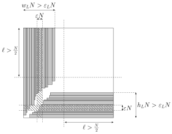
(a) Packing of $L$-region using rectangles from $OPT_{\mathrm{long}}$. Striped strips are cheapest $\varepsilon N$-width and cheapest $\varepsilon N$-height.

(b) Packing of rectangles in $OPT_{\mathrm{long}}\cup(OPT_{\mathrm{short}}\cap OPT_{T})$. Dark gray rectangles are from $OPT_{\mathrm{short}}\cap OPT_{T}$.

Figure 4.8: The case for $w_{L}>\varepsilon_{L}$ and $h_{L}>\varepsilon_{L}$.

(a) Packing of $L$-region using rectangles from $OPT_{\mathrm{long}}$. Striped strip is the cheapest $\varepsilon N$-width strip.

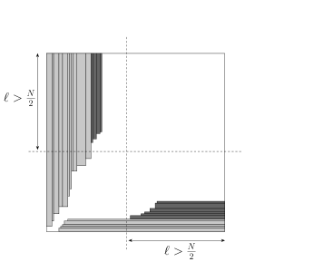
(b) Packing of rectangles in $OPT_{\mathrm{long}}\cup(OPT_{\mathrm{short}}\cap OPT_{T})$. Dark gray rectangles are from $OPT_{\mathrm{short}}\cap OPT_{T}$.

Figure 4.9: The case for $w_{L}>\varepsilon_{L}$ and $h_{L}\leq\varepsilon_{L}$.

Packing of subset of rectangles from $OPT_{\mathrm{long}}\cup(OPT_{\mathrm{short}}\cap OPT_{T})$ into $L$-region.
If ($w_{L}>\varepsilon_{L}$ and $h_{L}>\varepsilon_{L}$), we partition the vertical part of the $L$-region into consecutive strips of width $\varepsilon N$. Consider the strip that intersects the least number of vertical rectangles from $OPT_{\mathrm{long}}$ among all strips, and we call it to be the cheapest $\varepsilon N$-width vertical strip (See Figure 4.8(a)). Clearly the cheapest $\varepsilon N$-width vertical strip intersects at most a $\frac{\varepsilon+2\varepsilon_{small}}{\varepsilon_{L}}\leq O(\varepsilon_{L})$ fraction of the rectangles in the vertical part of $L$-region, so we can remove all such vertical rectangles intersected by the cheapest $\varepsilon N$-width vertical strip at a small loss of profit. Similarly, we remove the horizontal rectangles intersected by the cheapest $\varepsilon N$-height horizontal strip in the boundary $L$-region and push the remaining rectangles in the $L$ region to the bottom and left. We now pack the horizontal container for $OPT_{\mathrm{short}}\cap OPT_{T}$ above the horizontal part of $L$ region and the vertical container for $OPT_{\mathrm{short}}\cap OPT_{T}$ to the right of the vertical part of the $L$-region (See Figure 4.8(b)).
In the other case ($w_{L}>\varepsilon_{L},h_{L}\leq\varepsilon_{L}$ and $w(V_{1-2\varepsilon_{L}})\leq\left(\frac{1}{2}-2\varepsilon_{large}\right)N$), we can again remove the cheapest $\varepsilon N$-width vertical strip in the boundary $L$-region and pack the vertical container for $OPT_{\mathrm{short}}\cap OPT_{T}$ there (See Figure 4.9(a)). Now we show how to pack horizontal items from $OPT_{\mathrm{short}}\cap OPT_{T}$. In the packing of the boundary $L$-region, we can assume that the vertical rectangles are sorted non-increasingly by height from left to right and pushed upwards until they touch the top boundary. Then, since $w(V_{1-2\varepsilon_{L}})\leq\left(\frac{1}{2}-2\varepsilon_{large}\right)N$ and ($h_{L}\leq\varepsilon_{L}$), the region $\left[\left(\frac{1}{2}-2\varepsilon_{large}\right)N,N\right]\times\left[\varepsilon_{L}N,2\varepsilon_{L}N\right]$ will be completely empty and thus we will have enough space to pack the horizontal container for $OPT_{\mathrm{short}}\cap OPT_{T}$ on top of the horizontal part of the $L$-region (See Figure 4.9(b)). The last case, when $w_{L}\leq\varepsilon_{L}$, is analogous. Thus we have a packing in boundary $L$-region of width at most $(w_{L}+\varepsilon_{L})N$ and height at most $(h_{L}+\varepsilon_{L})N$ with total profit at least $\frac{3(1-O(\varepsilon))}{4}(|OPT_{\mathrm{long}}|)+|OPT_{\mathrm{short}}\cap OPT_{T}|$, implying that

$$|OPT_{L\&C}|\geq\frac{3(1-O(\varepsilon))}{4}(|OPT_{\mathrm{long}}|)+|OPT_{\mathrm{short}}\cap OPT_{T}|$$ (4.8)

Packing of subset of rectangles from $OPT_{\mathrm{short}}\setminus OPT_{T}$ into the remaining region.
Note that after packing rectangles of cardinality at least $\frac{3(1-O(\varepsilon))}{4}|OPT_{\mathrm{long}}|+|OPT_{\mathrm{short}}\cap OPT_{T}|$ in the boundary $L$-region, the remaining rectangular region, let us call it to be $\mathcal{R}_{container}$, of width $(1-w_{L}-\varepsilon_{L})N$ and height $(1-h_{L}-\varepsilon_{L})N$ is completely empty. Now we will show the existence of a packing of some rectangles from $OPT_{\mathrm{short}}\setminus OPT_{T}$ in the remaining space of the packing (even using some space from the $L$-boundary region). Let $(OPT_{\mathrm{short}}\setminus OPT_{T})_{hor}:=(OPT_{\mathrm{short}}\setminus OPT_{T})\cap R_{hor}$ and $(OPT_{\mathrm{short}}\setminus OPT_{T})_{ver}:=(OPT_{\mathrm{short}}\setminus OPT_{T})\cap R_{ver}$. Let us assume without loss of generality that vertical rectangles are shifted as much as possible to the left and top of the knapsack and horizontal are pushed as much as possible to the right and bottom. We divide the analysis in three subcases depending on $a(OPT_{\mathrm{short}}\setminus OPT_{T})$.
$-$ Subcase (i). If $a(OPT_{\mathrm{short}}\setminus OPT_{T})\leq\frac{3}{5}N^{2}$, from inequalities (4.2), (4.3), (4.4), (4.8) and Lemma 69 we get

$$|OPT_{L\&C}|\geq\left(\frac{127}{216}-O(\varepsilon_{L})\right)|OPT|$$ (4.9)

$-$ Subcase (ii). If $a(OPT_{\mathrm{short}}\setminus OPT_{T})>(\frac{3}{4}+\varepsilon+\varepsilon_{large})N^{2}$, from inequalities (4.2), (4.3), (4.4), (4.8) and Lemma 70 we get

$$|OPT_{L\&C}|\geq\left(\frac{17}{28}-O(\varepsilon_{L})\right)|OPT|$$ (4.10)

$-$ Subcase (iii). Finally, if $\frac{3}{5}N^{2}\leq a(OPT_{\mathrm{short}}\setminus OPT_{T})\leq(\frac{3}{4}+\varepsilon+\varepsilon_{large})N^{2}$, from inequality (4.5) we get, $\alpha+\beta\leq 2(1-\frac{3}{5})\leq\frac{4}{5}$. Now we consider two subcases.
$\odot$ Subcase (iii a): $w_{L}\leq\frac{1}{2}$ and $h_{L}\leq\frac{1}{2}$. Note that in this case if $w_{L}\geq\frac{1}{2}-2\varepsilon_{large}-2\varepsilon_{L}$ or $h_{L}\geq\frac{1}{2}-2\varepsilon_{large}-2\varepsilon_{L}$, we can remove the cheapest $2(\varepsilon_{L}+\varepsilon_{large})N$-width vertical strip and the cheapest $2(\varepsilon_{L}+\varepsilon_{large})N$-height horizontal strip from the $L$-region. Otherwise we have $w_{L}<\frac{1}{2}-2\varepsilon_{large}-2\varepsilon_{L}$ and $h_{L}<\frac{1}{2}-2\varepsilon_{large}-2\varepsilon_{L}$. So there is free rectangular region that has both side lengths at least $N(\frac{1}{2}+2\varepsilon_{large}+\varepsilon_{L})$; we will keep $\varepsilon_{L}N$ width and $\varepsilon_{L}N$ height for resource augmentation and use the rest of the rectangular region (with both sides length at least $\left(\frac{1}{2}+2\varepsilon_{large}\right)N$) for showing existence of a packing using Steinberg’s theorem. Note that this rectangular region has area at least $N^{2}(1-w_{L}-2\varepsilon_{L})(1-h_{L}-2\varepsilon_{L})$. Thus by using Steinberg’s theorem, we can pack either rectangles from $(OPT_{\mathrm{short}}\setminus OPT_{T})_{hor}$ (by sorting them non-decreasingly by area and picking them iteratively) having total area at least $min\{a((OPT_{\mathrm{short}}\setminus OPT_{T})_{hor}),\frac{N^{2}(1-w_{L}-2\varepsilon_{L})(1-h_{L}-2\varepsilon_{L})}{2}-\varepsilon_{small}\}$ or rectangles from $(OPT_{\mathrm{short}}\setminus OPT_{T})_{ver}$ with total area at least $min\{a((OPT_{\mathrm{short}}\setminus OPT_{T})_{ver}),\frac{N^{2}(1-w_{L}-2\varepsilon_{L})(1-h_{L}-2\varepsilon_{L})}{2}-\varepsilon_{small}\}$. We claim that if we keep the best of the two packings, we can always pack at least $\left(\frac{7}{48}-O(\varepsilon_{L})\right)|OPT_{\mathrm{short}}\setminus OPT_{T}|$. Note that it is sufficient to consider, $\frac{N^{2}(1-w_{L}-O(\varepsilon_{L}))(1-h_{L}-O(\varepsilon_{L}))}{2}<\min\{a((OPT_{\mathrm{short}}\setminus OPT_{T})_{hor}),a((OPT_{\mathrm{short}}\setminus OPT_{T})_{ver})\}$, as otherwise, we can pack even more rectangles from $OPT_{\mathrm{short}}\setminus OPT_{T}$ than the claimed fraction. In this case, we pack at least

$$\geq \frac{N^{2}}{2}\left(\frac{(1-w_{L}-O(\varepsilon_{L}))(1-h_{L}-O(\varepsilon_{L}))}{2a(OPT_{\mathrm{short}}\setminus OPT_{T})}|OPT_{\mathrm{short}}\setminus OPT_{T}|\right)$$

where the inequality follows from the fact that $\frac{a}{b}+\frac{c}{d}\geq\frac{(a+c)}{(b+d)}$ for $a,b,c,d\geq 0$. Since $a(OPT_{\mathrm{short}}\setminus OPT_{T})\leq(1-\frac{\alpha}{2}-\frac{\beta}{2})N^{2}\leq(1-\frac{w_{L}}{2}-\frac{h_{L}}{2})N^{2}$ and $w_{L}+h_{L}\leq\alpha+\beta\leq\frac{4}{5}$, we can minimize the expression

$$\frac{1}{2}\left(\frac{N^{2}(1-w_{L}-O(\varepsilon_{L}))(1-h_{L}-O(\varepsilon_{L}))}{2a(SF)}|OPT_{\mathrm{short}}\setminus OPT_{T}|\right)$$

over the domain $\{w_{L}+h_{L}\leq\frac{4}{5},0\leq w_{L}\leq\frac{1}{2},0\leq h_{L}\leq\frac{1}{2}\}$, obtaining that this is at least $(\frac{7}{48}-O(\varepsilon_{L}))|OPT_{\mathrm{short}}\setminus OPT_{T}|$ (value reached at $w_{L}=\frac{1}{2}$ and $h_{L}=\frac{3}{10}$). This together with inequalities (4.2), (4.3), (4.4), (4.8) and Lemma 69 implies that

$$|OPT_{L\&C}|\geq\left(\frac{215}{369}-O(\varepsilon_{L})\right)|OPT|$$ (4.11)

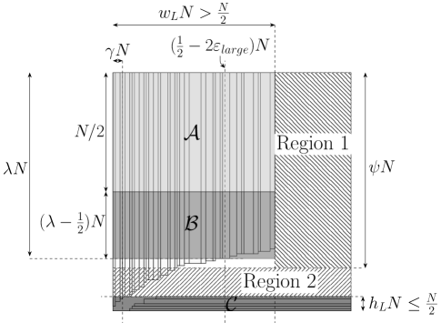
Figure 4.10: Case 2A(iii)b in the proof of Theorem 66

$\odot$ Subcase (iii b): $w_{L}>\frac{1}{2}$ (then from inequality (4.5), $h_{L}\leq\frac{3}{10}$). Note that $a(OPT_{\mathrm{long}})\leq(1-\frac{3}{5})N^{2}=\frac{2}{5}N^{2}$.
Let us define some parameters from the current packing to simplify the calculations. Let $\lambda N$ be the height of the tallest vertical rectangle in the packing that touches the vertical line $x=\left(\frac{1}{2}-2\varepsilon_{large}\right)N$ and $\gamma N$ be the total width of vertical rectangles having height greater than $(1-h_{L})N$. We define also the following three regions in the knapsack: $\mathcal{A}$, the rectangular region of width $w_{L}N$ and height $\frac{1}{2}N$ in the top left corner of the knapsack; $\mathcal{B}$, the rectangular region of width $w_{L}N$ and height $(\lambda-\frac{1}{2})N$ below $\mathcal{A}$ and left-aligned with the knapsack; and $\mathcal{C}$, the rectangular region of width $N$ and height $h_{L}N$ touching the bottom boundary of the knapsack. Notice that $\mathcal{A}$ is fully occupied by vertical rectangles, $\mathcal{B}$ is almost fully occupied by vertical rectangles except for the right region of width $w_{L}N-\left(\frac{1}{2}-2\varepsilon_{large}\right)N$, and at least half of $\mathcal{C}$ is occupied by horizontal rectangles (some vertical rectangles may overlap with this region). Our goal is to pack some rectangles from $OPT_{\mathrm{short}}\setminus OPT_{T}$ in the L -shaped region outside $\mathcal{A}\cup\mathcal{B}\cup\mathcal{C}$. Let $\psi\in[\lambda,1-h_{L}]$ be a parameter to be fixed. We will use, when possible, the following regions for packing items from $OPT_{\mathrm{short}}\setminus OPT_{T}$: Region 1 on the top right corner of the knapsack with width $N(1-w_{L})$ and height $\psi N$ and Region 2 which is the rectangular region $[0,N]\times[h_{L}N,(1-\psi)\cdot N]$ (see Figure 4.10). Region $1$ is completely free but Region 2 may overlap with vertical rectangles.

We will now divide Region 2 into a constant number of boxes such that: they do not overlap with vertical rectangles, the total area inside Region 2 which is neither overlapping with vertical rectangles nor covered by boxes is at most $O(\varepsilon_{L})N^{2}$ and each box has width at least $\left(\frac{1}{2}+2\varepsilon_{large}\right)N$ and height at least $\varepsilon N$. That way we will be able to pack rectangles from $(OPT_{\mathrm{short}}\setminus OPT_{T})_{ver}$ into the box defined by Region $1$ and rectangles from $(OPT_{\mathrm{short}}\setminus OPT_{T})_{hor}$ into the boxes defined inside Region 2 using almost completely its free space. In order to create the boxes inside Region 2 we first create a monotone chain by doing the following: Let $(x_{1},y_{1})=(\gamma N,h_{L})$. Starting from position $(x_{1},y_{1})$, we draw an horizontal line of length $\varepsilon_{L}N$ and then a vertical line from bottom to top until it touches a vertical rectangle, reaching position $(x_{2},y_{2})$. From $(x_{2},y_{2})$ we start again the same procedure and iterate until we reach the vertical line $x=\left(\frac{1}{2}-2\varepsilon_{large}\right)N$ or the horizontal line $y=(1-\psi)N$. Notice that the area above the monotone chain and below $y=(1-\psi)N$ that is not occupied by vertical rectangles, is at most $\sum_{i}{\varepsilon_{L}N(y_{i+1}-y_{i})}\leq\varepsilon_{L}N^{2}$. The number of points $(x_{i},y_{i})$ defined in the previous procedure is at most $1/\varepsilon_{L}$. By drawing an horizontal line starting from each $(x_{i},y_{i})$ up to $(N,y_{i})$, together with the drawn lines from the monotone chain and the right limit of the knapsack, we define $k\leq 1/\varepsilon_{L}$ boxes. We discard the boxes having height less than $\varepsilon N$, whose total area is at most $\frac{\varepsilon}{\varepsilon_{L}}N^{2}\leq\varepsilon_{L}N^{2}$, and have all the desired properties for the boxes.

Since the total area of rectangles in $OPT_{\mathrm{long}}$ is at most $\frac{2}{5}N^{2}$, the total area not occupied by boxes in Region 2 is at most $N^{2}(\frac{2}{5}-\frac{1}{2}w_{L}-(\lambda-\frac{1}{2})\frac{1}{2}-\frac{1}{2}h_{L})=N^{2}(\frac{13}{20}-\frac{w_{L}}{2}-\frac{\lambda}{2}-\frac{h_{L}}{2})$, which comes from the area we know is occupied for sure in regions $\mathcal{A},\mathcal{B}$ and $\mathcal{C}$ by rectangles in $OPT_{\mathrm{long}}$. This implies that the total area of the horizontal boxes is at least $N^{2}(1-\psi-h_{L})-N^{2}(\frac{13}{20}-\frac{w_{L}}{2}-\frac{\lambda}{2}-\frac{h_{L}}{2})$ and the area of the vertical box is $(1-w_{L})\psi$. These two areas become equal if we can set $\psi=\frac{7+10(w_{L}+\lambda-h_{L})}{40-20w_{L}}$. It is not difficult to verify that in this case $\psi\leq 1-h_{L}$. If $\frac{7+10(w_{L}+\lambda-h_{L})}{40-20w_{L}}\geq\lambda$, then we set $\psi=\frac{7+10(w_{L}+\lambda-h_{L})}{40-20w_{L}}$. Otherwise we set $\psi=\lambda$.

First, consider when $\psi=\frac{7+10(w_{L}+\lambda-h_{L})}{40-20w_{L}}$. Since $\psi\geq\lambda$, the width of the boxes inside Region 2 is at least $\left(\frac{1}{2}+2\varepsilon_{large}\right)N$ and the box in Region $1$ has height at least $\left(\frac{1}{2}+2\varepsilon_{large}\right)N$. By using Steinberg’s theorem, we can always pack in these boxes at least

Note that from each box $B^{\prime}$ of height $h(\geq\varepsilon N)$, we can remove the cheapest $\varepsilon h$-horizontal strip and use resource augmentation to get a container based packing with nearly the same profit as $B^{\prime}$. Thus by performing a similar analysis to the one done in Subcase (iii a), and using the fact that $a(OPT_{\mathrm{short}}\setminus OPT_{T})\leq N^{2}-(\frac{\alpha}{2}+(\lambda-\frac{1}{2})\frac{1}{2}+\frac{\beta}{2})N^{2}\leq N^{2}-N^{2}(\frac{w_{L}}{2}+(\lambda-\frac{1}{2})\frac{1}{2}+\frac{h_{L}}{2})$, we can minimize the whole expression over the domain $\{\frac{w_{L}}{2}+(\lambda-\frac{1}{2})\frac{1}{2}+\frac{h_{L}}{2}\leq\frac{2}{5},\frac{1}{2}\leq w_{L}\leq\frac{4}{5},\frac{1}{2}\leq\lambda\leq 1,0\leq\beta\leq\frac{1}{2}\}$ and prove that this solution packs at least

$$\left(\frac{3-O(\varepsilon_{L})}{4}\right)|OPT_{\mathrm{long}}|+|OPT_{\mathrm{short}}\cap OPT_{T}|+\left(\frac{5}{36}-O(\varepsilon_{L})\right)|OPT_{\mathrm{short}}\setminus OPT_{T}|.$$

Thus, using the above inequality along with (4.2), (4.3), (4.4) and Lemma 69, we get

$$|OPT_{L\&C}|\geq\left(\frac{325}{558}-O(\varepsilon_{L})\right)|OPT|$$ (4.12)

Finally, if $\psi=\lambda<\frac{7+10(w_{L}+\lambda-h_{L})}{40-20w_{L}}$, we will not get equal area horizontal and vertical boxes for packing of items in $OPT_{\mathrm{short}}\setminus OPT_{T}$. In this case we change the width of the box inside Region $1$ to be $w_{L}^{\prime}<N(1-w_{L})$ fixed in such a way that the area of this box is equal to the bound we have for the area of the boxes in Region $2$, i.e., $N^{2}(1-\lambda-h_{L})-(\frac{13}{20}-\frac{w_{L}}{2}-\frac{h_{L}}{2}-\frac{\lambda}{2}+O(\varepsilon_{L}))N^{2}$. Performing the same analysis as before, it can be shown that in this case we pack at least

$$\left(\frac{(1-\lambda-h_{L})N^{2}-(\frac{13}{20}-\frac{w_{L}}{2}-\frac{h_{L}}{2}-\frac{\lambda}{2})N^{2}}{2a(OPT_{\mathrm{short}}\setminus OPT_{T})}-O(\varepsilon_{L})\right)|OPT_{\mathrm{short}}\setminus OPT_{T}|,$$

which is at least $(\frac{1}{6}-O(\varepsilon_{L}))|OPT_{\mathrm{short}}\setminus OPT_{T}|$ over the domain $\{\frac{w_{L}}{2}+(\lambda-\frac{1}{2})\frac{1}{2}+\frac{h_{L}}{2}\leq\frac{2}{5},\psi<\lambda,\frac{1}{2}\leq w_{L}\leq\frac{4}{5},\frac{1}{2}\leq\lambda\leq 1,0\leq\beta\leq\frac{3}{10}\}$ (and this solution is then better than (4.12)).

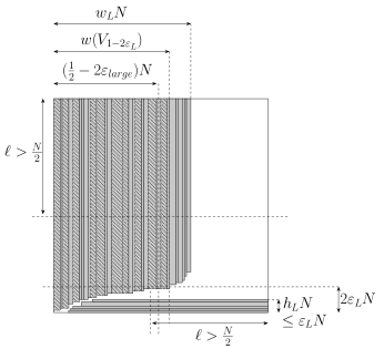
(a) Packing of $L$-region using rectangles from $OPT_{\mathrm{long}}$. Striped rectangles are removed.

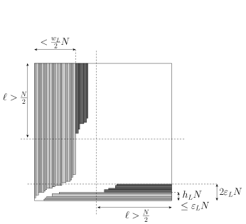
(b) Packing of rectangles in $OPT_{\mathrm{long}}\cup(OPT_{\mathrm{short}}\cap OPT_{T})$. Dark gray rectangles are from $OPT_{\mathrm{short}}\cap OPT_{T}$.

Figure 4.11: The case 2B.

$\Diamond$ Case 2B. ($h_{L}<\varepsilon_{L}$ and $w(V_{1-2\varepsilon_{L}})>\left(\frac{1}{2}-2\varepsilon_{large}\right)N$) or ($w_{L}<\varepsilon_{L}$ and $h(H_{1-2\varepsilon_{L}})>\left(\frac{1}{2}-2\varepsilon_{large}\right)N$)
In the first case $a(OPT_{\mathrm{long}})>\left(\frac{1}{2}-2\varepsilon_{large}\right)(1-2\varepsilon_{L})N^{2}+(w_{L}-\frac{1}{2})N\cdot\frac{N}{2}\geq(\frac{1}{4}+\frac{w_{L}}{2}-\varepsilon_{L}-2\varepsilon_{large})N^{2}$. Thus $a(OPT_{\mathrm{short}}\setminus OPT_{T})<(\frac{3}{4}-\frac{w_{L}}{2}+\varepsilon_{L}+2\varepsilon_{large})N^{2}$.
Now consider the vertical rectangles in the boundary $L$-region sorted non-increasingly by width and pick them iteratively until their total width crosses $(\frac{w_{L}}{2}+3\varepsilon_{L}+2\varepsilon_{large})N$. Remove these rectangles and push the remaining vertical rectangles in the $L$-region to the left as much as possible. This modified $L$-region will have profit at least $(\frac{1}{2}-O(\varepsilon_{L}))|OPT_{\mathrm{long}}|$. Now we can put $\varepsilon N$-strip for the vertical items from $OPT_{\mathrm{short}}\cap OPT_{T}$ next to the vertical part of $L$-region. On the other hand, horizontal part of $OPT_{\mathrm{short}}\cap OPT_{T}$ can be placed on top of horizontal part of $L$-region. The remaining space will be a free rectangular region of height at least $(1-2\varepsilon_{L})N$ and width $(1-\frac{w_{L}}{2}+2\varepsilon_{L}+2\varepsilon_{large})N$. We will use a part of this rectangular region of height $(1-3\varepsilon_{L})N$ and width $(1-\frac{w_{L}}{2}+\varepsilon_{L})N$ to pack rectangles from $OPT_{\mathrm{short}}\setminus OPT_{T}$ and the rest of the region for resource augmentation. Using Lemma 68, we can pack small rectangles in this region with profit at least $\Big{(}\frac{(1-\frac{w_{L}}{2})/2}{\frac{3}{4}-\frac{w_{L}}{2}}-O(\varepsilon_{L})\Big{)}|OPT_{\mathrm{short}}\setminus OPT_{T}|\geq(\frac{3}{4}-O(\varepsilon_{L}))|OPT_{\mathrm{short}}\setminus OPT_{T}|$ as $w_{L}\geq\frac{1}{2}$. Hence, we get,

$$|OPT_{L\&C}| \geq\left(\frac{1}{2}-O(\varepsilon_{L})\right)|OPT_{\mathrm{long}}|+|OPT_{\mathrm{short}}\cap OPT_{T}|$$ (4.13)

$$\quad+\left(\frac{3}{4}-O(\varepsilon_{L})\right)|OPT_{\mathrm{short}}\setminus OPT_{T}|$$

On the other hand, as $a(OPT_{\mathrm{short}}\setminus OPT_{T})\leq(\frac{3}{4}-\frac{w_{L}}{2}+\varepsilon_{L}+2\varepsilon_{large})N^{2}$ and $w_{L}>1/2$, we get $a(OPT_{\mathrm{short}}\setminus OPT_{T})\leq\frac{1}{2}N^{2}$ and thus from Lemma 69 we get,

$$|OPT_{L\&C}|\geq\frac{3}{4}|OPT_{\mathrm{long}}\cap OPT_{T}|+(1-O(\varepsilon_{L}))|OPT_{\mathrm{short}}|$$ (4.14)

From inequalities (4.1), (4.3), (4.4), (4.13), (4.14), we get,

$$|OPT_{L\&C}|\geq\left(\frac{24}{41}-O(\varepsilon_{L})\right)|OPT|$$ (4.15)

Now we consider the last case when $w_{L}<\varepsilon_{L}$ and $h(H_{1-2\varepsilon_{L}})>\left(\frac{1}{2}-2\varepsilon_{large}\right)N$. Note that as we assumed the cheapest subring was the top subring, after removing it we might be left with only $|OPT_{\mathrm{long}}\cap R_{hor}|/2$ profit in the horizontal part of $L$-region. So, further removal of items from the horizontal part might not give us a good solution. Thus we show an alternate good packing. We restart with the ring packing and delete the cheapest vertical subring instead of the cheapest subring (i.e., the top subring) and create a new boundary $L$-region. Here, consider the horizontal rectangles in the boundary $L$-region in non-increasing order of height and take them until their total height crosses $(\frac{\beta_{1}+\beta_{2}}{2}+\varepsilon_{small}+\varepsilon)N$. Remove these rectangles and push the remaining horizontal rectangles to the bottom as much as possible. Then, following similar arguments as in case 2B, we will obtain the same bounds as in inequality (4.15).

In summary, from all the cases (see Figure 4.7 for the overview of the case analysis) the profit of the obtained solution is at least

$$\left(\frac{325}{558}-O(\varepsilon_{L})\right)|OPT|.$$

∎

4.5 Conclusions

In this chapter, we presented techniques for 2DGK that are not entirely based on containers. By leveraging a combination of container packings and L-packings, we obtained the first algorithm that break the barrier of $2$ for the approximation factor of this problem. We obtained an approximation factor of $17/9+\varepsilon<1.89$ for the weighted case, and $\frac{558}{325}+\varepsilon<1.72$ in the cardinality case.

Further improvements could come from the study of generalizations of L-packings. For example, a PTAS for ring-packing instances arising by shifting of long items would lead to an improved approximation factor. A PTAS for $O(1)$ simultaneous L-packings would also be an interesting development, and might be a stepping stone for the long-standing problem of finding a PTAS for 2DGK, which remains open even in the cardinality case, and even if pseudo-polynomial time is allowed instead of polynomial time.

Chapter 5 Approximations for 2DGK
with Rotations

In this chapter, we consider the 2DGKR problem, where we are allowed to rotate the rectangles by $90^{\circ}$.

The possibility to rotate the rectangles makes the problem significantly easier. In fact, we obtain better approximation factors, and we do not need L-packings anymore, obtaining purely container-based algorithms.

The basic idea is that any thin item can now be packed inside a narrow vertical strip (say at the right edge of the knapsack) by possibly rotating it. This way we do not lose one quarter of the profit due to the mapping to an L-packing and instead place all items from the ring into the mentioned strip (while we ensure that their total width is small). The remaining short items are packed by means of a novel resource contraction lemma: unless there is one huge item that occupies almost the whole knapsack (a case that we consider separately), we can pack almost one half of the profit of non-thin items in a reduced knapsack where one of the two sides is shortened by a factor $1-\varepsilon$ (hence leaving enough space for the vertical strip). Thus, roughly speaking, we obtain either all profit of non-thin items, or all profit of thin items plus one half of the profit of non-thin items: this gives a $3/2+\varepsilon$ approximation. A further refinement of this approach yields a $4/3+\varepsilon$ approximation in the cardinality case. We remark that, while resource augmentation is a well-established notion in approximation algorithms, resource contraction seems to be a rather novel direction to explore.

Theorem 71.

For any constant $\varepsilon>0$, there exists a polynomial-time $\frac{3}{2}+\varepsilon$ approximation algorithm for 2DGKR. In the cardinality case the approximation factor can be improved to $\frac{4}{3}+\varepsilon$.

First, let us introduce some notations. Without loss of generality, assume $0pt(i)\geq 0pt(i)$ for all rectangles $R_{i}\in\mathcal{R}$. Now consider packing of some optimal solution in the knapsack. Denote the strips of width $N$ and height $\varepsilon N$ at the top and bottom of the knapsack by $S_{T,\varepsilon}:=[0,N]\times[(1-\varepsilon)N,N]$ and $S_{B,\varepsilon}:=[0,N]\times[0,\varepsilon N]$. Similarly, denote the strips of height $N$ and width $\varepsilon N$ to the left and right of the bin by $S_{L,\varepsilon}:=[0,\varepsilon N]\times[0,N]$ and $S_{R,\varepsilon}:=[(1-\varepsilon)N,N]\times[0,N]$. The set of rectangles intersected by one of these strips $S_{K,\varepsilon},K\in\{T,B,L,R\}$ is denoted by $E_{K,\varepsilon}$. There are two kinds of rectangles that intersect these strips. The set of rectangles completely contained inside one of these strips $S_{K,\varepsilon}$, is denoted by $C_{K,\varepsilon}$. The set of remaining rectangles that do not lie completely inside the strip $S_{K,\varepsilon}$ but intersect the strip, is denoted by $D_{K,\varepsilon}$ (see Figure 5.3). With slight abuse of notations, we will assume $C_{K,\varepsilon}$ also represents the embedding of corresponding rectangles in the strip.

5.1 Weighted Case

In this section we give a polynomial time $(3/2+\varepsilon)$-approximation algorithm for the weighted 2-dimensional geometric knapsack problem when items are allowed to be rotated by $90^{\circ}$. In contrary to the unweighted case, where it is possible to remove a constant number of large items, the same is not possible in the weighted case, where an item could have a big profit.

We call an item $i$ massive if $0pt(i)\geq(1-\varepsilon)N$ and $0pt(i)\geq(1-\varepsilon)N$. The presence of such a big item in the optimal solution requires a different analysis, that we present below. In both the cases, we can show that there exists a container packing with roughly 2/3 of the profit of the optimal solution.

Let us assume that $\varepsilon<1/6$. We will prove the following result:

Theorem 72.

Let $\varepsilon>0$ and let $\mathcal{R}$ be a set of items that can be packed into the $N\times N$ knapsack. Then there exists an $\varepsilon$-granular container packing with $O_{\varepsilon}(1)$ containers of a subset $\mathcal{R}^{\prime}\subseteq\mathcal{R}$ into the $N\times N$ knapsack such that $p(\mathcal{R}^{\prime})\geq(2/3-O(\varepsilon))p(\mathcal{R})$, if rotations are allowed.

We start by analyzing the case of a set $\mathcal{R}$ that has a massive item.

Lemma 73.

Suppose that a set $\mathcal{R}$ of items can be packed into a $N\times N$ bin and there is a massive item $m\in\mathcal{R}$. Then, there is a container packing with at most $O_{\varepsilon}(1)$ containers for a subset $\mathcal{R}^{\prime}\subseteq\mathcal{R}$ such that $p(\mathcal{R}^{\prime})\geq\left(\dfrac{2}{3}-O(\varepsilon)\right)p(\mathcal{R})$.

Proof.

Assume, without loss of generality, that $1/(3\varepsilon)$ is an integer. Consider the items in $\mathcal{R}\setminus\{m\}$. Clearly, each of them has width or height at most $\varepsilon$; moreover, $a(\mathcal{R}\setminus\{m\})\leq(1-(1-\varepsilon)^{2})N^{2}=(2\varepsilon-\varepsilon^{2})N^{2}\leq\frac{N^{2}}{2(1+\varepsilon)}$, as $\varepsilon<1/6$; thus, by possibly rotating each element so that the height is smaller than $\varepsilon$, by Theorem 3 all the items in $\mathcal{R}\setminus\{m\}$ can be packed in a $N\times\frac{N}{1+\varepsilon}$ bin; then, by Lemma 14, there is a container packing for a subset of $\mathcal{R}\setminus\{m\}$ with $O_{\varepsilon}(1)$ containers that fits in the $N\times N$ bin and has profit at least $(1-O(\varepsilon))p(\mathcal{R}\setminus\{m\})$

Consider now the packing of $\mathcal{R}$. Clearly, the region $[\varepsilon N,(1-\varepsilon)N]^{2}$ is entirely contained within the boundaries of the massive item $m$. Partition the region with $x$-coordinate between $\varepsilon N$ and $(1-\varepsilon)N$ in $k=1/(3\varepsilon)$ strips of width $3\varepsilon(1-2\varepsilon)N\geq 2\varepsilon N$ and height $N$, let them be $S_{1},\dots,S_{k}$; let $\mathcal{R}(S_{i})$ be the set of items in $\mathcal{R}$ such that their left or right edge (or both) are contained in the interior of strip $S_{i}$. Since each item belongs to at most two of these sets, there exists $i$ such that $p(\mathcal{R}(S_{i}))\leq 6\varepsilon p(\mathcal{R})$.
Symmetrically, we define $k$ horizontal strips $T_{1},\dots,T_{k}$, obtaining an index $j$ such that $p(\mathcal{R}(T_{j}))\leq 6\varepsilon p(\mathcal{R})$. Thus, no item in $\overline{\mathcal{R}}:=\mathcal{R}\setminus(R(S_{i})\cup R(T_{j}))$ has a side contained in the interior of $S_{i}$ or $T_{j}$, and $p(\overline{\mathcal{R}})\geq(1-12\varepsilon)p(\mathcal{R})$. Let $M_{V}$ be the set of items in $\overline{\mathcal{R}}\setminus\{m\}$ that overlap $T_{j}$, and let $M_{H}$ be the set of items in $\overline{\mathcal{R}}\setminus\{m\}$ that overlap $S_{i}$. Clearly, the items in $M_{H}$ can be packed in a horizontal container with width $N$ and height $N-0pt(m)$, and the items in $M_{V}$ can be packed in a vertical container of width $N-0pt(m)$ and height $N$.

Let $H$ be the set of items of $\overline{\mathcal{R}}\setminus M_{H}$ that are completely above the massive item $m$ or completely below it; symmetrically, let $V$ be the set of items of $\overline{\mathcal{R}}\setminus M_{V}$ that are completely to the left or completely to the right of $m$. We will now show that there is a container packing for $M_{H}\cup V\cup\{m\}$. Since all the elements overlapping $T_{j}$ have been removed, $V$ can be packed in a bin of size $(N-0pt(m))\times(1-2\varepsilon)N$ (see Figure 5.1). Since $(1-2\varepsilon)N\cdot(1+\varepsilon)<(1-\varepsilon)N\leq 0pt(m)$, Lemma 14 implies that there is a container packing of a subset of $V$ with profit at least $(1-O(\varepsilon))p(V)$ in a bin of size $(N-0pt(m))\times 0pt(m)$ and using $O_{\varepsilon}(1)$ containers; thus, by adding a horizontal container of the same size as $m$ and a horizontal container of size $N\times(N-0pt(m))$, we obtain a container packing for $M_{H}\cup V\cup\{m\}$ with $O_{\varepsilon}(1)$ containers and profit at least $(1-O(\varepsilon))p(M_{H}\cup V\cup\{m\})$. Symmetrically, there is a container packing for a subset of $M_{V}\cup H\cup\{m\}$ with profit at least $(1-O(\varepsilon))p(M_{V}\cup H\cup\{m\})$ and $O_{\varepsilon}(1)$ containers.

Let $\mathcal{R}_{MAX}$ be the set of maximum profit among the sets $\mathcal{R}\setminus\{m\}$, $M_{H}\cup V\cup\{m\}$ and $M_{V}\cup H\cup\{m\}$. By the discussion above, there is a container packing for $\mathcal{R}^{\prime}\subseteq\mathcal{R}_{MAX}$ with $O_{\varepsilon}(1)$ containers and profit at least $(1-O(\varepsilon))p(\mathcal{R}_{MAX})$. Since each element in $\overline{\mathcal{R}}$ is contained in at least two of the above three sets, it follows that:

$$p(\mathcal{R}^{\prime}) \geq(1-O(\varepsilon))p(\mathcal{R}_{MAX})\geq\left(1-O(\varepsilon)\right)\left(\frac{2}{3}p(\overline{\mathcal{R}})\right)$$

$$\geq\left(\frac{2}{3}-O(\varepsilon)\right)p(\mathcal{R})$$

∎

(a) Massive item case. Items intersecting strips $M_{H}$ and $M_{V}$ (hatched rectangles) cross them completely.
 

(b) $Bottom(i),Top(i),Left(i),Right(i)$ are represented by vertical, horizontal, north east and north west stripes respectively.

Figure 5.1:

If there is no massive item, we will show existence of two container packings and show the maximum of them always packs items with total profit at least $\left(\frac{2}{3}-O(\varepsilon)\right)$ fraction of the optimal profit.

First, we follow the corridor decomposition and the classification of items as in Section 4.3 to define sets $LF,SF,LT,ST,OPT_{small}$. Let $T:=LT\cup ST$ be the set of thin items. Also let $APX$ be the best container packing and $OPT$ be the optimal solution. Then similar to Lemma 64, we can show $p(APX)\geq(1-\varepsilon)(p(LF)+p(SF)+p(OPT_{small}))$. Thus,

$$p(APX)\geq(1-\varepsilon)p(OPT)-p(T).$$ (5.1)

In the second case, we define the set $T$ as above. Then in Resource Contraction Lemma (Lemma 74), we will show that one can pack $1/2$ of the remaining profit in the optimal solution, i.e., $p(OPT\setminus T)/2$ in a knapsack of size $N\times(1-\varepsilon/2)N$. Now, we can pack $T$ in a horizontal container of height $\varepsilon/4$ and using Lemma 74 and resource augmentation we can pack $p(OPT\setminus T)/2$ in the remaining space $N\times(1-\varepsilon/4)N$. Thus,

$$p(APX)\geq p(T)+(1-\varepsilon)(p(OPT)-p(T))/2.$$ (5.2)

Hence, up to $(1-O(\varepsilon))$ factor, we obtain a packing with profit at least $\max\{(p(T)+p(OPT\setminus T)/2),p(OPT\setminus T)\}\geq 2/3\cdot p(OPT)$, thus proving Theorem 72.

Note that since Theorem 12 gives a PTAS for container packings, Theorem 71 immediately implies a $(2/3-O(\varepsilon))$-approximation algorithm.

Now to complete the proof of Theorem 71, it only remains to prove Lemma 74.

Lemma 74.

(Resource Contraction Lemma) If a set of items $M$ contains no massive item and can be packed into a $N\times N$ bin, then it is possible to pack a set $M^{\prime}$ of profit at least $p(M)\cdot\frac{1}{2}$ into a $N\times(1-\frac{\varepsilon}{2})N$ bin (or a $(1-\frac{\varepsilon}{2})N\times N$ bin), if rotations are allowed.

Proof.

Let $\varepsilon_{s}=\varepsilon/2$. We will partition $M$ into two sets $M_{1},M\setminus M_{1}$ and show that both these sets can be packed into $N\times(1-\varepsilon_{s})N$ bin. If an item $i$ is embedded in position $(x_{i},y_{i})$, we define $x^{\prime}_{i}:=x_{i}+0pt(i),y^{\prime}_{i}:=y_{i}+0pt(i)$.

In a packing of a set of items $M$, for item $i$ we define $Left(i):=\{k\in M:x^{\prime}_{k}\leq x_{i}\}$, $Right(i):=\{k\in M:x_{k}\geq x^{\prime}_{i}\}$, $Top(i):=\{k\in M:y_{k}\geq y^{\prime}_{i}\}$, $Bottom(i):=\{k\in M:y^{\prime}_{k}\leq y_{i}\}$, i.e., the set of items that lie completely on left, right, top and bottom of $i$ respectively. Now consider four strips $S_{T,3\varepsilon_{s}},S_{B,\varepsilon_{s}},S_{L,\varepsilon_{s}},S_{R,\varepsilon_{s}}$ (see Figure 5.2).

(a) Case 1:
$D_{B,\varepsilon_{s}}\cap D_{T,3\varepsilon_{s}}=\emptyset$.

(b) Case 2A: $i$ does not intersect $S_{L,\varepsilon_{s}}$ or $S_{R,\varepsilon_{s}}$.

(c) Case 2B: $i$ intersects both $S_{L,\varepsilon_{s}}$ and $S_{R,\varepsilon_{s}}$.

(d) Case 2C: $i\in D_{L,\varepsilon_{s}}$ and $x_{i}^{\prime}\leq N/2$.

(e) Case 2C: $i\in D_{L,\varepsilon_{s}}$ and $x_{i}^{\prime}>N/2$.

(f) Case 2C:
$i\in C_{L,\varepsilon_{s}}$.

Figure 5.2: Cases for the Resource Contraction Lemma 74.

Case 1. $D_{B,\varepsilon_{s}}\cap D_{T,3\varepsilon_{s}}=\emptyset$, i.e., no item intersecting $S_{B,\varepsilon_{s}}$ intersects $S_{T,3\varepsilon_{s}}$. Define $M_{1}:=E_{T,3\varepsilon_{s}}$. As these items in $M_{1}$ do not intersect $S_{B,\varepsilon_{s}}$, $M_{1}$ can be packed into a $(N,N(1-\varepsilon_{s}))$ bin. For the remaining items, pack $M\setminus(M_{1}\cup C_{L,\varepsilon_{s}}\cup C_{R,\varepsilon_{s}})$ as it is. Now rotate $C_{L,\varepsilon_{s}}$ and $C_{R,\varepsilon_{s}}$ and pack on top of $M\setminus(M_{1}\cup C_{L,\varepsilon_{s}}\cup C_{R,\varepsilon_{s}})$ into two strips of height $\varepsilon_{s}N$ and width $N$. This packing will have total height $\leq(1-3\varepsilon_{s}+2\varepsilon_{s})N\leq(1-\varepsilon_{s})N$.

Case 2. $D_{B,\varepsilon_{s}}\cap D_{T,3\varepsilon_{s}}\neq\emptyset$, i.e., there is some item intersecting $S_{B,\varepsilon_{s}}$ that also crosses $S_{T,3\varepsilon_{s}}$. Now, there are three subcases:
Case 2A. There exists an item $i$ that does neither intersect $S_{L,\varepsilon_{s}}$ nor $S_{R,\varepsilon_{s}}$. Then item $i$ partitions the items in $M\setminus(C_{T,3\varepsilon_{s}}\cup C_{B,\varepsilon_{s}}\cup\{i\})$ into two sets: $Left(i)$ and $Right(i)$. Without loss of generality, assume $x_{i}\leq 1/2$. Then remove $Right(i),i,C_{T,3\varepsilon_{s}}$ and $C_{B,\varepsilon_{s}}$ from the packing. Now rotate $C_{T,3\varepsilon_{s}}$ and $C_{B,\varepsilon_{s}}$ to pack right of $Left(i)$. Define this set $M\setminus(Right(i)\cup\{i\})$ to be $M_{1}$. Clearly packing of $M_{1}$ takes height $N$ and width $x_{i}+4\varepsilon_{s}N\leq(\frac{1}{2}+4\varepsilon_{s})N\leq(1-\varepsilon_{s})N$ as $\varepsilon_{s}\leq\frac{1}{10}$. As the item $i$ does not intersect the strip $S_{L,\varepsilon_{s}}$, $(Right(i)\cup\{i\})$ can be packed into height $N$ and width $(1-\varepsilon_{s})N$.
Case 2B. There exists an item $i$ that intersects both $S_{L,\varepsilon_{s}}$ and $S_{R,\varepsilon_{s}}$. Consider $M_{1}$ to be $M\setminus(C_{L,\varepsilon_{s}}\cup C_{R,\varepsilon_{s}}\cup Top(i))$. As there is no massive item, $M_{1}$ is packed in height $(1-\varepsilon_{s})N$ and width $N$. Now, pack $Top(i)$ and then rotate $C_{L,\varepsilon_{s}}$ and $C_{R,\varepsilon_{s}}$ to pack on top of it. These items can be packed into height $(1-y^{\prime}_{i}+2\varepsilon_{s})N\leq 5\varepsilon_{s}N\leq(1-\varepsilon_{s})N$ as $\varepsilon_{s}\leq 1/10$.
Case 2C. If an item $i$ intersects both $S_{B,\varepsilon_{s}}$ and $S_{T,3\varepsilon_{s}}$, then the item $i$ intersects exactly one of $S_{L,\varepsilon_{s}}$ and $S_{R,\varepsilon_{s}}$. Consider the set of items in $D_{B,\varepsilon_{s}}\cap D_{T,3\varepsilon_{s}}$.
First, consider the case when the set $D_{B,\varepsilon_{s}}\cap D_{T,3\varepsilon_{s}}$ contains an item $i\in D_{L,\varepsilon_{s}}$ (similarly one can consider $i\in D_{R,\varepsilon_{s}}$). Now if $x^{\prime}_{i}\leq N/2$, take $M_{1}:=Right(i)$. Then, we can rotate $Right(i)$ and pack into height $(1-\varepsilon_{s})N$ and width $N$. On the other hand, pack $M\setminus\{M_{1}\cup C_{T,3\varepsilon_{s}}\cup C_{B,\varepsilon_{s}}\}$ as it is. Then rotate $C_{T,3\varepsilon_{s}}\cup C_{B,\varepsilon_{s}}$ and pack on its side. Total width $\leq(1/2+3\varepsilon_{s}+\varepsilon_{s})N\leq(1-\varepsilon_{s})N$ as $\varepsilon_{s}\leq 1/6$. Otherwise if $x^{\prime}_{i}>N/2$ take $M_{1}:=Left(i)\cup i$. Now, consider packing of $M\setminus\{M_{1}\cup C_{T,3\varepsilon_{s}}\cup C_{B,\varepsilon_{s}}\}$, rotate $C_{T,3\varepsilon_{s}}\cup C_{B,\varepsilon_{s}}$ and pack on its left. Total width $\leq(1/2+4\varepsilon_{s})N\leq(1-\varepsilon_{s})N$ as $\varepsilon_{s}\leq 1/10$.
Otherwise, no items in $S_{B,\varepsilon_{s}}\cap S_{T,3\varepsilon_{s}}$ are in $D_{L,\varepsilon_{s}}\cup D_{R,\varepsilon_{s}}$. So let us assume that $i\in C_{L,\varepsilon_{s}}$ (similarly one can consider $i\in C_{R,\varepsilon_{s}}$), then we take $M_{1}=E_{T,3\varepsilon_{s}}\setminus(C_{L,\varepsilon_{s}}\cup C_{R,\varepsilon_{s}})$. Then we can rotate $C_{L,\varepsilon_{s}}$ and $C_{R,\varepsilon_{s}}$ and pack them on top of $M\setminus(M_{1}\cup C_{L,\varepsilon_{s}}\cup C_{R,\varepsilon_{s}})$ as in Case 1. ∎

5.2 Unweighted case

In this section we present our polynomial time $(4/3+\varepsilon)$-approximation algorithm for 2DGKR for the cardinality case.

(a) Strips $S_{L,\alpha},S_{R,\beta},S_{B,\delta},S_{T,\gamma}$

(b) $C_{L,\alpha},D_{L,\alpha}$ are dark and light gray resp.

Figure 5.3: Definitions for cardinality 2DK with rotations.

As in the case without rotations, we will first show the existence of a container packing that packs items with a total profit of $(3/4-O(\varepsilon))|OPT|$ where $OPT$ is the optimal solution. Let $APX$ be the largest profit solution with container packing. As in Section 4.3, we assume all items to be skewed. Note that small items can be handled with the techniques used in Lemma 59. We start with the corridor partition as in Section 4.3 and define thin, fat and killed rectangles accordingly. Let $T$ and $F$ be the set of thin and fat rectangles respectively.

We will show that $|APX|\geq(3/4-O(\varepsilon))|OPT|$.

Lemma 75.

$|APX|\geq(1-\varepsilon)|F|$.

Proof.

After removal of $T$, we can get a container based packing for almost all items in $F$ as discussed in Lemma 54 in Section 4.3. ∎

Now the main technical contribution of this section is the following Resource Contraction Lemma.

Lemma 76.

(Resource Contraction Lemma) Suppose that there exists a feasible packing of a set of rectangles $M$ in a $N\times N$ bin, for some $\varepsilon>0$. Then it is possible to pack a subset of $M$ with cardinality at least $\frac{2}{3}(1-O(\varepsilon))|M|$ into a $N\times\left(1-\varepsilon^{\frac{1}{2\varepsilon}+1}\right)N$ bin (or a $\left(1-\varepsilon^{\frac{1}{2\varepsilon}+1}\right)N\times N$ bin), if rotations are allowed.

We defer the proof of the lemma to the end of this section. First, we show that using Lemma 76 we can prove the following:

Lemma 77.

$|APX|\geq|T|+(2/3-\varepsilon)|F|$.

Proof.

First, we use Lemma 50 such that the total height of all rectangles in $T$ is at most $\frac{\varepsilon^{\frac{1}{2\varepsilon}+1}N}{2}$. So we pack them in a horizontal container of height $\frac{\varepsilon^{\frac{1}{2\varepsilon}+1}N}{2}$. Then using Lemma 76 we show the existence of a packing of $(2/3-O(\varepsilon))|F|$ in $N\times(1-\varepsilon^{\frac{1}{2\varepsilon}+1})N$. Then we can use resource augmentation to get a container packing of $(2/3-O(\varepsilon))|F|$ in the remaining area $N\times\left(1-\frac{\varepsilon^{\frac{1}{2\varepsilon}+1}}{2}\right)N$. ∎

Thus we get the following theorem:

Theorem 78.

$|APX|\geq(3/4-O(\varepsilon))|OPT|$.

Proof.

The claim follows by combining Lemma 77 and 75. Up to a factor $1-O(\varepsilon)$, the worst case is obtained when $|F|=|T|+2/3\cdot|F|$, i.e., $|F|=3|T|$. This gives a total profit of $3/4\cdot|T\cup F|$. ∎

It remains to prove Lemma 76. Let $M$ be a set of rectangles that can be packed into a $N\times N$ bin. First, we show that we can remove a set of rectangles with cardinality at most $\varepsilon|M|$ such that the remaining rectangles will either be very tall (so they intersect both $S_{T,\varepsilon^{i+1}}$ and $S_{B,\varepsilon^{i+1}}$) or not so tall (so that they intersect only one of $S_{T,\varepsilon^{i}}$ or $S_{B,\varepsilon^{i}}$) for some $i\in[1/2\varepsilon]$.

Lemma 79.

Given any constant $\varepsilon>0$, there exists a value $i\in[1/2\varepsilon]$ such that all rectangles having height $\in((1-2\varepsilon^{i})N,(1-\varepsilon^{i+1})N]$ have total profit at most $\varepsilon|M|$.

Proof.

Let $K_{i}$ be the set of rectangles with height $\in((1-2\varepsilon^{i})N,(1-\varepsilon^{i+1})N]$ for $i\in[1/2\varepsilon]$. Clearly a rectangle can belong to at most two such sets. Thus, cheapest set among these $1/2\varepsilon$ sets has cardinality at most $\varepsilon|M|$. ∎

Lemma 80.

Given any constant $\varepsilon_{s}\geq\varepsilon_{small}$, either $a(E_{L,\varepsilon_{s}}\cup E_{R,\varepsilon_{s}})\leq\frac{(1+8\varepsilon_{s})}{2}N^{2}$ or $a(E_{T,\varepsilon_{s}}\cup E_{B,\varepsilon_{s}})\leq\frac{(1+8\varepsilon_{s})}{2}N^{2}$.

Proof.

Let us define $H:=E_{L,\varepsilon_{s}}\cup E_{R,\varepsilon_{s}}$ and $V:=E_{T,\varepsilon_{s}}\cup E_{B,\varepsilon_{s}}$. Note that, $a(V)+a(H)\leq a(V\cup H)+a(V\cap H)$. Now, $a(V\cup H)\leq N^{2}$ as all rectangles were packed into a $N\times N$ knapsack. On the other hand, except possibly four rectangles (the ones that contain at least one of the points $(\varepsilon_{s}N,\varepsilon_{s}N),((1-\varepsilon_{s})N,\varepsilon_{s}N),(\varepsilon_{s}N,(1-\varepsilon_{s})N),((1-\varepsilon_{s})N,(1-\varepsilon_{s})N)$) all other rectangles in $(V\cap H)$ lie entirely within the four $\varepsilon_{s}N$ strips. Thus $a(V\cap H)\leq 4\varepsilon_{s}N^{2}+4\varepsilon_{small}N^{2}\leq 8\varepsilon_{s}N^{2}$, as $\varepsilon_{small}\leq\varepsilon_{s}$. Thus, $\min\{a(V),a(H)\}\leq\frac{a(V\cup H)+a(V\cap H)}{2}\leq\frac{(1+8\varepsilon_{s})}{2}N^{2}$. ∎

(a)

(b)

Figure 5.4: Case A for cardinality 2DK with rotations. Dark gray rectangles are $X$, light gray rectangles are $Z$, gray (and hatched) rectangles are $Y$, hatched rectangles are $C_{T,\varepsilon^{i+1}}$ and $C_{B,\varepsilon^{i+1}}$. Figure (a): original packing in $N\times N$, Figure (b): modified packing leaving space for resource contraction on the right.

Lemma 81.

Given a constant $0<\varepsilon_{a}<1/2$ and a set of rectangles $M:=\{1,\ldots,k\}$ with $0pt(i)\geq\varepsilon_{large}N,0pt(i)\leq\varepsilon_{small}N$ for all $i\in M$, if $a(M)\leq(1/2+\varepsilon_{a})N^{2}$, then a subset of $M$ with cardinality $(1-2\varepsilon_{s}-2\varepsilon_{a})|M|$ can be packed into a $N\times(1-\varepsilon_{s})N$ knapsack.

Proof.

Without loss of generality, assume the rectangles in $M$ are given in nondecreasing order according to their area. Note that $a(i)\leq\varepsilon_{s}N^{2}$ for any $i\in M$. Let, $S:=\{1,\ldots,j\}$ such that $\frac{(1-2\varepsilon_{s})}{2}N^{2}\leq\sum_{i=1}^{j}a(i)\leq\frac{(1-\varepsilon_{s})}{2}N^{2}$ and $\sum_{i=1}^{j+1}a(i)>\frac{(1-\varepsilon_{s})}{2}N^{2}$. Then from Theorem 3, $S$ can be packed into $N\times(1-\varepsilon_{s})N$ bin. As we considered rectangles in the order of nondecreasing area, $\frac{|S|}{|M|}\geq\frac{\left(\frac{1}{2}-\varepsilon_{s}\right)}{\left(\frac{1}{2}+\varepsilon_{a}\right)}$. Thus, $|S|\geq\left(1-\frac{(\varepsilon_{a}+\varepsilon_{s})}{\left(\frac{1}{2}+\varepsilon_{a}\right)}\right)|M|\geq(1-2\varepsilon_{a}-2\varepsilon_{s})|M|$. ∎

From Lemma 79, let $V^{\prime}$ be the set of rectangles having height $\in[(1-2\varepsilon^{i})N,(1-\varepsilon^{i+1})N]$ such that $|V^{\prime}|\leq\varepsilon|M|$. We remove the rectangles in $V^{\prime}$. Now consider strips $S_{L,\varepsilon^{i}},S_{R,\varepsilon^{i}},S_{T,\varepsilon^{i}},S_{B,\varepsilon^{i}}$. From Lemma 47, we can always choose $\varepsilon_{small}$ such that $\varepsilon^{1/2\varepsilon}>\varepsilon_{small}$. Then as $\varepsilon^{i}\geq\varepsilon_{small}$, from Lemma 80, without loss of generality assume that $a(E_{T,\varepsilon^{i}}\cup E_{B,\varepsilon^{i}})\leq\frac{(1+8\varepsilon^{i})}{2}a(M)$. Let $X$ be the set of rectangles that intersect both $S_{T,\varepsilon^{i}}$ and $S_{B,\varepsilon^{i}}$ and $Y:=\{E_{T,\varepsilon^{i}}\cup E_{B,\varepsilon^{i}}\}\setminus X$. Define $Z:=M\setminus\{X\cup Y\cup V\}$ to be the rest of the rectangles. Let us define $w(X)=\sum_{i\in X}0pt(i)$. Now there are two cases.

Case A. $w(X)\geq 12\varepsilon^{i+1}N$. From Lemma 79, all rectangles in $X$ intersects both $S_{T,\varepsilon^{i+1}}$ and $S_{B,\varepsilon^{i+1}}$. So, removal of all rectangles in $X,C_{T,\varepsilon^{i+1}}$ and $C_{B,\varepsilon^{i+1}}$ creates many empty strips of height $N$ and total width of $w(X)$. Now if in a packing, there are $k$ strips of height (or width) $N$ and width (or height) $w_{1},w_{2},\dots,w_{k}$, then one can push the rectangles in the packing to the left or right and create an empty strip of width $\sum_{i=1}^{k}w_{i}$. Thus we can push all the remaining rectangles in $Y\cup Z$ to the left so that they fit into a strip of width $N-w(X)$. Then we rotate $C_{T,\varepsilon^{i+1}}$ and $C_{B,\varepsilon^{i+1}}$ and pack them in two strips, each of width $\varepsilon^{i+1}N$. Note that $0pt(i)\leq\varepsilon^{i+1}N$ for all $i\in X$. Now take rectangles in $X$ by nondecreasing width, till total width is in $[w(X)-4\varepsilon^{i+1}N,w(X)-3\varepsilon^{i+1}N]$ and pack them in the remaining area (see Figure 5.4). The cardinality of this set is at least $\frac{(w(X)-4\varepsilon^{i+1}N)}{w(X)}|X|\geq\frac{2}{3}|X|$. Hence, at least $\frac{2}{3}|X|+|Y|+|Z|\geq\frac{2}{3}(|X|+|Y|+|Z|)$ rectangles are packed into $N\times(1-\varepsilon^{i+1})N$.

(a)

(b)

Figure 5.5: Case B for cardinality 2DK with rotations. Dark gray rectangles are $X$, light gray rectangles are $Z$, gray (and hatched) rectangles are $Y$, hatched rectangles are $C_{T,\varepsilon^{i+1}}$ and $C_{T,\varepsilon^{i+1}}$. Figure (a): original packing, Figure (b): modified packing leaving space for resource contraction on the top.

Case B. $w(X)<12\varepsilon^{i+1}N$. Without loss of generality, assume $|E_{B,\varepsilon^{i}}\setminus X|\geq|Y|/2\geq|E_{T,\varepsilon^{i}}\setminus X|$. Then remove $E_{T,\varepsilon^{i}}$. Pack $X$ on top of $M\setminus E_{T,\varepsilon^{i}}$ as $12\varepsilon^{i+1}\leq\varepsilon^{i}-\varepsilon^{i+1}$ (see Figure 5.5). This gives a packing of $|X|+|Z|+\frac{|Y|}{2}$. On the other hand, as $a(X\cup Y)=a(E_{T,\varepsilon^{i}}\cup E_{B,\varepsilon^{i}})\leq\frac{(1+8\varepsilon^{i})}{2}a(M)$, from Lemma 81, we claim that $(1-2\varepsilon^{i+1}-8\varepsilon^{i})(|X\cup Y|)$ can be packed into $N\times(1-\varepsilon^{i+1})N$ bin.

Thus we can always pack a set of rectangles with cardinality at least $\max\{(1-10\varepsilon^{i})(|X|+|Y|),|X|+|Z|+\frac{|Y|}{2}\}\geq\frac{2}{3}(1-10\varepsilon^{i})(1-\varepsilon)|M|$. This concludes the proof of Lemma 76.

Now we can obtain a PTAS for container packing using Theorem 12. This completes the proof of Theorem 71 for the cardinality case.

5.3 Conclusions

In this chapter, we exploited the additional flexibility given by the freedom to rotate the rectangles to design improved approximation algorithms for 2DGKR. While L-packings do not seem to be useful for this variation of the problem, rotating the rectangles allows us to make use of the resource contraction technique. Thus, we proved that simple container packings can obtain an approximation factor of $3/2+\varepsilon$ in general, and $4/3+\varepsilon$ for the cardinality case.

Like for 2DGK, a PTAS is in the realm of possibilities, making this problem a still interesting target for future research.

Chapter 6 Unsplittable Flow on a Path with Bags

In the well-studied Unsplittable Flow on a Path problem (UFP) we are given a path graph $G=(V,E)$, where $V=\{0,1,\ldots,m\}$ and $E=\{(i,i+1)\,|\,0\leq i<m\}$, with positive integer edge capacities $\{u_{e}\}_{e\in E}$ and a collection $T$ of $n$ tasks. Each task $i\in T$ is associated with a weight $w_{i}\in\mathbb{N}^{+}$, a demand $d_{i}\in\mathbb{N}^{+}$, and a subpath $P_{i}$ between nodes $s_{i}$ and $t_{i}$. Let $T_{e}=\{i\in T:e\in P_{i}\}$ be the tasks containing edge $e$. Our goal is to select a subset of tasks $T^{\prime}\subseteq T$ of maximum total weight $w(T^{\prime}):=\sum_{i\in T^{\prime}}w_{i}$ so that, for each edge $e$, the total demand $d_{e}(T^{\prime}):=\sum_{i\in T^{\prime}\cap T_{e}}d_{i}$ of selected tasks using that edge is upper bounded by the corresponding capacity $u_{e}$. Intuitively, edge capacities model a given resource whose amount varies over time (in a discrete fashion), and each task represents a request to use some specified amount of that resource (the demand) for a given time. By standard reductions, we can assume that $m\leq 2n$ and all edge capacities are distinct.

If restricted to just one edge, the problem is equivalent to the classical (one-dimensional) Knapsack problem, which is weakly NP-hard. On an arbitrary number of edges, UFP is strongly NP-hard even with uniform demands and capacities (Darmann et al. [2010]; Chrobak et al. [2012]).

A well-studied case of UFP considers instances that satisfy the no-bottleneck assumption (NBA), that is, the assumption that the maximum demand is upper bounded by the minimum capacity. Calinescu et al. [2002] showed a $(2+\varepsilon)$-approximation for the special case with uniform capacities (known in literature as resource allocation problem, RAP), improving on earlier $3$-approximations by Bar-Noy, Bar-Yehuda, Freund, Naor and Schieber [2001]. It is interesting to note that $2+\varepsilon$ is the best known polynomial time approximation even in this very restricted special case. Chakrabarti et al. [2003] showed the first constant factor approximation for UFP under NBA, with a ratio of $78.51$. Subsequent work by Chekuri et al. [2006] obtained a $(2+\varepsilon)$-approximation.

In the general case, the first constant-factor approximation in polynomial time was given in Bonsma et al. [2011], with a ratio of $7+\varepsilon$. Finally, Anagnostopoulos et al. [2014] obtained a $(2+\varepsilon)$-approximation, matching for the general case the best ratio known in the NBA special case. The work of Bansal, Chakrabarti, Epstein and Schieber [2006], together with the recent improvements by Batra et al. [2015], imply a QPTAS in the general case. The recent work of Wiese [2017] proved that, while the unweighted version of the problem is $W[1]$-hard when parameterized on the size $k$ of the optimal solution, there is a $(1+\varepsilon)$-approximation in time $2^{O(k\log k)}n^{O_{\varepsilon}(1)}$; thus, it is unlikely that there exists an EPTAS for UFP. Grandoni et al. [2017] obtained a PTAS for several interesting special cases, including rooted instances (where all tasks share one edge) and the case where the profit of each task $i$ is proportional to its area $d(i)\cdot|P(i)|$. The existence of a PTAS in the general case, or even any approximation algorithm that breaks the barrier of $2$, is a major open problem.

The UFP with Bags problem (bagUFP) is a generalization of UFP where tasks are partitioned into a set of $h$ bags $J=\{\mathcal{B}_{1},\ldots,\mathcal{B}_{h}\}$, and we have the extra constraint that at most one task per bag can be selected. Intuitively, bags model jobs that we can execute at different points of time (and at each such time one has a different demand, weight, and processing time). This problem is APX-hard even in the special case of unit demands and capacities (Spieksma [1999]), that implies that there exists no PTAS. Under the NBA, this problem was studied in Chakaravarthy et al. [2010], who provided a $120$-approximation; this result was improved by Elbassioni et al. [2012], who obtained a $65$-approximation. For the general case, Chakaravarthy et al. [2014] recently gave a $O(\log n)$-approximation for bagUFP; the approximation factor remains the same in the case of uniform weights.

6.1 Related work

The UFP problem is a very special case of the Unsplittable Flow (UF) problem, where $G$ is a general graph. When $G$ is undirected and all capacities, demands and profits are $1$, the problem is called maximum Edge Disjoint Path (EDP) problem. Due to their generality and importance in routing, UF and EDP have been extensively studied. Chekuri et al. [2006] proved a $O(\sqrt{n})$-approximation, based on rounding the fractional solution of the corresponding multi-commodity flow relaxation; their result also applies to the UF problem under the no-bottleneck assumption. On the other hand, the best known hardness for EDP is $\Omega\left((\log n)^{\frac{1}{2}-\varepsilon}\right)$ under the assumption that $\textbf{NP}\not\subseteq ZPTIME\left(n^{\operatorname{poly\,log}n}\right)$; very recently, Chuzhoy et al. [2017] proved a $2^{O(\sqrt{\log n})}$-hardness assuming $\textbf{NP}\not\subseteq PTIME\left(n^{O(\log n)}\right)$. Despite this breakthrough, there is an exponential gap between lower and upper bounds.

The Unsplittable Flow on a Tree (UFT) problem is the special case of UF when $G$ is an undirected tree. This removes the difficulty of routing demands, since there exists a unique path between any two nodes. Still, the problem is far from easy: the best known approximation is a $O(\log^{2}n)$ by Chekuri et al. [2009], while the problem is only known to be APX-hard. A $O(1)$-approximation is known for the special case where the no-bottleneck assumption holds (Chekuri et al. [2007]).

6.2 Basic notions

Let $i\in T$ be a task. We call the bottleneck of $i$ the edge $e\in P(i)$ with minimum capacity, and let $b_{i}$ its capacity. We say that $i$ is small if $d_{i}\leq 1/2\cdot b_{i}$; we say that $i$ is large otherwise.

Definition 4.

For an instance of the UFP (or bagUFP) problem, we call capacity profile the closed curve containing, for each edge $e=(i,i+1)$, the segment $(i,u_{e})\mbox{--}(i+1,u_{e})$, completed with the minimal vertical segments needed in order to obtain a continuous curve.

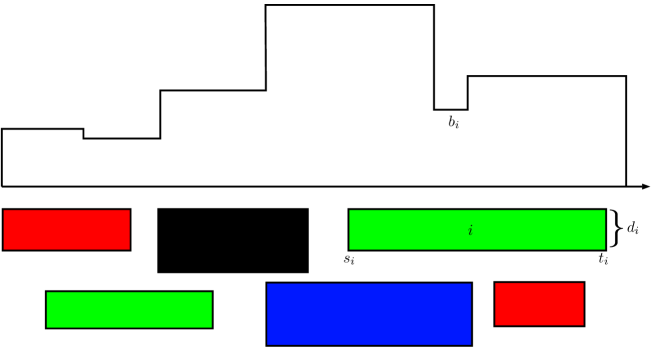
Figure 6.1: Illustration of the main concept of a bagUFP instance. Each task $i$ is represented as a rectangle, where the starting and ending $x$-coordinate represent $s_{i}$ and $t_{i}$, while the height represents the demand of that task; $b_{i}$ is the bottleneck capacity of task $i$. Tasks in the same bag are represented with the same color.

Lemma 82.

Suppose that there is an $\alpha$-approximation for the special case when all the tasks are small, and a $\beta$-approximation for the case when all the tasks are large, for some $\alpha,\beta\geq 1$. Then there exists a $\alpha+\beta$ approximation algorithm for the general case.

Proof.

Consider an instance of bagUFP with set of tasks $T$. Suppose that $T=T_{S}\mathbin{\dot{\cup}}T_{L}$, where $T_{S}$ and $T_{L}$ are the small and large tasks, respectively. Let $OPT$ be the optimal solution, and let $OPT_{S}=OPT\cap T_{S}$ and $OPT_{L}=OPT\cap T_{L}$.
We run the $\alpha$-approximation on $T_{S}$ the $\beta$-approximation on $T_{L}$ to obtain the feasible solutions $APX_{S}$ and $APX_{L}$, respectively; then we output the one with largest profit, let it be $APX$.
Clearly, $p(APX_{S})\geq p(OPT_{S})/\alpha$ and $p(APX_{L})\geq p(OPT_{L})/\beta$, which implies:

$$p(APX) =\max\left\{p(APX_{S}),p(APX_{L})\right\}\geq\frac{\alpha p(APX_{S})+\beta p(APX_{L})}{\alpha+\beta}$$

$$\geq\frac{p(OPT_{S})+p(OPT_{L})}{\alpha+\beta}=\frac{p(OPT)}{\alpha+\beta}$$

∎

Many results on this problem (and its variations) are indeed based on partitioning the items in the two classes of small and large, although the exact definition might be different from the one we use here. In fact, when items are relatively small, LP-based techniques have been applied successfully; but they would break down on large items. Vice versa, for relatively large items, good results are typically obtained with Dynamic Programming algorithms. Note that even if algorithms were found that solve exactly instances with either only small items or only large items, Lemmsa 82 only guarantees a $2$-approximation overall. Thus, breaking the barrier of $2$, if it is possible, would requires fundamentally new ideas that allow to handle small and large items simultaneously.

Using the primal-dual technique, for instances of bagUFP entirely composed of small tasks, Chakaravarthy et al. [2014] proved the following:

Lemma 83 (Chakaravarthy et al. [2014]).

There exists a $9$-approximation algorithm for the bagUFP problem running in time $O\left(n^{2}\right)$, if all the tasks are small.

Thus, in the following we can focus on instances where all tasks are large.

The natural linear programming relaxation for bagUFP, denoted by LP${}_{\textup{bagUFP}}$ is given below. The LP has a variable $x_{i}$ for each task $i\in T$.

maximize $$\textstyle\sum_{i:T_{i}\in\mathcal{T}}w_{i}x_{i} \left(\mbox{LP${}_{\textup{bagUFP}}$}\right)$$

s.t. $$\textstyle\sum_{i:e\in T_{i}}d_{i}x_{i}\leq u_{e} \forall e\in E$$

$$\textstyle\sum_{T_{i}\in\mathcal{B}_{j}}x_{i}\leq 1 \forall\mathcal{B}_{j}\in J$$

$$x_{i}\geq 0 \forall T_{i}\in\mathcal{T}$$

Note that, if the variables are restricted to $\{0,1\}$, this is the exact integer programming formulation of the problem.

As it was first done by Bonsma et al. [2011], for large tasks we exploit a connection to the Maximum Weight Independent Set of Rectangles (MWISR) problem, which is the following problem: given a set of axis-aligned rectangles in the plane, each with an associated weight, find the maximum weight set of pairwise non-overlapping rectangles. The best known polynomial time approximation for this problem is an $O(\log n/\log\log n)$-approximation by Chan and Har-Peled [2012], although Chalermsook and Chuzhoy [2009] gave a $O(\log\log n)$-approximation for the unweighted (cardinality) case. Moreover, a QPTAS was given in Adamaszek and Wiese [2013].

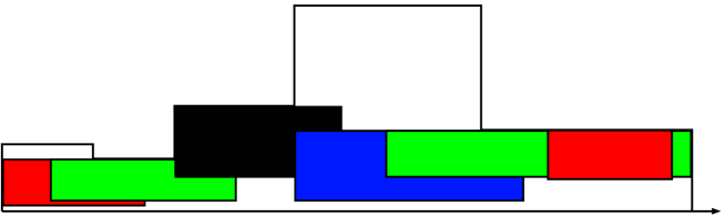
Figure 6.2: The top-drawn instance corresponding to the tasks in Figure 6.1.

For each large task $i$ of a UFP instance, we associate the rectangle $R_{i}$ with top-left corner $(s_{i},b_{i})$ and bottom-right corner $(t_{i},l_{i})$ where $l_{i}=b_{i}-d_{i}$. We call this set of rectangles the top-drawn instance corresponding to $T_{\textup{large}}$ (see Figure 6.2 for an illustration of the capacity profile and a top-drawn instance). Thus, the set of rectangles $\mathcal{R}=\left\{R_{i}\right\}_{i}$ with the weight function $w_{i}$ defines an MWISR instance, and it is easy to see that a feasible solution for the MWISR instance corresponds to a feasible subset of task in the UFP instance. Moreover the following result applies:

Lemma 84 (implied by Lemma 13 in Bonsma et al. [2011]).

Suppose that all tasks are large. Then any feasible UFP solution $S$ can be partitioned in $4$ sets $S_{1},\dots,S_{4}$ such that each $S_{j}$ is an independent set of rectangles.

A similar reduction works for bagUFP, except that what we obtain is an instance of the natural generalization of the MWISR problem that we call bagMWISR, where we also preserve the bag constraints between rectangles, corresponding to the original bag constraints among tasks.

We define the set $\mathcal{P}$ as follows. We consider the (non-uniform) grid induced by the horizontal and vertical lines containing the edges of the rectangles. For each finite cell in this grid, we add its center to $\mathcal{P}$ if and only if it overlaps with at least one rectangle in $\mathcal{R}$, as shown in Figure 6.3. Clearly, $|\mathcal{P}|=O(n^{2})$, since the grid is defined by at most $2n$ horizontal and at most $2n$ vertical lines.

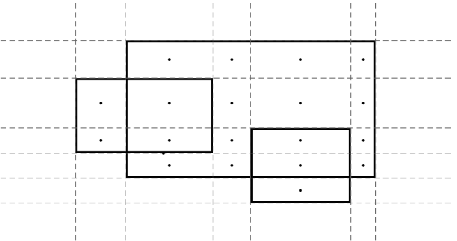
Figure 6.3: The points in $\mathcal{P}$ in the definition of LP${}_{\textup{bagMWISR}}$.

The following is the natural LP relaxation for the bagMWISR problem, which we denote by LP${}_{\textup{bagMWISR}}$. There is a variable $y_{i}$ for each rectangle $R_{i}\in\mathcal{R}$, and we define $\mathcal{P}$ as the set of corners of rectangles in $\mathcal{R}$, plus each intersection point of a vertical edge of $R_{i}$ and a horizontal edge of $R_{j}$, for any two rectangles $R_{i},R_{j}\in\mathcal{R}$.

maximize $$\textstyle\sum_{R_{i}\in\mathcal{R}}w_{i}y_{i} \left(\mbox{LP${}_{\textup{bagMWISR}}$}\right)$$

s.t. $$\textstyle\sum_{R_{i}\in\mathcal{R}:p\in R_{i}}y_{i}\leq 1 \forall\,p\in\mathcal{P}$$

$$\textstyle\sum_{R_{i}\in\mathcal{B}_{j}}y_{i}\leq 1 \forall\,\mathcal{B}_{j}\in J$$

$$y_{i}\geq 0 \forall\,R_{i}\in\mathcal{R}$$

Let $\mathbf{y}$ be the optimal solution and let $opt=\sum_{R_{i}\in\mathcal{R}}w_{i}y_{i}$ be its value. Clearly, if $OPT$ is the value of the optimal integral solution, $opt\geq OPT$.

In the next two sections, we describe approximation algorithms for bagMWISR and, as a corollary, improved approximations for bagUFP. These results have been published in Grandoni, Ingala and Uniyal [2015]. In the same paper, we also considered a special case of bagUFP, that we call UFP with time windows (twUFP). Here, together with the path graph $G$, we are given a collection of jobs. Each job $j$ is characterized by a weight, a demand $\tau_{j}$, and a time window, which is the sub-path between two given nodes $s_{j}$ and $t_{j}$. For each possible node $\delta_{i}$ such that $s_{j}\leq\delta_{i}\leq t_{j}-\tau_{j}$, we define a task $i$ with the same weight and demand as $i$, and whose subpath $P_{i}$ has the starting point $s_{i}=\delta_{i}$ and the endpoint $t_{i}=s_{i}+\tau_{j}$. The tasks corresponding to the same job $j$ define a bag $\mathcal{B}_{j}$.

We introduce a limitation to the instances of twUFP that we call Bounded Time-Window Assumption (BTWA): namely, we assume that there exists a fixed positive constant $C$ such that $t_{j}-s_{j}\leq Ct_{j}$ for each job $j$; that is, the time window size is bigger than the processing time by at most a constant factor. We proved the following result:

Theorem 85.

There is a QPTAS for twUFP under BTWA and assuming that demands are quasi-polynomially bounded in $n$.

This result is a generalization of the QPTAS for UFP by Bansal, Chakrabarti, Epstein and Schieber [2006].

6.3 A $O(\log n/\log\log n)$-approximation for bagUFP

In this section, we show how to extend the analysis in Chan and Har-Peled [2012] for MWISR to bagMWISR, obtaining an expected $O\left(\log n/\log\log n\right)$-approximation.

First, we consider the general case. We say that two rectangles cross if they overlap but no rectangle contains a vertex of the other rectangle. Construct two undirected graphs $G_{1}$ and $G_{2}$ with vertex set $\mathcal{R}$ such the edge $(R_{i},R_{j})$ is in $G_{1}$ if the rectangles $R_{i}$ and $R_{j}$ are in the same bag, or if they overlap but do not cross; and $(R_{i},R_{j})$ is in $G_{2}$ if they cross. Clearly, a set $S\subseteq\mathcal{R}$ is an independent set of rectangles which satisfies the bag constraints if and only if it is an independent set in both $G_{1}$ and $G_{2}$. We have the following lemma:

Lemma 86.

Suppose that a set $S\subseteq\mathcal{R}$ is an independent set in $G_{1}$; moreover, suppose that the induced subgraph $G_{2}[S]$ has maximum clique size $\Delta$. Then it is possible to color in polynomial time each rectangle in $S$ using at most $\Delta$ colors so that no edge of $G_{2}[S]$ connects two rectangles of the same color.

Proof.

Call a rectangle $R_{i}$ thinnest if no rectangle crosses $R_{i}$ and has a smaller width. Let $S_{1}$ be the set of thinnest rectangles. Clearly, they are pairwise not crossing and hence not overlapping, and thus they form an independent set (see Figure 6.4). We assign a color to the rectangles in $S_{1}$ and we remove them from the graph (together with the incident edges); clearly, the residual graph has maximum clique size at most $\Delta-1$, and so we can iterate the process to obtain the independent sets $S_{1},S_{2},\dots,S_{\Delta}$. ∎

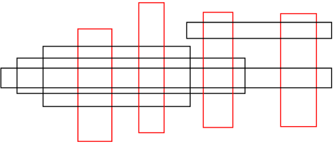
Figure 6.4: Proof of Lemma 86. The thinnest rectangles (in red) are independent, and removing them decreases the maximum clique size.

Consequently, if we find a set $S$ such that $G_{1}[S]$ is an independent set and $G_{2}[S]$ has maximum clique size $\Delta$, then we can find an independent set of rectangles $S^{\prime}$ of profit at least $p(S)/\Delta$. We will find such a set $S$ with the technique of randomized rounding of the LP solution.

6.3.1 Algorithm

For two rectangles $R_{i}$ and $R_{j}$, we write that $R_{i}\otimes R_{j}$ if the interior of $R_{i}$ contains at least one corner of $R_{j}$, or vice versa; that is, $R_{i}\otimes R_{j}$ if $R_{i}$ and $R_{j}$ overlap but do not cross.

For an arbitrary set $\mathcal{K}\subseteq\mathcal{R}$ and rectangle $R_{i}\in\mathcal{R}$, we define the resistance $\eta$ as:

$$\eta(R_{i},\mathcal{K})=\sum_{\begin{subarray}{c}R_{j}\in\mathcal{K}\setminus\mathcal{B}(R_{i}),\\ R_{i}\otimes R_{j}\end{subarray}}y_{j}+\sum_{R_{j}\in\mathcal{K}\cap\mathcal{B}(R_{i})\setminus\{R_{i}\}}y_{j}$$

That is, $\eta(R_{i},\mathcal{K})$ is the sum of each $y_{j}$ for some $R_{j}\in\mathcal{K}$ such that $R_{i}\otimes R_{j}$, or $R_{i}$ and $R_{j}$ are in the same bag.

The algorithm works as follows. First, a fractional optimal solution $\mathbf{y}$ of LP${}_{\textup{bagMWISR}}$ is computed. Then a permutation $\Pi$ of $\mathcal{R}$ is obtained as follows: if the first $i$ elements are $\Pi_{i}=\{\pi_{1},\dots,\pi_{i}\}$, then the $(i+1)^{th}$ element $\pi_{i+1}$ is:

$$\pi_{i+1}=\arg\min_{R_{j}\in\mathcal{R}\setminus\Pi_{i}}{\eta(R_{j},\mathcal{R}\setminus\Pi_{i})}$$

Let $\eta_{i}=\eta(\pi_{i},\mathcal{R}\setminus\Pi_{i-1})$ be the resistance of the $i^{th}$ rectangle. After the permutation is computed, a candidate set $C$ and an independent set $S$ for $G_{1}$ are computed with the following process. Initially, $C$ and $S$ are empty. Then, the members of the permutation are scanned in reverse order: at iteration $k$, the rectangle $\pi_{m-(k-1)}$ is added to set $C$ (initially empty) with probability $y(\pi_{m-(k-1)})/\tau$, where $\tau>1$ is a constant integer parameter that will be defined later. If $\pi_{m-(k-1)}$ is added to $C$ and $S\cup\{\pi_{m-(k-1)}\}$ is an independent set in $G_{1}$, then $\pi_{m-(k-1)}$ is also added to $S$.

Finally, by using Lemma 86, the algorithm finds a subset $S^{\prime}\subseteq S$ that is an independent set in $G_{2}[S]$ such that $p(S^{\prime})\geq p(S)/\Delta$, where $\Delta$ is the maximum clique size of $G_{2}[S]$.

6.3.2 Analysis

For a subset $\mathcal{H}\subseteq\mathcal{R}$, let us define $\mathcal{E}(\mathcal{H})=\sum_{R_{i}\in\mathcal{H}}y_{i}$; moreover, let $\mathcal{C}(\mathcal{H})=\{(p,i,j)\;|\;p\mbox{ is a corner of }R_{i},\mbox{ where }R_{i},R_{j}\in\mathcal{R},i\neq j,p\in R_{j}\}$.

Lemma 87.

Let $\mathcal{H}$ be any subset of $\mathcal{R}$. Then $\sum_{(p,i,j)\in\mathcal{C}(\mathcal{H})}y_{i}y_{j}\leq 4\mathcal{E}(\mathcal{H})$.

Proof.

$\displaystyle\sum_{(p,i,j)\in\mathcal{C}(\mathcal{H})}y_{i}y_{j}=\sum_{i\in\mathcal{H}}y_{i}\sum_{j:(p,i,j)\in\mathcal{C}(\mathcal{H})}y_{j}\leq 4\sum_{i\in\mathcal{H}}y_{i}=4\mathcal{E}(\mathcal{H})$.
The inequality follows from the feasibility of $\mathbf{y}$ and the fact that there are four corner points for each rectangle. ∎

Lemma 88.

For any $i$, the resistance of the $i^{th}$ chosen rectangle $\pi_{i}$ is at most $5$.

Proof.

Fix an $i$, and let $\mathcal{K}=\mathcal{R}\setminus\left\{\pi_{1},\dots,\pi_{i-1}\right\}$. We have

$$\sum_{R_{k}\in\mathcal{K}}y_{k}\eta(R_{k},\mathcal{K}) =\sum_{R_{k}\in\mathcal{K}}y_{k}\sum_{\begin{subarray}{c}R_{j}\in\mathcal{K}\setminus\mathcal{B}(R_{k}),\\ R_{k}\otimes R_{j}\end{subarray}}y_{j}+\sum_{R_{k}\in\mathcal{K}}y_{k}\sum_{R_{j}\in\mathcal{K}\cap\mathcal{B}(R_{k})\setminus\{R_{k}\}}y_{j}$$

$$\leq\sum_{R_{k}\in\mathcal{K}}y_{k}\sum_{\begin{subarray}{c}R_{j}\in\mathcal{K},\\ R_{k}\otimes R_{j}\end{subarray}}y_{j}+\sum_{R_{k}\in\mathcal{K}}y_{k}\sum_{R_{j}\in\mathcal{B}(R_{k})}y_{j}$$

We first prove:

$$\sum_{R_{k}\in\mathcal{K}}y_{k}\sum_{\begin{subarray}{c}R_{j}\in\mathcal{K},\\ R_{k}\otimes R_{j}\end{subarray}}y_{j}\leq\sum_{(p,i,j)\in\mathcal{C}(\mathcal{K})}y_{i}y_{j}$$

Then, by Lemma 87, the right hand side is at most $4\mathcal{E}(\mathcal{H})$. Note that, for each pair of distinct rectangles $R_{i},R_{j}\in\mathcal{K}$ such that $R_{i}\otimes R_{j}$, the term $y_{i}y_{j}$ appears in the left hand side exactly twice. Now we prove the above inequality by showing that the term $y_{i}y_{j}$ appears at least twice in the right hand side. If we fix any pair $R_{i},R_{j}\in\mathcal{K}$, there are three cases (see Figure 6.5):

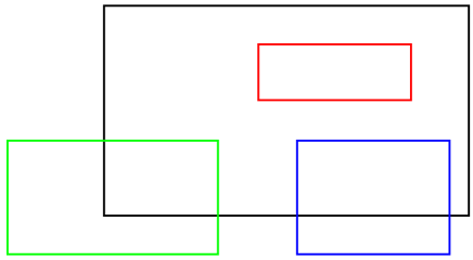
Figure 6.5: Three types of rectangles that overlap with the black rectangle, without creating a crossing intersection. The black rectangle contains all the 4 corners of the red rectangles, and exactly two corners of the blue rectangle. The green rectangle contains one corner of the black rectangle which, in turn, contains one corner of the green rerctangle.

1. one rectangle, say $R_{i}$, contains all the 4 corners of the other: then the term $y_{i}y_{j}$ appears four times in the right hand side.

2. one rectangle, say $R_{i}$, contains exactly 2 corners of the other: then the term $y_{i}y_{j}$ appears twice in the right hand side.

3. each rectangle contains exactly one corner of the other: then again the term $y_{i}y_{j}$ appears twice in the right hand side.

Moreover, because of the constraints of bagMWISR, it follows that:

$$\sum_{R_{k}\in\mathcal{K}}y_{k}\sum_{R_{j}\in\mathcal{B}(R_{k})}y_{j}\leq\sum_{R_{k}\in\mathcal{K}}y_{k}=\mathcal{E}(\mathcal{K})$$

Thus, we have proved:

$$\sum_{R_{k}\in\mathcal{K}}y_{k}\eta(R_{k},\mathcal{K}) \leq 4\mathcal{E}(\mathcal{K})+\mathcal{E}(\mathcal{K})=5\mathcal{E}(\mathcal{K})$$

$$\Longrightarrow\sum_{R_{k}\in\mathcal{K}}\frac{y_{j}}{\mathcal{E}(\mathcal{K})}\eta(R_{k},\mathcal{K})\leq 5.$$

Since the left hand side of the last inequality is a convex combination of the elements of the set $\left\{\eta(R_{k},\mathcal{K})\enspace|\enspace R_{k}\in\mathcal{K}\right\}$, it follows that $\displaystyle{\min_{R_{k}\,\in\mathcal{K}}\{\eta(R_{k},\mathcal{K})\}\leq 5}$. This concludes the proof, because the algorithm always chooses the rectangle that minimizes the resistance. ∎

Lemma 89.

Setting $\tau=10$, then $\operatorname*{\mathbb{E}}[w(S)]\geq Opt/20$.

Proof.

Let $j^{\prime}=\pi(j)$. Observe that the $R_{j^{\prime}}$, is added to the candidate set $C$ with probability $x_{j^{\prime}}/\tau$. Let $\mathcal{K}$ be the set of rectangles $R_{i}$ that were already considered and such that $R_{j^{\prime}}\otimes R_{i}$ or $R_{i}$ is in the same bag as $R_{j^{\prime}}$. Clearly, $\mathcal{E}(\mathcal{K})$ equals the resistance $\eta_{j}$ of $R_{j^{\prime}}$ in the moment it is added to the permutation. Thus:

$$\Pr[R_{j^{\prime}}\in I\,|\,R_{j^{\prime}}\in C]=\prod_{R_{i}\in\mathcal{K}}\left(1-\frac{y_{i}}{\tau}\right)\geq 1-\sum_{R_{i}\in\mathcal{K}}\frac{y_{i}}{\tau}=1-\frac{\mathcal{E}(\mathcal{K})}{\tau}\geq\frac{1}{2}$$

because of Lemma 88. Thus, we have:

$$\Pr[R_{j^{\prime}}\in I]=\Pr[R_{j^{\prime}}\in S\,|\,R_{j^{\prime}}\in C]\cdot\Pr[R_{j^{\prime}}\in C]\geq\frac{y_{j^{\prime}}}{2\tau}$$

Thus, we have:

$$\operatorname*{\mathbb{E}}[S^{\prime}]=\sum_{\Pr[R_{j^{\prime}}\in I]}w_{j^{\prime}}\geq\sum_{\Pr[R_{j^{\prime}}\in I]}\frac{y_{j^{\prime}}w_{j^{\prime}}}{2\tau}=\frac{Opt}{20}$$

∎

Lemma 90.

With probability at least $1-1/n$, the maximum depth of the rectangles in $I$ is $\displaystyle\Delta=O\left(\frac{\log n}{\log\log n}\right)$.

Proof.

Fix a point $p\in\mathcal{P}$. The number $\operatorname{depth}(p,I)$ of rectangles in $I$ containing $p$ is a sum of independent 0–1 random variables with mean $\mu=\sum_{R_{i}\ni p}\frac{y_{u}}{\tau}\leq 1$. Thus, by Chernoff bound:

$$\Pr[\operatorname{depth}(p,I)>(1+\delta)\mu]<{\left(\frac{e^{\delta}}{{(1+\delta)}^{1+\delta}}\right)}^{\mu}$$

for any $\delta>0$. By choosing $\delta$ such that $t=(1+\delta)\mu$, it holds that:

$$\Pr[\operatorname{depth}(p,I)>t]<{(e/t)}^{t}$$

Since $|\mathcal{P}|=O(n^{2})$ and $\Delta=\max_{p\in\mathcal{P}}\operatorname{depth}(p,I)$, by the union bound it follows that $\Pr[\Delta>t]=O({(e/t)}^{t}n^{2})$, which is at most $1/n$ for $t=\Theta(\log n/\log\log n)$. ∎

Lemma 91.

There is an expected $O\left(\dfrac{\log n}{\log\log n}\right)$-approximation for bagMWISR.

Proof.

Clearly, we have that $\sum_{R_{i}\in S^{\prime}}w_{i}\geq\frac{1}{\Delta}\sum_{R_{i}\in S}w_{i}$. Thus:

$$E\left[\sum_{R_{i}\in S^{\prime}}w_{i}\right] \geq\left(1-\frac{1}{n}\right)\Omega\left(\frac{\log\log n}{\log n}\right)E\left[\sum_{R_{i}\in S}w_{i}\right] \geq\Omega\left(\frac{\log\log n}{\log n}\right)Opt$$

∎

We finally obtain the following:

Theorem 92.

There is an expected $O\left(\dfrac{\log n}{\log\log n}\right)$-approximation for bagUFP.

Proof.

The result follows immediately by combining Lemmas 82, 83 and 91. ∎

6.4 A $O(1)$-approximation for the unweighted case

In this section we present a $O(1)$-approximation for bagUFP with large tasks, assuming uniform profits. This analysis extends the framework of Anagnostopoulos et al. [2013], which only considered the UFP problem without handling bag constraints.

For any horizontal coordinate $x\in[0,m)$, we define for simplicity:

$$c(x):=c_{(\left\lfloor x\right\rfloor,\left\lfloor x\right\rfloor+1)}.$$

We start with an arbitrary maximal feasible set of rectangles $\mathcal{R}_{\textup{M}}\subseteq\mathcal{R}$.

Let $\mathcal{R}_{\textup{bag}}$ be the set of all rectangles in $\mathcal{R}$ that belongs to some bag $J\ni R_{i}$ for each $R_{i}\in\mathcal{R}_{\textup{M}}$. Notice that $\mathcal{R}_{\textup{bag}}\supseteq\mathcal{R}_{\textup{M}}$.

Lemma 93.

We have that $\displaystyle\sum_{R_{j}\in\mathcal{R}_{\textup{bag}}}y_{j}\leq|\mathcal{R}_{\textup{M}}|$.

Proof.

Consider the bag $\mathcal{B}_{j}$ of a rectangle $R_{i}\in\mathcal{R}_{\textup{M}}$. From the LP${}_{\textup{bagMIWSR}}$ constraint for $\mathcal{B}_{j}$, we have: $\sum_{R_{j}\in\mathcal{B}_{j}}y_{j}\leq 1$, Since, $\mathcal{R}_{\textup{M}}$ is a feasible solution of bagUFP problem, so each $R_{i}\in\mathcal{R}_{\textup{M}}$ will belong to a distinct bag. Therefore, if we sum over all bags $\mathcal{B}_{j}$ such that $\mathcal{B}_{j}\ni R_{i}:R_{i}\in\mathcal{R}_{\textup{M}}$, we get the inequality:

$$\sum_{R_{j}\in\mathcal{R}_{\textup{bag}}}y_{j}=\sum_{{\mathcal{B}_{j}\ni R_{i}:R_{i}\in\mathcal{R}_{\textup{M}}}}\sum_{R_{j}\in\mathcal{B}_{j}}y_{j}\leq|\mathcal{R}_{\textup{M}}|.$$

∎

Let $\mathcal{Q}_{\textup{corner}}$ be the set of corner points of all the rectangles in $\mathcal{R}_{\textup{M}}$. Let $\mathcal{R}_{\textup{corner}}$ be the set of all rectangles in $\mathcal{R}\setminus\mathcal{R}_{\textup{bag}}$ that intersects with at least one of the points in $\mathcal{Q}_{\textup{corner}}$.

Lemma 94.

We have that $\sum_{R_{j}\in\mathcal{R}_{\textup{corner}}}y_{j}\leq 4|\mathcal{R}_{\textup{M}}|$.

Proof.

Consider the top-left corner $p_{i}=(s_{i},b_{i})\in\mathcal{P}$ of a rectangle $R_{i}\in\mathcal{R}_{\textup{M}}$. Then $\sum_{{R_{i}\in\mathcal{R}_{\textup{corner}}:p_{i}\in R_{j}}}y_{j}\leq\sum_{{R_{j}\in\mathcal{R}:p_{i}\in R_{j}}}y_{j}\leq 1$, by LP${}_{\textup{bagMWISR}}$ constraints. Hence if $\mathcal{R}_{\textup{TL}}$ is the set of all the rectangles in $\mathcal{R}_{\textup{corner}}$ that contain the top-left corner of some rectangle in $\mathcal{R}_{\textup{M}}$, we have:

$$\sum_{R_{j}\in\mathcal{R}_{\textup{TL}}}y_{j}\leq\sum_{R_{i}\in\mathcal{R}_{\textup{M}}}\sum_{\begin{subarray}{c}R_{j}\in\mathcal{R}_{\textup{corner}}:\\ p_{i}\in R_{j}\end{subarray}}y_{j}\leq\sum_{R_{i}\in\mathcal{R}_{\textup{M}}}1\leq|\mathcal{R}_{\textup{M}}|.$$

The result follows by summing up this inequality with the analogous one for the top-right, bottom-left and bottom-right corners. ∎

Let $\mathcal{R}^{\prime}=(\mathcal{R}\setminus\mathcal{R}_{\textup{M}})\setminus(\mathcal{R}_{\textup{bag}}\cup\mathcal{R}_{\textrm{corner}})$. Note that each rectangle $R_{j}\in\mathcal{R}^{\prime}$ overlaps with some rectangle in $\mathcal{R}_{\textup{M}}$. As illustrated in Figure 6.6, we now classify the rectangles in $\mathcal{R}^{\prime}$ into three groups (not necessarily disjoint) as follows:

1. Top-intersecting ($\mathcal{R}_{\textup{T}}$): We call a rectangle $R_{j}\in\mathcal{R}^{\prime}$ top-intersecting if there exists a rectangle $R_{i}\in\mathcal{R}_{\textup{M}}$ such that $s_{i}<s_{j}<t_{j}<t_{i}$ and $b_{j}\geq b_{i}>l_{j}$.

2. Left-intersecting ($\mathcal{R}_{\textup{L}}$): We call a rectangle $R_{j}\in\mathcal{R}^{\prime}$ left-intersecting if there exists a rectangle $R_{i}\in\mathcal{R}_{\textup{M}}$ such that $b_{i}>b_{j}>l_{j}>l_{i}$ ; $s_{j}<s_{i}<t_{j}$ and $\exists x_{B}\in[s_{j},s_{i}]$ such that $c(x_{B})=b_{j}$.

3. Right-intersecting ($\mathcal{R}_{\textup{R}}$): We call a rectangle $R_{j}\in\mathcal{R}^{\prime}$ right-intersecting if there exists a rectangle $R_{i}\in\mathcal{R}_{\textup{M}}$ such that $b_{i}>b_{j}>l_{j}>l_{i}$ ; $s_{j}<t_{i}<t_{j}$ and $\exists x_{B}\in[t_{i},t_{j}]$ such that $c(x_{B})=b_{j}$.

From now on we call a rectangle $R_{j}\in\mathcal{R}^{\prime}$ to be top (left, right, resp.) intersecting to a rectangle $R_{i}\in\mathcal{R}_{\textup{M}}$ if it satisfies the conditions in 1. (2., 3., resp.).

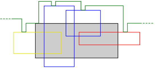
Figure 6.6: The black rectangle with gray background is in $\mathcal{R}_{\textup{M}}$. The blue ones are top-intersecting; the yellow one is left-intersecting; the red one is right-intersecting. Note that a rectangle could simultaneously be left-intersecting to a rectangle and right-intersecting to another one.

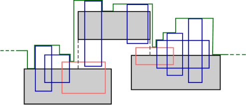
Figure 6.7: Illustration of some of the concepts for the $O(1)$-approximation for unweighted bagUFP. The green curve is the capacity profile, and the rectangles are part of a top-drawn instance of bagUFP. Black rectangles with gray background are in the initial maximal feasible solution $\mathcal{R}_{\textup{M}}$, while all the other rectangles are in $\mathcal{R}_{\textup{T}}$ (for simplicity, in this picture there are no rectangles in $\mathcal{R}_{\textup{bag}}$ and $\mathcal{R}_{\textup{corner}}$, as well as in $\mathcal{R}_{\textup{L}}$ and $\mathcal{R}_{\textup{R}}$). Red rectangles are in $\mathcal{R}^{\textup{point}}_{\textup{top}}$, while the remaining blue rectangles are in $\mathcal{R}_{top}$.

Proposition 95.

All the rectangles in $\mathcal{R}^{\prime}$ are either top-intersecting, left-intersecting, or right-intersecting.

In order to bound the profit of rectangles in $\mathcal{R}_{\textup{T}}$, we divide it into two sets. First we define a set of points $\mathcal{Q}_{\textup{T}}$ created according to the following process. For each bottom corner of each rectangle in $\mathcal{R}_{\textup{M}}$, we project vertically downwards until we meet another rectangle in $\mathcal{R}_{\textup{M}}$ or we arrive at height 0. More formally, we define $\mathcal{Q}_{\textup{T}}$ as the set of points $(x,y)$ for which there exist two rectangles $R_{i},R_{j}\in\mathcal{R}_{\textup{M}}$ such that the following conditions hold:

1. $l_{i}>b_{j}$

2. $x\in\{s_{i},t_{i}\}$, and $s_{j}<x<t_{j}$

3. $y=b_{j}$

4. $\not\exists\,R_{k}\in\mathcal{R}_{\textup{M}}$ such that $s^{\prime}_{k}<x<t_{k}$ and $l_{i}<b_{k}<b_{j}\}$

Let $\mathcal{R}^{\textup{point}}_{\textup{top}}$ be the subset of rectangles in $\mathcal{R}_{\textup{T}}$ containing at least one point in $\mathcal{Q}_{\textup{T}}$, and let $\mathcal{R}_{\textup{top}}=\mathcal{R}_{\textup{T}}\setminus\mathcal{R}^{\textup{point}}_{\textup{top}}$. We now bound the total contribution of $\mathcal{R}^{\textup{point}}_{\textup{top}}$ to the profit of the LP solution.

Lemma 96.

We have that $\sum_{R_{i}\in\mathcal{R}^{\textup{point}}_{\textup{top}}}y_{i}\leq 2|\mathcal{R}_{\textup{M}}|$.

Proof.

Note that for any $R_{j}\in\mathcal{R}_{\textup{M}}$, there are at most two points in $\mathcal{Q}_{\textup{T}}$ corresponding to the projection of the bottom corner points ${(s_{j},l_{j}),(t_{j},l_{j})}$.The result follow by a similar argument as in the proof of Lemma 94. ∎

Next we show that the bagMWISR for $\mathcal{R}_{\textup{top}}$ can be reduced to an independent set of intervals problem with bag constraints.

Lemma 97.

Two rectangles $R_{i},R_{j}\in\mathcal{R}_{\textup{top}}$ overlap if and only if $[s_{i},t_{i}]\cap[s_{j},t_{j}]\neq\phi$.

Proof.

If $[s_{i},t_{i}]\cap[s_{j},t_{j}]=\phi$, then the two rectangles do not overlap.

Assume by contradiction that $[s_{i},t_{i}]\cap[s_{j},t_{j}]\neq\phi$, but the two rectangles do not overlap. Without loss of generality, assume that $R_{i}$ is above $R_{j}$ (that is, $l_{i}\geq b_{j}$). Since it is a top-drawn instance, $s_{j}<x<t_{j}$ for some $x\in\{s_{i},t_{i}\}$. Let $R_{\overline{i}}$ (resp. $R_{\overline{j}}$) be a rectangle in $\mathcal{R}_{\textup{M}}$ to which $R_{i}$ (resp. $R_{j}$) is top-intersecting. Since $s_{\overline{i}}<s_{i}<t_{i}<t_{\overline{i}}$, then $l_{\overline{i}}>b_{j}$ (otherwise $R_{j}$ would be in $\mathcal{R}_{\textup{corner}}$). Consider the following algorithm. The algorithm keeps track of a rectangle $R$ with the following properties:

• $R\in\mathcal{R}_{\textup{M}}$;

• the coordinates of one of the two bottom corners of $R$, say $(x_{R},y_{R})$, satisfy $s_{j}<x_{R}<t_{j}$ and $y_{R}>b_{j}$.

The algorithm starts by setting $R\leftarrow R_{\overline{i}}$, which satisfies all the conditions above; at each step, the algorithm chooses a bottom corner of $R$, say $(x_{R},y_{R})$, such that $s_{j}<x_{R}<t_{j}$. Then it finds the point $P=(x_{P},y_{P})$ obtained by moving vertically downward starting from $(x_{R},y_{R})$ till it meets the top edge of some rectangle $R^{\prime}\in\mathcal{R}_{\textup{M}}$ (it may be that $R^{\prime}=R_{\overline{j}}$). Let the bottom left and top right corners of $R^{\prime}$ be $(s_{R^{\prime}},l_{R^{\prime}})$ and $(t_{R^{\prime}},b_{R^{\prime}})$, respectively. Note that since the instance is top-drawn, one of the coordinates $x\in\{s_{R^{\prime}},t_{R^{\prime}}\}$ will be in the range $\left(s_{j},t_{j}\right)$, if $R^{\prime}\neq R_{\overline{j}}$. There are three cases:

• $y_{P}\leq b_{j}$: then $P\in R_{j}$, implying $R_{j}\in\mathcal{R}^{\textup{point}}_{\textup{top}}$, which is a contradiction;

• $y_{P}>b_{j}$ and $l_{R^{\prime}}\leq b_{j}$: then for some $x\in\{s_{R^{\prime}},t_{R^{\prime}}\}$ the corner $(x,l_{R^{\prime}})$ of $R^{\prime}$ is contained in $R_{j}$ and so $R_{j}\in\mathcal{R}_{\textup{corner}}$, which is a contradiction;

• $y_{P}>b_{j}$ and $l_{R^{\prime}}>b_{j}$: then $R^{\prime}$ satisfies the above conditions, and the algorithm continues by setting $R\leftarrow R^{\prime}$ and going to the next step.

Note that the $y$-coordinate of the top edge of $R$ is strictly smaller at each iteration, so a contradiction must eventually be found. ∎

Thus, the problem of finding a maximum set of independent rectangles in $\mathcal{R}_{\textup{top}}$ with bag constraints is equivalent to solving the corresponding instance of the maximum set of independent intervals problem with bag constraints. There is a $2$-approximation algorithm for this problem, see for example Bar-Noy, Guha, Naor and Schieber [2001] or Berman and DasGupta [2000].

Similarly we need to bound the contribution of the left-intersecting rectangles ($\mathcal{R}_{\textup{L}}$) to the profit of the LP solution. For this we need to define a set of points $\mathcal{Q}_{L}$ (as we did with the set of points $\mathcal{Q}_{\textup{T}}$). First we define the mapping from one point to another as:

$$f(x,y)=\left\{\begin{array}[]{l l}\text{min${}_{s_{i}}$ $(s_{i},y)$}&\enskip\text{if $\exists R_{i}\in\mathcal{R}_{\textup{M}}$: $s_{i}\geq x$ and $l_{i}\leq y\leq b_{i}$}\\ &\text{ and $c(x^{\prime})\geq y$ for all $x<x^{\prime}\leq s_{i}$,}\\ \text{min${}_{x^{\prime}}$ $f(x^{\prime},c(x^{\prime}))$}&\enskip\text{if no such $R_{i}$ exists and if $\exists x^{\prime}>x$:}\\ &\text{$c(x^{\prime})<y$ and $c(x^{\prime\prime})\geq y$ for all $x<x^{\prime\prime}<x^{\prime}$}\\ \bot&\enskip\text{otherwise}\end{array}\right.$$

We now define the set $\mathcal{Q}_{L}=\{f(t_{i},b_{i})\,|\,R_{i}\in\mathcal{R}_{\textup{M}}\}$. Intuitively, for each rectangle in $\mathcal{R}_{\textup{M}}$ we start from the top-right corner and we move rightwards, stopping if we meet the left edge of any rectangle in $\mathcal{R}_{\textup{M}}$; if we meet a vertical edge of the capacity profile, we move downwards until it is possible to move rightwards again, and we continue the process (see Figure 6.8).

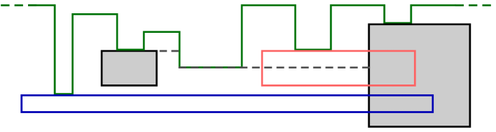
Figure 6.8: The definition of the set $\mathcal{R}_{left}^{point}$. The rectangles with gray background are in $\mathcal{R}_{\textup{M}}$; the colored rectangle are left-intersecting rectangle, but the red one is in $\mathcal{R}_{left}^{point}$ and the blue one is not.

As for the case of top-intersecting rectangles, we let $\mathcal{R}_{left}^{point}$ be the set of rectangles in $\mathcal{R}_{L}$ containing some point in $\mathcal{Q}_{L}$. In the next lemma we bound the contribution of rectangles in $\mathcal{R}_{left}^{point}$ to the LP${}_{\textup{bagMWISR}}$ solution profit.

Lemma 98.

We have that $\sum_{R_{i}\in\mathcal{R}^{\textup{point}}_{\textup{left}}}y_{i}\leq|\mathcal{R}_{\textup{M}}|$.

Proof.

Note that for any rectangle $R_{j}\in\mathcal{R}_{\textup{M}}$, there is at most one point in $\mathcal{Q}_{\textup{L}}$, which is the point we obtain by applying function $f$ to its top-right corner point. The result follows by a similar argument as in the proof of Lemma 94. ∎

Once again, we can reduce the bagMWISR problem for $\mathcal{R}_{\textup{left}}=\mathcal{R}_{L}\setminus\mathcal{R}^{\textup{point}}_{\textup{left}}$ to the maximum independent set of intervals problem with bag constraints.

Let $u_{MAX}:=\max_{e\in E}{u_{e}}$ be the maximum capacity.

We map each rectangle $R_{i}\in\mathcal{R}_{\textup{left}}$ to the interval $[u_{MAX}\cdot j+l_{i},u_{MAX}\cdot j+b_{i}]$, where $j$ is defined by: $s_{j}=\min_{R_{M}\in\mathcal{R}_{\textup{M}}}\{s_{M}:R_{i}\mbox{ is left-intersecting to }R_{M}\}$; that is, $R_{j}$ is the leftmost starting rectangle in $\mathcal{R}_{M}$ to which $R_{i}$ is left-intersecting.

Lemma 99.

Let $R_{i},R_{i^{\prime}}\in\mathcal{R}_{\textup{left}}$. Then $R_{i}$ and $R_{i^{\prime}}$ overlap if and only if the segments they are mapped to overlap.

Proof.

Let $R_{M}$ (resp. $R_{M^{\prime}})$ be the left-most starting rectangle in $\mathcal{R}_{\textup{M}}$ such that $R_{i}$ is left-intersecting to $R_{M}$ (resp. $R_{i^{\prime}}$ is left-intersecting to $R_{M^{\prime}}$). By the above definition of the mapping, $R_{i}$ is mapped to $[u_{MAX}\cdot M+l_{i},u_{MAX}\cdot M+b_{i}]$ and $R_{i^{\prime}}$ is mapped to $[u_{MAX}\cdot M^{\prime}+l_{i^{\prime}},u_{MAX}\cdot M^{\prime}+b_{i^{\prime}}]$.
If the intervals $[l_{i},b_{i}]$ and $[l_{i^{\prime}},b_{i^{\prime}}]$ do not overlap, then trivially $R_{i}$ and $R_{i^{\prime}}$ do not overlap and there is nothing else to prove. Suppose that the above intervals overlap: we will prove that the rectangles $R_{i}$ and $R_{i^{\prime}}$ overlap if and only if $R_{M}=R_{M^{\prime}}$.

• Suppose that $R_{M}=R_{M^{\prime}}$. Then, $M=M^{\prime}$ and the maps of the two intervals overlap, since $[l_{i},b_{i}]$ and $[l_{i^{\prime}},b_{i^{\prime}}]$ overlap.

• Suppose that $R_{i}$ and $R_{i^{\prime}}$ overlap. We will prove that $R_{M}=R_{M^{\prime}}$. Suppose by contradiction that $R_{M}\neq R_{M^{\prime}}$, and assume without loss of generality that $s_{M}<s_{M^{\prime}}$.
  Since $R_{i}$ is left-intersecting to $R_{M}$, then $[l_{i},b_{i}]\subset[l_{M},b_{M}]$; similarly, $[l_{i^{\prime}},b_{i^{\prime}}]\subset[l_{M^{\prime}},b_{M^{\prime}}]$. Thus, if the intervals $[l_{M},b_{M}]$ and $[l_{M^{\prime}},b_{M^{\prime}}]$ do not overlap, then $[l_{i},b_{i}]$ cannot overlap with $[l_{i^{\prime}},b_{i^{\prime}}]$. Because of the independence of the rectangles $R_{M}$ and $R_{M^{\prime}}$, this also implies that $t_{M}<s_{M^{\prime}}$, and so $s_{i}<s_{M}<t_{M}<s_{M^{\prime}}<t_{i^{\prime}}$.
  Let $\overline{y}=\min(b_{i},b_{i^{\prime}})$. Note that for each $x\in[s_{i},t_{i^{\prime}}]$, $c(x)\geq\overline{y}$ .
  Consider the bottleneck edge $e=(r,r+1)$ of $R_{i^{\prime}}$; since $R_{i^{\prime}}$ is left-intersecting to $R_{M^{\prime}}$, then $r+1<s_{M^{\prime}}$. Suppose by contradiction that $r+1\leq t_{M}$. We consider two cases:

  • $r+1\leq s_{M}$: since $R_{i^{\prime}}$ does not contain any corner of $R_{M}$ (otherwise $R_{i}^{\prime}\in\mathcal{R}_{\textup{corner}}$, absurd), but it contains the point $(s_{M},\overline{y})$, it follows that $R_{i^{\prime}}$ is left-intersecting to $R_{M}$, contradicting the fact that $R_{M^{\prime}}$ is the left-most starting rectangle to which $R_{i^{\prime}}$ is left-intersecting.

  • $s_{M}\leq r$ and $r+1\leq t_{M}$: note that for each $x\in[s_{M},t_{M}]$, we have that $c(x)\geq b_{M}$; but then $b_{i^{\prime}}\geq b_{M}$, so $R_{i^{\prime}}$ contains the top-right corner of $R_{M}$ and $R_{i^{\prime}}\in\mathcal{R}_{\textup{corner}}$, which is a contradiction.

  Thus, the only case left is that $r\geq t_{M}$. We will show that a contradiction can be obtained with an argument that is similar, in spirit, to the proof of Lemma 97.

  We call a point $(x,y)$ bad for $R_{i^{\prime}}$ if it satisfies the following conditions:

  1. $t_{M}\leq x<s_{M^{\prime}}$

  2. $y\geq\overline{y}$

  3. $(x,y)$ is the top-right corner of a rectangle $R_{j}\in\mathcal{R}_{\textup{M}}$

  Note that the top-right corner of $R_{M}$ is bad for $R_{i^{\prime}}$ . If $(x,y)$ is a bad point, then it is easy to see that $f(x,y)=(x^{\prime},y^{\prime})$ for some point $(x^{\prime},y^{\prime})$ that satisfies the above conditions (1) and (2), and that lies on the left edge of a rectangle $R_{j}\in\mathcal{R}_{\textup{M}}$; in fact, since $c(x)\geq\overline{y}\,\,\,\forall x\in[t_{M},s_{M^{\prime}}]$, by the definition of $f(x,y)$ we are guaranteed that we will find such a rectangle). If $R_{j}=R_{M^{\prime}}$, then $(x^{\prime},y^{\prime})\in Q_{\textup{L}}$, and since $(x^{\prime},y^{\prime})\in R_{i^{\prime}}$ this implies that $R_{i^{\prime}}\in\mathcal{R}^{\textup{points}}_{\textup{left}}$, which is a contradiction. But if $R_{j}\neq R_{M^{\prime}}$, then the top-right corner of $R_{j}$, say $(x^{\prime\prime},y^{\prime\prime})$ is bad for $R_{i^{\prime}}$ and $x^{\prime\prime}>x$. Thus, by repeating this process, a contradiction must eventually be found.

∎

In a symmetric fashion, we can define the set of point $\mathcal{Q}_{\textup{R}}$ and the corresponding sets of rectangles $\mathcal{R}^{\textup{points}}_{\textup{right}}$ and $\mathcal{R}_{\textup{right}}$, and the analogues of lemmas 98 and 99 apply.

In our algorithm, we take $\mathcal{R^{\prime}}\in{\mathcal{R}_{\textup{top}},\mathcal{R}_{\textup{left}},\mathcal{R}_{\textup{right}}}$ and compute the $2$-approximate solution $\textup{APX}(\mathcal{R^{\prime}})$ for each subproblem. Then we output the maximum sized solution out of $\mathcal{R}_{\textup{M}}$, $\textup{APX}(\mathcal{R}_{\textup{top}})$, $\textup{APX}(\mathcal{R}_{\textup{left}})$ and $\textup{APX}(\mathcal{R}_{\textup{right}})$, which we call APX.

We want to bound the cardinality of our solution APX in comparison with the optimal fractional solution to LP${}_{\textup{bagMWISR}}$. By Lemma 95 the union of the sets $\mathcal{R}_{\textup{bag}}$, $\mathcal{R}_{\textup{points}}$, $\mathcal{R}_{\textup{top}}$, $\mathcal{R}_{\textup{left}}$ and $\mathcal{R}_{\textup{right}}$ equals $\mathcal{R}$.

Let $\mathcal{R}_{\textup{points}}:=\mathcal{R}_{\textup{corner}}\cup\mathcal{R}^{\textup{points}}_{\textup{top}}\cup\mathcal{R}^{\textup{points}}_{\textup{left}}\cup\mathcal{R}^{\textup{points}}_{\textup{right}}$. We have:

Lemma 100.

For any feasible solution $\mathbf{y}$ of LP${}_{\textup{bagMWISR}}$, the fractional profit of the rectangles in $\mathcal{R}_{\textup{points}}$ is upper bounded by $8\cdot|\mathcal{R}_{\textup{M}}|$.

Proof.

It directly follows from lemmas 94, 96 and 98. ∎

Lemma 101.

For any feasible solution $\mathbf{y}$ to $\textup{LP}_{\textup{bagMWISR}}$ and any set $\mathcal{R}^{\prime}\in\{\mathcal{R}_{\textup{top}}$, $\mathcal{R}_{\textup{left}}$, $\mathcal{R}_{\textup{right}}\}$ it holds that $\sum_{T_{i}\in\mathcal{R}^{\prime}}y_{i}\leq 2\cdot\textup{APX}(\mathcal{R}^{\prime})$.

Proof.

We know that the bagMWISR instance for $\mathcal{R}^{\prime}\in\{\mathcal{R}_{\textup{top}}$, $\mathcal{R}_{\textup{left}}$,$\mathcal{R}_{\textup{right}}\}$ is equivalent to the maximum set of independent intervals problem with bag constraints. Let $y^{\prime}$ be the optimal fractional LP solution for $\mathcal{R}^{\prime}$. Since $\mathbf{y}$ is a feasible LP solution for $\mathcal{R}^{\prime}$, $\sum_{T_{i}\in\mathcal{R}_{\textup{top}}}y_{i}\leq\sum_{T_{i}\in\mathcal{R}^{\prime}}y^{\prime}_{i}$. By Theorem 4.2 of Bar-Noy, Guha, Naor and Schieber [2001], we have that $\sum_{T_{i}\in\mathcal{R}^{\prime}}y^{\prime}_{i}\leq 2\cdot|\textup{APX}(\mathcal{R}^{\prime})|$. ∎

Lemma 102.

The solution $APX$ satisfies: $\sum_{T_{i}\in\mathcal{R}}y_{i}\leq 15\cdot|\textup{APX}|$.

Proof.

By applying lemmas 93, 100 and 101, we have:

$$\sum_{R_{i}\in\mathcal{R}}y_{i} \leq\sum_{R_{i}\in\mathcal{R}_{\textup{bags}}}y_{i}+\sum_{R_{i}\in\mathcal{R}_{\textup{points}}}y_{i}+\sum_{R_{i}\in\mathcal{R}_{\textup{top}}}y_{i}+\sum_{R_{i}\in\mathcal{R}_{\textup{left}}}y_{i}+\sum_{R_{i}\in\mathcal{R}_{\textup{right}}}y_{i}$$

$$\leq|\mathcal{R}_{\textup{M}}|+8|\mathcal{R}_{\textup{M}}|+2|\textup{APX}(\mathcal{R}_{\textup{top}})|+2|\textup{APX}(\mathcal{R}_{\textup{left}})|+2|\textup{APX}(\mathcal{R}_{\textup{right}})|$$

$$\leq 15|\textup{APX}|$$

∎

Finally, we can prove the following theorem:

Theorem 103.

There is a $69$-approximation for unweighted bagUFP.

Proof.

By combining Lemmas 84 and 102, there is an algorithm for $bagUFP$ with approximation factor $4\cdot 15=60$ if all the tasks are large. Since there is a $9$-approximation for the case of small tasks by Lemma 83, then the claim follows by Lemma 82. ∎

6.5 Conclusions

In this chapter, we obtained improved approximation algorithms for the bagUFP problem. It is an interesting open problem to decide if a constant approximation algorithm is possible for the general case of bagUFP, as we proved for the cardinality case. Moreover, to the best of our knowledge, no explicit lower bound is known for this problem, which is another interesting direction in the attempt to fully understand the approximability of this problem.

Conclusions

In this thesis, we discussed several variations of rectangle packing problems, trying to emphasize the power of the simple structure provided by container packings in different settings.

The techniques to prove the existence of a profitable container packing vary between different problems; many of the structural results from previous results can indeed be rephrased in terms of container packings with a little additional work. We observed that framing the same solutions in term of container packings gives a unifying framework, and simple general algorithms. In fact, instantiations of the algorithms in Theorems 12 and 13 give the PTAS for 2-Dimensional Geometric Knapsack with Resource Augmentation, the $(4/3+O(\varepsilon))$-approximation for Strip Packing in PPT, the $(3/2+\varepsilon)$-approximation for 2DGKR. Due to the simplicity of this approach, it is an interesting research direction to extend this framework to more problems, or to prove its limits, by explicitly showing lower bounds on the approximation ratios that are achievable with container packings.

We also considered an approach that overcomes the main limitation of container packings for 2DGK, namely, the inability to cope with the interaction between horizontal and vertical rectangles. By combining container packings with an L-packing, we obtained the first algorithms that beats the factor $2$ also for this problem. While pure container packings do not seem to be powerful enough in this setting, it is possible that further generalizations of L&C packings could lead to better approximation algorithms, and this is an interesting direction for future research.

Finally, we designed improved approximation algorithms for the Maximum Weight Independent Set of Rectangles with bag constraints, which immediately implies improved approximations for the bagUFP problem.

References

- [1]
-
Abed et al. [2015]
Abed, F., Chalermsook, P., Correa, J., Karrenbauer, A., Pérez-Lantero, P.,
Soto, J. A. and Wiese, A. [2015].
On Guillotine Cutting Sequences, in N. Garg, K. Jansen,
A. Rao and J. D. P. Rolim (eds), Approximation, Randomization,
and Combinatorial Optimization. Algorithms and Techniques (APPROX/RANDOM
2015), Vol. 40 of Leibniz International Proceedings in Informatics
(LIPIcs), Schloss Dagstuhl–Leibniz-Zentrum fuer Informatik, Dagstuhl,
Germany, pp. 1–19.
http://drops.dagstuhl.de/opus/volltexte/2015/5291 - Adamaszek et al. [2015] Adamaszek, A., Chalermsook, P. and Wiese, A. [2015]. How to tame rectangles: Solving independent set and coloring of rectangles via shrinking, LIPIcs-Leibniz International Proceedings in Informatics, Vol. 40, Schloss Dagstuhl-Leibniz-Zentrum fuer Informatik.
-
Adamaszek et al. [2017]
Adamaszek, A., Kociumaka, T., Pilipczuk, M. and Pilipczuk, M.
[2017].
Hardness of approximation for strip packing, ACM Trans. Comput.
Theory 9(3): 14:1–14:7.
http://doi.acm.org/10.1145/3092026 - Adamaszek and Wiese [2013] Adamaszek, A. and Wiese, A. [2013]. Approximation schemes for maximum weight independent set of rectangles, Foundations of Computer Science (FOCS), 2013 IEEE 54th Annual Symposium on, IEEE, pp. 400–409.
- Adamaszek and Wiese [2015] Adamaszek, A. and Wiese, A. [2015]. A quasi-ptas for the two-dimensional geometric knapsack problem, Proceedings of the Twenty-Sixth Annual ACM-SIAM Symposium on Discrete Algorithms, SIAM, pp. 1491–1505.
- Agarwal et al. [1998] Agarwal, P. K., Van Kreveld, M. and Suri, S. [1998]. Label placement by maximum independent set in rectangles, Computational Geometry 11(3-4): 209–218.
- Anagnostopoulos et al. [2013] Anagnostopoulos, A., Grandoni, F., Leonardi, S. and Wiese, A. [2013]. Constant integrality gap LP formulations of unsplittable flow on a path, Integer Programming and Combinatorial Optimization, Springer, pp. 25–36.
- Anagnostopoulos et al. [2014] Anagnostopoulos, A., Grandoni, F., Leonardi, S. and Wiese, A. [2014]. A mazing approximation for unsplittable flow on a path., SODA, SIAM, pp. 26–41.
- Baker et al. [1980] Baker, B. S., Jr., E. G. C. and Rivest, R. L. [1980]. Orthogonal packings in two dimensions, SIAM J. Comput. 9(4): 846–855.
- Bansal, Caprara, Jansen, Prädel and Sviridenko [2009] Bansal, N., Caprara, A., Jansen, K., Prädel, L. and Sviridenko, M. [2009]. A structural lemma in 2-dimensional packing, and its implications on approximability, International Symposium on Algorithms and Computation, Springer, pp. 77–86.
- Bansal, Caprara and Sviridenko [2009] Bansal, N., Caprara, A. and Sviridenko, M. [2009]. A new approximation method for set covering problems, with applications to multidimensional bin packing, SIAM Journal on Computing 39(4): 1256–1278.
- Bansal, Chakrabarti, Epstein and Schieber [2006] Bansal, N., Chakrabarti, A., Epstein, A. and Schieber, B. [2006]. A quasi-PTAS for unsplittable flow on line graphs, Proceedings of the thirty-eighth annual ACM Symposium on Theory of Computing, ACM, pp. 721–729.
- Bansal, Correa, Kenyon and Sviridenko [2006] Bansal, N., Correa, J. R., Kenyon, C. and Sviridenko, M. [2006]. Bin packing in multiple dimensions: inapproximability results and approximation schemes, Mathematics of operations research 31(1): 31–49.
- Bansal et al. [2007] Bansal, N., Han, X., Iwama, K., Sviridenko, M. and Zhang, G. [2007]. Harmonic algorithm for 3-dimensional strip packing problem, Proceedings of the eighteenth annual ACM-SIAM Symposium on Discrete algorithms, Society for Industrial and Applied Mathematics, pp. 1197–1206.
- Bansal and Khan [2014] Bansal, N. and Khan, A. [2014]. Improved approximation algorithm for two-dimensional bin packing, Proceedings of the 25th Annual ACM-SIAM Symposium on Discrete Algorithms (SODA 2014), SIAM, pp. 13–25.
- Bansal et al. [2005] Bansal, N., Lodi, A. and Sviridenko, M. [2005]. A tale of two dimensional bin packing, Foundations of Computer Science, 2005. FOCS 2005. 46th Annual IEEE Symposium on, IEEE, pp. 657–666.
- Bar-Noy, Bar-Yehuda, Freund, Naor and Schieber [2001] Bar-Noy, A., Bar-Yehuda, R., Freund, A., Naor, J. and Schieber, B. [2001]. A unified approach to approximating resource allocation and scheduling, Journal of the ACM (JACM) 48(5): 1069–1090.
- Bar-Noy, Guha, Naor and Schieber [2001] Bar-Noy, A., Guha, S., Naor, J. and Schieber, B. [2001]. Approximating the throughput of multiple machines in real-time scheduling, SIAM J. Comput. 31(2): 331–352.
- Bar-Yehuda et al. [2013] Bar-Yehuda, R., Beder, M. and Rawitz, D. [2013]. A constant factor approximation algorithm for the storage allocation problem, Proceedings of the 25th ACM symposium on Parallelism in Algorithms and Architectures, ACM, pp. 204–213.
- Batra et al. [2015] Batra, J., Garg, N., Kumar, A., Mömke, T. and Wiese, A. [2015]. New approximation schemes for unsplittable flow on a path, Proceedings of the Twenty-Sixth Annual ACM-SIAM Symposium on Discrete Algorithms, SIAM, pp. 47–58.
- Berman and DasGupta [2000] Berman, P. and DasGupta, B. [2000]. Multi-phase algorithms for throughput maximization for real-time scheduling, J. Comb. Optim. 4(3): 307–323.
- Berman et al. [2001] Berman, P., DasGupta, B., Muthukrishnan, S. and Ramaswami, S. [2001]. Efficient approximation algorithms for tiling and packing problems with rectangles, Journal of Algorithms 41(2): 443–470.
- Bonsma et al. [2011] Bonsma, P., Schulz, J. and Wiese, A. [2011]. A constant factor approximation algorithm for unsplittable flow on paths, Proceedings of the 2011 IEEE 52nd Annual Symposium on Foundations of Computer Science, IEEE Computer Society, pp. 47–56.
- Calinescu et al. [2002] Calinescu, G., Chakrabarti, A., Karloff, H. and Rabani, Y. [2002]. Improved approximation algorithms for resource allocation, Integer Programming and Combinatorial Optimization, Springer, pp. 401–414.
- Caprara [2002] Caprara, A. [2002]. Packing 2-dimensional bins in harmony, Proceedings of the 43rd Annual IEEE Symposium on Foundations of Computer Science (FOCS 2002), IEEE, pp. 490–499.