Abstract

We present a general theory of stochastic model reduction which is based on a normal form coordinate transform method of A.J. Roberts. This nonlinear, stochastic projection allows for the deterministic and stochastic dynamics to interact correctly on the lower-dimensional manifold so that the dynamics predicted by the reduced, stochastic system agrees well with the dynamics predicted by the original, high-dimensional stochastic system. The method may be applied to any system with well-separated time scales. In this article, we consider a physical problem that involves a singularly perturbed Duffing oscillator as well as a biological problem that involves the prediction of infectious disease outbreaks.

Chapter 0 Model Reduction in Stochastic Environments

1 Introduction

It is well-known that noise can have a significant effect on deterministic dynamical systems. As an example, given an initial state starting in a basin of attraction, noise can cause the initial state to cross the basin boundary and move into another, distinct basin of attraction [1, 2, 3, 4, 5]. Many researchers have investigated how noise affects physical and biological phenomena at a wide variety of levels including switching between the magnetisation states in magnets [6], and voltage and current states in Josephson junctions [7], sub-cellular processes, tissue dynamics, large-scale population dynamics [8], genetic switching [9], and extinction and switching in general heterogeneous networks [10, 11, 12, 13].

Stochasticity manifests itself as either external or internal noise. In this article, we shall consider only external noise, which comes from a source outside the system being considered (e.g. population growth under the influence of climatic effects, or a random signal fed into a transmission line), and often is modeled by replacing an external parameter with a random process. Mathematically, the effect of external noise is often described using a Langevin equation or the associated Fokker-Planck equation (though the dynamics of external noise may sometimes be described by a master equation [14]).

The reduction in high-dimensional systems is an important and fundamental problem in nonlinear dynamical systems. Moreover, normal form coordinate transforms provide a way to simplify multiscale nonlinear dynamics by separating the long-term dynamics of interest from the transient dynamics [15]. In this article, we present a general theory of stochastic model reduction that is based on a normal form coordinate transform method of A.J. Roberts. This nonlinear, stochastic projection allows for the deterministic and stochastic dynamics to interact correctly on the lower-dimensional manifold so that the transformed dynamics reproduce fully the original dynamics. The method may be applied to any system with well-separated time scales. Here, we consider a physical problem that is associated with the use of unmanned sensors operating in the ocean as well as a biological problem that involves the prediction of infectious disease outbreaks.

Section 2 provides an overview of the theory including the use of center manifold theory for deterministic problems (Sec. 1) and the normal form coordinate transform for stochastic problems (Sec. 2). Sections 3 and 4 provide two examples - the first involves a singularly perturbed stochastic Duffing oscillator, while the second involves a stochastic Susceptible-Exposed-Infectious-Recovered (SEIR) epidemic model. In the first example, we show that one can use deterministic theory as the noise effects occur at such high order so that the stochastic correction is negligible. The reduced system is used to understand a variety of system behaviour including the optimal escape path and escape rate. In the second example, we show how one must use the stochastic theory to obtain long-time predictions of disease outbreak. Conclusions are found in Sec. 5.

2 General Theory

We consider the following general $(m+n)$-dimensional system of Stratonovich stochastic differential equations

$$\dot{\bf{x}}={\bf A}{\bf x}+{\bf F}\left({\bf x},{\bf y},{\bm{\Phi}}\right),$$ (1a)

$$\dot{\bf{y}}={\bf B}{\bf y}+{\bf G}\left({\bf x},{\bf y},{\bm{\Psi}}\right),$$ (1b)

where ${\bf x}(t)\in\mathbb{R}^{m}$, ${\bf y}(t)\in\mathbb{R}^{n}$, ${\bm{\Phi}}(t)$ and ${\bm{\Psi}}(t)$ describe stochastic forces with adjustable noise intensity, ${\bf A}$ and ${\bf B}$ are constant matrices, and ${\bf F}$ and ${\bf G}$ are stochastic, nonlinear functions. When there exist slow and fast time scales, the special case of stochastic singular perturbation systems have been explored for realisations [16, 17] and for probabilistic large fluctuations [18], and have the form

$$\dot{\bf{x}}={\bf A}{\bf x}+{\bf F}\left({\bf x},{\bf y},{\bm{\Phi}}\right),$$ (2a)

$$\epsilon\,\dot{\bf{y}}={\bf B}{\bf y}+{\bf G}\left({\bf x},{\bf y},{\bm{\Psi}}\right),$$ (2b)

where $\epsilon$ is a small parameter.

1 Deterministic Center Manifold

To begin, we remove the stochastic terms from Eqs. (1a)-(1b) so that ${\bf F}={\bf F}({\bf x},{\bf y})$ and ${\bf G}={\bf G}({\bf x},{\bf y})$. A general nonlinear system may be transformed so that the system’s linear part has a block diagonal form consisting of three matrix blocks. The first matrix block will possess eigenvalues with positive real part; the second matrix block will possess eigenvalues with negative real part; and the third matrix block will possess eigenvalues with zero real part. These three matrix blocks are respectively associated with the unstable eigenspace, the stable eigenspace, and the center eigenspace. If there are no eigenvalues with positive real part, then the orbits will rapidly decay to the center eigenspace.

It is often the case that a system of equations can not be written in a block diagonal form with one matrix block possessing eigenvalues with negative real part and the other matrix block possessing eigenvalues with zero real part. Even though it is possible to construct a center manifold from a system not in separated block form [19], it is much easier to apply the center manifold theory to a system with separated stable and center directions. Therefore, we generally transform the original system of equations to a new system of equations that will have the eigenvalue structure that is needed to apply rigorous center manifold theory [20]. The theory allows one to find an invariant center manifold that passes through a fixed point and to which one can restrict the new transformed system.

To make the ideas more concrete, consider the singularly perturbed system given by Eqs. (2a)-(2b), and let $t=\epsilon\tau$. Denoting $\dot{}$ as $d/dt$ and ^′ as $d/d\tau$, then the deterministic form of Eqs. (2a)-(2b) is transformed to the following system of equations:

$${\bf{x}}^{\prime}=\epsilon\left({\bf A}{\bf x}+{\bf F}({\bf x},{\bf y})\right),$$ (3a)

$${\bf{y}}^{\prime}={\bf B}{\bf y}+{\bf G}({\bf x},{\bf y}),$$ (3b)

$$\epsilon^{\prime}=0.$$ (3c)

We recast the problem by treating $\epsilon$ as a state variable, and we let ${\bf\bar{A}}=\epsilon{\bf A}$ and ${\bf\bar{F}}=\epsilon{\bf F}$. Equations (3a)-(3c) can thus be rewritten as

$${\bf{x}}^{\prime}={\bf\bar{A}}{\bf x}+{\bf\bar{F}}({\bf x},{\bf y},\epsilon),$$ (4a)

$${\bf{y}}^{\prime}={\bf B}{\bf y}+{\bf G}({\bf x},{\bf y}),$$ (4b)

$$\epsilon^{\prime}=0.$$ (4c)

If ${\bf\bar{A}}$ and ${\bf B}$ are constant matrices such that all of the eigenvalues of ${\bf\bar{A}}$ have zero real parts, while all of the eigenvalues of ${\bf B}$ have negative real parts, then the system will rapidly collapse onto a lower-dimensional manifold given by center manifold theory [20].

If the center manifold is assumed to be smooth and given by

$${\bf y}={\bf h}({\bf x},\epsilon),$$ (5)

then substitution of Eq. (5) into Eq. (4b) leads to the following center manifold condition:

$${\bf h}_{{\bf x}}\left({\bf\bar{A}}{\bf x}+{\bf\bar{F}}({\bf x},{\bf h}({\bf x},\epsilon),\epsilon)\right)={\bf B}{\bf h}({\bf x},\epsilon)+{\bf G}({\bf x},{\bf h}({\bf x},\epsilon)),$$ (6)

where ${\bf h}_{{\bf x}}$ denotes the partial derivative of ${\bf h}$ with respect to ${\bf x}$. Although it is generally not possible to solve Eq. (6) for ${\bf h}$, one can approximate the center manifold by expanding ${\bf h}$ in the following way:

$${\bf h}({\bf x},\epsilon)={\bf h_{0}}({\bf x})+\epsilon{\bf h_{1}}({\bf x})+\epsilon^{2}{\bf h_{2}}({\bf x})+\mathcal{O}(\epsilon^{3}).$$ (7)

Typically, this approximation of ${\bf h}({\bf x},\epsilon)$ is found by substituting Eq. (7) into the center manifold condition (Eq. (6)) and matching coefficients.

2 Stochastic Center Manifold and the Normal Form Coordinate Transform

In a manner similar to that shown in Sec. 1, the singularly perturbed stochastic system given by Eqs. (2a)-(2b) can be transformed [16] to the form given by Eqs. (4a)-(4c), where now ${\bf\bar{F}}={\bf\bar{F}}({\bf x},{\bf y},\epsilon,{\bm{\Phi}})$ and ${\bf G}={\bf G}({\bf x},{\bf y},{\bm{\Psi}})$. If ${\bf\bar{A}}$ and ${\bf B}$ satisfy the same spectral conditions as for the deterministic system, and if the stochastic time dependence found in ${\bf\bar{F}}$ and ${\bf G}$ is due to independent white noise processes, then there exists a stochastic center manifold for the original stochastic system [21].

One method for computing the stochastic center manifold for systems with both fast and slow dynamics uses the construction of a normal form coordinate transform that not only reduces the dimension of the dynamics, but also separates all of the fast processes from all of the slow processes [15]. While this type of normal form coordinate transform may be used to find deterministic center manifolds, the application of this transform to stochastic systems is particularly interesting since white noise has fluctuations on all scales that can lead to unbounded solutions.

There are many publications [22, 23, 24, 25] which deal with the simplification of a stochastic dynamical system using a stochastic normal form transformation. In these articles, the noise term is multiplied by a small parameter, and therefore, the resulting stochastic normal form is a perturbation of the deterministic normal form. Furthermore, one can find in Coullet et al., [23] and Namachchivaya et al., [25] normal form transformations that involve anticipative noise processes. However, these integrals of the noise process into the future were not dealt with rigorously.

Rigorous, theoretical analysis to support normal form coordinate transforms (and center manifold reduction) was developed by Arnold and Imkeller [26] and Arnold [27], where the technical problem of the anticipative noise integrals also was dealt with rigorously. Later, another stochastic normal form transformation was developed by Roberts [15]. This new method is such that “anticipation can … always [be] removed from the slow modes with the result that no anticipation is required after the fast transients decay”(Roberts [15], pp. 13). An advantage of removing anticipation is the simplification of the normal form. Nonetheless, this simpler normal form retains its accuracy with the original stochastic system. Furthermore, when modeling the macroscopic behaviour of microscopic, stochastic systems, it is desirable to avoid anticipation in the normal form [15]. It is important to note that the normal form is valid for all time since it is just a coordinate transform. Furthermore, the dynamics also are valid for all time as long as the truncation error is small enough for the problem of interest.

In the examples presented in Sec. 3 and Sec. 4, we shall use the method of Roberts [15] to simplify our stochastic dynamical system to one that emulates the long-term dynamics of the original, multiple-time-scale system. The method involves five principles, which we recapitulate here for the purpose of clarity. The principles are as follows:

1. Avoid unbounded, secular terms in both the transformation and the evolution equations to ensure a uniform asymptotic approximation.

2. Decouple all of the slow processes from the fast processes to ensure a valid long-term model.

3. Insist that the stochastic slow manifold is precisely the transformed fast processes coordinate being equal to zero.

4. To simplify matters, eliminate as many as possible of the terms in the evolution equations.

5. Try to remove all fast processes from the slow processes by avoiding as much as possible the fast time memory integrals in the evolution equations.

In practice, the original stochastic system of equations (which satisfy the necessary spectral requirements) in $({\bf x},{\bf y})$ coordinates is transformed to a new $({\bf X},{\bf Y})$ coordinate system using a stochastic coordinate transform as follows:

$${\bf x}={\bf X}+{\bm{\xi}}({\bf X},{\bf Y},t),$$ (8a)

$${\bf y}={\bf Y}+{\bm{\eta}}({\bf X},{\bf Y},t),$$ (8b)

where the specific form of Eqs. (8a) and (8b) is chosen to simplify the original system according to the five principles listed previously. The terms ${\bm{\xi}}({\bf X},{\bf Y},t)$ and ${\bm{\eta}}({\bf X},{\bf Y},t)$ are found using an iterative procedure that will be explicitly demonstrated using the first example (Sec. 3) of a singularly perturbed, damped, stochastic Duffing oscillator model. Theoretical details of the normal form coordinate transform process can be found in Roberts [15].

3 Example 1: Singularly Perturbed Stochastic Duffing Oscillator

An important application in many fields is that of sensing in stochastic environments. Improved environmental sensing and prediction can be achieved through the incorporation of continuous monitoring of the region of interest. For example, one could monitor the stochastic ocean using autonomous underwater gliders [28, 29, 30]. However, to do this, one must understand both the dynamics and control of the gliders.

Extending the lifetime (energy optimisation problem) of sensing devices (e.g. gliders) in stochastic environments such as the ocean requires an understanding of the effect of the environmental forces on both the devices and the region being monitored. The ocean dynamics are high-dimensional and stochastic. Therefore, as a first step towards using the underlying ocean structure to optimize a sensor’s energy usage, we will use the two methods described in Sec. 2 to obtain a reduction in the dimension of the stochastic system. The reduced system can then be used to understand a variety of system behaviour including the optimal escape path and the escape rate.

We consider the following singularly perturbed, damped, Duffing oscillator system with additive noise (see Heckman and Schwartz [18] for a large fluctuation approach that is global):

$$\dot{x}=y+\sqrt{2D}\phi(t),$$ (9a)

$$\epsilon\dot{y}=(x-x^{3}-y),$$ (9b)

where $D$ is the noise intensity and $\phi(t)$ describes a stochastic white force that is characterized by the following correlation functions:

$$\langle\phi_{i}(t)\rangle=0,$$ (10a)

$$\langle\phi_{i}(t)\phi_{j}(t^{\prime})\rangle=\delta(t-t^{\prime})\delta_{ij}.$$ (10b)

1 Deterministic Center Manifold

Following the general theory of Sec. 1, we consider the deterministic form of Eqs. (9a)-(9b) by setting $\phi(t)=0$. The slow manifold is found by setting $\epsilon=0$ in Eq. (9b). Solving for $y$ gives the equation of the slow manifold as $y=x-x^{3}$ (which corresponds to $h_{0}(x)$ in Eq. (7)). Substitution of this into the deterministic form of Eq. (9a) gives the dynamics along the slow manifold as $\dot{x}=x-x^{3}$.

If, as in Sec. 1, we let $t=\epsilon\tau$ and denote $\dot{}$ as $d/dt$ and ^′ as $d/d\tau$, then Eqs. (9a)-(9b) (with $\phi(t)=0$) are transformed to the following system:

$$x^{\prime}=\epsilon y,$$ (11a)

$$y^{\prime}=x-x^{3}-y,$$ (11b)

$$\epsilon^{\prime}=0.$$ (11c)

Rearrangement of Eqs. (11a)-(11c) leads to a system described by constant matrices ${\bf\bar{A}}$ and ${\bf B}$ that satisfy the spectral requirements of Sec. 1. Furthermore, since the $x$ and $\epsilon$ variables are associated with the ${\bf\bar{A}}$ matrix (eigenvalues with zero real parts), and the $y$ variable is associated with the ${\bf B}$ matrix (eigenvalues with negative real parts), we know that the center manifold is given by $y=h(x,\epsilon)$.

The center manifold condition is given by Eq. (6), and we approximate the center manifold (Eq. (7)) as follows:

$$h(x,\epsilon) =h_{0}(x)+\epsilon h_{1}(x)+\epsilon^{2}h_{2}(x)+\mathcal{O}(\epsilon^{3})$$ (12a)

$$=c_{0}+c_{01}\epsilon+c_{10}x+c_{02}\epsilon^{2}+c_{11}x\epsilon+c_{20}x^{2}$$

$$\hskip 21.90874pt+c_{03}\epsilon^{3}+c_{12}x\epsilon^{2}+c_{21}x^{2}\epsilon+c_{30}x^{3}+\mathcal{O}(\gamma^{4}),$$ (12b)

where $c_{0}$, $c_{01}$, $c_{10}$, $c_{02}$, $\ldots$ are unknown coefficients, and $\gamma=|(x,\epsilon)|$ so that $\gamma$ provides a count of the number of $x$ and $\epsilon$ factors in any one term. The center manifold condition for this example is given by

$$\frac{\partial h(x,\epsilon)}{\partial x}(\epsilon h(x,\epsilon))=-h(x,\epsilon)+x-x^{3}.$$ (13)

By substituting Eq. (12b) into Eq. (13) and matching the different orders to find the coefficients, one finds the following center manifold equation (expanded to sixth-order):

$$h(x,\epsilon)= \,\,x-x^{3}+\epsilon(-x+4x^{3}-3x^{5})+\epsilon^{2}(2x-20x^{3})$$

$$\hskip 8.82028pt+\epsilon^{3}(-5x+104x^{3})+\epsilon^{4}(14x)+\epsilon^{5}(-42x)+\mathcal{O}(\gamma^{7}).$$ (14a)

Note that by letting $\epsilon=0$, one recovers the zero-order approximation, $h_{0}(x)$ (the slow manifold). In addition, since $\epsilon$ is now a state variable, the first nontrivial correction term to the zero-order approximation is a quadratic term.

2 Stochastic Center Manifold and the Normal Form Coordinate Transform

To describe the stochastic effects, we will derive the normal form coordinate transform (and thus the stochastic center manifold) for the singularly perturbed, stochastic Duffing system given by Eqs. (9a)-(9b). As demonstrated previously, use of the $t=\epsilon\tau$ transformation leads to the following system:

$$x^{\prime}=\epsilon(y+\sqrt{2D}\phi)=\epsilon(y+\sigma\phi),$$ (15a)

$$y^{\prime}=x-x^{3}-y,$$ (15b)

$$\epsilon^{\prime}=0,$$ (15c)

where $\sigma$ is the standard deviation of the noise intensity $D=\sigma^{2}/2$.

The construction of the normal form is quite tedious and complicated (although it is possible to derive the normal form using a computer algebra system). However, the result allows one to determine if there are any noise terms that cause a significant difference between the average stochastic center manifold (the stochastic center manifold generally fluctuates about an average location) and the deterministic center manifold.

For this problem, it turns out that the noise terms that could lead to a difference between the deterministic and average stochastic center manifolds occur at very high order in the normal form expansion. Therefore, the correction to the deterministic center manifold is minimal, and we expect that one can use the deterministic center manifold results of Sec. 1 to accurately solve the problem of interest. In our case, we are interested in understanding the optimal escape path and the escape rate, and we expect that results found using the deterministic center manifold reduction will agree very well with numerical computations using the original stochastic system (Eqs. (9a)-(9b)).

We proceed by showing how to use the method of Roberts [15] described in Sec. 2 to construct a normal form coordinate transform that separates the slow and fast dynamics of Eqs. (15a)-(15b). In what follows, we outline the steps involved in the first iteration, while details regarding the higher iterations can be found in Forgoston and Schwartz [5].

First Iteration

We begin by letting

$$x\approx X,$$ (16a)

$$X^{\prime}\approx 0,$$ (16b)

and by finding a change to the $y$ coordinate (fast process) with the form

$$y=Y+\eta(\tau,X,Y)+\ldots,$$ (17a)

$$Y^{\prime}=-Y+G(\tau,X,Y)+\ldots,$$ (17b)

where $\eta$ and $G$ are small corrections to the coordinate transform and the corresponding evolution equation. Substitution of Eqs. (16a)-(17b) into Eq. (15b) gives the following equation:

$$Y^{\prime}+\frac{\partial\eta}{\partial\tau}+\frac{\partial\eta}{\partial X}\frac{\partial X}{\partial\tau}+\frac{\partial\eta}{\partial Y}\frac{\partial Y}{\partial\tau}=-Y-\eta+X-X^{3}.$$ (18)

Replacing $Y^{\prime}=\partial Y/\partial\tau$ with $-Y+G$ (Eq. (17b)), noting that $\partial X/\partial\tau=0$ (Eq. (16b)), and ignoring the term $\partial\eta/\partial Y\cdot G$ since it is a product of small corrections leads to the following:

$$G+\frac{\partial\eta}{\partial\tau}-Y\frac{\partial\eta}{\partial Y}+\eta=X-X^{3}.$$ (19)

Equation (19) must now be solved for $G$ and $\eta$. In order to keep the evolution equation (Eq. (17b)) as simple as possible (principle (4) of Sec. 2), we let $G=0$, which means that the coordinate transform (Eq. (17a)) is modified by $\eta=X-X^{3}$. Therefore, the new approximation of the coordinate transform and its dynamics are given by

$$y=Y+X-X^{3}+\mathcal{O}(\zeta^{2}),$$ (20a)

$$Y^{\prime}=-Y+\mathcal{O}(\zeta^{2}),$$ (20b)

where $\zeta=|(X,Y,\epsilon,\sigma)|$ so that $\zeta$ provides a count of the number of $X$, $Y$, $\epsilon$, and $\sigma$ factors in any one term.

Higher Iterations

The construction of the normal form continues by seeking corrections, $\xi$ and $F$, to the $x$ coordinate transform and the $X$ evolution using the updated residual of the $x$ equation (Eq. (15a)), and by seeking corrections, $\eta$ and $G$, to the $y$ coordinate transform and the $Y$ evolution equation using the updated residual of the $y$ equation (Eq. (15b)). Details regarding the second iteration can be found in Forgoston and Schwartz [5].

The derivation of $\xi$ and $F$ in the second and fourth iterations along with the derivation of $\eta$ and $G$ in the third iteration leads to the following updated approximation of the coordinate transforms and their corresponding evolution equations:

$$y= Y+X-X^{3}+\epsilon\left(-X+4X^{3}-3X^{5}\right)$$

$$\hskip 7.96674pt+\epsilon\sigma\left(-e^{-\tau}*\phi+3X^{2}e^{-\tau}*\phi\right)+3\epsilon^{2}XY^{2}+\mathcal{O}(\zeta^{3}),$$ (21a)

$$Y^{\prime}= -Y+\epsilon\left(-Y+3X^{2}Y\right)+\mathcal{O}(\zeta^{3}),$$ (21b)

$$x= X-\epsilon Y+\epsilon^{2}\left(Y-3X^{2}Y\right)$$

$$\hskip 9.10509pt+\epsilon^{2}\sigma\left(e^{-\tau}*\phi-3X^{2}e^{-\tau}*\phi\right)+\mathcal{O}(\zeta^{4}),$$ (21c)

$$X^{\prime}= \epsilon\left(X-X^{3}\right)+\epsilon\sigma\phi+\epsilon^{2}\left(-X+4X^{3}-3X^{5}\right)$$

$$\hskip 8.5359pt+\epsilon^{2}\sigma\left(-\phi+3X^{2}\phi\right)+\mathcal{O}(\zeta^{4}),$$ (21d)

where the noise convolution is defined by

$$e^{-\tau}*\phi=\int\limits_{-\infty}^{\tau}\exp{\left[-(\tau-s)\right]}\phi(s)\,ds.$$ (22)

Details regarding the derivation of Eqs. (21a)-(21d) can be found in Forgoston and Schwartz [5].

One can continue this iterative procedure to obtain higher order terms in the expansions of the coordinate transform and normal form. For the stochastic Duffing system under consideration, the fifth and sixth iterations lead to updated approximations of the $x$ and $y$ coordinate transforms (along with their associated evolution equations) that are extremely long and complicated. These approximations can be found in Forgoston and Schwartz [5].

In the higher order transform found after six iterations, one can see the appearance of quadratic noise terms. For example, one can see terms of the form $e^{-\tau}*(e^{-\tau}*\phi)^{2}$ in the coordinate transforms, and one can see terms of the form $\phi e^{-\tau}*\phi$ in one of the evolution equations. This quadratic noise is important because it leads to the creation of a deterministic drift within the slow dynamics [15, 25]. Furthermore, the stochastic center manifold generally undergoes fluctuations about a mean or average location. This average stochastic center manifold is usually different from the deterministic center manifold, and it is the quadratic noise process that generates this difference.

Comparison with Deterministic Center Manifold and Effect of Quadratic Noise

Letting $Y=0$ and $\sigma=0$ in the higher order transform found after six iterations leads to the following deterministic center manifold equation:

$$x= X,$$ (23a)

$$y= X-X^{3}+\epsilon(-X+4x^{3}-3X^{5})+\epsilon^{2}(2X-20X^{3}+42X^{5})$$

$$+\epsilon^{3}(-X+16X^{3}-66X^{5}+96X^{7}-45X^{9})+\mathcal{O}(\epsilon^{3}).$$ (23b)

Comparison of Eqs. (23a) and (23b) with Eq. (14a) shows agreement through the $\mathcal{O}(\epsilon^{2})$ terms. There appears to be a discrepancy at order $\mathcal{O}(\epsilon^{3})$. However, we have checked that this apparent discrepancy is resolved by expanding the stochastic normal form coordinate transform to even higher order. For example, the seventh iteration will yield a $-4\epsilon^{3}X$ term in the $y$ coordinate transform. When added to the existing $-\epsilon^{3}X$ term, there is an agreement with the $-5\epsilon^{3}x$ term in Eq. (14a).

Letting only $Y=0$ in the higher order set of equations leads to the stochastic center manifold equation. If one takes the expectation of this stochastic center manifold equation and uses the following identities [15]:

$$E[e^{\pm\tau}*\phi]=e^{\pm\tau}*E[\phi],$$ (24)

$$E[(e^{\pm\tau}*\phi)^{2}]=\frac{1}{2},$$ (25)

then one obtains the following:

$$E[y]= X-X^{3}+\epsilon(-X+4X^{3}-3X^{5})+\epsilon^{2}(2X-20X^{3}+42X^{5})$$

$$+\epsilon^{3}(-X+16X^{3}-66X^{5}+96X^{7}-45X^{9})$$

$$+\epsilon^{4}\sigma^{2}(-3X/2+9X^{3}-27X^{5}/2),$$ (26)

where the $\mathcal{O}(\epsilon^{4}\sigma^{2})$ terms are associated with the quadratic noise terms.

The average stochastic center manifold equation given by Eq. (2) can now be used to solve the problem of interest. As mentioned previously, we are interested in computing escape rates and optimal escape paths. In particular we have analytically found an expression for the escape rate using the theory of large fluctuations [31, 32] using both the average stochastic center manifold and a naïve approach wherein the noise is added after the fact to the deterministic center manifold. Because the noise effects occur at such high order ($\mathcal{O}(\epsilon^{4}\sigma^{2})$), the correction to the naïve approach using the deterministic center manifold is minimal. Details can be found in Forgoston and Schwartz [5].

We have performed numerical computations of escape time and escape path to compare with the analytical results. When $\sigma=0$ (no noise), the original, singularly perturbed problem given by Eqs. (9a)-(9b), has three equilibrium points given by $(-1,0)$, $(0,0)$, and $(1,0)$. At the initial time, $t=0$, a particle is randomly placed near the stable, attracting point $(1,0)$ within a circle of radius $0.1$ centered at $(1,0)$. Equations (9a)-(9b) are numerically integrated using a stochastic integrator with a constant time step size, $\delta t$, that depends on the value of $\epsilon$, and the time needed for the particle to escape from the basin of attraction is determined. This escape time is based on either the time it takes the particle to cross the $x<-0.2$ barrier, which means the particle has escaped across the unstable saddle, and has entered the second basin of attraction with stable, attracting point $(-1,0)$, or when the assigned maximum time has been reached. This computation was performed for 10 000 particles, and the mean escape time was determined. Figure 4 in Forgoston and Schwartz [5] demonstrates excellent agreement between the analytical and numerical escape times.

In addition, for each of the 10 000 particles that were initially placed in one of the attracting basins and which later escaped from this basin, across the saddle, and into the other basin of attraction, we retain $t=200$ worth of the particle’s path prior to escape. By creating a histogram representing the probability density, $p_{h}$, of this escape prehistory [2], one can see which regions of the phase space are associated with a high or low probability of particle escape.

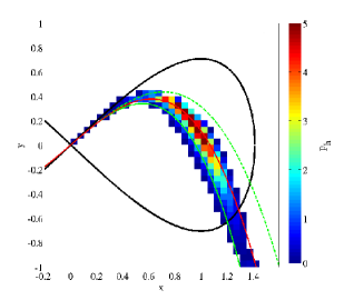
Figure 1: Escape path prehistory histogram for $\epsilon=0.1$ and $\sigma=0.3$ overlaid with the graphs of the third-order (solid, green line), fourth-order (dashed, green line), and fifth-order (solid, red line) center manifold equations given by Eq. (14a). The color-bar values have been normalized by $10^{5}$, and the threshold 0 value is about 9 000. Reproduced from Forgoston and Schwartz [5].

Figure 1 shows a histogram of escape path prehistory for $\epsilon=0.1$ and $\sigma=0.3$ (so that $D=\sigma^{2}/2=0.045$). The color-bar values of Fig. 1 have been normalized by $10^{5}$. The threshold $0$ value in the figure is actually about 9 000. Therefore, any histogram box containing less than 9 000 events shows up as white on the histogram. Overlaid on top of the histogram are the graphs of the third-order, fourth-order, and fifth-order center manifold equations. Each of these equations may be found by including terms of the appropriate order from Eq. (14a).

One can see from Fig. 1 that the third-order and fourth-order center manifolds essentially bound the entire region of escape path prehistory, while the fifth-order manifold lies along the region of highest probability of escape. Although it is not shown, it should be noted that the optimal escape path (found using large fluctuation theory) associated with the third-order center manifold is a heteroclinic orbit from $x=\sqrt{1-\epsilon+2\epsilon^{2}}$ to $x=0$ that lies directly on top of a section of the third-order center manifold (solid, green line in Fig. 1). Similarly, the optimal escape paths associated with higher order center manifolds lie directly on top of a section of the corresponding center manifold.

Additionally, one could overlay the histogram of escape path prehistory with the average stochastic center manifold given by Eq. (2). However, since the stochastic correction appears at order $\mathcal{O}(\epsilon^{4}\sigma^{2})$, there is no noticeable difference from the manifolds shown in Fig. 1. Therefore, plots of the average stochastic manifold are not shown.

Although corrections due to noise occur at high order in the current example, other problems with quadratic nonlinearities have noise corrections occurring at much lower order [33], as seen in the following example. In such cases, one must use the normal form coordinate transform method rather than relying on the deterministic center manifold reduction.

4 Example 2: Stochastic SEIR Epidemiological Model

The interaction between deterministic and stochastic effects in population dynamics has played, and continues to play, an important role in the modeling of infectious diseases. The mechanistic modeling side of population dynamics is well-known and established [34, 35]. These models typically are assumed to be useful for infinitely large, homogeneous populations, and arise from the mean field analysis of probabilistic models. On the other hand, when one considers finite populations, random interactions give rise to internal noise effects, which may introduce new dynamics. Stochastic effects are quite prominent in finite populations, which can range from ecological dynamics [36] to childhood epidemics in cities [37, 38]. For homogeneous populations with seasonal forcing, noise also comes into play in the prediction of large outbreaks [39, 40, 41]. Specifically, external random perturbations change the probabilistic prediction of epidemic outbreaks as well as its control [42].

As a first study, we consider the Susceptible-Exposed-Infected-Recovered (SEIR) epidemiological model with stochastic forcing. We could easily consider a very high-dimensional SEIR-type model where the exposed class was modeled using hundreds of compartments. Since the analysis is similar, we consider the simpler standard SEIR model to demonstrate the power of the method.

We begin by describing the stochastic version of the SEIR model found in Schwartz and Smith [43]. We assume that a given population may be divided into the following four classes which evolve in time:

1. Susceptible class, $s(t)$, consists of those individuals who may contract the disease.

2. Exposed class, $e(t)$, consists of those individuals who have been infected by the disease but are not yet infectious.

3. Infectious class, $i(t)$, consists of those individuals who are capable of transmitting the disease to susceptible individuals.

4. Recovered class, $r(t)$, consists of those individuals who are immune to the disease.

Furthermore, we assume that the total population size, denoted as $N$, is constant and can be normalized to $S(t)+E(t)+I(t)+R(t)=1$, where $S(t)=s(t)/N$, $E(t)=e(t)/N$, $I(t)=i(t)/N$, and $R(t)=r(t)/N$. Therefore, the population class variables $S$, $E$, $I$, and $R$ represent fractions of the total population. The governing equations for the stochastic SEIR model are

$$\dot{S}(t)=\mu-\beta I(t)S(t)-\mu S(t)+\sigma_{1}\phi_{1}(t),$$ (27a)

$$\dot{E}(t)=\beta I(t)S(t)-(\alpha+\mu)E(t)+\sigma_{2}\phi_{2}(t),$$ (27b)

$$\dot{I}(t)=\alpha E(t)-(\gamma+\mu)I(t)+\sigma_{3}\phi_{3}(t),$$ (27c)

$$\dot{R}(t)=\gamma I(t)-\mu R(t)+\sigma_{4}\phi_{4}(t),$$ (27d)

where $\sigma_{i}$ is the standard deviation of the noise intensity $D_{i}=\sigma_{i}^{2}/2$. Each of the noise terms, $\phi_{i}$, describes a stochastic, Gaussian white force that is characterized by the correlation functions given by Eqs. (10a)-(10b).

Additionally, $\mu$ represents a constant birth and death rate, $\beta$ is the contact rate, $\alpha$ is the rate of infection, so that $1/\alpha$ is the mean latency period, and $\gamma$ is the rate of recovery, so that $1/\gamma$ is the mean infectious period. Although the contact rate $\beta$ could be given by a time-dependent function (e.g. due to seasonal fluctuations), for simplicity, we assume $\beta$ to be constant. Throughout this article, we use the following parameter values: $\mu=0.02({\rm year})^{-1}$, $\beta=1575.0({\rm year})^{-1}$, $\alpha=1/0.0279({\rm year})^{-1}$, and $\gamma=1/0.01({\rm year})^{-1}$. Disease parameters correspond to typical measles values [43, 44]. Note that any other biologically meaningful parameters may be used as long as the basic reproductive rate $R_{0}=\alpha\beta/[(\alpha+\mu)(\gamma+\mu)]>1$. The interpretation of $R_{0}$ is the number of secondary cases produced by a single infectious individual in a population of susceptibles in one infectious period.

As a first approximation of stochastic effects, we have considered additive noise. This type of noise may result from migration into and away from the population being considered [45]. Since it is difficult to estimate fluctuating migration rates [46], it is appropriate to treat migration as an arbitrary external noise source. Also, fluctuations in the birth rate manifest itself as additive noise. Furthermore, as we are not interested in extinction events in this article, it is not necessary to use multiplicative noise. In general, for the problem considered here, it is possible that a rare event in the tail of the noise distribution may cause one or more of the $S$, $E$, and $I$ components of the solution to become negative. Here, we will always assume that the noise is sufficiently small so that a solution remains positive for a long enough time to gather sufficient statistics. Even though it is difficult to accurately estimate the appropriate noise level from real data, our choices of noise intensity lie within the huge confidence intervals computed in Bjørnstad et al [46].

Although $S+E+I+R=1$ in the deterministic system, one should note that the dynamics of the stochastic SEIR system will not necessarily have all of the components sum to unity. However, since the noise has zero mean, the total population will remain close to unity on average. Therefore, we assume that the dynamics are sufficiently described by Eqs. (27a)-(27c). It should be noted that even if $E(t)+I(t)=0$ for some $t$, the noise allows for the re-emergence of the epidemic.

1 Deterministic center manifold analysis

As seen in Sec. 1 one can reduce the dimension of a system of equations using deterministic center manifold theory. In order to make use of the center manifold theory, we transform the deterministic version of Eqs. (27a)-(27c) to a new system of equations that has the necessary spectral structure. The theory will allow us to find an invariant center manifold passing through the fixed point to which we can restrict the transformed system.

The transformed evolution equations are given by

$$\frac{dU}{d\tau}= -\alpha_{0}U+{\frac{\mu^{2}\left(\gamma_{0}V-\alpha_{0}U\right)}{\alpha_{0}+\gamma_{0}}}-{\frac{\left(\gamma_{0}+\mu^{2}\right)\left(\alpha_{0}+\mu^{2}\right)\left[\left(\alpha_{0}+\gamma_{0}\right)U+\gamma_{0}W\right]}{\alpha_{0}\left(\alpha_{0}+\gamma_{0}\right)}}$$

$$-\frac{\mu\beta}{\alpha_{0}+\gamma_{0}}\left(\gamma_{0}W+\left(\alpha_{0}+\gamma_{0}\right)U+{\frac{\mu^{2}\alpha_{0}\gamma_{0}}{\left(\gamma_{0}+\mu^{2}\right)\left(\alpha_{0}+\mu^{2}\right)}}\right)\left(U+V\right),$$ (28a)

$$\frac{dV}{d\tau}= \alpha_{0}U-{\frac{\mu^{2}\left(\gamma_{0}V-\alpha_{0}U\right)}{\alpha_{0}+\gamma_{0}}}-{\frac{\left(\gamma_{0}+\mu^{2}\right)\left(\alpha_{0}+\mu^{2}\right)\left[\left(\alpha_{0}+\gamma_{0}\right)U+\gamma_{0}W\right]}{\gamma_{0}\left(\alpha_{0}+\gamma_{0}\right)}}$$

$$-\frac{\mu\beta\alpha_{0}}{\gamma_{0}\left(\alpha_{0}+\gamma_{0}\right)}\left(\gamma_{0}W+\left(\alpha_{0}+\gamma_{0}\right)U+{\frac{\mu^{2}\alpha_{0}\gamma_{0}}{\left(\gamma_{0}+\mu^{2}\right)\left(\alpha_{0}+\mu^{2}\right)}}\right)\left(U+V\right),$$ (28b)

$$\frac{dW}{d\tau}= -\alpha_{0}U-\left(\gamma_{0}+\mu^{2}\right)\left(U+W\right)+{\frac{\left(\gamma_{0}+\mu^{2}\right)\left(\alpha_{0}+\mu^{2}\right)\left[\left(\alpha_{0}+\gamma_{0}\right)U+\gamma_{0}W\right]}{\alpha_{0}\gamma_{0}}}$$

$$-\mu^{2}V+\frac{\mu\beta}{\gamma_{0}}\left(\gamma_{0}W+\left(\alpha_{0}+\gamma_{0}\right)U+{\frac{\mu^{2}\alpha_{0}\gamma_{0}}{\left(\gamma_{0}+\mu^{2}\right)\left(\alpha_{0}+\mu^{2}\right)}}\right)\left(U+V\right),$$ (28c)

$$\frac{d\mu}{d\tau}= 0,$$ (28d)

where

$$U=\frac{-\gamma_{0}}{\alpha_{0}+\gamma_{0}}\bar{E},$$ (29a)

$$V=\bar{S}+\frac{\gamma_{0}}{\alpha_{0}+\gamma_{0}}\bar{E},$$ (29b)

$$W=\bar{I}+\bar{E},$$ (29c)

$\bar{S}(t)=S(t)-S_{0}$, $\bar{E}(t)=E(t)-E_{0}$, and $\bar{I}(t)=I(t)-I_{0}$,

$$(S_{0},E_{0},I_{0})=\left({\frac{\left(\gamma+\mu\right)\left(\alpha+\mu\right)}{\beta\alpha}},{\frac{\mu}{\alpha+\mu}}-{\frac{\mu\left(\gamma+\mu\right)}{\alpha\beta}},{\frac{\mu\alpha}{\left(\gamma+\mu\right)\left(\alpha+\mu\right)}}-{\frac{\mu}{\beta}}\right)$$ (30)

is a fixed point corresponding to the endemic state, and $\alpha=\alpha_{0}/\mu$ and $\gamma=\gamma_{0}/\mu$, where $\alpha_{0}$ and $\gamma_{0}$ are $\mathcal{O}(1)$. Details regarding the transformation can be found in Forgoston et al [33].

The Jacobian of Eqs. (28)-(LABEL:e:dmu_mort) to zeroth-order in $\mu$ and evaluated at the origin is

$$\left[\begin{array}[]{cc|ccccccccc}-(\alpha_{0}+\gamma_{0})&&&&0&&&-\frac{\gamma_{0}^{2}}{(\alpha_{0}+\gamma_{0})}&&&0\\ &&&&&&&&&&\\ \hline\cr&&&&&&&&&&\\ 0&&&&0&&&-\frac{\alpha_{0}\gamma_{0}}{(\alpha_{0}+\gamma_{0})}&&&0\\ &&&&&&&&&&\\ 0&&&&0&&&0&&&0\\ &&&&&&&&&&\\ 0&&&&0&&&0&&&0\end{array}\right],$$ (31)

which shows that Eqs. (28)-(LABEL:e:dmu_mort) may be rewritten in the form

$$\frac{d{\bf x}}{d\tau}={\bf A}{\bf x}+{\bf f}({\bf x},{\bf y},\mu),$$ (32)

$$\frac{d{\bf y}}{d\tau}={\bf B}{\bf y}+{\bf g}({\bf x},{\bf y},\mu),$$ (33)

$$\frac{d\mu}{d\tau}=0,$$ (34)

where ${\bf x}=(U)$, ${\bf y}=(V,W)$, ${\bf A}$ is a constant matrix with eigenvalues that have negative real parts, ${\bf B}$ is a constant matrix with eigenvalues that have zero real parts, and ${\bf f}$ and ${\bf g}$ are nonlinear functions in ${\bf x}$, ${\bf y}$ and $\mu$. In particular,

$${\bf A}=\left[\begin{array}[]{c}-(\alpha_{0}+\gamma_{0})\end{array}\right],\,\,\,\,\,\,\,\,\,\,\,\,\,\,\,{\bf B}=\left[\begin{array}[]{cccc}0&&&-\frac{\alpha_{0}\gamma_{0}}{(\alpha_{0}+\gamma_{0})}\\ &&&\\ 0&&&0\end{array}\right].$$ (35)

Therefore, the system will rapidly collapse onto a lower-dimensional manifold given by center manifold theory [20]. Furthermore, we know that the center manifold is given by

$$U=h(V,W,\mu),$$ (36)

where $h$ is an unknown function.

Substitution of Eq. (36) into Eq. (28) leads to the following center manifold condition:

$$\frac{\partial h(V,W,\mu)}{\partial V}\frac{dV}{d\tau}+\frac{\partial h(V,W,\mu)}{\partial W}\frac{dW}{d\tau}=-\alpha_{0}h(V,W,\mu)+{\frac{\mu^{2}\left[\gamma_{0}V-\alpha_{0}h(V,W,\mu)\right]}{\alpha_{0}+\gamma_{0}}}-$$

$${\frac{\left(\gamma_{0}+\mu^{2}\right)\left(\alpha_{0}+\mu^{2}\right)\left[\left(\alpha_{0}+\gamma_{0}\right)h(V,W,\mu)+\gamma_{0}W\right]}{\alpha_{0}\left(\alpha_{0}+\gamma_{0}\right)}}-$$

$$\frac{\mu\beta}{\alpha_{0}+\gamma_{0}}\left(\gamma_{0}W+\left(\alpha_{0}+\gamma_{0}\right)h(V,W,\mu)+{\frac{\mu^{2}\alpha_{0}\gamma_{0}}{\left(\gamma_{0}+\mu^{2}\right)\left(\alpha_{0}+\mu^{2}\right)}}\right)\left(h(V,W,\mu)+V\right).$$ (37)

In general, it is not possible to solve the center manifold condition for the unknown function, $h(V,W,\mu)$. Therefore, we perform the following Taylor series expansion of $h(V,W,\mu)$ in $V$, $W$, and $\mu$:

$$h(V,W,\mu)= h_{0}+h_{2}V+h_{3}W+h_{\mu}\mu+h_{22}V^{2}+h_{23}VW+h_{33}W^{2}+$$

$$h_{\mu 2}\mu V+h_{\mu 3}\mu W+h_{\mu\mu}\mu^{2}+\ldots,$$ (38)

where $h_{0}$, $h_{2}$, $h_{3}$, $h_{\mu}$, $\ldots$ are unknown coefficients that are found by substituting the Taylor series expansion into the center manifold condition and equating terms of the same order. By carrying out this procedure using a second-order Taylor series expansion of $h$, the center manifold equation is

$$U=-\frac{\gamma_{0}^{2}}{(\alpha_{0}+\gamma_{0})^{2}}W+\mathcal{O}(\epsilon^{3}),$$ (39)

where $\epsilon=|(V,W,\mu)|$ so that $\epsilon$ provides a count of the number of $V$, $W$, and $\mu$ factors in any one term. Substitution of Eq. (39) into Eqs. (28) and (28d) leads to the following reduced system of evolution equations which describe the dynamics on the center manifold:

$$\frac{dV}{d\tau}= -{\frac{\mu^{2}{\gamma_{0}}^{2}\alpha_{0}W}{\left(\alpha_{0}+\gamma_{0}\right)^{3}}}-{\frac{\mu^{4}\alpha_{0}W}{\left(\alpha_{0}+\gamma_{0}\right)^{2}}}-{\frac{\gamma_{0}\mu^{2}V}{\alpha_{0}+\gamma_{0}}}-$$

$${\frac{\left(\gamma_{0}+\mu^{2}\right)\alpha_{0}W}{\alpha_{0}+\gamma_{0}}}-\frac{\beta{\alpha_{0}}^{2}\mu}{\left(\alpha_{0}+\gamma_{0}\right)^{2}}\left(W+{\frac{\mu^{2}\left(\alpha_{0}+\gamma_{0}\right)}{\left(\gamma_{0}+\mu^{2}\right)\left(\alpha_{0}+\mu^{2}\right)}}\right)\left(V-{\frac{{\gamma_{0}}^{2}W}{\left(\alpha_{0}+\gamma_{0}\right)^{2}}}\right),$$ (40a)

$$\frac{dW}{d\tau}= {\frac{\mu^{2}{\gamma_{0}}^{2}W}{\left(\alpha_{0}+\gamma_{0}\right)^{2}}}+{\frac{\mu^{4}W}{\alpha_{0}+\gamma_{0}}}-\mu^{2}V+$$

$$\frac{\beta\mu\alpha_{0}}{\alpha_{0}+\gamma_{0}}\left(W+{\frac{\mu^{2}\left(\alpha_{0}+\gamma_{0}\right)}{\left(\gamma_{0}+\mu^{2}\right)\left(\alpha_{0}+\mu^{2}\right)}}\right)\left(V-{\frac{{\gamma_{0}}^{2}W}{\left(\alpha_{0}+\gamma_{0}\right)^{2}}}\right).$$ (40b)

2 Projection of the noise onto the stochastic center manifold

The stochastic SEIR system given by Eqs. (27a)-(27c) may be transformed in a manner similar to what was done in the preceding section for the deterministic form of the system. The transformation will have an effect on the noise terms. The transformed stochastic terms are still additive, Gaussian noise processes. However, the transformation has acted on the original stochastic terms $\phi_{1}$, $\phi_{2}$, and $\phi_{3}$ to create new noise processes which have a variance different from that of the original noise processes. This transformed system of equations is an exact transformation of the system of equations given by Eqs. (27a)-(27c) and can be found in Forgoston et al [33].

Reduction of the stochastic SEIR model

It is tempting to consider the reduced stochastic model found by substitution of Eq. (39) into the tranformed equations, so that one has the following stochastic evolution equations (that hopefully describe the dynamics on the stochastic center manifold):

$$\frac{dV}{d\tau}= -{\frac{\mu^{2}{\gamma_{0}}^{2}\alpha_{0}W}{\left(\alpha_{0}+\gamma_{0}\right)^{3}}}-{\frac{\mu^{4}\alpha_{0}W}{\left(\alpha_{0}+\gamma_{0}\right)^{2}}}-{\frac{\gamma_{0}\mu^{2}V}{\alpha_{0}+\gamma_{0}}}-{\frac{\left(\gamma_{0}+\mu^{2}\right)W\alpha_{0}}{\alpha_{0}+\gamma_{0}}}-$$

$$\frac{\beta{\alpha_{0}}^{2}\mu}{\left(\alpha_{0}+\gamma_{0}\right)^{2}}\left(W+{\frac{\mu^{2}\left(\alpha_{0}+\gamma_{0}\right)}{\left(\gamma_{0}+\mu^{2}\right)\left(\alpha_{0}+\mu^{2}\right)}}\right)\left(V-{\frac{{\gamma_{0}}^{2}W}{\left(\alpha_{0}+\gamma_{0}\right)^{2}}}\right)+\sigma_{5}\phi_{5},$$ (41a)

$$\frac{dW}{d\tau}= {\frac{\mu^{2}{\gamma_{0}}^{2}W}{\left(\alpha_{0}+\gamma_{0}\right)^{2}}}+{\frac{\mu^{4}W}{\alpha_{0}+\gamma_{0}}}-\mu^{2}V+$$

$$\frac{\beta\mu\alpha_{0}}{\alpha_{0}+\gamma_{0}}\left(W+{\frac{\mu^{2}\left(\alpha_{0}+\gamma_{0}\right)}{\left(\gamma_{0}+\mu^{2}\right)\left(\alpha_{0}+\mu^{2}\right)}}\right)\left(V-{\frac{{\gamma_{0}}^{2}W}{\left(\alpha_{0}+\gamma_{0}\right)^{2}}}\right)+\sigma_{6}\phi_{6},$$ (41b)

where

$$\sigma_{5}\phi_{5}= \mu\sigma_{1}\phi_{1}+\frac{\mu\gamma_{0}}{\alpha_{0}+\gamma_{0}}\sigma_{2}\phi_{2},$$ (42a)

$$\sigma_{6}\phi_{6}= \mu\sigma_{2}\phi_{2}+\mu\sigma_{3}\phi_{3}$$ (42b)

are transformed stochastic terms.

One should note that Eqs. (41a)-(41b) also can be found by naïvely adding the stochastic terms to the reduced system of evolution equations for the deterministic problem (Eqs. (40a)-(40b)). This type of stochastic center manifold reduction has been done for the case of discrete noise [44]. Additionally, in many other fields (e.g. oceanography, solid mechanics, fluid mechanics), researchers have performed stochastic model reduction using a Karhunen-Loève expansion (principal component analysis, proper orthogonal decomposition) [47, 48]. However, this linear projection does not properly capture the nonlinear effects. Furthermore, one must subjectively choose the number of modes needed for the expansion. Therefore, even though the solution to the reduced model found using this technique may have the correct statistics, individual solution realisations will not agree with the original, complete solution.

It can be seen in Fig. 2 that Eqs. (41a)-(41b) do not contain the correct projection of the noise onto the center manifold. Therefore, when solving the reduced system, one does not obtain the correct solution. Such errors in stochastic epidemic modeling impact the prediction of disease outbreak when modeling the spread of a disease in a population.

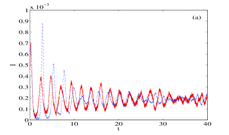
Figure 2: Time series of the fraction of the population that is infected with a disease, $I$, computed using the complete, stochastic system of transformed equations of the SEIR model (red, solid line), and computed using the reduced system of equations of the SEIR model that is based on the deterministic center manifold with a replacement of the noise terms (Eqs. (41a)-(41b)) (blue, dashed line). The standard deviation of the noise intensity used in the simulation is $\sigma_{i}=0.0005$, $i=4,5,6$. The time series is shown for (a) $t=0$ to $t=40$, and for (b) $t=40$ to $t=100$. Reproduced from Forgoston et al [33].

Figures 2(a)-(b) compares the time series of the fraction of the population that is infected with a disease, $I$, computed using the complete, stochastic system of transformed equations of the SEIR model with the time series of $I$ computed using the reduced system of equations of the SEIR model that is based on the deterministic center manifold with a replacement of the noise terms (Eqs. (41a) and (41b)). Figure 2(a) shows the initial transients, while Fig. 2(b) shows the time series after the transients have decayed. One can see that the solution computed using the reduced system quickly becomes out of phase with the solution of the complete system. Use of this reduced system would lead to an incorrect prediction of the initial disease outbreak. Additionally, the predicted amplitude of the initial outbreak would be incorrect. The poor agreement, both in phase and amplitude, between the two solutions continues for long periods of time as seen in Fig. 2(b). We also have computed the cross-correlation of the two time series shown in Fig. 2(a)-(b) to be approximately 0.34. Since the cross-correlation measures the similarity between the two time series, this low value quantitatively suggests poor agreement between the two solutions.

Correct projection of the noise onto the stochastic center manifold

To project the noise correctly onto the center manifold, we derive a normal form coordinate transform using the principles of Sec. 2 for the complete, stochastic system of transformed equations of the SEIR model.

The stochastic system of equations (which satisfies the necessary spectral requirements) in $\left(U,V,W\right)^{T}$ coordinates is transformed to a new $\left(Y,X_{1},X_{2}\right)^{T}$ coordinate system using a near-identity stochastic coordinate transform given as

$$U= Y+\xi\left(Y,X_{1},X_{2},\tau\right),$$ (43a)

$$V= X_{1}+\eta\left(Y,X_{1},X_{2},\tau\right),$$ (43b)

$$W= X_{2}+\rho\left(Y,X_{1},X_{2},\tau\right),$$ (43c)

where the specific form of $\xi\left(Y,X_{1},X_{2},\tau\right)$, $\eta\left(Y,X_{1},X_{2},\tau\right)$, and $\rho\left(Y,X_{1},X_{2},\tau\right)$ is found using an iterative procedure.

Several iterations lead to coordinate transforms for $U$, $V$, and $W$ along with evolution equations describing the $Y$-dynamics, $X_{1}$-dynamics, and $X_{2}$-dynamics in the new coordinate system. The $Y$-dynamics have exponential decay to the $Y=0$ slow manifold. Substitution of $Y=0$ leads to complicated expressions for the coordinate transforms - they can be found in Forgoston et al [33].

We are interested in the long-term slow processes. Since the memory integrals are fast-time processes, we neglect them along with the higher-order multiplicative terms to obtain the following expressions for $U$, $V$, and $W$:

$$U= -\frac{\gamma_{0}^{2}X_{2}}{\left(\alpha_{0}+\gamma_{0}\right)^{2}}-\frac{\mu\beta X_{1}}{\left(\alpha_{0}+\gamma_{0}\right)}\left(\frac{\mu^{2}}{\left(\alpha_{0}+\gamma_{0}\right)}+\frac{\gamma_{0}X_{2}}{\left(\alpha_{0}+\gamma_{0}\right)}+\mu^{2}X_{2}\right)$$

$$+\frac{\mu^{2}\gamma_{0}}{\left(\alpha_{0}+\gamma_{0}\right)}\left(X_{1}-\frac{2X_{2}}{\alpha_{0}}\right),$$ (44a)

$$V= ~{}X_{1},$$ (44b)

$$W= ~{}X_{2}.$$ (44c)

Note that Eq. (44a) is the deterministic center manifold equation, and at first-order, matches the center manifold equation that was found previously (Eq. (39)).

Substitution of $Y=0$ and neglecting all multiplicative noise terms and memory integrals using the argument from above (so that we consider only first-order noise terms) leads to the following reduced system of evolution equations on the center manifold:

$$\frac{dX_{1}}{d\tau}=F(X_{1}(\tau),X_{2}(\tau)),$$ (45a)

$$\frac{dX_{2}}{d\tau}=G(X_{1}(\tau),X_{2}(\tau)).$$ (45b)

The specific form of $F$ and $G$ in Eqs. (45a) and (45b) are complicated, and can be found in Forgoston et al [33].

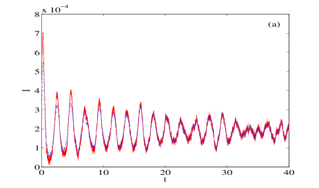
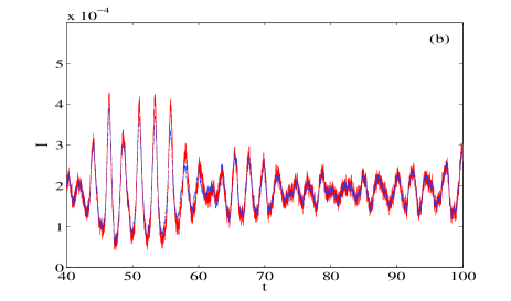
Figure 3: Time series of the fraction of the population that is infected with a disease, $I$, computed using the complete, stochastic system of transformed equations of the SEIR model (red, solid line), and computed using the reduced system of equations of the SEIR model that is found using the stochastic normal form coordinate transform (Eqs. (45a)-(45b)) (blue, dashed line). The standard deviation of the noise intensity used in the simulation is $\sigma_{i}=0.0005$, $i=4,5,6$. The time series is shown for (a) $t=0$ to $t=40$, and for (b) $t=40$ to $t=100$. Reproduced from Forgoston et al [33].

Figures 3(a)-(b) compares the time series of the fraction of the population that is infected with a disease, $I$, computed using the complete, stochastic system of transformed equations of the SEIR model with the time series of $I$ computed using the reduced system of equations of the SEIR model that is found using the stochastic normal form coordinate transform (Eqs. (45a)-(45b)). Figure 3(a) shows the initial transients, while Fig. 3(b) shows the time series after the transients have decayed. One can see that there is excellent agreement between the two solutions. The initial outbreak is successfully captured by the reduced system. Furthermore, Fig. 3(b) shows that the reduced system accurately predicts recurrent outbreaks for a time scale that is orders of magnitude longer than the relaxation time. This is not surprising since the solution decays exponentially throughout the transient and then remains close to the lower-dimensional center manifold. Since we are not looking at periodic orbits, there are no secular terms in the asymptotic expansion, and the result is valid for all time. Additionally, any noise drift on the center manifold results in bounded solutions due to sufficient dissipation transverse to the manifold. The cross-correlation of the two time series shown in Fig. 3 is approximately 0.98, which quantitatively suggests there is excellent agreement between the two solutions.

Unlike example 1, where the average stochastic center manifold and deterministic center manifold are virtually identical, the SEIR model considered in example 2 has terms at low order in the normal form transform which cause a significant difference between the average stochastic center manifold and the deterministic manifold. Therefore, as we have demonstrated, when working with the SEIR model, one must use the normal form coordinate transform method to correctly project the noise onto the center manifold.

5 Conclusions

This review highlights some of our results in stochastic model reduction that use the normal form coordinate transform method of A.J. Roberts. It is increasingly apparent that small external effects can play a significant role in the dynamics of models used for real world applications. Therefore, researchers are revisiting existing methods and developing new ones to quantify noise-induced phenomena in stochastic models. Time series prediction is a classic problem in deterministic dynamical systems. As we develop methods to approach its counterpart in stochastic models, we recognize the limitations of high dimensional analysis. Moreover, many techniques that are probabilistic in nature for stochastic systems can be carried over to deterministic complex systems, such as chaos or turbulence. Reduced models provide tractable systems to analyze and test, both analytically and computationally. However, there is still much work to be done in moving to high-dimensional systems, including dynamics on large-scale heterogeneous networks where mean field analysis typically fails [11], and truly infinite stochastic systems arising from delay [49], where the force of the noise needs to be known in the past and future.

In this work, we demonstrate the importance of properly projecting the noise source through the reduction. The method of Roberts is an important contribution as it not only enables one to reduce the dimensionality of the dynamics, but also provides a way to separate all slow processes from all fast processes. We have demonstrated in these two examples how deriving the deterministic manifold may not be sufficient, and in this case, how one can employ the normal form coordinate transform method to properly capture the stochastic manifold. The result in the SEIR example is a closed form system that can be analyzed and tested for extended time series prediction. Stochastic model reduction is a general approach that can be used to analyze the dynamics of generic stochastic models with separated time scales.

Acknowledgments

EF and LB are supported by the National Science Foundation award DMS #1418956. IBS is funded under the Office of Naval Research award N0001412WX20083, and the NRL Base Research Program N0001412WX30002.

We thank Tony (A.J. Roberts) for his conversations, comments and insight over the years regarding the work presented in this article.

References

- 1. M. I. Dykman, Large fluctuations and fluctuational transitions in systems driven by coloured gaussian noise: A high-frequency noise, Phys. Rev. A. 42, 2020–2029, (1990).
- 2. M. I. Dykman, P. V. E. McClintock, V. N. Smelyanski, N. D. Stein, and N. G. Stocks, Optimal paths and the prehistory problem for large fluctuations in noise-driven systems, Phys. Rev. Lett. 68, 2718–2721, (1992).
- 3. M. Millonas, Ed., Fluctuations and Order: The New Synthesis. (Springer-Verlag, 1996).
- 4. D. G. Luchinsky, P. V. E. McClintock, and M. I. Dykman, Analogue studies of nonlinear systems, Rep. Prog. Phys. 61, 889–997, (1998).
- 5. E. Forgoston and I. B. Schwartz, Escape rates in a stochastic environment with multiple scales, SIAM J. Appl. Dyn. Syst. 8(3), 1190–1217, (2009).
- 6. R. V. Kohn, M. G. Reznikoff, and E. Vanden-Eijnden, Magnetic elements at finite temperature and large deviation theory, J. Nonlinear Sci. 15, 223–253, (2005).
- 7. T. A. Fulton and L. N. Dunkelberger, Lifetime of the zero-voltage state in Josephson tunnel junctions, Phys. Rev. B. 9, 4760, (1974).
- 8. L. S. Tsimring, Noise in biology, Reports on Progress in Physics. 77(2), 026601, (2014).
- 9. M. Assaf, E. Roberts, and Z. Luthey-Schulten, Determining the stability of genetic switches: Explicitly accounting for mRNA noise, Phys. Rev. Lett. 106, 248102, (2011).
- 10. B. S. Lindley, L. B. Shaw, and I. B. Schwartz, Rare-event extinction on stochastic networks, EPL. 108, 58008, (2014).
- 11. J. H. Schwartz and I. B., Epidemic extinction and control in heterogeneous networks, PHYSICAL REVIEW LETTERS. 117, 028302, (2016).
- 12. J. Hindes and I. B. Schwartz, Epidemic extinction paths in complex networks, Physical Review E. 95(5), 052317, (2017).
- 13. J. Hindes and I. B. Schwartz, Large order fluctuations, switching, and control in complex networks, Scientific Reports. 7(1), 10663, (2017).
- 14. E. Roberts, S. Be’er, C. Bohrer, R. Sharma, and M. Assaf, Dynamics of simple gene-network motifs subject to extrinsic fluctuations, Phys. Rev. E. 92, 062717, (2015).
- 15. A. J. Roberts, Normal form transforms separate slow and fast modes in stochastic dynamical systems, Physica A. 387(1), 12–38 (January, 2008).
- 16. N. Berglund and B. Gentz, Geometric singular perturbation theory for stochastic differential equations, J. Differ. Equations. 191, 1–54, (2003).
- 17. N. Berglund and B. Gentz, Noise-induced phenomena in slow-fast dynamical systems: a sample-paths approach. (Springer Science & Business Media, 2006).
- 18. C. R. Heckman and I. B. Schwartz, Stochastic switching in slow-fast systems: A large-fluctuation approach, PHYSICAL REVIEW E. 89, 022919, (2014).
- 19. C. Chicone and Y. Latushkin, Center manifolds for infinite dimensional nonautonomous differential equations, J. Differ. Equations. 141, 356–399, (1997).
- 20. J. Carr, Applications of Centre Manifold Theory. (Springer-Verlag, 1981).
- 21. P. Boxler, A stochastic version of center manifold theory, Probab. Theory Rel. 83, 509–545, (1989).
- 22. E. Knobloch and K. A. Wiesenfeld, Bifurcations in fluctuating systems: The center-manifold approach, J. Stat. Phys. 33(3), 611–637, (1983).
- 23. P. H. Coullet, C. Elphick, and E. Tirapegui, Normal form of a Hopf bifurcation with noise, Phys. Lett. A. 111, 277–282, (1985).
- 24. N. S. Namachchivaya, Stochastic bifurcation, Appl. Math. Comput. 38, 101–159, (1990).
- 25. N. S. Namachchivaya and Y. K. Lin, Method of stochastic normal forms, Int. J. Nonlinear Mech. 26, 931–943, (1991).
- 26. L. Arnold and P. Imkeller, Normal forms for stochastic differential equations, Probab. Theory Rel. 110, 559–588, (1998).
- 27. L. Arnold, Random Dynamical Systems. (Springer-Verlag, 1998).
- 28. D. C. Webb, P. J. Simonetti, and C. P. Jones, Slocum: An underwater glider propelled by environmental energy, IEEE J. Oceanic Eng. 26, 447–452, (2001).
- 29. J. Sherman, R. E. Davis, W. B. Owens, and J. Valdes, The autonomous underwater glider ’Spray’, IEEE J. Oceanic Eng. 26, 437–446, (2001).
- 30. C. C. Eriksen, T. J. Osse, R. D. Light, T. Wen, T. W. Lehman, P. L. Sabin, J. W. Ballard, and A. M. Chiodi, Seaglider: A long-range autonomous underwater vehicle for oceanographic research, IEEE J. Oceanic Eng. 26, 424–436, (2001).
- 31. M. I. Freidlin and A. D. Wentzell, Random Perturbations of Dynamical Systems. (Springer-Verlag, 1984).
- 32. E. Forgoston and R. O. Moore, A primer on noise-induced transitions in applied dynamical systems, SIAM Review. (accepted).
- 33. E. Forgoston, L. Billings, and I. B. Schwartz, Accurate noise projection for reduced stochastic epidemic models, Chaos. 19, 043110, (2009).
- 34. R. M. Anderson and R. M. May, Infectious Diseases of Humans. (Oxford University Press, 1991).
- 35. N. T. J. Bailey, The Mathematical Theory of Infectious Diseases. (Charles Griffin, London, 1975).
- 36. G. Marion, E. Renshaw, and G. Gibson, Stochastic modelling of environmental variation for biological populations, Theor. Popul. Biol. 57(3), 197–217 (May, 2000).
- 37. H. T. H. Nguyen and P. Rohani, Noise, nonlinearity and seasonality: The epidemics of whooping cough revisited, J. Roy. Soc. Interface. 5(21), 403–413 (April, 2008).
- 38. P. Rohani, M. J. Keeling, and B. T. Grenfell, The interplay between determinism and stochasticity in childhood diseases, Am. Nat. 159(5), 469–481 (May, 2002).
- 39. D. A. Rand and H. B. Wilson, Chaotic stochasticity - A ubiquitous source of unpredictability in epidemics, P. Roy. Soc. B - Biol. Sci. 246(1316), 179–184 (November, 1991).
- 40. L. Billings, E. M. Bollt, and I. B. Schwartz, Phase-space transport of stochastic chaos in population dynamics of virus spread, Phys. Rev. Lett. 88, 234101, (2002).
- 41. L. Stone, R. Olinky, and A. Huppert, Seasonal dynamics of recurrent epidemics, Nature. 446, 533–536, (2007).
- 42. I. B. Schwartz, L. Billings, and E. M. Bollt, Dynamical epidemic suppression using stochastic prediction and control, Phys. Rev. E. 70, 046220, (2004).
- 43. I. Schwartz and H. Smith, Infinite subharmonic bifurcations in an SEIR epidemic model, J. Math. Biol. 18, 233–253, (1983).
- 44. L. Billings and I. B. Schwartz, Exciting chaos with noise: unexpected dynamics in epidemic outbreaks, J. Math. Biol. 44, 31–48, (2002).
- 45. F. Brauer, P. van den Driessche, and J. Wu, Eds., Mathematical Epidemiology. (Springer-Verlag, 2008).
- 46. O. N. Bjørnstad, B. F. Finkenstädt, and B. T. Grenfell, Dynamics of measles epidemics: Estimating scaling, Ecol. Monogr. 72(2), 169–184, (2002).
- 47. A. Doostan, R. G. Ghanem, and J. Red-Horse, Stochastic model reduction for chaos representations, Comput. Methods Appl. Mech. Engrg. 196, 3951–3966, (2007).
- 48. D. Venturi, X. Wan, and G. E. Karniadakis, Stochastic low-dimensional modelling of a random laminar wake past a circular cylinder, J. Fluid Mech. 606, 339–367, (2008).
- 49. I. B. Schwartz, L. Billings, T. W. Carr, and M. Dykman, Noise-induced switching and extinction in systems with delay, Physical Review E. 91(1), 012139, (2015).