Multiphoton excitation and high-harmonics generation in topological insulator

Abstract

Multiphoton interaction of coherent electromagnetic radiation with 2D metallic carriers confined on the surface of the 3D topological insulator is considered. A microscopic theory describing the nonlinear interaction of a strong wave and metallic carriers with many-body Coulomb interaction is developed. The set of integrodifferential equations for the interband polarization and carrier occupation distribution is solved numerically. Multiphoton excitation of Fermi-Dirac sea of 2D massless carriers is considered for a THz pump wave. It is shown that in the moderately strong pump wave field along with multiphoton interband/intraband transitions the intense radiation of high harmonics takes place.

1 Introduction

Along with graphene topological insulators (TI) recently emerged as a central theme in condensed matter physics [1, 2]. Three-dimensional TIs are bulk insulators endowed with a topological invariant that manifests itself through robust 2D metallic surface states. These states are helical with massless linear Dirac like energy dispersion, that is, each surface-momentum state possesses a unique spin direction and are protected against backscattering by time-reversal symmetry [3, 4]. The unique properties of the surface states are responsible for their exotic electromagnetic properties. Several theoretical works on light-TI interaction have illustrated interesting effects [5, 6, 7, 8, 9]. Experimentally, Kerr [10] and Faraday [11] effects, and second-harmonic generation [12] process in TI have been studied. Metallic surface states being Dirac like are responsible for strong nonlinear terahertz response of TI  [13, 14, 15], and like to graphene TIs have great potential as an effective nonlinear optical material [16]. In particular, in the strong pump field limit, one can realize the regime where multiphoton effects are essential [17, 18, 19] and high-harmonics are generated. The experiment [20] with the generation of ninth harmonic in graphene opens new avenue towards high-harmonic generation in 2D nanostructures. Hence it is of interest to investigate multiphoton excitation and subsequent high harmonic generation process in TIs.

In the present work, we develop a nonlinear microscopic quantum theory of interaction of 2D metallic carriers confined on the surface of the 3D TI (e.g. Bi₂Se₃) with coherent electromagnetic radiation. We also take into account electron-electron Coulomb interaction with induced many-body effects. We consider nonlinear coherent interaction in the ultrafast excitation regime when relaxation processes due to electron-phonon coupling via longitudinal surface phonons are not relevant. We use the self-consistent Hartree-Fock approximation that leads to a closed set of integrodifferential equations for the interband polarization and carrier occupation distribution. The latter is solved numerically. Then we consider high harmonic generation process for strong pump waves and show that one can achieve efficient generation of high harmonics in TIs.

The paper is organized as follows. In Sec. II the set of equations for the interband polarization and carrier occupation distribution is formulated. In Sec. III, we consider multiphoton excitation of Fermi-Dirac sea and generation of harmonics in TI. Finally, conclusions are given in Sec. IV.

2 Evolutionary equation for single-particle density matrix

Low-energy excitations of 2D metallic surface states of TI which are much smaller than the bulk gap energy ($0.3\ \mathrm{eV}$ for $\mathrm{Bi}_{2}\mathrm{Se}_{3}$) can be described by the effective Hamiltonian

$$H_{0}=\hbar\mathrm{v}_{F}\left(k_{x}\sigma_{y}-k_{y}\sigma_{x}\right)=i\hbar\mathrm{v}_{F}\left(\begin{array}[]{cc}0&-k_{x}+ik_{y}\\ k_{x}+ik_{y}&0\end{array}\right),$$ (1)

where $\mathrm{v}_{F}\approx c/450$ is the Fermi velocity for the topological insulator ($c$ is the light speed in vacuum), $\hbar\mathbf{k}$ is the 2D electron momentum operator. The Pauli matrices $\sigma_{x}$ and $\sigma_{y}$ act in the real electron spin space. The eigenstates of the effective Hamiltonian (1) are

$$|\psi_{\eta,\mathbf{k}}(\mathbf{r})\rangle=\frac{1}{\sqrt{\mathcal{A}}}|\varphi_{\eta,\mathbf{k}}\rangle e^{i\mathbf{kr}},$$ (2)

where the spinors

$$|\varphi_{\eta,\mathbf{k}}\rangle=\frac{1}{\sqrt{2}}\left(\begin{array}[]{c}e^{-i\theta\left(\mathbf{k}\right)}\\ i\eta\end{array}\right)$$

correspond to energies

$$\mathcal{E}_{\eta}\left(\mathbf{k}\right)=\eta\hbar\mathrm{v}_{F}k.$$

Here for conduction band $\eta=1$ and for valence band $\eta=-1$, $\mathcal{A}$ is the surface area, and

$$\theta\left(\mathbf{k}\right)=\arctan\left(\frac{k_{y}}{k_{x}}\right)$$ (3)

is the polar angle in the momentum space. The mean value of an electron spin in the 2D surface states of TI is

$$\frac{\hbar}{2}\langle\psi_{\eta,\mathbf{k}}|\mathbf{\sigma}|\psi_{\eta,\mathbf{k}}\rangle=\frac{\eta\hbar}{2}\left[\widehat{\mathbf{z}}\times\widehat{\mathbf{k}}\right],$$ (4)

where $\widehat{\mathbf{k}}$ and $\widehat{\mathbf{z}}$ are unit vectors directed along the $\mathbf{k}$ and the $z$-axis (normal to the surface), respectively. As is seen from Eq. (4), in TI the spin of electron lies in the surface plane and is perpendicular to its momentum. At that, for conduction band it is directed in the counterclockwise direction and inversely for the valence band.

Let a plane linearly polarized (along the $x$-axis) quasimonochromatic electromagnetic radiation of carrier frequency $\omega_{0}$ and slowly varying envelope $E_{0}(t)$ interacts with the 3D TI. We assume perpendicular to the metallic surface incidence and $\hbar\omega_{0}<<\mathcal{E}_{g}$ ($\mathcal{E}_{g}$ is the TI’s bulk gap). Besides, we will restrict wave intensity to forbidden transition within the bulk bands. Under these circumstances, one can neglect bulk excitations and the nonlinear electromagnetic response of TI will be conditioned by the 2D surface states. Thus, the light–TI interaction Hamiltonian in the length gauge will be:

$$\widehat{H}_{\mathrm{int}}=e\int d\mathbf{r}\ \widehat{\Psi}^{\dagger}(\mathbf{r})\mathbf{rE}\left(t\right)\widehat{\Psi}(\mathbf{r}),$$ (5)

where $\widehat{\Psi}(\mathbf{r})$ is the fermionic field operator and

$$\mathbf{E}\left(t\right)=\widehat{\mathbf{x}}E_{0}\left(t\right)\cos\omega_{0}t.$$ (6)

We will work in the second quantization formalism using the Fermi-Dirac field operator

$$\widehat{\Psi}(\mathbf{r})=\sum\limits_{\mathbf{k,}\eta}\widehat{e}_{\eta,\mathbf{k}}|\psi_{\eta,\mathbf{k}}(\mathbf{r})\rangle,$$ (7)

where $\widehat{e}_{\eta\lambda,\mathbf{k}}$ ($\widehat{e}_{\eta,\mathbf{k}}^{\dagger}$) is the annihilation (creation) operator for an electron with momentum $\mathbf{k}$ and band $\eta=\pm 1$.

The electrons interact through the long-range Coulomb forces and the Hamiltonian for electron-electron interactions can be written in terms of the field operators $\widehat{\Psi}(\mathbf{r})$, as:

$$\widehat{H}_{\mathrm{c}}=\frac{1}{2}\int d\mathbf{r}\int d\mathbf{r}^{\prime}\ \widehat{\Psi}^{\dagger}(\mathbf{r})\widehat{\Psi}^{\dagger}(\mathbf{r}^{\prime})V_{c}(\mathbf{r}-\mathbf{r}^{\prime})\widehat{\Psi}(\mathbf{r}^{\prime})\widehat{\Psi}(\mathbf{r}),$$

where $V_{c}(\mathbf{r})=e^{2}/\left(\varepsilon\left|\mathbf{r}\right|\right)$ is the bare Coulomb potential, $\varepsilon$ is the effective dielectric constant of the TI.

Taking into account expansion (7), the total Hamiltonian can be represented as follow:

$$\widehat{H}=\sum_{\eta,\mathbf{k}}\mathcal{E}_{\eta}\left(\mathbf{k}\right)\widehat{e}_{\eta,\mathbf{k}}^{{\dagger}}\widehat{e}_{\eta,\mathbf{k}}+H_{\mathrm{Coul}}+\frac{e\mathbf{E}\left(t\right)}{\mathcal{A}}$$

$$\times\sum\limits_{\eta,\eta^{\prime}}\sum\limits_{\mathbf{k,k}^{\prime}}\int\mathbf{r}d\mathbf{r}e^{i\left(\mathbf{k-k}^{\prime}\right)\mathbf{r}}\ \langle\varphi_{\eta^{\prime},\mathbf{k}^{\prime}}||\varphi_{\eta,\mathbf{k}}\rangle\widehat{e}_{\eta^{\prime},\mathbf{k}^{\prime}}^{\dagger}\widehat{e}_{\eta,\mathbf{k}}.$$ (8)

The Coulomb interaction reads:

$$H_{\mathrm{Coul}}=\frac{1}{2\mathcal{A}}\sum_{\eta_{1}\eta_{2}}\sum_{\eta_{3}\eta_{4}}\sum_{\mathbf{q,k,k}^{\prime}}V_{2D}\left(\mathbf{q}\right)\digamma_{\eta_{1}\eta_{2}\eta_{3}\eta_{4}}\left(\mathbf{q,k},\mathbf{k}^{\prime}\right)$$

$$\times\widehat{e}_{\eta_{1},\mathbf{k+q}}^{{\dagger}}\widehat{e}_{\eta_{2},\mathbf{k}^{\prime}-\mathbf{q}}^{{\dagger}}\widehat{e}_{\eta_{3},\mathbf{k}^{\prime}}\widehat{e}_{\eta_{4},\mathbf{k}},$$ (9)

where

$$V_{2D}\left(\mathbf{q}\right)=\frac{2\pi e^{2}}{\varepsilon\left|\mathbf{q}\right|}$$ (10)

is the 2D Coulomb potential in the momentum space and

$$\digamma_{\eta_{1}\eta_{2}\eta_{3}\eta_{4}}\left(\mathbf{q,k},\mathbf{k}^{\prime}\right)=\langle\varphi_{\eta_{1},\mathbf{k+q}}||\varphi_{\eta_{4},\mathbf{k}}\rangle\langle\varphi_{\eta_{2},\mathbf{k}^{\prime}-\mathbf{q}}||\varphi_{\eta_{3},\mathbf{k}^{\prime}}\rangle.$$ (11)

In the light–TI interaction part of the Hamiltonian (8) there are terms responsible for intraband transitions ($\eta=\eta^{\prime}$), as well as terms that describe interband transitions ($\eta=-\eta^{\prime}$).

In order to develop a microscopic theory of the multiphoton interaction of TI with a strong radiation field, we need to solve the Liouville–von Neumann evolution equation for a single-particle density matrix,

$$\rho_{\eta_{1},\eta_{2}}(\mathbf{k}_{1},\mathbf{k}_{2},t)=\langle\widehat{e}_{\eta_{2},\mathbf{k}_{2}}^{{\dagger}}\left(t\right)\widehat{e}_{\eta_{1},\mathbf{k}_{1}}\left(t\right)\rangle,$$ (12)

where $\widehat{e}_{\eta,\mathbf{k}}\left(t\right)$ obeys the Heisenberg equation

$$i\hbar\frac{\partial\widehat{e}_{\eta,\mathbf{k}}\left(t\right)}{\partial t}=\left[\widehat{e}_{\eta,\mathbf{k}}\left(t\right),\widehat{H}\right],$$ (13)

and expectation values are determined by the initial density matrix. Due to the homogeneity of the problem, we only need the $\mathbf{k}$-diagonal elements of the density matrix. The $\mathbf{k}$-diagonal elements represent particle distribution functions for conduction $N_{c}\left(\mathbf{k},t\right)=\rho_{1,1}(\mathbf{k},\mathbf{k},t)$ and for valence $N_{v}\left(\mathbf{k},t\right)=\rho_{-1,-1}(\mathbf{k},\mathbf{k},t)$ bands, and interband polarization $P\left(\mathbf{k},t\right)=\rho_{-1,1}(\mathbf{k},\mathbf{k},t)=\rho_{1,-1}^{\ast}(\mathbf{k},\mathbf{k},t)$. We just need equations for $N_{c}\left(\mathbf{k},t\right)$, $N_{v}\left(\mathbf{k},t\right)$ and $P\left(\mathbf{k},t\right)$. The Coulomb interaction part (9) contains products of four fermionic operators. For the closed set of equations, we need to reduce it into products of two fermionic operators. Thus, Coulomb interaction we will treat under Hartree-Fock approximation, which is valid for short time scales. The Hartree contribution $\sim V_{2D}\left(\mathbf{q=0}\right)$ is zero, which is physically related to the neutrality of charge of the total system. For the Fock part we will use decomposition:

$$\widehat{e}_{\eta_{1},\mathbf{k+q}}^{{\dagger}}\widehat{e}_{\eta_{2},\mathbf{k}^{\prime}-\mathbf{q}}^{{\dagger}}\widehat{e}_{\eta_{3},\mathbf{k}^{\prime}}\widehat{e}_{\eta_{4},\mathbf{k}}=-\left\{\widehat{e}_{\eta_{1},\mathbf{k}^{\prime}}^{{\dagger}}\widehat{e}_{\eta_{3},\mathbf{k}^{\prime}}\langle\widehat{e}_{\eta_{2},\mathbf{k}}^{{\dagger}}\widehat{e}_{\eta_{4},\mathbf{k}}\rangle\right.$$

$$\left.+\widehat{e}_{\eta_{2},\mathbf{k}}^{{\dagger}}\widehat{e}_{\eta_{4},\mathbf{k}}\,\langle\widehat{e}_{\eta_{1},\mathbf{k}^{\prime}}^{{\dagger}}\widehat{e}_{\eta_{3},\mathbf{k}^{\prime}}\rangle-\langle\,\widehat{e}_{\eta_{1},\mathbf{k}^{\prime}}^{{\dagger}}\widehat{e}_{\eta_{3},\mathbf{k}^{\prime}}\rangle\langle\widehat{e}_{\eta_{2},\mathbf{k}}^{{\dagger}}\widehat{e}_{\eta_{4},\mathbf{k}}\rangle\right\}\delta_{\mathbf{q,k}^{\prime}-\mathbf{k}}.$$ (14)

Taking into account definition (12), the second quantized Hamiltonian (8), and Eqs. (9, 14), from Eq. (13) one can obtain the following equations for $N_{c}\left(\mathbf{k},t\right)$, $N_{v}\left(\mathbf{k},t\right)$ and $P\left(\mathbf{k},t\right)$:

$$\frac{\partial N_{c}\left(\mathbf{k},t\right)}{\partial t}-\frac{e\mathbf{E}}{\hbar}\frac{\partial N_{c}\left(\mathbf{k},t\right)}{\partial\mathbf{k}}$$

$$=i\left(\Omega_{R}\left(\mathbf{k},t\right)+\Omega_{\mathrm{PN}}\left(\mathbf{k},t\right)\right)P^{\ast}\left(\mathbf{k},t\right)+\mathrm{c.c.},$$ (15)

$$\frac{\partial N_{v}\left(\mathbf{k},t\right)}{\partial t}-\frac{e\mathbf{E}}{\hbar}\frac{\partial N_{v}\left(\mathbf{k},t\right)}{\partial\mathbf{k}}$$

$$=-i\left(\Omega_{R}\left(\mathbf{k},t\right)+\Omega_{\mathrm{PN}}\left(\mathbf{k},t\right)\right)P^{\ast}\left(\mathbf{k},t\right)+\mathrm{c.c.},$$ (16)

$$\frac{\partial P\left(\mathbf{k},t\right)}{\partial t}-\frac{e\mathbf{E}}{\hbar}\frac{\partial P\left(\mathbf{k},t\right)}{\partial\mathbf{k}}=i\left[\omega_{0}\left(\mathbf{k}\right)+\omega_{\mathrm{PN}}\left(\mathbf{k},t\right)\right]P\left(\mathbf{k},t\right)$$

$$-i\left(\Omega_{R}\left(\mathbf{k},t\right)+\Omega_{\mathrm{PN}}\left(\mathbf{k},t\right)\right)\left(N_{c}\left(\mathbf{k},t\right)-N_{v}\left(\mathbf{k},t\right)\right),$$ (17)

where

$$\Omega_{R}\left(\mathbf{k},t\right)=\frac{e\mathbf{E}}{2\hbar}\frac{\partial\theta(\mathbf{k})}{\partial\mathbf{k}}$$ (18)

is the Rabi frequency and

$$\Omega_{\mathrm{PN}}\left(\mathbf{k},t\right)=-i\frac{1}{2\hbar\mathcal{A}}\sum_{\mathbf{k}^{\prime}\neq\mathbf{k}}V_{2D}\left(\mathbf{k}-\mathbf{k}^{\prime}\right)\sin[\theta(\mathbf{k})-\theta(\mathbf{k}^{\prime})]$$

$$\times\left(N_{c}\left(\mathbf{k}^{\prime},t\right)-N_{v}\left(\mathbf{k}^{\prime},t\right)\right)-\frac{1}{\hbar\mathcal{A}}\sum_{\mathbf{k}^{\prime}\neq\mathbf{k}}V_{2D}\left(\mathbf{k}-\mathbf{k}^{\prime}\right)$$

$$\times\left[P^{\prime}\left(\mathbf{k}^{\prime},t\right)+i\cos[\theta(\mathbf{k})-\theta(\mathbf{k}^{\prime})]P^{\prime\prime}\left(\mathbf{k}^{\prime},t\right)\right].$$ (19)

The transition frequency is defined by

$$\omega\left(\mathbf{k}\right)=2\mathrm{v}_{F}k$$ (20)

and

$$\omega_{\mathrm{PN}}\left(\mathbf{k},t\right)=\frac{1}{\hbar\mathcal{A}}\sum_{\mathbf{k}^{\prime}\neq\mathbf{k}}V_{2D}\left(\mathbf{k}-\mathbf{k}^{\prime}\right)$$

$$\times\cos[\theta(\mathbf{k})-\theta(\mathbf{k}^{\prime})]\left(N_{v}\left(\mathbf{k}^{\prime},t\right)-N_{c}\left(\mathbf{k}^{\prime},t\right)\right)$$

$$+\frac{2}{\hbar\mathcal{A}}\sum_{\mathbf{k}^{\prime}\neq\mathbf{k}}V_{2D}\left(\mathbf{k}-\mathbf{k}^{\prime}\right)\sin[\theta(\mathbf{k})-\theta(\mathbf{k}^{\prime})]P^{\prime\prime}\left(\mathbf{k}^{\prime},t\right).$$ (21)

In Eqs. (19) and (21) $P^{\prime}\left(\mathbf{k},t\right)$ and $P^{\prime\prime}\left(\mathbf{k},t\right)$ are the real and imaginary parts of $P\left(\mathbf{k},t\right)$, respectively. As is seen from Eqs. (15)-(21) in the scope of Hartree-Fock approximation the Coulomb interaction leads to a renormalization of the light-matter coupling and effective Rabi frequency becomes $\Omega_{R}\left(\mathbf{k},t\right)+\Omega_{\mathrm{PN}}\left(\mathbf{k},t\right)$. The last term is due to the internal fields and depends on $P$ and $N_{c,v}$. Also, the transition energies become renormalized due to the Coulomb interaction and we have additional term $\omega_{\mathrm{PN}}\left(\mathbf{k},t\right)$. The obtained equations are closed set of nonlinear integrodifferential equations.

As an initial state we assume undoped TI and for temperature we assume $T<<$ $\hbar\omega_{0}$. Hence, for the initial distribution function we take the limit $T$ $=0$:

$$N_{v}\left(\mathbf{k},0\right)=1,\ N_{c}\left(\mathbf{k},0\right)=0,\ P\left(\mathbf{k},0\right)=0.$$ (22)

For the initial density matrix (22) (for any isotropic distribution) $\Omega_{\mathrm{PN}}\left(\mathbf{k},0\right)=0$ and

$$\omega_{\mathrm{PN}}\left(\mathbf{k},0\right)=\frac{1}{\hbar\mathcal{A}}\sum_{\mathbf{k}^{\prime}\neq\mathbf{k}}V_{2D}\left(\mathbf{k}-\mathbf{k}^{\prime}\right)\cos[\theta(\mathbf{k})-\theta(\mathbf{k}^{\prime})].$$ (23)

The latter is the difference of self-energy corrections due to the electron-electron interactions [21], and can be written as

$$\omega_{\mathrm{PN}}\left(\mathbf{k},0\right)=\frac{e^{2}}{2\pi\hbar\varepsilon}\int_{0}^{k_{c}}dk^{\prime}\int_{0}^{2\pi}d\theta\frac{\cos\theta}{\sqrt{k^{2}+k^{\prime 2}-2kk^{\prime}\cos\theta}}.$$ (24)

We note that the integral of Eq. (24) has an ultraviolet high-momentum logarithmic divergence, which must be regularized through a high wave vector cutoff $k_{c}$. As is usual in condensed matter physics, there is a natural cutoff in the momentum arising from the lattice structure and, therefore, we have taken $k_{c}=2\pi/a$, where $a=0.41\ \mathrm{nm}$ is the lattice spacing.

Thus the renormalized frequency can be represented as

$$\omega_{\mathrm{PN}}\left(\mathbf{k},t\right)=\omega_{\mathrm{PN}}\left(k,0\right)+\widetilde{\omega}_{\mathrm{PN}}\left(\mathbf{k},t\right),$$

where $\omega_{\mathrm{PN}}\left(k,0\right)$ is given by the regularized expression (24) and

$$\widetilde{\omega}_{\mathrm{PN}}\left(\mathbf{k},t\right)=\frac{2}{\hbar\mathcal{A}}\sum_{\mathbf{k}^{\prime}\neq\mathbf{k}}V_{2D}\left(\mathbf{k}-\mathbf{k}^{\prime}\right)\sin[\theta(\mathbf{k})-\theta(\mathbf{k}^{\prime})]P^{\prime\prime}\left(\mathbf{k}^{\prime},t\right)$$

$$-\frac{2}{\hbar\mathcal{A}}\sum_{\mathbf{k}^{\prime}\neq\mathbf{k}}V_{2D}\left(\mathbf{k}-\mathbf{k}^{\prime}\right)\cos[\theta(\mathbf{k})-\theta(\mathbf{k}^{\prime})]N_{c}\left(\mathbf{k}^{\prime},t\right).$$ (25)

Because of finite excitation of Brillouin zone around Dirac point now $\widetilde{\omega}_{\mathrm{PN}}\left(\mathbf{k},t\right)$ and $\Omega_{\mathrm{PN}}\left(\mathbf{k},t\right)$ are convergent. The domain of integration and the nonlinearity of the light-TI coupling is defined by dimensionless parameter:

$$\chi_{0}=\frac{eE_{0}\mathrm{v}_{F}}{\hbar\omega_{0}^{2}},$$ (26)

which is the ratio of the amplitude of the momentum given by the wave field to characteristic excitation momentum $\hbar\omega_{0}/\mathrm{v}_{F}$. In the limit $\chi_{0}<<1$ the multiphoton effects are suppressed. The multiphoton effects become essential at $\chi_{0}\sim 1$. To restrict transitions within the bulk bands one should restrict wave intensity by the condition

$$\chi_{0}<<\frac{\mathcal{E}_{g}}{\hbar\omega_{0}}.$$ (27)

Note that for THz photons the condition (27) can be fulfilled with large $\chi_{0}\lesssim 10$.

The terms with partial derivative $\partial/\partial\mathbf{k}$ in the left-hand side of Eqs. (15)-(17) describe intraband transitions. In these equations, we can make a change of variables and transform the partial differential equation into an ordinary one. The new variables are $t$ and $\mathbf{k}_{0}=\mathbf{k}-\mathbf{k}_{E}$ $\left(t\right)$, where

$$\hbar\mathbf{k}_{E}\left(t\right)=-e\int_{0}^{t}\mathbf{E}\left(t^{\prime}\right)dt^{\prime}$$

is the classical momentum given by the wave field.

Equations (15) and (16) yield the conservation law for the particle number:

$$N_{c}\left(\mathbf{k}_{0},t\right)+N_{v}\left(\mathbf{k}_{0},t\right)=1$$ (28)

With the conservation law (28) one can exclude equation for $N_{v}\left(\mathbf{k}_{0},t\right)$.

Note that here we consider a coherent interaction of TI with a pump wave in the ultrafast excitation regime, which is correct only for the times $t<\tau_{\min}$, where $\tau_{\min}$ is the minimum of all relaxation times. For the considered case, at the excitation energies $\mathcal{E}<<\mathcal{E}_{g}=0.3\ \mathrm{eV}$, typical for $\mathrm{Bi}_{2}\mathrm{Se}_{3}$, the dominant mechanism for relaxation will be electron-phonon coupling  via longitudinal surface phonons [22, 23]. In the temperature domain $2\mathrm{v}_{l}\mathcal{E}/\mathrm{v}_{F}<<T<<\mathcal{E}$, where $\mathrm{v}_{l}=2.9\times 10^{5}\ \mathrm{cm/s}$ is the velocity of the longitudinal acoustic phonon, the relaxation time for the energy level $\mathcal{E}$ can be estimated as

$$\tau\left(\mathcal{E}\right)=\left(\frac{D^{2}\mathcal{E}T}{2\rho_{m}\hbar^{3}\mathrm{v}_{F}^{2}\mathrm{v}_{l}^{2}}\right)^{-1}.$$ (29)

Here $D=22\ \mathrm{eV}$ is the deformation potential, and $\rho_{m}=7.7\times 10^{-7}\ \mathrm{g/cm}^{2}$ is the mass density. For the THz photon energies $\mathcal{E}=0.004\ \mathrm{eV}$, at temperatures $T=0.1\mathcal{E}$ , from Eq. (29) we obtain $\tau\left(\mathcal{E}\right)=140\ \mathrm{ps}$. Thus, in this energy range, one can coherently manipulate with interband multiphoton transitions in TI on time scales $t\lesssim 100\ \mathrm{ps}$. For this reason, we consider short pump wave pulses. The wave amplitude is described by the envelope function $E_{0}\left(t\right)=E_{0}f\left(t\right)$:

$$f\left(t\right)=\left\{\begin{array}[]{cc}\sin^{2}\left(\pi t/\mathcal{T}_{p}\right),&0\leq t\leq\mathcal{T}_{p},\\ 0,&t<0,t>\mathcal{T}_{p},\end{array}\right.$$ (30)

where $\mathcal{T}_{p}$ characterizes the pulse duration and is chosen to be $\mathcal{T}_{p}=32\mathcal{T}$ , where $\mathcal{T}$   is the wave period.

3 MULTIPHOTON EXCITATIONS AND GENERATION OF HARMONICS

The integration of Eqs. (15), (16) and (17) is performed on a grid of 10000-20000 ($k,\theta$)-points depending on the intensity of the pump wave. For the integration over polar angle, we use Gaussian quadrature with $60$ points. For the quantity $k$ we take points homogeneously distributed between $k=0$ and $k=\alpha\omega_{0}/\mathrm{v}_{F}$, where parameter $\alpha$ depends on the intensity of the pump wave. The time integration is performed with the standard fourth-order Runge-Kutta algorithm.

The strength of Coulomb interaction is characterized by the dimensionless parameter $\alpha_{c}$, defined as a ratio of characteristic Coulomb interaction energy to kinetic energy. For the massless particles, $\alpha_{c}$ does not depend on the electron density and equals to $\alpha_{c}=e^{2}/\left(\varepsilon\hbar\mathrm{v}_{F}\right)$. The static dielectric constant of crystals such as $\mathrm{Bi}_{2}\mathrm{Se}_{3}$ is estimated to be greater than $50$. We assume that the effective dielectric constant is the average of that in the TI and in the vacuum, and take a value of $\varepsilon=20$ [21]. Thus, for all calculations, we set $\alpha_{c}=0.164.$

Photoexcitations of the Fermi-Dirac sea are presented in Figs. 1–3. As a reference frequency, we have taken $\nu_{0}=\omega_{0}/2\pi=1\ \mathrm{THz}$. In Fig. 1 a density plot of the particle distribution function $N_{c}\left(\mathbf{k},t_{f}\right)$ after the interaction is shown. The wave dimensionless amplitude is taken to be $\chi_{0}=0.2$. For this intensity only one and two-photon transitions take place.

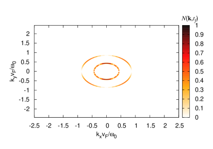
Figure 1: (Color online) Particle distribution function $N_{c}\left(\mathbf{k},t_{f}\right)$ (in arbitrary units) after the interaction at the instant $t_{f}=32\mathcal{T}$, as a function of scaled dimensionless momentum components. The wave is assumed to be linearly polarized with a dimensionless parameter $\chi_{0}=0.2$.

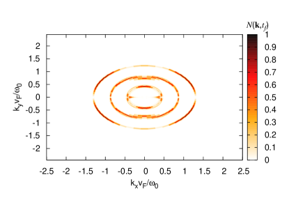
Figure 2: (Color online) Creation of a particle-hole pair in TI at multiphoton excitation. Particle distribution function $N_{c}\left(\mathbf{k},t_{f}\right)$ (in arbitrary units) after the interaction is displayed for a wave intensity $\chi_{0}=0.5$.

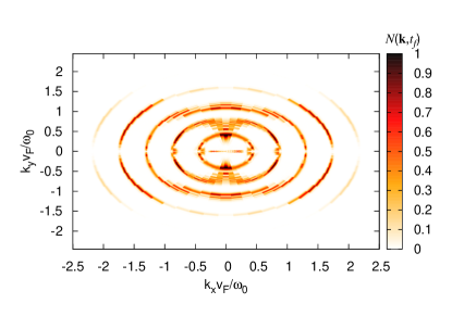
Figure 3: (Color online) The same as Fig. 2 but for $\chi_{0}=1$.

In Fig. 2 the creation of a particle-hole pair in TI is shown for stronger wave intensity $\chi_{0}=0.5$. With increasing pump wave intensity and approaching to the domain $\chi_{0}\sim 1$, the multiphoton excitations takes place and the Rabi oscillations appear corresponding to multiphoton transitions. At that, one should take into account the intensity effect of the pump wave (Stark shift due to free-free intraband transitions) and Coulomb effect on the quasienergy spectrum. Thus, the multiphoton probabilities of particle-hole pair production have maximal values for the resonant transitions

$$\overline{\omega}\left(\mathbf{k}_{0}\right)=n\hbar\omega_{0},\ \ n=1,2,3...,$$ (31)

where

$$\overline{\omega}\left(\mathbf{k}_{0}\right)=\frac{1}{\mathcal{T}}\int\limits_{0}^{\mathcal{T}}\left(\omega\left(\mathbf{k}_{0}+\mathbf{k}_{E}\left(t\right)\right)+\omega_{\mathrm{PN}}\left(\mathbf{k}_{0}+\mathbf{k}_{E}\left(t\right),t\right)\right)dt$$ (32)

is the mean value of the Coulomb and wave-fields dressed transition frequency. For the effective high-harmonic generation multiphoton transitions (31) should have reasonable probabilities, that is, the generalized Rabi frequency and interaction time should be large enough for full Rabi flopping. As is seen from Fig. 3 at $\chi_{0}=1$, the probabilities of multiphoton transitions are considerable up to photon numbers $s=5$. With the multiphoton excitation the total electronic density

$$n_{c}\left(t\right)=\int N_{c}\left(\mathbf{k},t\right)\frac{d\mathbf{k}}{\left(2\pi\right)^{2}}$$ (33)

is also varied, approaching to a maximal value, and then falling. The latter is plotted in Fig. 4. Here $n_{0}=\omega_{0}^{2}/\left(2\pi\mathrm{v}_{F}^{2}\right)$ and for a THz photon $n_{0}=1.43\times 10^{9}\mathrm{cm}^{-2}$.

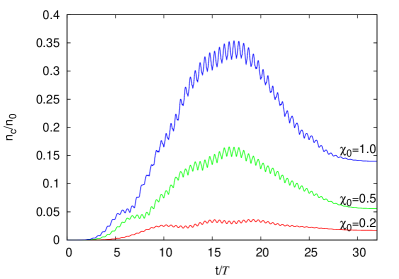
Figure 4: (Color online) Time evolution of the total normalized electronic density (in arbitrary units) at various pump wave intensities.

At the multiphoton excitation, the particle-hole annihilation and the intraband transitions will cause intense coherent radiation of the harmonics of the applied wave field. Here we consider the possibility of generation of harmonics at the multiphoton excitation depending on the pump field intensity and frequency. For the radiation spectrum, one needs the mean value of the current density operator

$$\widehat{\mathbf{j}}=-e\langle\ \widehat{\Psi}|\widehat{\mathbf{v}}|\ \widehat{\Psi}\rangle,$$ (34)

where $\widehat{\mathbf{v}}=\hbar^{-1}\partial H_{0}\left(\mathbf{k}\right)/\partial\mathbf{k}$ is the velocity operator. Here we need only the surface current in the polarization direction of the pump wave: $\mathcal{J}_{x}\left(t\right)=\left\langle\widehat{j}_{x}\right\rangle/\mathcal{A}$. For the effective Hamiltonian (1) the x-component of the velocity operator reads

$$\widehat{\mathrm{v}}_{x}=\mathrm{v}_{F}\left(\begin{array}[]{cc}0&-i\\ i&0\end{array}\right).$$ (35)

With the help of Eqs. (7), (12), (34), and (35), the surface current can be written as

$$\mathcal{J}_{x}\left(t\right)=-\frac{e\mathrm{v}_{F}}{(2\pi)^{2}}\int d\mathbf{k}\left[\cos\theta(\mathbf{k})\left(N_{c}\left(\mathbf{k},t\right)-N_{v}\left(\mathbf{k},t\right)\right)\right.$$

$$\left.+2\sin\theta(\mathbf{k})P^{\prime\prime}\left(\mathbf{k},t\right)\right].$$ (36)

Thus, having solutions of Eqs. (15), (16), and (17), then making an integration in Eqs. (36) one can calculate the harmonic radiation spectrum with the help of a Fourier transform of the function $\mathcal{J}_{x}\left(t\right)$. We assume that the spectrum is measured at a fixed observation point in the backward propagation direction (and pump wavelength is much larger than TI film thickness). For the generated field we have

$$E_{x}^{(g)}\left(t+z/c\right)=-\frac{4\pi}{c}\mathcal{J}_{x}\left(t+z/c\right).$$ (37)

The emission strength of the $s$th harmonic will be characterized by the dimensionless parameter

$$\chi_{s}=\frac{eE_{x}^{(g)}\left(s\right)\mathrm{v}_{F}}{\hbar\omega_{0}^{2}}=\chi_{0}\frac{E_{x}^{(g)}\left(s\right)}{E_{0}},$$ (38)

where

$$E_{x}^{(g)}\left(s\right)=\frac{\omega_{0}}{2\pi}\int_{0}^{2\pi/\omega_{0}}E_{x}^{(g)}\left(t\right)e^{is\omega_{0}t}dt$$ (39)

is the Fourier component of the generated field. In Fig. 5 the density plot of the radiation spectrum via logarithm of the normalized field strength $\chi\left(\omega\right)$ (in arbitrary units) versus the pump wave intensity is illustrated. Note that with the fast Fourier transform algorithm instead of discrete functions $\chi_{s}$ we calculate smooth function$\chi\left(\omega\right)$ and so $\chi_{s}=\chi\left(s\omega_{0}\right)$. From this figure, we clearly notice maximums at the odd harmonics and with the increase of the wave intensity the emission strengths of the high harmonics become feasible and for $\chi_{0}=2$ harmonics up to 21th are sizable.

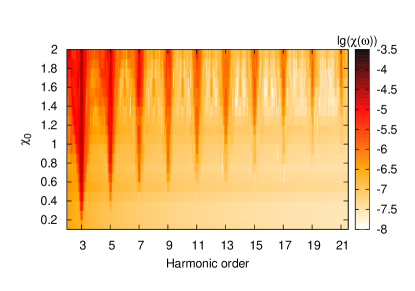
Figure 5: (Color online) Density plot of the radiation spectrum via logarithm of the normalized field strength $\chi\left(\omega\right)$ (in arbitrary units) versus the pump wave intensity. The wave frequency is taken to be $\nu_{0}=1\ \mathrm{THz}$.

We further examine emission rates of the 3rd and 5th harmonics for various pump wave frequencies versus intensity, which are shown in Figs. 6 and 7. For the considered intensities the perturbation theory is not applicable and in Figs. 6 and 7 we have a strong deviation from power law for the emission rates of harmonics. In particular, the rate of the 3rd harmonic scales is almost linearly on the pump wave strength $\chi_{3}\sim\chi_{0}$. Whereas it should show the $\chi_{0}^{3}$ dependence in the perturbative limit. Besides, these figures show that the emission rates almost independent of the pump wave frequency.

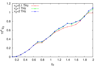
Figure 6: (Color online) Third harmonic emission rate in TI versus pump wave intensity for various wave frequencies.

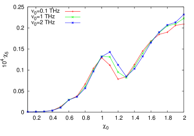
Figure 7: (Color online) Fifth harmonic emission rate in TI versus pump wave intensity for various wave frequencies.

Thus, calculations show that at the multiphoton excitation of 2D metallic surface states of TI the generation of high harmonics is possible which takes place for the wide range of pump wave frequencies. The average intensity of the wave expressed by $\chi_{0}$, can be estimated as

$$I_{\chi_{0}}=\chi_{0}^{2}\times 2\times 10^{2}\ \mathrm{W\ cm}^{-2}\left(\frac{\nu_{0}}{\mathrm{THz}}\right)^{4}.$$ (40)

The intensity $I_{\chi_{0}}$ strongly depends on the pump wave frequency. In particular for THz pump waves, high-harmonics can be generated at the intensities $I_{\chi_{0}\approx 1}\approx 2\times 10^{2}\ \mathrm{W\ cm}^{-2}$.

4 Conclusion

We have presented a nonlinear microscopic theory of the TI interaction with coherent electromagnetic radiation in the ultrafast excitation regime. Electron-electron Coulomb interaction has been taken into account with the self-consistent Hartree-Fock approximation that leads to a closed set of integrodifferential equations for the interband polarization and carrier occupation distribution. The dynamics of the multiphoton excitation of 2D metallic surface states of TI depending on the wave intensity has been considered and analyzed on the basis of numerical simulations. It has been shown that by THz radiation of moderate intensities, one can control interband multiphoton transitions in 2D metallic surface states of TI on time scales $t\lesssim 100\ \mathrm{ps}$. Furthermore, we have shown that along with multiphoton transitions there is an intense radiation of high harmonics at the interband (particle-hole annihilation) and intraband transitions induced by a pump wave. The obtained results certify that the process of high-harmonic generation for THz photons can be already observed for intensities $\sim 0.2\ \mathrm{kW\ cm}^{-2}$ and temperatures $T<<$ $\hbar\omega_{0}$.

This work was supported by the RA MES State Committee of Science and Belarusian Republican Foundation for Fundamental Research (RB) in the frames of the joint research projects SCS AB16-19 and BRFFR F17ARM-25, accordingly.

References

References

• [1] Hasan M Z, Kane C L 2010 Rev. Mod. Phys. 82 3045
• [2] Qi X L, Zhang S C 2011 Rev. Mod. Phys. 83 1057
• [3] Hsieh D, Xia Y, Qian D, Wray L, Meier F, Dil J H, Osterwalder J, Patthey L, Fedorov AV, Lin H, Bansil A Phys. Rev. Lett. 2009 103 146401
• [4] Zhang T, Cheng P, Chen X, Jia J F, Ma X, He K, Wang L, Zhang H, Dai X, Fang Z, Xie X 2009 Phys. Rev. Lett. 103 266803
• [5] Tse W K, Macdonald A H 2010 Phys. Rev. Lett. 105 057401
• [6] Tse W K, Macdonald A H 2010 Phys. Rev. B 82 161104
• [7] Hosur P 2011 Phys. Rev. B 83 035309
• [8] Iurov A, Gumbs G, Roslyak O, Huang D 2013 J. Phys.: Condens. Matter 25 135502
• [9] Rahim K, Ullah A, Tahir M, Sabeeh K 2017 J. Phys.: Condens. Matter 29 425304
• [10] Jenkins G S, Sushkov A B, Schmadel D C, Butch N P, Syers P, Paglione J, Drew H D 2010 Phys. Rev. B 82 125120
• [11] Sushkov A B, Jenkins G S, Schmadel D C, Butch N P, Paglione J, Drew H D 2010 Phys. Rev. B 82 125110
• [12] Hsieh D, McIver J W, Torchinsky D H, Gardner D R, Lee Y S, Gedik N 2011 Phys. Rev. Lett. 106 057401
• [13] Peres N M R, Santos J E 2013 J. Phys.: Condens. Matter 25 305801
• [14] Autore M, Di Pietro P, Di Gaspare A, D’Apuzzo F, Giorgianni F, Brahlek M, Koirala N, Oh S, Lupi S 2017 J. Phys.: Condens. Matter 29 183002
• [15] Giorgianni F, Chiadroni E, Rovere A, Cestelli-Guidi M, Perucchi A, Bellaveglia M, Castellano M, Di Giovenale D, Di Pirro G, Ferrario M, Pompili R 2016 Nat. Commun. 7 11421
• [16] Mikhailov S A, Ziegler K 2008 J. Phys.: Condens. Matter 20 384204
• [17] Avetissian H K, Avetissian A K, Mkrtchian G F, Sedrakian Kh V 2012 Phys. Rev. B 85 115443
• [18] Avetissian H K, Avetissian A K, Mkrtchian G F, Sedrakian Kh V 2012 J. Nanophoton. 6, 061702
• [19] Avetissian H K, Ghazaryan A G, Mkrtchian G F, Sedrakian Kh V 2017 J. Nanophoton. 11 016004
• [20] Yoshikawa N, Tamaya T, Tanaka K 2017 Science 356 736
• [21] Abergel D S L, Das Sarma S 2013 Phys. Rev. B 87 041407
• [22] Das Sarma S, Li Q 2013 Phys. Rev. B 88 081404
• [23] Viljas J K, Heikkilä T T 2010 Phys. Rev. B 81, 245404