Entropy production and fluctuations in a Maxwell’s refrigerator with squeezing

Abstract

Clarifying the impact of quantumness in the operation and properties of thermal machines represents a major challenge. Here we envisage a toy model acting either as an information-driven fridge or as heat-powered information eraser in which coherences can be naturally introduced in by means of squeezed thermal reservoirs. We study the validity of the transient entropy production fluctuation theorem in the model with and without squeezing as well as its decomposition into adiabatic and non-adiabatic contributions. Squeezing modifies fluctuations and introduces extra mechanisms of entropy exchange. This leads to enhancements in the cooling performance of the refrigerator, and challenging Landauer’s bound in the setup.

I Introduction

In 1871 Maxwell proposed his famous thought experiment illustrating the deep link between information and thermodynamics, today known as Maxwell’s demon Plenio ; Mayurama ; ParrondoInfo . In the though experiment, a little intelligent being acquires information about the positions and velocities of the molecules of two gases at different temperatures. The gases are separated by a rigid wall in containers of equal volume, and the demon can control a tiny door in the wall which can be open or closed, letting fast (hot) particles of the cold temperature container pass to the hot temperature container when they approach the wall. This may result in a paradoxical heat current against a temperature gradient without any invested work, a situation which challenges the second law of thermodynamics.

Nowadays it is well understood that information modifies the energetic restrictions imposed by the second law Plenio ; Mayurama ; ParrondoInfo , as anticipated by Leo Szilard in 1929 Szilard . One of the most popular solutions to Maxwell’s demon paradox is due to Charles Bennett Bennett , who invoked Landauer’s erasure principle Landauer . Following Landauer, logical erasure of a bit of information in a system in contact with a thermal reservoir at temperature $T$ requires a minimum dissipation of heat, $Q_{\mathrm{eras}}\geq k_{B}T\ln 2$, which is called Landauer’s bound. Landauer’s principle has been experimentally verified at the single particle level both in classical Berut and quantum systems Peterson . Moreover, both classical and quantum devices acting as Maxwell’s demon have been recently proposed Mandal ; MandalII ; Strasberg ; Chapman ; Elouard and implemented in the laboratory in a variety of physical systems Toyabe ; Koski ; Roldan ; KoskiII ; Photonic ; Camati ; Cottet .

A major challenge in quantum thermodynamics PaulReview ; AndersReview is to determine the impact of genuinely quantum effects in the thermodynamic behavior and properties of small systems subjected to fluctuations. This is specially interesting in the case of non-ideal environments, such as finite EspositoCorrelations ; Averin ; Reeb ; Suomela or non-thermal reservoirs Vaccaro ; LutzNeqR ; Alicki ; EspositoPRX . In particular, quantum coherence, squeezing and quantum correlations have been shown to improve the ability to extract work and the performance of quantum thermal machines Scully ; LutzCorrelations ; Li ; LutzSqueez ; Correa ; Hardal ; SqzRes ; Niedenzu ; Segal . However, unveiling the mechanisms responsible of such improvements and bounding their effects represents an open problem, which requires a precise formulation of the second law of thermodynamics in such non-equilibrium situations SqzRes ; Segal . In this context, the development of fluctuation theorems in the quantum regime CampisiFTReview ; EspositoFTReview has provided useful tools to understand the deep relation between dissipation and irreversibility. Indeed fluctuation theorems have been very recently extended to the case of a quantum system coupled to non-ideal reservoirs and following arbitrary quantum evolutions New (see also Ref. MHP ). These new extensions can help to unveil the thermodynamic properties of small thermal machines operating with non-thermal quantum reservoirs, being the squeezed thermal reservoir one of the most paradigmatic examples.

Squeezing constitutes a useful resource not only from the perspective of quantum information, with applications in quantum metrology, imaging, computation, and cryptography Polzik:2008 , but also from the perspective of quantum thermodynamics, as its presence in an otherwise thermal reservoir introduces modifications in the second law SqzRes . The defining feature of squeezing is the introduction of asymmetry between the position and momentum uncertainties Ficek . This allows squeezed thermal states to support higher energies for the same value of the entropy than Gibbs thermal states, and induces important modifications in the energy fluctuations Fearn ; Kim . Squeezed thermal states were first implemented in the lab for light at microwave frequencies Yurke , while nowadays they can be implemented even in massive high-frequency mechanical oscillators Wollman ; Pirkkalainen ; Rashid . A proposal for mimicking a squeezed thermal reservoir in a quantum heat engine configuration has been presented for an ion trap configuration LutzSqueez ; LutzAtom . Furthermore, a recent experiment has shown the operation of a nanobeam heat engine coupled to a squeezed thermal reservoir, where enhancements over Carnot efficiency has been experimentally checked Klaers .

In this article, we analyze the impact of reservoir squeezing in the fluctuations and thermodynamics of a quantum device acting either as an information power fridge (Maxwell’s refrigerator) or as a heat driven information eraser (Landauer’s eraser). A classical model of an autonomous device showing these two regimes has been proposed in Ref. Mandal , and extended to the quantum regime in Ref. Chapman . We propose a different model which is reminiscent of the Büttiker-Landauer ratchet Buttiker ; Landauer-But . Here the exchange of heat between reservoirs at different temperatures are controlled by a semi-infinite energyless memory system. Our approach consist in analyzing the dynamical evolution of this system within the framework of quantum trajectories. This allows us to apply recent results in quantum fluctuation theorems MHP ; New to the present configuration, which in turn provides a precise statement of the second law of thermodynamics in the setup. Comparing the cases in which reservoirs are purely thermal and thermal squeezed, we then obtain explicit expressions for the enhancements in the device performance, illustrating how Landauer’s principle is modified by means of environmental squeezing.

II Setup

Consider a small thermal device acting between two resonant bosonic reservoirs at different (inverse) temperatures $\beta_{r}=1/k_{B}T_{r}$, and an external memory system, $M$, in which information can be erased or stored when it is put in contact with the device (see Fig. 1). The memory is considered here to be a semi-infinite set of quantum levels $\{\ket{0},\ket{1},...,\ket{n},...\}$ with degenerate energies (conveniently set to zero), and ladder operators $[a_{L}^{~{}},a_{L}^{\dagger}]=\mathbb{I}$, producing jumps between the degenerate levels to the left ($a_{L}$) or to the right ($a_{R}\equiv a_{L}^{\dagger}$). The memory $M$ and the reservoir modes weakly couple throughout a three-body interaction term:

$$H_{I}=\hbar g\left(a_{L}b^{\dagger}c+a_{R}bc^{\dagger}\right),$$ (1)

where $g\ll\omega$, being $\omega$ the natural frequency of the reservoir modes, $H_{1}=\hbar\omega b^{\dagger}b$ and $H_{2}=\hbar\omega c^{\dagger}c$, and where $[b,b^{\dagger}]=\mathbb{I}$ $([c,c^{\dagger}]=\mathbb{I})$ are the ladder operators of the two reservoir bosonic modes. The above interaction Hamiltonian preserves energy and induces jumps on the memory to the left (right) when an energy quantum is transferred from the reservoir $2$ ($1$) to the reservoir $1$ ($2$). The underlying idea of the model is to profit from environment induced heat flows throughout the device modes in order to push the state of the memory as much as possible to its leftmost level $\ket{0}$ (Landauer’s erasure), or alternatively, use the memory in order to induce the desired heat flows between the reservoir against constrains imposed by the environment (Maxwell’s refrigerator).

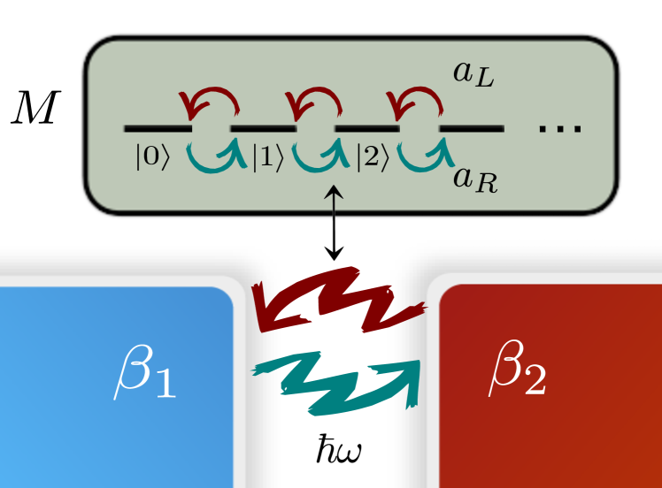
Figure 1: Schematic diagram of the setup. Two reservoirs of resonant bosonic modes at different (inverse) temperatures $\beta_{1}\geq\beta_{2}$ are able to exchange energy by inducing jumps between the degenerate energy levels of the external memory (M). Each time a quantum $\hbar\omega$ of heat is transferred from the hot (cold) to the cold (hot) reservoirs, the memory performs a collective jump to the left (right) as given by the operator $a_{L}$ ($a_{R}$).

We first consider the case in which both reservoirs are ideal thermal reservoirs in equilibrium at temperatures $\beta_{1}\geq\beta_{2}$. This means that the environmental bosonic modes are assumed to be always in a Gibbs state. We are interested in the relaxation dynamics of this model when starting from an arbitrary initial state in the memory. Using standard techniques form open quantum system theory BreuerBook , one arrives to the following master equation for the dissipative dynamics of the memory density operator, $\rho_{t}$:

$$\dot{\rho}_{t}=\mathcal{L}(\rho_{t})= \Gamma_{\leftarrow}\left(a_{L}\rho_{t}a_{R}-\frac{1}{2}\{a_{R}a_{L},\rho_{t}\}\right)$$

$$+\Gamma_{\rightarrow}\left(a_{R}\rho_{t}a_{L}-\frac{1}{2}\{a_{L}a_{R},\rho_{t}\}\right),$$ (2)

where we neglected Lamb-Stark frequency shifts. The above equation can be straightforwardly checked to be in Lindblad form Lindblad by identifying the (two) Lindblad operators $L_{\leftarrow}=\sqrt{\Gamma_{\leftarrow}}~{}a_{L}$ and $L_{\rightarrow}=\sqrt{\Gamma_{\rightarrow}}~{}a_{R}$. Equation (II) describes incoherent jump processes in the memory to the left at rate $\Gamma_{\leftarrow}=\gamma(n_{1}^{\rm th}+1)n_{2}^{\rm th}$, and to the right at rate $\Gamma_{\rightarrow}=\gamma(n_{2}^{\rm th}+1)n_{1}^{\rm th}$, $\gamma$ being a constant depending on the interaction strength and $n_{r}^{\rm th}\equiv(e^{\beta_{r}\hbar\omega}-1)^{-1}$. Contact with the thermal reservoirs implies a detailed balance relation between jumps

$$\Gamma_{\leftarrow}=e^{\mu}\Gamma_{\rightarrow},~{}~{}~{}~{}\mathrm{where}~{}~{}~{}\mu\equiv(\beta_{1}-\beta_{2})\hbar\omega\geq 0.$$ (3)

In the long-time run, the memory system reaches a steady state where jumps to the left and to the right becomes equally probable. This steady state can be obtained from the master equation (II) by setting $\mathcal{L}(\pi)=0$. We obtain

$$\pi=\frac{e^{-\mu N_{M}}}{Z},$$ (4)

where $N_{M}=a_{L}^{\dagger}a_{L}^{~{}}$ is the number operator in the memory, and $Z=\mathrm{Tr}[\exp(-\mu N_{M})]=(1-e^{-\mu})^{-1}$. The quantity $\mu$ fully determines the steady-state occupation in the degenerate energy levels of the memory, together with its entropy $S(\pi)=\mu\braket{N_{M}}_{\pi}+\ln Z$, being $\braket{N_{M}}_{\pi}=(e^{\mu}-1)^{-1}$. Consequently, the greater the temperature gradient between the reservoirs, the greater $\mu$, the more peaked the distribution in the level leftmost, and the lower the entropy of the steady state. On the contrary, if the temperatures of the reservoirs are very similar $\beta_{1}\rightarrow\beta_{2}$, we have $\mu\rightarrow 0$, and the steady state of the external system approaches the fully mixed state.

Notice that this simple toy model has all the necessary elements to act as Maxwell’s demon, where the heat flows are connected to the informational state of the memory system (regardless of its energy). On the one hand, if the initial state of the memory is a low entropic state (in particular if it has lower entropy than $\pi$), we can think about it as an information battery powering a flux of heat against the temperature gradient introduced by the reservoirs. This flow is maintained until the memory reaches the steady state $\pi$, and has hence to be replaced. On the other hand, if the initial state is very mixed (if it has greater entropy than $\pi$), we can think in our device as a Landauer’s eraser, which profits from the spontaneous heat flow from the hot to the cold reservoirs to purify the memory state Mandal . This is an eraser in the sense that whatever the initial state of the memory, the device transforms it into a known ready-to-operate state $\pi$ (which ideally corresponds to an error-free pure state $\ket{0}$), hence erasing any information previously encoded on it.

III Quantum trajectories

We now focus on a stochastic thermodynamical description of the model by using the quantum jump approach JordanPRA ; JordanParrondo ; Pekola ; Liu ; Liu2 ; Suomela-ad ; CampisiHE ; Galperin ; MHP . Within this approach, the dynamics described by the master equation (II) can be unraveled to construct quantum trajectories $\gamma$ which are sampled according with some probabilities $P(\gamma)$ when the environment is monitored Wiseman . We start by expanding the dynamics in an infinite set of infinitesimal time evolution steps:

$$\rho_{t+dt}=\left(\mathbb{I}+dt\mathcal{L}\right)\rho_{t}\equiv{\mathcal{E}}(\rho_{t}),$$ (5)

where $\mathcal{L}$ is given in Eq. (II), and ${\mathcal{E}}(\rho_{t})=\sum_{k}{M}_{k}\rho_{t}{M}_{k}^{\dagger}$ is a CPTP map fulfilling $\sum_{k}M_{k}^{\dagger}M_{k}=\mathbb{I}$. Here the set $\{M_{k}\}$ with $k=\{0,\leftarrow,\rightarrow\}$ are the Kraus operators of the map. They introduce an interpretation of the dynamics as different random operations ${\mathcal{E}}_{k}(\rho_{t})\equiv M_{k}\rho_{t}M_{k}^{\dagger}$ occurring with probability $p_{k}=\mathrm{Tr}[M_{k}^{\dagger}M_{k}\rho_{t}]$. We have

$$M_{0} \equiv~{}\mathbb{I}-\frac{1}{2}\left(\Gamma_{\leftarrow}a_{L}^{\dagger}a_{L}+\Gamma_{\rightarrow}a_{R}^{\dagger}a_{R}\right),$$ (6)

$$M_{\leftarrow} \equiv\sqrt{dt}L_{\leftarrow}=\sqrt{dt~{}\Gamma_{\leftarrow}}~{}a_{L},$$ (7)

$$M_{\rightarrow} \equiv\sqrt{dt}L_{\rightarrow}=\sqrt{dt~{}\Gamma_{\rightarrow}}~{}a_{R},$$ (8)

where we identified the single pair of Lindblad operators introduced before $\{L_{\leftarrow},L_{\rightarrow}\}$, and we notice that ${\mathcal{E}}(\pi)=\pi$.

From Eqs. (6)-(8), it follows that the dynamical evolution is mostly characterized by the operation corresponding to $M_{0}$, as it occurs with probability of order 1. In contrast, operations associated to $M_{\leftarrow}$ and $M_{\rightarrow}$ occur with probability $dt$, leading to abrupt jumps in the state of the system. Therefore, between consecutive jumps (e.g. occurring at $t$ and $t^{\prime}$) the evolution is smooth but nonunitary, as given by the effective evolution operator

$${U}_{\rm eff}(t^{\prime},t)=\exp\left[-\frac{i}{\hbar}H_{\rm eff}(t^{\prime}-t)\right],$$ (9)

$$H_{\rm eff}=\mathbb{I}-\frac{i\hbar}{2}\left(\Gamma_{\leftarrow}a_{L}^{\dagger}a_{L}+\Gamma_{\rightarrow}a_{R}^{\dagger}a_{R}\right).$$ (10)

This is the basis for an alternative description of the dynamics, the so-called direct jump unraveling of the master equation. Within this approach the memory system state no longer evolves according to Eqs. (5) or (II), but it is given by a stochastic differential equation (the stochastic Schrödinger equation) providing the state of the system conditioned on the observed outcomes Wiseman .

A trajectory $\gamma$ can then be specified as the result of the following forward process. We start with the system in some arbitrary initial state $\rho_{0}$ at $t=0$ and perform a projective measurement in the $\rho_{0}$ eigenbasis, selecting an eigenstate $\ket{\psi_{n}}$ with probability $p_{n}$. Then by monitoring of the environment, we record the set of different jumps $k_{j}$ and the times $t_{j}$ where they occurred. We finally introduce a second projective measurement on the system at time $t=\tau$, performed in the $\rho_{\tau}$ eigenbasis as given by the solution of the master equation (II). This leaves the system in some final state $\ket{\phi_{m}}$ with associated eigenvalue $p_{m}^{\ast}$. A trajectory with $N$ jumps can then be represented by the set $\gamma=\{n,(k_{1},t_{1}),...,(k_{j},t_{j}),...,(k_{N},t_{N}),m\}$, where $n$ and $m$ are the outcomes of the initial and final projective measurements JordanParrondo ; New . The probability of such a trajectory is given by

$$P(\gamma)= \mathrm{Tr}[\Pi_{m}^{\ast}\mathcal{U}_{\tau,t_{N}}{\mathcal{E}}_{k_{N}}\mathcal{U}_{t_{N},t_{N-1}}...~{}{\mathcal{E}}_{k_{l}}~{}$$

$$~{}~{}~{}~{}~{}...~{}\mathcal{U}_{t_{2},t_{1}}{\mathcal{E}}_{k_{1}}\mathcal{U}_{t_{1},0}(\Pi_{n}\rho_{0}\Pi_{n})],~{}~{}~{}~{}$$ (11)

with $\mathcal{U}_{t_{j+1},t_{j}}(\rho)={U}_{\rm eff}(t_{j+1},t_{j})\rho\,{U}^{\dagger}_{\rm eff}(t_{j+1},t_{j})$ and where for simplicity we considered initial and final rank-1 projectors $\Pi_{n}\equiv\ket{\psi_{n}}\bra{\psi_{n}}$ and $\Pi_{m}^{\ast}\equiv\ket{\phi_{m}}\bra{\phi_{m}}$ respectively.

III.1 Backward process and total entropy production

Trajectories $\gamma$ can be associated to twin trajectories in which the sequence of events have been inverted, $\tilde{\gamma}=\{m,(k_{N},t_{N}),...,(k_{j},t_{j}),...,(k_{1},t_{1}),n\}$, sampled from the time-reversed process. This includes changing the order of initial and final projective measurements, and considering a backward dynamics corresponding to the evolution generated from time-inversion of the global dynamics in system and environment JordanParrondo ; New . This backward dynamics can be characterized by a concatenation of CPTP maps $\tilde{{\mathcal{E}}}$ in analogy to Eq. (5). We call $\tilde{{\mathcal{E}}}$ the backward map, which is equipped with a set of Kraus operators $\{\tilde{M}_{k}\}$ fulfilling New

$$\tilde{M}_{k}=e^{-\sigma_{k}^{E}/2}~{}\Theta M_{k}^{\dagger}\Theta^{\dagger}~{}~{}~{}\forall k,$$ (12)

where $\Theta$ is the time-reversal operator in quantum mechanics, and the set $\{\sigma_{k}^{E}\}$ are the stochastic entropy changes in the environment associated to any operation $k$. This guarantees the validity of the detailed and integral fluctuation theorems for the total entropy production

$$\frac{P(\gamma)}{\tilde{P}(\tilde{\gamma})}=e^{\Delta_{\mathrm{i}}s_{\mathrm{tot}}(\gamma)},~{}~{}~{}~{}\langle e^{-\Delta_{\mathrm{i}}s_{\mathrm{tot}}}\rangle_{\gamma}=1,$$ (13)

$\langle A\rangle_{\gamma}$ denoting the average of quantity $A(\gamma)$ over all trajectories $\gamma$. Here the total entropy production at the trajectory level is given by New

$$\Delta_{\mathrm{i}}s_{\mathrm{tot}}(\gamma)\equiv\Delta s_{m,n}+\sum_{j\in\gamma}\sigma^{E}_{k_{j}},$$ (14)

consisting in two terms. The first one, $\Delta s_{mn}\equiv-\ln p_{m}^{\ast}+\ln p_{n}$, is the stochastic entropy change in the memory system Seifert ; Sagawa ; JordanPRA , whose average yields the corresponding change in von Neumann entropy $\langle\Delta s_{mn}\rangle_{\gamma}=S(\rho_{\tau})-S(\rho_{0})$, with $S(\rho)=-\mathrm{Tr}[\rho\ln\rho]$. The second one is the collection of environmental entropy changes $\{\sigma_{k_{j}}^{E}\}$ due to the different jumps $k_{j}$ during the trajectory $\gamma$.

Furthermore, in Eq. (13) we introduced $\tilde{P}(\tilde{\gamma})$ as the probability of obtaining trajectory $\tilde{\gamma}$ in the backward process. It reads

$$\tilde{P}(\tilde{\gamma})= \mathrm{Tr}[\Theta\Pi_{n}\Theta^{\dagger}~{}\tilde{\mathcal{U}}_{t_{1},0}\tilde{{\mathcal{E}}}_{k_{1}}\tilde{\mathcal{U}}_{t_{2},t_{1}}~{}...~{}\tilde{{\mathcal{E}}}_{k_{l}}~{}$$

$$~{}~{}~{}~{}~{}...~{}\tilde{\mathcal{U}}_{t_{N},t_{N-1}}\tilde{{\mathcal{E}}}_{k_{N}}\tilde{\mathcal{U}}_{\tau,t_{N}}(\Theta\Pi_{m}^{\ast}\rho_{\tau}\Pi_{m}^{\ast}\Theta^{\dagger})],$$ (15)

where $\tilde{{\mathcal{E}}}_{k}(\rho)=\tilde{M}_{k}\rho\tilde{M}_{k}^{\dagger}$ are the backward operations associated to the Kraus operators in Eq. (12), and $\tilde{\mathcal{U}}_{t^{\prime},t}(\rho)=\tilde{U}_{\mathrm{eff}}(t^{\prime},t)\rho\tilde{U}_{\mathrm{eff}}^{\dagger}(t^{\prime},t)$ represents again a nonunitary smooth evolution

$$\tilde{U}_{\rm eff}(t^{\prime},t)=\exp\left[\frac{i}{\hbar}\Theta H_{\rm eff}^{\dagger}\Theta^{\dagger}(t^{\prime}-t)\right],$$ (16)

where $H_{\mathrm{eff}}$ is the same as in Eq. (9).

Following Ref. New , for systems with paired Lindblad operators $\{L_{k},L_{k^{\prime}}\}$ such that $L_{k}=\sqrt{\Gamma_{k}}L$, $L_{k}=\sqrt{\Gamma_{k^{\prime}}}L^{\dagger}$ for some $L$ (as it is the case here), one necessarily has $\sigma_{0}^{E}=0$ and $\sigma_{k}^{E}=\ln(\Gamma_{k}/\Gamma_{k^{\prime}})=-\sigma_{k^{\prime}}^{E}$. Therefore, we obtain the following stochastic entropy changes in the reservoirs associated to each Kraus operator in Eqs. (6)-(8)

$$\sigma_{0}^{E}=0,~{}~{}~{}~{}~{}\sigma_{\leftarrow}^{E}=\mu,~{}~{}~{}~{}~{}\sigma_{\rightarrow}^{E}=-\mu.$$ (17)

When a jump to the left (right) occurs, the entropy in the environment increases (decreases) by $\mu=(\beta_{1}-\beta_{2})\hbar\omega~{}(-\mu)$, associated to the exchange of a quantum of energy $\hbar\omega$ from the hot (cold) to the cold (hot) reservoir. For the backward evolution we then have the operators [Eq. (12)]:

$$\tilde{M}_{0} =\Theta M_{0}^{\dagger}\Theta^{\dagger}=M_{0},$$ (18)

$$\tilde{M}_{\leftarrow} =\sqrt{dt}\tilde{L}_{\leftarrow}=\Theta\sqrt{dt}L_{\rightarrow}\Theta^{\dagger}=M_{\rightarrow},$$ (19)

$$\tilde{M}_{\rightarrow} =\sqrt{dt}\tilde{L}_{\rightarrow}=\Theta\sqrt{dt}L_{\leftarrow}\Theta^{\dagger}=M_{\leftarrow}.$$ (20)

We obtain that the forward and the backward maps are essentially equal, and operations corresponding to a jump to the left in the forward process transforms into a jump to the right in the backward process, and vice-versa.

III.2 Adiabatic and non-adiabatic entropy production

The fluctuation theorems for the total entropy production in Eq. (13) can be further complemented with independent fluctuation theorems for the so called adiabatic and non-adiabatic entropy productions EspositoFT ; JordanParrondo ; New . These two entropy productions appear when discussing the different sources of irreversibility in standard thermodynamic configurations EspositoFT ; EspositoFaces , leading to the split

$$\Delta_{\mathrm{i}}s_{\mathrm{tot}}(\gamma)=\Delta_{\mathrm{i}}s_{\mathrm{ad}}(\gamma)+\Delta_{\mathrm{i}}s_{\mathrm{na}}(\gamma).$$ (21)

On the one hand, $\Delta_{\mathrm{i}}s_{\mathrm{na}}(\gamma)$ represents the non-adiabatic entropy production, created whenever the state of the system $\rho_{t}$ is different from the steady state of the dynamics $\pi$. For time-dependent Hamiltonians, the average non-adiabatic entropy production $\langle\Delta_{\mathrm{i}}s_{\mathrm{na}}(\gamma)\rangle_{\gamma}$ typically vanishes for very slow (quasi-static) driving, since in this situation the state of the system follows the (time-dependent) steady state EspositoFT ; EspositoFaces ; New . On the other hand, $\Delta_{\mathrm{i}}s_{\mathrm{ad}}$ is the adiabatic entropy production, which appears when the dynamical evolution is driven by nonequilibrium external constrains. Indeed, the adiabatic entropy production becomes the only source of entropy production for the case in which the system reaches a non-equilibrium steady state.

In Ref. New fluctuation theorems for the adiabatic and non-adiabatic entropy production, as the one in Eq. (13), have been established for a broad class of quantum evolutions. They are based on the comparison of the forward process statistics $P(\gamma)$ with the ones in two accessory twin processes: the dual and dual-reverse processes, previously introduced in the context of stochastic thermodynamics SeifertReview ; EspositoFT . These two processes are related between them by inversion of time. That is, the dual process generates forward trajectories like $\gamma$, while in the dual-reverse process the sequence of events is inverted and, as a consequence, trajectories $\tilde{\gamma}$ are generated. However, in both cases the infinitesimal dynamics are defined by new maps, namely the dual ${\mathcal{D}}$ and dual-reverse maps $\tilde{{\mathcal{D}}}$. Their corresponding Kraus operations must fulfill New (see also Refs. Crooks ; MHP )

$$D_{k}=e^{-(\sigma^{E}_{k}+\Delta\phi_{k})/2}~{}M_{k},~{}~{}~{}~{}\tilde{D}_{k}=e^{\Delta\phi_{k}/2}~{}\Theta M_{k}^{\dagger}\Theta^{\dagger}.$$ (22)

Here we introduced the quantities $\Delta\phi_{k}$, representing the change in a very particular observable of the system associated to the operator $M_{k}$ of the forward process, the so-called nonequilibrium potential MHP

$$\Phi\equiv-\ln\pi=\sum_{i}\phi_{i}\ket{\pi_{i}}\bra{\pi_{i}},$$ (23)

$\ket{\pi_{i}}$ being the eigenstates of the steady state $\pi$. The nonequilibrium potential has long been used in classical irreversible thermodynamics with non-equilibrium steady states Hanggi ; Hatano and in the context of fluctuation-dissipation theorems Prost (see also Hanggi ). Sufficient conditions for Eqs. (22) to hold are New ; MHP

$$\tilde{{\mathcal{E}}}(\Theta\pi\Theta^{\dagger})=\Theta\pi\Theta^{\dagger},~{}~{}~{}~{}[\Phi,L_{k}]=\Delta\phi_{k}~{}L_{k},$$ (24)

when ${\mathcal{E}}(\pi)=\pi$ is a positive-definite state. All these conditions hold in the present case as we will shortly see.

The adiabatic and non-adiabatic entropy production contributions in Eq. (21) can be then defined by comparing the trajectory probabilities between the original and the dual and dual-reverse processes EspositoFT ; Seifert . They result New

$$\Delta_{\mathrm{i}}s_{\mathrm{na}}(\gamma)=\Delta s_{nm}-\sum_{j\in\gamma}\Delta\phi_{k_{j}},$$ (25)

$$\Delta_{\mathrm{i}}s_{\mathrm{ad}}(\gamma)=\sum_{j\in\gamma}\sigma_{k_{j}}^{E}-\sum_{j\in\gamma}\Delta\phi_{k_{j}},$$ (26)

which fulfill independent detailed and integral fluctuation theorems as the one in Eq. (13), provided the conditions in Eq. (24) are obeyed.

From the steady state (4), the nonequilibrium potential reads:

$${\Phi}=-\ln\pi=\mu N+\ln Z.$$ (27)

It is now easy to see that the Kraus operators in Eqs. (6)-(8) are related to a unique change in the nonequilibrium potential, that is, $[{\Phi},L_{k}]=\Delta\phi_{k}L_{k}$ for $k=\{\leftarrow,\rightarrow\}$, with associated potential changes

$$\Delta\phi_{0}=0,~{}~{}~{}~{}\Delta\phi_{\leftarrow}=-\mu,~{}~{}~{}~{}\Delta\phi_{\rightarrow}=\mu.$$ (28)

Furthermore, Eqs. (18)-(20) ensure that the map $\tilde{{\mathcal{E}}}$ has as invariant state $\tilde{\pi}=\Theta\pi\Theta^{\dagger}$.

Remarkably, by comparing Eqs. (17) and (28), we see that the changes in the nonequilibrium potential produced by the jumps exactly coincides with the decrease in stochastic entropy in the reservoirs, that is $\Delta\phi_{\leftarrow,\rightarrow}=-\sigma_{\leftarrow,\rightarrow}$. Therefore, we can conclude that in this case the dual-reverse and backward processes are exactly equal, and hence the dual process is just the original forward one, which implies zero adiabatic entropy production, $\Delta_{\mathrm{i}}s_{\mathrm{ad}}(\gamma)=0$. That is, the only contribution to the entropy production is non-adiabatic:

$$\Delta_{\rm i}s^{\rm na}_{\gamma} =\Delta_{\rm i}s_{\gamma}=\Delta s_{nm}-\sum_{j\in\gamma}\Delta\phi_{k_{j}}$$

$$\equiv\Delta s_{nm}-(\beta_{1}-\beta_{2})q_{\gamma},$$ (29)

and fulfills the detailed and integral fluctuation theorems in Eq. (13). In the last equality of Eq. (III.2) we identified the net heat, $q_{\gamma}$, flowing from the cold to the hot reservoir during the trajectory $q_{\gamma}=\hbar\omega(n_{\rightarrow}-n_{\leftarrow})$, where $n_{\rightarrow(\leftarrow)}$ is the total number of jumps right (left) detected during the trajectory $\gamma$. The absence of adiabatic entropy production can be understood from the fact that in this model, any transfer of heat between reservoirs is achieved by means of jumps in the memory, cf. Eq. (1). This implies that no heat can flow without modifying the system density operator, and hence no entropy can be produced irrespective of the changes in $\rho$, which is the defining feature of the non-adiabatic entropy production. As a consequence, any flow ceases in the long-time run, when the steady state $\pi$ is reached, blocking the heat transfer between the reservoirs.

III.3 Average entropy production rate

The integral fluctuation theorem in Eq. (13) has as an immediate corollary the positivity of the average entropy production $\langle\Delta_{\mathrm{i}}s_{\mathrm{tot}}\rangle\geq 0$. Furthermore, since the theorem can be applied to any infinitesimal instant of time, we immediately obtain the positivity of the total entropy production rate New

$$\dot{S}_{\mathrm{tot}}=\dot{S}-\dot{\sigma}^{E}\geq 0,$$ (30)

where $\dot{S}=-\mathrm{Tr}[\dot{\rho}_{t}\ln\rho_{t}]$ is the derivative of the von Neumann entropy of the system, and the entropy changes in the environment are given by $\dot{\sigma}^{E}dt=\sum_{k}\mathrm{Tr}[M_{k}^{\dagger}M_{k}\rho_{t}]\sigma_{k}^{E}$.

In this case we obtain:

$$\dot{S}_{\mathrm{tot}}=\dot{S}-\mu\braket{\dot{N}_{M}}=\dot{S}-(\beta_{1}-\beta_{2})\dot{Q}\geq 0,$$ (31)

where $\dot{Q}=\mathrm{Tr}[\dot{\rho}_{t}\hbar\omega N_{M}]$ is the heat flow from the cold to the hot reservoir. The second-law-like inequality (31), can be now used to illustrate the two different regimes of operations of the device. Indeed it put bounds on the performance of the two regimes of the device at any time of the dynamics, i.e. Landauer’s eraser and Maxwell’s refrigerator respectively. When $\dot{Q}<0$, that is, heat flows spontaneously from the hot to the cold reservoir, the entropy in the memory system is allowed to decrease, $\dot{S}<0$, until it compensates the entropy produced by the spontaneous heat flow. Following Eq. (31) The heat dissipated in the erasure process is lower bounded by

$$(\beta_{1}-\beta_{2})|\dot{Q}|\geq~{}|\dot{S}|,$$ (32)

which is a manifestation of Landauer’s principle in our setting. Here the quantity $\beta_{1}-\beta_{2}$ arises as an effective temperature of the memory system determining its steady state. On the other hand, if $\dot{S}>0$, now the flux of heat can be inverted against the thermal gradient, $\dot{Q}>0$ refrigerating the cold reservoir, at the price of entropy production in the memory system. The performance of the resulting Maxwell’s refrigerator can be analogously bounded

$$\dot{Q}~{}\leq~{}\frac{1}{\beta_{1}-\beta_{2}}\dot{S},$$ (33)

where $\dot{Q}$ is the relevant cooling rate, i.e. the amount of heat per unit time extracted from the cold reservoir.

IV Squeezed thermal reservoir enhancements

Once the thermodynamic behavior of the model has been analyzed for the case of ideal thermal reservoirs, we move to the case of non-canonical reservoirs. We replace both thermal reservoirs at inverse temperatures $\beta_{1}$ and $\beta_{2}$, by squeezed thermal reservoirs at the same temperatures, and additional complex parameters $\{\xi_{1},\xi_{2}\}$ characterizing the squeezing, where $\xi_{i}=r_{i}e^{i\theta_{i}}$ for $i=1,2$ Ficek ; BreuerBook .

The details on the dissipative dynamics induced by such a quantum reservoir in a bosonic mode, together with the analysis of its thermodynamic power have been reported in Ref. SqzRes . In the present situation we concern, the master equation in Eq. (II) changes to:

$$\dot{\rho}_{t}=\mathcal{L}^{\ast}(\rho_{t})= \Gamma_{-}\left(R~{}\rho_{t}R^{\dagger}-\frac{1}{2}\{R^{\dagger}R,\rho_{t}\}\right)$$

$$+\Gamma_{+}\left(R^{\dagger}\rho_{t}R-\frac{1}{2}\{RR^{\dagger},\rho_{t}\}\right),$$ (34)

where $R$ is the ladder operator of a Bogoliubov mode defined by the canonical transformation

$$R\equiv a_{L}\cosh(r)+a_{R}\sinh(r)~{}e^{i\theta}=\mathcal{S}(\xi)a_{L}\mathcal{S}^{\dagger}(\xi),$$ (35)

$\mathcal{S}(\xi)=\exp(\frac{r}{2}(a_{L}^{2}e^{-i\theta}-a_{R}^{2}e^{i\theta}))$ being the squeezing operator on the memory system. The complex parameter is $\xi=re^{i\theta}$, with $\theta\equiv\theta_{1}-\theta_{2}$, and $r\geq 0$. The later depends on all the reservoir temperatures and squeezing parameters through the relation

$$\tanh(2r)~{}\equiv\frac{2M_{1}M_{2}}{(N_{1}+1)N_{2}+(N_{2}+1)N_{1}},$$ (36)

where $M_{i}\equiv-\sinh(r_{i})\cosh(r_{i})(2n_{i}^{\rm th}+1)$ and $N_{i}\equiv n_{i}^{\rm th}\cosh(2r_{i})+\sinh(r_{i})$ for $i=1,2$. Notice that the above equation is only well defined for the right hand side taking values in between $0$ and $1$ (we recall that $r\geq 0$), to which we will restrict from now on. In addition we notice that $r\rightarrow 0$ when either $r_{1}\rightarrow 0$ or $r_{2}\rightarrow 0$.

The operators $R$ and $R^{\dagger}$ in the master equation (IV), promote jumps to the left and to the right, respectively, now between the states of the squeezed basis of the memory system: $\{\mathcal{S}\ket{0},\mathcal{S}\ket{1},...,\mathcal{S}\ket{n},...\}$. The rates of the jumps are given by

$$\Gamma_{\mp}=\frac{\gamma}{2}\left(\delta N\pm(N_{2}-N_{1})\right),$$ (37)

where $\delta N\equiv\sqrt{\left((N_{1}+1)N_{2}+(N_{2}+1)N_{1}\right)^{2}-4|M_{1}M_{2}|^{2}}$. Notice that the rates $\Gamma_{\mp}$ fulfill again a detailed balance relation for a new parameter $\Gamma_{-}=\Gamma_{+}~{}e^{\mu_{\ast}}$, where

$$\mu_{\ast}\equiv\ln\left(\frac{N_{1}\sinh^{2}(r)+N_{2}\cosh^{2}(r)+N_{1}N_{2}}{N_{1}\cosh^{2}(r)+N_{2}\sinh^{2}(r)+N_{1}N_{2}}\right),$$ (38)

which can be both greater or lower than $\mu$ depending on $\{r_{1},r_{2}\}$ (inside the allowed range). In particular, $\mu_{\ast}\rightarrow\mu$ only when both $r_{1}\rightarrow 0$ and $r_{2}\rightarrow 0$.

Crucially, the master equation (IV) now induces the following steady state reminiscent of the squeezed thermal state

$$\pi_{\ast}=\mathcal{S}(\xi)~{}\frac{e^{-\mu_{\ast}N_{M}}}{Z_{\ast}}~{}\mathcal{S}^{\dagger}(\xi),$$ (39)

with $\mu_{\ast}$ defined in Eq. (38), and $Z_{\ast}=\mathrm{Tr}[e^{-\mu_{\ast}N_{M}}]=(1-e^{-\mu_{\ast}})^{-1}$.

Following the trajectory formalism, the Kraus operators for the map ${\mathcal{E}}$ now reads

$$M_{0}=\mathbb{I}-\frac{1}{2}\left(\Gamma_{-}R^{\dagger}R+\Gamma_{+}RR^{\dagger}\right),$$ (40)

$$M_{-}=\sqrt{dt}L_{-}=\sqrt{dt~{}\Gamma_{-}}~{}R,$$ (41)

$$M_{+}=\sqrt{dt}L_{+}=\sqrt{dt~{}\Gamma_{+}}~{}R^{\dagger}.$$ (42)

with the new Lindblad operators, $\{L_{-},L_{+}\}$, again suitable to obtain the stochastic entropy changes in the reservoirs

$$\sigma_{0}^{E}=0,~{}~{}~{}~{}~{}\sigma_{-}^{E}=\mu_{\ast},~{}~{}~{}~{}~{}\sigma_{+}^{E}=-\mu_{\ast}.$$ (43)

Notice that the entropy changes in the environment $\sigma_{\mp}^{E}$, associated to the jumps have no longer a clear interpretation in terms of the exchange of an energy quantum between the reservoirs, as in this case both energy and coherence are exchanged between the reservoirs in each jump, producing (or annihilating) an entropy quantum $\pm\mu_{\ast}$ in the whole environment. Nevertheless the fluctuation theorems in Eq. (13) hold, and the Kraus operators for the backward map still fulfill the same structure than in the previous case

$$\tilde{M}_{0} =\Theta M_{0}^{\dagger}\Theta^{\dagger}=M_{0},$$ (44)

$$\tilde{M}_{-} =\sqrt{dt}\tilde{L}_{-}=\Theta\sqrt{dt}L_{+}\Theta^{\dagger}=M_{+},$$ (45)

$$\tilde{M}_{+} =\sqrt{dt}\tilde{L}_{+}=\Theta\sqrt{dt}L_{-}\Theta^{\dagger}=M_{-}.$$ (46)

The conditions (24) for the adiabatic and non-adiabatic decomposition of the total entropy production also hold in this case. Indeed, from the steady state (39) the nonequilibrium potential now reads

$${\Phi}=-\ln\pi_{\ast}=\mu_{\ast}\mathcal{S}N_{M}\mathcal{S}^{\dagger}+\ln Z_{\ast},$$ (47)

which fulfills $[{\Phi},L_{k}]=\Delta\phi_{k}L_{k}$ for $k=\{-,+\}$, being

$$\Delta\phi_{0}=0,~{}~{}~{}~{}\Delta\phi_{-}=-\mu_{\ast},~{}~{}~{}~{}\Delta\phi_{+}=\mu_{\ast}.$$ (48)

Moreover, the map $\tilde{{\mathcal{E}}}$ has as invariant state $\tilde{\pi}_{\ast}=\Theta\pi_{\ast}\Theta^{\dagger}$ as is required.

From Eqs. (43) and (48) we see that also in this case the changes in the nonequilibrium potential produced by the jumps exactly coincides with the decrease of stochastic entropy in the reservoirs, $\Delta\phi_{\mp}=-\sigma_{\mp}^{E}$. Hence the adiabatic entropy production remains zero in the squeezed thermal reservoirs case. This means that when the steady state $\pi_{\ast}$ is reached, no further entropy production is needed in order to maintain it. The average entropy production rate reads in this case

$$\dot{S}_{\rm tot} =\dot{S}-\mu_{\ast}\mathrm{Tr}[\mathcal{S}N_{M}\mathcal{S}^{\dagger}\dot{\rho}_{t}]$$

$$=\dot{S}-\frac{\mu_{\ast}}{\hbar\omega}[\cosh(2r)\dot{E}-\sinh(2r)\braket{\dot{\mathcal{A}}_{M}}]\geq 0,$$ (49)

where $\dot{E}=\mathrm{Tr}[\hbar\omega N_{M}\dot{\rho}_{t}]$ is again the energy flux from the cold to the hot reservoir. Notice that here we refuse from identifying this exchanged energy as heat, since it is not directly proportional to the entropy changes in the reservoir. On the other hand

$$\braket{\dot{\mathcal{A}}_{M}} =-\frac{\hbar\omega}{2}\mathrm{Tr}[(a_{R}^{2}e^{i\theta}+a_{L}^{2}e^{-i\theta})\dot{\rho}_{t}]$$

$$=\frac{\hbar\omega}{2}\mathrm{Tr}[(p_{\theta/2}^{2}-x_{\theta/2}^{2})\dot{\rho}_{t}],$$ (50)

is a flow of second-order coherences from the reservoirs. This negentropy flow is responsible of inducing squeezing in the memory state, and, as becomes apparent in the last equality of Eq. (IV), it is quantified by the asymmetry generated in the memory second-order moments of the bosonic quadratures in which squeezing is generated, namely, $x_{\theta/2}\equiv(a_{R}e^{i\theta/2}+a_{L}e^{-i\theta/2})/\sqrt{2}$ and the conjugate quadrature $p_{\theta/2}$, with $[x_{\theta/2},p_{\theta/2}]=i\hbar$ SqzRes .

Comparing Eqs. (31) and (IV) we see two main effects introduced by reservoir squeezing. The first one is the appearance of the parameter $\mu_{\ast}$ instead of $\mu$. This implies a modification in the interplay between the energy transferred between reservoirs and the entropy change in the memory, without any variation of temperatures. The second one is the appearance of the extra entropy flow related to the second-order coherences in the memory system, namely $\braket{\dot{\mathcal{A}}_{M}}$ in Eq. (IV). The later may induce an extra reduction (or increase) of the memory entropy which is independent of the energy exchanged between the reservoirs. Both effects have a deep impact in the performance of our device, as we will shortly see (see Fig. 2). To make the discussion more precise, we will look at the device operation when the memory system starts in the state $\pi$ and is then connected to the device with the squeezed thermal reservoirs until it reaches the steady state $\pi_{\ast}$. The extra increase in entropy and energy pumped from the cold to the hot reservoirs due to reservoir squeezing read

$$\Delta S_{\rm sq}\equiv S(\pi_{\ast})-S(\pi)=\frac{\mu_{\ast}}{e^{\mu_{\ast}}-1}-\frac{\mu}{e^{\mu}-1}+\ln\frac{1-e^{-\mu}}{1-e^{-\mu_{\ast}}},$$ (51)

$$\Delta E_{\rm sq}\equiv\hbar\omega\left(\braket{N_{M}}_{\pi_{\ast}}-\braket{N_{M}}_{\pi}\right)=\frac{\hbar\omega}{e^{\mu_{\ast}}-1}-\frac{\hbar\omega}{e^{\mu}-1}.$$ (52)

Furthermore, we obtain that the asymmetry induced in the memory system during the process is just

$$\Delta\mathcal{A}_{M}=\langle\mathcal{A}\rangle_{\pi^{\ast}}=\hbar\omega\sinh(2r)\left[(e^{\mu_{\ast}}-1)^{-1}+1/2\right].$$ (53)

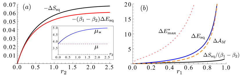
Figure 2: (a) Enhancements in the entropy erased $-\Delta S_{\rm sq}$ in the memory, together with the (scaled) energy flow from the hot to the cold reservoirs, $-{\Delta E}_{\rm sq}$, as a function of the squeezing parameter $r_{2}$, in the case of no squeezing in the cold reservoir, $r_{1}=0$. In the inset figure we show the change in the parameter $\mu_{\ast}$ characterizing the steady state of the memory. (b) Enhancements in the energy extracted from the cold reservoir (blue line), together with the (scaled) entropy produced in the memory $\Delta S_{\rm sq}$ (black line), the coherences flow to the memory $\Delta\mathcal{A}_{M}$ (orange-dashed line), and the maximum extractable energy from the second-law-like inequality in Eq. (IV), $\Delta E_{\rm max}^{\ast}$ (pink-dotted line) in Eq. (54) as a function of the squeezing parameter $r_{1}$, when both reservoirs are squeezed ($r_{2}=0.5$). All quantities are plotted in units of $\hbar\omega$. In both plots we used $\beta_{1}=5/\hbar\omega$, and $\beta_{2}=1.2/\hbar\omega$.

In Figure 2(a) we show the “breaking” of the Landauer’s bound in Eq. (32) when the device acts as an information eraser, $\Delta S_{\mathrm{sq}}<0$. Here we just consider squeezing in the hot reservoir, $r_{2}>0$, while the cold one remains in a thermal state, $r_{1}=0$. In this case we have that the global squeezing amplitude is $r=0$, meaning that the steady state in Eq. (39) is no longer squeezed, but just the Gibbs state $\pi_{\ast}=\exp(\mu_{\ast}N_{M})/Z_{\ast}$. Nevertheless, notice that this corresponds to a lower entropic state than $\pi$ in Eq. (4) since $\mu_{\ast}\geq\mu$ (see inset). As a consequence, we have that introducing squeezing only in the cold thermal reservoir we can erase a greater amount of entropy in the memory. This enhanced erasure indeed overcomes the bound (32), at the cost of inducing a greater amount of energy transferred from the hot to the cold reservoir, represented by the quantity $(\beta_{1}-\beta_{2})\Delta E_{\mathrm{sq}}<0$.

On the other hand, in Fig. 2(b), we show the performance of the device when acting as a Maxwell’s refrigerator. Here we analyze the regime in which both reservoirs contain squeezing, $r_{1},r_{2}>0$. In this case the final state of the memory is squeezed, $r>0$, enabling extra energy extraction from the cold reservoir, $\Delta E_{\mathrm{sq}}$. The asymmetry induced in the memory state, as quantified by $\Delta\mathcal{A}_{M}$, together with the modification of the parameter $\mu_{\ast}$, are responsible of allowing refrigeration on top of the entropy produced in the memory, that is $\Delta S_{\mathrm{sq}}/(\beta_{1}-\beta_{2})$, overcoming again the bound in Eq. (33) for the thermal reservoirs case. Nevertheless, following Eq. (IV) the energy that can be extracted in such process never surpass the bound $\Delta E_{\mathrm{sq}}\leq\Delta E_{\mathrm{max}}^{\ast}$, with

$$\Delta E_{\mathrm{max}}^{\ast}\equiv\frac{\hbar\omega}{\mu_{\ast}}\mathrm{sech}(2r)\Delta S_{\mathrm{sq}}+\tanh(2r)\Delta\mathcal{A}_{M}.$$ (54)

V Conclusions

In this paper, we applied recent results on quantum fluctuation theorems New ; MHP to analyze the thermodynamic impact of squeezing in a Maxwell’s demon setup, where a pure informational component exist. We first explored the simpler case in which a memory system controls the heat flow between thermal reservoirs at different temperatures. We studied the total entropy production in the model both at the level of fluctuations and averages, using a quantum jump approach. We checked the existence of a general fluctuation theorem for the total entropy production in the setup, as well as the conditions for its split into adiabatic and non-adiabatic contributions. This analysis allowed the characterization of the device performance in its principal regimes of operation in Eqs. (32) and (33).

As a second step, we replaced the regular thermal reservoirs by squeezed thermal reservoirs. In this case the entropy changes in the environment are produced by the exchange of both energy and coherence between the nonequilibrium reservoirs. This exchange mechanism is also responsible for inducing squeezing in the memory system at the steady state. The fluctuation theorem for the total entropy production holds as well in this case, but the fundamental processes associated to its increase are no longer simple jumps associated to the exchange of energy quanta between reservoirs. The total entropy production rate is therefore also modified, now including a term proportional to the asymmetry induced by the memory quadratures [Eq. (IV)].

The enhancements in the performance of the device due to the squeezing in the reservoirs can be quantified in this model for situations of specific interest [Eqs. (51)-(52)]. As an example we explored the two different situations represented in Fig. 2. These include Landauer’s erasure at a lower energetic cost when just one of the two thermal reservoirs are squeezed. The second example shows how improvements in the cooling rate of the Maxwell’s refrigerator can be achieved when squeezing is present in both reservoirs. The results presented here pave the way for improved models of quantum devices acting as Maxwell’s demon while profiting from quantum thermodynamical resources like squeezing.

Author contributions

G. M. planned the research, performed the calculations, analyzed the results and wrote the manuscript.

References

- (1) M.B. Plenio and M. Vitelli, Contemp. Phys. 42, (2001) 25-60.
- (2) K. Maruyama, F. Nori, and V. Vedral, Rev. Mod. Phys. 81, (2009) 1.
- (3) J. M. R. Parrondo, J. M. Horowitz, and T. Sagawa, Nat. Phys. 11, (2015) 131-139.
- (4) H. S. Leff and A. F. Rex (Eds.) Maxwell’s Demon 2. Entropy, Classical and Quantum Information, Computing (Taylor and Francis, USA 2002).
- (5) C. H. Bennett, Int. J. Theor. Phys. 21, (1982) 905–940.
- (6) R. Landauer, IBM Journal of Research and Development 5, (1961) 183–191.
- (7) A. Berut, A. Arakelyan, A. Petrosyan, S. Ciliberto, R. Dillenschneider, and E. Lutz, Nature 483, (2012) 187-189.
- (8) J. P. S. Peterson, R. S. Sarthour, A. M. Souza, I. S. Oliveira, J. Goold, K. Modi, D. O. Soares-Pinto, and L. C. Céleri, Proc. Roy. Soc. Lon. A 472, (2016) 20150813.
- (9) D. Mandal and C. Jarzynski, Proc. Natl. Acad. Sci. U.S.A 109, (2012) 11641.
- (10) D. Mandal, H. T. Quan, and C. Jarzynski, Phys. Rev. Lett. 111, (2013) 030602.
- (11) P. Strasberg, G. Schaller, T. Brandes, and M. Esposito, Phys. Rev. Lett. 110, (2013) 040601.
- (12) A. Chapman, and A. Miyake, Phys. Rev. E 92, (2015) 062125.
- (13) C. Elouard, D. Herrera-Martí, B. Huard, and A. Auffèves, Phys. Rev. Lett. 118, (2017) 260603.
- (14) S. Toyabe, T. Sagawa, M. Ueda, E. Muneyuki, and M. Sano, Nat. Phys. 6, (2010) 988–992.
- (15) J. V. Koski, V. F. Maisi, J. P. Pekola, and D. V. Averin, Proc. Natl. Acad. Sci. 111, (2014) 13786–13789.
- (16) E. Roldan, I. A. Martinez, J. M. R. Parrondo, and D. Petrov, Nat. Phys. 10, (2014) 457–461.
- (17) J. V. Koski, A. Kutvonen, I. M. Khaymovich, T. Ala-Nissila, and J. P. Pekola, Phys. Rev. Lett. 115, (2015) 260602.
- (18) M. D. Vidrighin, O. Dahlsten, M. Barbieri, M. S. Kim, V. Vedral, and I. A. Walmsley, Phys. Rev. Lett. 116, (2016) 050401.
- (19) P. A. Camati, J. P. S. Peterson, T. B. Batalhão, K. Micadei, A. M. Souza, R. S. Sarthour, I. S. Oliveira, and R. M. Serra, Phys. Rev. Lett. 117, (2016) 240502.
- (20) N. Cottet, S. Jezouin, L. Bretheau, P. Campagne-Ibarcq, Q. Ficheux, J. Anders, A. Auffèves, R. Azouit, Pierre Rouchon, and B. Huard, Proc. Natl. Acad. Sci. 114, (2017) 7561–7564.
- (21) J. Goold, M. Huber, A. Riera, L. del Rio, and P. Skrzypczyk, J. Phys. A: Math. Theor. 49, (2016) 143001.
- (22) S. Vinjanampathy and J. Anders, Contemp. Phys. 57, (2016) 1–35.
- (23) M. Esposito, K. Lindenberg, and C. Van den Broeck, New J. Phys. 12, (2010) 013013.
- (24) J. P. Pekola, P. Solinas, A. Shnirman, and D. V. Averin, New J. Phys. 15, (2013) 115006.
- (25) D. Reeb and M. M. Wolf, New J. Phys. 16, (2014) 103011.
- (26) S. Suomela, A. Kutvonen, and T. Ala-Nissila, Phys. Rev. E 93, (2016) 062106.
- (27) J. A. Vaccaro and S. M. Barnett, Proc. Roy. Soc. Lon. A 467, (2011) 1770–1778.
- (28) O. Abah, and E. Lutz, Europhys. Lett. 106, (2014) 20001.
- (29) R. Alicki and D. Gelbwaser-Klimovsky, New J. Phys. 17, (2015) 115012.
- (30) P. Strasberg, G. Schaller, T. Brandes, and M. Esposito, Phys. Rev. X 7, (2017) 021003.
- (31) M. O. Scully, M. S. Zubairy, G. S. Agarwal, and H. Walther, Science 299, (2003) 862.
- (32) E. Lutz and R. Dillenschneider, Europhys. Lett. 88, (2009) 50003.
- (33) H. Li, J. Zou, W.-L. Yu, B.-M. Xu, J.-G. Li, and B. Shao, Phys. Rev. E 89, (2014) 052132.
- (34) J. Roßnagel, O. Abah, F. Schmidt-Kaler, K. Singer and E. Lutz, Phys. Rev. Lett. 112, (2014) 030602.
- (35) L. A. Correa, J. P. Palao, D. Alonso, and G. Adesso, Sci. Rep. 4, (2014) 3949.
- (36) A. Ü. C. Hardal and Ö. E. Müstecaploglu, Sci. Rep. 5, (2015) 12953.
- (37) G. Manzano, F. Galve, R. Zambrini, and J. M. R. Parrondo, Phys. Rev. E 93, (2016) 052120.
- (38) W. Niedenzu, D. Gelbwaser-Klimovsky, A. G. Kofman, and G. Kurizki, New J. Phys (2016)
- (39) B. K. Agarwalla, J.-H. Jiang, and D. Segal, Phys. Rev. B 96, (2017) 104304.
- (40) M. Campisi, P. Hänggi, and P. Talkner, Rev. Mod. Phys. 83, (2011) 771.
- (41) M. Esposito, U. Harbola and S. Mukamel, Rev. Mod. Phys. 81, (2009) 1665.
- (42) G. Manzano, J. M. Horowitz, and J. M. R. Parrondo, in press (2017). Preprint at arXiv:1710.00054.
- (43) E. S. Polzik, Nature 453, (2008) 45-46.
- (44) P. D. Drummond and Z. Ficek (Eds.), Quantum Squeezing (Springer-Verlag, Berlin 2004).
- (45) H. Fearn and M. J. Collet, J. Mod. Opt. 35, (1988) 553.
- (46) M. S. Kim, F. A. M. de Oliveira, and P. L. Knight, Phys. Rev. A 40, (1989) 2494.
- (47) B. Yurke, P. G. Kaminsky, R. E. Miller, E. A. Whittaker, A. D. Smith, A. H. Silver, and R. W. Simon, Phys. Rev. Lett. 60, (1988) 764.
- (48) E. E. Wollman, C. U. Lei, A. J. Weinstein, J. Suh, A. Kronwald, F. Marquardt, A. A. Clerk, K. C. Schwab, Science 349, (2015) 952.
- (49) J.-M. Pirkkalainen, E. Damskägg, M. Brandt, F. Massel, and M. A. Sillanpää, Phys. Rev. Lett. 115, (2015) 243601.
- (50) M. Rashid, T. Tufarelli, J. Bateman, J. Vovrosh, D. Hempston, M. S. Kim, and H. Ulbricht, Phys. Rev. Lett. 117, (2016) 273601.
- (51) J. Roßnagel, S. T. Dawkings, K. N. Tolazzi, O. Abah, E. Lutz, F. Schmidt-Kaler, K. Singer, Science 352, (2016) 325-329.
- (52) J. Klaers, S. Faelt, A. Imamoglu, and E. Togan, Phys. Rev. X 7, (2017) 031044.
- (53) M. Büttiker, Z. Phys. B 68, (1987) 161-167.
- (54) R. Landauer, J. Stat. Phys. 53, (1988) 233-248.
- (55) H.-P. Breuer and F. Petruccione, The theory of open quantum systems (Oxford University Press, UK 2002).
- (56) G. Lindblad, Commun. Math. Phys. 48, (1976) 119–130.
- (57) J. M. Horowitz, Phys. Rev. A 85, (2012) 031110.
- (58) J. M. Horowitz, and J. M. R. Parrondo, New J. Phys. 15, (2013) 085028.
- (59) F. W. J. Hekking, and J. P. Pekola, Phys. Rev. Lett. 111, (2013) 093602.
- (60) F. Liu, Phys. Rev. E 89, (2014) 042122.
- (61) F. Liu, Phys. Rev. E 90, (2014) 032121.
- (62) S. Suomela, J. Salmilehto, I. G. Savenko, T. Ala-Nissila, and M. Möttönen, Phys. Rev. E 91, (2015) 022126.
- (63) M. Campisi, J. P. Pekola, and R. Fazio, New. J. Phys. 17, (2015) 035012.
- (64) J. P. Pekola, Y. Masuyama, Y. Nakamura, J. Bergli, and Y. M. Galperin, Phys. Rev. E 91, (2015) 062109; Erratum Phys. Rev. E 92, (2015) 039901.
- (65) G. Manzano, J. M. Horowitz, and J. M. R. Parrondo, Phys. Rev. E 92, (2015) 03212.
- (66) C. Elouard, D. A. Herrera-Martí, M. Clusel, and A. Auffèves, npj Quantum Information 3, (2017) 9.
- (67) H. M. Wiseman, and G. J. Milburn, Quantum measurement and Control (Cambridge University Press, UK 2010).
- (68) U. Seifert, Phys. Rev. Lett. 95, (2005) 040602.
- (69) T. Sagawa, Second law-like inequalitites with quantum relative entropy: An introduction in Lectures on quantum computing, thermodynamics and statistical physics. Kinki University Series on Quantum Computing. (World Scientific, USA 2013).
- (70) M. Esposito and C. Van den Broeck, Phys. Rev. Lett. 104, (2010) 090601
- (71) M. Esposito and C. Van den Broeck, Phys. Rev. E 82, (2010) 011143; 011144.
- (72) U. Seifert, Rep. Prog. Phys. 75, (2012) 126001.
- (73) G. E. Crooks, Phys. Rev. A 77, (2008) 034101.
- (74) P. Hänggi and H. Thomas, Phys. Rep. 88, (1982) 207-319.
- (75) T. Hatano, and S.-i. Sasa, Phys. Rev. Lett. 86, (2001) 3463.
- (76) J. Prost, J.-F. Joanny, and J. M. R. Parrondo, Phys. Rev. Lett. 103, (2009) 090601.