Luminosities and mass-loss rates of Local Group AGB stars and Red Supergiants

Abstract

Context. Mass loss is one of the fundamental properties of asymptotic giant branch (AGB) stars, and through the enrichment of the interstellar medium, AGB stars are key players in the life cycle of dust and gas in the universe. However, a quantitative understanding of the mass-loss process is still largely lacking.

Aims. We aim to investigate mass loss and luminosity in a large sample of evolved stars in several Local Group galaxies with a variety of metalliticies and star-formation histories: the Small and Large Magellanic Cloud, and the Fornax, Carina, and Sculptor dwarf spheroidal galaxies (dSphs).

Methods. Dust radiative transfer models are presented for 225 carbon stars and 171 oxygen-rich evolved stars in several Local Group galaxies for which spectra from the Infrared Spectrograph on Spitzer are available. The spectra are complemented with available optical and infrared photometry to construct spectral energy distributions. A minimization procedure was used to determine luminosity and mass-loss rate (MLR). Pulsation periods were derived for a large fraction of the sample based on a re-analysis of existing data.

Results. New deep $K$-band photometry from the VMC survey and multi-epoch data from IRAC (at 4.5 $\mu$m) and AllWISE and NEOWISE have allowed us to derive pulsation periods longer than 1000 days for some of the most heavily obscured and reddened objects. We derive (dust) MLRs and luminosities for the entire sample. The estimated MLRs can differ significantly from estimates for the same objects in the literature due to differences in adopted optical constants (up to factors of several) and details in the radiative transfer modelling. Updated parameters for the super-AGB candidate MSX SMC 055 (IRAS 00483$-$7347) are presented. Its current mass is estimated to be 8.5 $\pm$ 1.6 $M_{\odot}$, suggesting an initial mass well above 8 $M_{\odot}$ in agreement with estimates based on its large Rubidium abundance. Using synthetic photometry, we present and discuss colour-colour and colour-magnitude diagrams which can be expected from the James Webb Space Telescope.

1 Introduction

Almost all stars with initial masses in the range $\sim$ 0.9–8 $M_{\odot}$ will pass through the asymptotic giant branch (AGB) phase, which is the final stage of active nuclear burning before they become post-AGB objects, planetary nebulae and finally white dwarfs. Stars above this mass range will pass through the red supergiant (RSG) phase before they may end as supernovae. In both cases, mass loss dominates the final evolutionary stages of the star.

The Infrared Astronomical Satellite (IRAS) and the Infrared Space Observatory (ISO) have greatly improved our understanding of these final evolutionary stages for stars in the Galaxy, but uncertainties in distances prevent accurate luminosities and mass-loss rates (MLRs). Sources at known distances, as in the Large and Small Magellanic Clouds (LMC and SMC), or nearby dwarf spheroidal galaxies (dSphs), reduce this problem and also enable the study of the effect of metallicity on the MLR. Surveys of the Magellanic Clouds (MCs) with the Spitzer Space Telescope (Werner et al. 2004) have added to this legacy with data from IRAC (Fazio et al. 2004) and MIPS (Rieke et al. 2004): the Spitzer Survey of the SMC (S³MC; Bolatto et al. 2007) and the full-galaxy catalogues from Surveying the Agents of Galactic Evolution program for the LMC (Meixner et al. 2006) and SMC (Gordon et al. 2011).

Groenewegen et al. (2007) previously modelled the spectral energy distributions (SEDs) and spectra taken with the Infrared Spectrograph (IRS; Houck et al. 2004) on board Spitzer for a sample of 60 carbon (C) stars. Groenewegen et al. (2009, hereafter G09) extended this to 101 C stars and 86 oxygen-rich AGB stars and RSGs (hereafter referred to as M stars for simplicity) in the MCs.

The cryogenic phase of the Spitzer mission is over and the data taken with the IRS spectrograph are publicly available, for example through the CASSIS website (Lebouteiller et al. 2011). In this paper we investigate a sample of AGB stars and RSGs in the MCs that is almost double in size compared to that considered by G09, including 19 C stars in four dSphs: Fornax, Carina, Leo I, and Sculptor (Matsuura et al. 2007, Sloan et al. 2012).

Considerable work is ongoing to model large numbers of AGB stars in the MCs using the available photometry, by fitting the SEDs of individual stars with a radiative transfer model. Gullieuszik et al. (2012) presented results on 374 AGB candidates in a 1.42 square degree area in the LMC observed as part of the VISTA Magellanic Cloud Survey (VMC; Cioni et al. 2011). Riebel et al. (2012) derived MLRs for a sample of $\sim$30 000 AGB stars and RSGs in the LMC, by fitting up to 12 bands of photometry to the precomputed Grid of Red Supergiant and Asymptotic Giant Branch ModelS (GRAMS; Srinivasan et al. 2011 for the C-rich grid; Sargent et al. 2011 for the O-rich grid). Srinivasan et al. (2016) used a similar approach for the SMC. Boyer et al. (2012) took a hybrid approach by first determining the dust MLR using the GRAMS models for 65 stars in five classes of AGB stars and RSGs. They then determined relations between the dust MLR and photometric excess at 8 $\mu$m and used these to estimate the dust MLR for a total of about 25 000 AGB stars and RSGs in the LMC and about 7500 in the SMC.

To only consider stars with IRS spectra naturally limits the number of stars for which mass-loss rates and luminosities may be determined, but the spectra provide some important advantages compared to just a photometric sample. First, molecular absorption bands and dust emission features in the spectra allow confident identifications of C-rich versus O-rich stars (as described succinctly by Kraemer et al. 2002). Spectroscopic classifications are not perfect, primarily because some sources exhibit C-rich and O-rich characteristics simultaneously, but they do help break the degeneracies where the two classes overlap in colour-colour space (for the bluest and reddest sources). Second, the spectra better constrain mineralogical properties of the dust such as grain size and shape, crystallinity, and chemistry. And, because the spectra provide more information on a source than the photometry can, they also better constrain the radiative transfer models fitted to the data. The lessons learned from the smaller spectroscopic sample can then be applied to models of the much larger photometric samples.

Section 2 describes the sample of AGB stars and RSGs with IRS spectra and the spectral data. Section 3 describes the ancillary photometry and the periods derived from those data. Section 4 presents the radiative transfer model and the properties of the dust species considered. Section 5 presents the results and compares them to previous efforts (e.g. G09). In Sect. 6 we discuss the relation between stellar evolution and mass loss.

2 The sample of infrared spectra

2.1 Spectra

Several groups have obtained Spitzer IRS data of evolved stars in the LMC and SMC. Table 1 lists the programs considered here. The last program listed provided data on a sample of 19 C stars in the Carina, Fornax, Leo I, and Sculptor dSphs.

Table 1: Spectroscopic Spitzer programs considered in this paper.

Program	Principal	Reference paper	Notes
ID	investigator
200	J. R. Houck	Sloan et al. (2008)	Evolved stars in the LMC and SMC
1094	F. Kemper		AGB evolution in the LMC (and Galaxy)
3277	M. P. Egan	Sloan et al. (2006), Kraemer et al. (2016)	Infrared-bright sample in the SMC
3426	J. H. Kastner	Buchanan et al. (2006)	Infrared-bright sample in the LMC
3505	P. R. Wood	Zijlstra et al. (2006), Lagadec et al. (2007)	AGB stars in the LMC and SMC
3591	F. Kemper	Leisenring et al. (2008)	Evolved O-rich stars in the LMC
30155	J. R. Houck		Sources with crystalline silicates in the SMC
30788	R. Sahai	Sloan et al. (2014)	Embedded carbon stars and post-AGB objects in the LMC
40159	A. Tielens	Kemper et al. (2010), Woods et al. (2011)	Filling colour-colour and colour-mag. space in the LMC
40650	L. W. Looney	Gruendl et al. (2008)	YSOs (and some deeply embedded carbon stars) in the LMC
50167	G. Clayton		RSGs in the LMC and SMC
50240	G. C. Sloan		Filling colour-colour and colour-mag. space in the SMC
50338	M. Matsuura	Matsuura et al. (2014)	Carbon-rich post-AGB candidates in the LMC
20357	A. Zijlstra	Sloan et al. (2012)	Carbon stars in other Local Group dwarf galaxies

Most of the spectra considered here were obtained with the low-resolution modules of the IRS: Short-Low (SL), which covers the 5.1–14.2 $\mu$m range, and Long-Low (LL), which covers 14.0–37.0 $\mu$m. Both modules have a resolution ($\lambda$/$\Delta$$\lambda$) of $\sim$60–100. For some of the fainter sources, spectra were obtained using only SL. Program 40650 (Gruendl et al. 2008) observed several deeply embedded carbon-rich sources with SL and the two modules with higher spectral resolution, Short-High (SH) and Long-High (LH). They referred to these sources as extremely red objects (EROs), and we have done the same.

All observations utilized the standard IRS nodding mode, which produces spectra of the source in two positions in each slit. Each module has two apertures, which produce spectra in two orders, along with a short ‘bonus’ order, which produces a short piece of the first-order spectrum when the source is in the second-order aperture. Thus, to generate a full low-resolution IRS spectrum, eight separate pointings of the telescope are required, and these produce 12 spectral segments which must be combined.

The detailed nature of the observations varied substantially among the samples considered here. Some observers were careful to match the integration times and number of integration cycles in each aperture of a given module; others prioritized reduced observing time over flexibility in background subtraction. Whenever possible, we differenced images by aperture in SL, using the image with the source in one aperture as the background for the image when the source is in the other aperture. For LL, we generally used the image with the source in one nod as the background for an image with the source in the other nod in the same aperture. However, when forced to deviate from this default due to background gradients, other sources in the image, or the design of the observation, we shifted to whatever background had the least structure. Difference images still contain pixels which cannot be calibrated (rogue pixels), which we replaced using the imclean algorithm (see Sloan & Ludovici (2012) for more details).

Spectra were extracted from images using two methods: tapered-column and optimal extraction. The former sums the spectra within a range of fractional pixels close to the spectral trace. The algorithms available with the SMART and CUPID packages are functionally equivalent; we used CUPID. Optimal extraction fits a measured point-spread function (PSF) to the image at each wavelength to minimize the noise. We used the algorithm available in SMART (see Lebouteiller et al. 2010 for details) but ran it offline.

For tapered-column extraction, spectra were extracted from individual images and then co-added. For optimal extraction, we coadded the images first to improve our ability to properly locate faint sources, then extracted.

The tapered-column extractions are preferred in only a few cases. If the source is extended, optimal extraction produces artefacts due to the impossibility of fitting a PSF. For bright sources, the gain in signal-to-noise ratio (SNR) with the optimal extraction is negligible, and for the highest SNR cases, artefacts due to limits in our understanding of the PSF can be seen. We used optimal extraction in most cases; it can improve the SNR by a factor of nearly two. Only when the spectra produced different structure did we rely on the tapered-column extraction. Most of the spectra considered here are publicly available from the CASSIS website, which provides both tapered-column and optimal extractions and guidance as to which is preferred in individual cases.

Spectra observed with SH and LH were extracted using full-slit extraction, which is also available in SMART. Only the EROs from Program 40650 (Gruendl et al. 2008) are affected.

Another difference between observations was the requested accuracy of the peak-up algorithm used to centre the source in the spectroscopic slit. Some of the spectra did not utilize the highest accuracy, and as a result these were more likely to suffer from partial truncation of the source by the slit edges. Given the narrow size of the SL slit (3.6″) compared to the typical pointing accuracy of $\sim$0.4″, any of the SL data could be affected. Sloan & Ludovici (2012) found that for most observations, multiplying a spectral segment by a scalar would solve this pointing-induced throughput problem to within $\sim$2%.

Throughput problems generally result in small discontinuities between spectral segments. We assumed that all corrections should be up, to the best-centred spectral segment.

We calibrated the spectra using HR 6348 (K0 III) as a standard star, supplemented with HD 173511 (K5 III) for LL data taken after the change in detector settings for that instrument (starting with IRS Campaign 45). Sloan et al. (2015) describe how the truth spectra for these sources were constructed, tested, and cross-calibrated with other systems.

2.2 Considering the sample

Not all programs considered here observed AGB stars and RSGs exclusively. As with G09, targets were selected from these programs by examining the IRS spectra, collecting additional photometry (see below), consulting SIMBAD and the papers describing these programs, and considering the results of the radiative transfer modelling (see Sect. 4).

Our classification leads to a sample with 225 C stars and 171 M stars, with the M stars including ten objects in the foreground of the LMC and one in front of the SMC. Our C stars include R CrB stars and post-AGB objects which other groups place in separate categories. For example, we count 160 stars in the LMC and 46 in the SMC, while Sloan et al. (2016) count 144 and 40, respectively. The classifications from the SAGE Team include 145 C stars in the LMC and 39 in the SMC (Jones et al. 2017b; Ruffle et al. 2015). We have classified one unusual object, 2MASS J00445256$-$7318258 (j004452) as a C star, due to the deep C₂H₂ absorption band centred at 13.7 $\mu$m. Ruffle et al. (2015) classify it as O-rich due to the presence of strong crystalline emission features at 23, 28, and 33 $\mu$m. Kraemer et al. (2017; They refer to the object as MSX SMC 049.) confirmed its optical C-rich spectrum, noted its dual C/O chemistry in the mid-infrared, and suggested that it may be a post-AGB object.

3 Ancillary data

Tables 20 and 21 in the Appendix list basic information for the C and M stars respectively, including name, position, an abbreviated identifier used in subsequent tables and figures, the pulsation period, pulsation (semi-)amplitude and filter (see details in Section 3.2 below), and remarks. These tables and some of the figures use the following classifiers for the oxygen-rich stars: FG=Foreground; SG=Supergiant; MA=M-type AGB-star.

3.1 Photometry

For all stars additional broadband photometry ranging from the optical to the mid-IR was collected from the literature, primarily using VizieR and the NASA/IPAC Infrared Science Archive, using the coordinates given in Tables 20 and  21.

In the optical we collected $UBVI$ data from Zaritsky et al. (2002, 2004) for the LMC and SMC, $UBVR$ data from Massey (2002) for the MCs, $BVRI$ data from Oestreicher et al. (1997) for RSGs in the LMC, OGLE-iii $VI$ mean magnitudes from Udalski et al. (2008a,b), EROS $BR$ mean magnitudes from Kim et al. (2014) and Spano et al. (2011), MACHO $BR$ mean magnitudes from Fraser et al. (2008), and $VRI$ data from Wood, Bessell & Fox (1983, hereafter WBF).

Near-infrared photometry comes from DENIS $IJK$ data from Cioni et al. (2000) and their third data release (The DENIS consortium 2005), the all-sky $JHK$ release of 2MASS (Skrutskie et al. 2006), the extended mission long-exposure release (2MASS-6X, Cutri et al. 2006), $JHK$ data from the IRSF survey (Kato et al. 2007), $JHK$ data from the LMC near-infrared synoptic survey (Macri et al. 2015), SAAO $JHKL$ data from Whitelock et al. (1989, 2003), and CASPIR $JHKL$ data specifically taken for the IRS observations (Sloan et al. 2006, 2008, Groenewegen et al. 2007), and from Wood et al. (1992), and Wood (1998). VMC data (Cioni et al. 2011) were used for selected very red sources, mostly to try to determine their pulsation periods (Sect. 3.2).

Mid-infrared data include IRAS data from the Point Source Catalogue and the Faint Source Catalogue (Moshir et al. 1989; Loup et al. 1997; only data of the highest quality flag were considered), photometry at 3.6, 4.5, 5.8, 8.0 and 24 $\mu$m from the SAGE survey of the LMC (Meixner et al. 2006; two epochs), the S³MC survey of the SMC, (Bolatto et al. 2007), and the SAGE-SMC catalogue (Gordon et al. 2011; also two epochs). For selected very red sources we also used Spitzer photometric data from Gruendl et al. (2008) and Whitney et al. (2008). We also used data from the Wide-field Infrared Survey Explorer (WISE; Wright et al. 2010), specifically from the AllWISE catalogue (Cutri et al. 2013), as well as data from the Akari Point-Source Catalogueue (up to five filters between 3 and 24 $\mu$m) and Infrared Camera catalogue (IRC; 9 and 11 $\mu$m) (Ishihara et al. 2010, Ita et al. 2010, Kato et al. 2012).

Far-infrared data were obtained from the Akari Far-Infrared Surveyor (FIS, with four filters between 65 and 160 $\mu$m; Yamamura et al. 2010), MIPS 70 $\mu$m data from the SAGE survey, and the Heritage survey, which included photometry from Herschel at 70, 100, 250, 350, and 500 $\mu$m (Meixner et al. 2013). Reliable data beyond 60 $\mu$m were available for only about a dozen C stars and a half dozen O stars, mostly SAGE data at 70 $\mu$m. Additionally, MIPS-SED spectra (van Loon et al. 2010a,b) were used for four sources.

The literature considered is not exhaustive, but it does include all recent survey data available in the near- and mid-IR, where these stars emit most of their energy. When fitting radiative transfer models, all data were considered as individual measurements with their reported errors. No attempt was made to combine or average multiple observations in a given photometric band, or in similar bands from different telescopes. Variability is an important characteristic of AGB stars and can influence the constructed SED and the fitting. Fortunately, in the optical where the amplitude of variability is largest, mean magnitudes are available from the OGLE, MACHO and EROS surveys, with small errors on the mean magnitude.

In most cases, spectra from the IRS and the infrared photometry agreed. In the 48 cases where they did not ($\sim$ 12% of the sample), the spectra were scaled to the available photometry in wavelengths covered by the spectrum. In half of those cases, the correction was less than 25%, and in 14 cases it was larger than a factor of two.

3.2 Pulsation periods

An extensive effort was made to obtain pulsation periods for the sample. The most important data sources are the OGLE, EROS and MACHO photometric surveys. Although periods have been published for LPVs from these surveys, we downloaded the original data and derived periods independently using the publicly available code Period04 (Lenz & Breger 2005). OGLE-III $I$-band data are available through the OGLE Catalogue of Variable Stars. The EROS-2 data for more than 150 000 stars that were used by Kim et al. (2014) are available online, and the data for the few stars that were missing were kindly provided by Dr. Jean-Baptiste Marquette (private communication). The correspondence between EROS-2 identifier and coordinates is provided by a separate database, but is also available through SIMBAD and VizieR. MACHO data are also online. In this case any association listed in SIMBAD and VizieR between our sources and the MACHO counterpart was only taken as guidance, and we independently searched for all MACHO targets within 2.5″ of our targets.

Other sources of optical data were also considered, specifically the Catalina Sky Survey (CSS, Drake et al. 2014), ASAS-3 data (Pojmanski 2002), and data from the Optical Monitor Camera (OMC) onboard INTEGRAL (Mas-Hesse et al. 2011).

Many of the redder sources have traditionally been monitored in the near-infrared (for example Wood 1998, Whitelock et al. 2003), and these data have also been used, either taking directly the quoted periods and amplitudes or in some cases combining the data and rederiving the periods. For red stars with no previous period determination or where the available infrared data were sparse, the VMC database (Cioni et al. 2011) was consulted. In the $K$-band the VMC observations typically have 10–15 data points spread over a relatively short timespan (6–12 months), but when combined with other data, even if from a single epoch, a reliable and unique period could be derived in many cases (Groenewegen et al. in prep.)

To analyse the variability of the more embedded sources, we have used the data from WISE differently than described in the previous section, where the focus was on assembling photometric data to be fitted with radiative transfer models. To investigate variability, we have followed Sloan et al. (2016) and used the AllWISE Multiepoch Photometry Table and the NEOWISE-R Single Exposure (L1b) Source Table (from the NEOWISE reactivation mission; Mainzer et al. 2014) but with some changes to their method. We did not average together data taken within a few days of each other. We considered data up to and including the June 2017 release, which gives two more years of data than were considered before. We also focussed just on the W2 filter at 4.6 $\mu$m, as it is brighter than W1 for the reddest sources.

When data were available, we combined the W2 data with IRAC 4.5 $\mu$m data from the SAGE-VAR catalogue (Riebel et al. 2015), which adds four epochs obtained during the warm Spitzer mission on the Bar of the LMC and the core of the SMC with the original epochs obtained during the SAGE and SAGE-SMC surveys. The effective wavelengths of the W2 and IRAC 4.5 filters are similar, but for the reddest sources for which these data were used, the difference can be of the order of a few tenths of a magnitude. To shift the W2 at 4.6 $\mu$m to 4.5 $\mu$m, we did not use the colour corrections derived by Sloan et al. (2016). Instead, we used the radiative transfer models fitted to the photometry to determine the proper adjustment from the WISE to the IRAC filter.

Tables 20 and 21 in the Appendix list the adopted pulsation period, the amplitude (in the mathematical sense, sometimes referred to as the semi-amplitude, or in other words, half the peak-to-peak amplitude), the filter, and the reference to the data used.

The sample includes about 180 stars with periods listed by OGLE. In 85% (88%) of the cases the period we derive from the OGLE data agrees within 5% (10%) with the first of three possible periods listed by OGLE. In an additional 6% of the cases our adopted pulsation period corresponds to the second period listed by OGLE. There are also a few cases where the period we find is about double that of the first OGLE period. The final periods listed in the tables also include the analysis from EROS and MACHO data when available.

As mentioned above, Sloan et al. (2016) used AllWISE and NEOWISE data to derive previously unknown periods for five C stars (their Fig. 20). For three stars we quote periods here based on $K$-band data from the VMC survey and the literature (Groenewegen et al. in prep), that agree to within 3% with the periods found by Sloan et al. For the other two stars, we independently derived the periods based on the W2 filter (combining it with [4.5] data for one object). Despite the differences in our approaches, the periods agree within 1%.

4 The model

The models are based on the ‘More of DUSTY’ (MoD) code (Groenewegen 2012) which uses a slightly updated and modified version of the DUSTY dust radiative transfer (RT) code (Ivezić et al. 1999) as a subroutine within a minimization algorithm.

4.1 Running the radiative transfer code

The RT code determines the best-fitting dust optical depth, luminosity, temperature at the inner radius, $T_{\rm c}$, and index of the density distribution, $\rho\sim r^{-p}$ by fitting photometric data and spectra for a given model atmosphere and dust composition. (The code can also consider visibility data and 1D intensity profiles, but these data are not available for the sample considered here.) Each of the four free parameters may be fixed or fitted in the RT code, see Section 4.3.

The outer radius in the models is set to a value where the dust temperature reaches about 20 K. This implies values of $(4-22)\cdot 10^{3}$ times the inner radius, which correspond to outer radii of less than $\sim 25\arcsec$ in all cases. However, depending on wavelength, the emission comes from a much smaller region. As a test, the SED was calculated for one of the reddest sources with a large default outer radius of $13\leavevmode\nobreak\ 000\leavevmode\nobreak\ R_{\rm in}$, and then re-run with progressively smaller outer radii. At 70 $\mu$m the flux is reduced by 5% when decreasing the outer radius to $2\leavevmode\nobreak\ 000\leavevmode\nobreak\ R_{\rm in}$, corresponding to about 2″. In comparison the FWHM of the MIPS 70 $\mu$m band is 18″. Emission at shorter wavelengths comes from an even more compact region, for example $\stackrel{{\scriptstyle<}}{{\sim}}$ 1″ at 24 $\mu$m. Generally, the PSFs of the combinations of instrument and filter of the datasets listed in Sect. 3 match the physical size of the emitting region at the distance of the MCs quite well. The exception is the WISE 4 filter at 22 $\mu$m with a PSF of 12″, which is much larger then the size of the emitting region and makes background subtraction more important. In fact, this is the data point that has been excluded most frequently from the SEDs, in 25 of the 370 sources for which it was available.

We masked those portions of the IRS spectra with poor S/N or those affected by background subtraction problems and did not include them in the minimization procedure. In addition, spectral regions dominated by strong molecular features that are not included in the simple model atmospheres are also excluded for the C stars, that is the regions 5.0–6.2 $\mu$m (CO + C₃, e.g. Jørgensen et al. 2000), 6.6–8.5 $\mu$m and 13.5–13.9 $\mu$m (C₂H₂, e.g. Matsuura et al. 2006). No regions were excluded in the fitting of the O-rich stars.

The photospheric models for C stars come from Aringer et al. (2009), while the M stars are modelled by a MARCS stellar photosphere model (Gustafsson et al. 2008). For the C stars, the models assume 1/3 solar metallicity for the LMC and 1/10 for the SMC and other Local Group galaxies. For M stars, the corresponding values are $-0.5$ and $-0.75$ dex. The model atmospheres also depend on $\log g$, mass, and C/O ratio (for the C-stars). The SED fitting is not sensitive to these values, and we adopted fixed values $\log g=0.0$ or $+0.5$, 1 or 2 $M_{\odot}$, and C/O= 1.4.

To determine luminosities from the RT output, distances of 50 kpc to the LMC and 61 kpc to the SMC are adopted, while for the other Local Group galaxies the distances adopted by Sloan et al. (2012) are kept: 84.7 kpc for Sculptor, 104.7 kpc for Carina, 140.6 kpc for Fornax, and 259.4 kpc for Leo I.

The model results have been corrected for a typical $A_{\rm V}$ = 0.15 mag for all Magellanic stars, 0.06 mag for Sculptor, 0.08 mag for Carina and Fornax, and 0.09 mag for Leo I. We adopted the reddening law of Cardelli et al. (1989) for other wavelengths. The exact value has little impact on the results, as it corresponds to $\stackrel{{\scriptstyle<}}{{\sim}}$0.02 mag of extinction in the near-IR.

4.2 Dust grain properties

The dust around the C stars is assumed to be a combination of amorphous carbon (AMC), silicon carbide (SiC), and magnesium sulphide (MgS). The optical constants are taken from Zubko et al. (1996, the ACAR species, denoted ‘zubko’ in Table 22) for AMC, Pitman et al. (2008, denoted ‘Pitm’ in Table 22) for SiC, and Hofmeister et al. (2003, denoted ‘Hofm’ in Table 22) for MgS.

Models were run mostly for a single grain size 0.15 $\mu$m, although some models were also explored with $a$= 0.10 and 0.30 $\mu$m. The current modelling does not allow us to determine the grain size (or even grain size distribution). Nanni et al. (2016) recently found that the near- and mid-IR colours of SMC C-stars can be described better with grains of size $\stackrel{{\scriptstyle<}}{{\sim}}$0.12 $\mu$m than with grains $\stackrel{{\scriptstyle>}}{{\sim}}$0.2 $\mu$m.

The models by G09 did not consider MgS, and the 22–39 $\mu$m wavelength range was specifically excluded in their fitting. Also, the absorption and scattering coefficients were calculated in the small-particle limit for spherical grains. Here, MgS is included in the fitting, but spherical grains are known not to match the observed profile of MgS (Hony et al. 2002). The absoption and scattering coefficients for MgS have been calculated using a distribution of form factors (Mutschke et al. 2009) close to the classical CDE (continous distribution of ellipsoids; see Min et al. 2006). This distribution fits the observed shape of the 30 $\mu$m feature reasonably well.

The identification of MgS as the carrier of the 30 $\mu$m feature by Goebel & Moseley (1985) has come under some scrutiny in the past few years. The primary issue is that the strength of the 30 $\mu$m feature in some post-AGB objects would violate abundance limits if the grains were solid MgS (Zhang et al. 2009). However, if MgS forms a layer on a pre-existing core, it will produce the observed feature without requiring too much Mg or S. Sloan et al. (2014) reviewed the spectroscopic evidence supporting the case for layered grains, addressed other concerns about MgS as the carrier of the 30 $\mu$m feature, and concluded that it remains the best candidate.

The absorption and scattering coefficients for SiC and AMC are calculated using a distribution of hollow spheres (DHS, Min et al. 2003). In DHS, the optical properties are averaged over a uniform distribution in volume fraction between zero and $f_{\rm max}$ of a vacuum core, where the material volume is kept constant, in order to simulate the fluffiness of real grains. G09 found that $f_{\rm max}=0.7$ fitted the data well, and we use that value here.

AMC, SiC and MgS are then mixed in proportions in order to fit the data, that is the strength of the SiC and MgS feature. This method assumes that the mixture is uniform throughout the envelope and that the grains are in thermal contact.

For M stars the dust chemistry is richer than that for C stars. We considered several species, but found that we could model the observed data with four dust components: amorphous silicates (olivine or MgFeSiO₄; Dorschner et al. 1995; denoted ‘Oliv’ in Table 23), amorphous alumina (Begemann et al. 1997; denoted ‘AlOx’), metallic iron (Pollack et al. 1994; denoted ‘Fe’), and crystalline forsterite (Mg_1.9Fe_0.1SiO₄; Fabian et al. 2001, denoted ‘Forst’).

The absorption and scattering coefficients are calculated using DHS with $f_{\rm max}=0.7$, and for grain sizes 0.1, 0.2 and 0.5 $\mu$m, compared to a more traditional value of $\sim$0.1 $\mu$m. For some Galactic targets, large grains have proven necessary when near-IR visibility data are available, because they provide an additional scattering component. Examples include IRC +10 216 and OH 26.5, which were fitted with MoD code by Groenewegen et al. (2012) and Groenewegen (2012), respectively. Recently, Norris et al. (2012), Scicluna et al. (2015), and Ohnaka et al. (2016) found evidence for grains in the range 0.3–0.5 $\mu$m, and 0.1–1 $\mu$m grains are advocated to drive the outlow around oxygen-rich stars (Höfner 2008, Bladh & Höfner 2012).

4.3 Finding the best model

The MoD code determines the best-fitting luminosity, dust optical depth, temperature at the inner radius, and index of the density distribution. Groenewegen (2012) describes how to identify the best-fitting model by minimizing a $\chi^{2}$ parameter.

The luminosity is fitted in all cases. Whether the other three parameters have been fitted or fixed is indicated in Tables 22 and 23. In about 8% of the objects, the data show no evidence of a dust excess, and the dust optical depth is fixed to a small value. In about one-third of the C-stars and half of the O-stars, the dust optical depth is the only additional free parameter. When not fitted, $T_{\rm c}$ is fixed to the typical condensation temperature (1200 K for C-stars and 1000 K for O-stars in most cases) and $p$ is fixed to two, that is the density law for a constant outflow velocity and MLR.

Increasing the number of free parameters will always decrease the reduced $\chi^{2}$ of the model. To avoid overfitting and penalizing the addition of free parameters, MoD also calculates the Bayesian information criterion (BIC; Schwarz 1978; see also Groenewegen 2012). The best-fitting model is the one with the lowest BIC value.

Some of the parameters that are determined are external to MoD, as they are available on a discrete grid only. For example, the model atmospheres (both MARCS and Aringer et al. 2009) are available on a grid with 100 K spacing. In addition, the grain absorption and scattering properties are pre-calculated for a discrete number of grain sizes and dust compositions. For C stars, we considered AMC, SiC and MgS in ratios 100 : $x$ : $y$, where $x$ and $y$ are integer multiples of five. We treated O-rich stars with a similar grid for silicates, alumina, metallic iron and forsterite.

MoD is then run over the grid of effective temperatures (for a typical dust composition) to find the best-fitting model atmosphere. Then the model atmosphere is fixed to that effective temperature, and the model is run over the grid of grain sizes and dust compositions to find the best dust model. The input and output of the models (parameters, reduced $\chi^{2}$, BIC) are stored, so that the lowest BIC (the best-fitting model) may be found, and errors estimated for the parameters.

5 Results

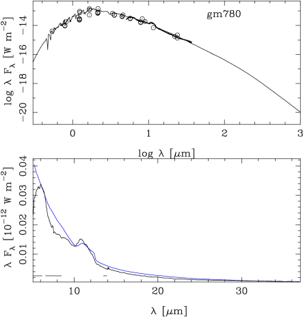
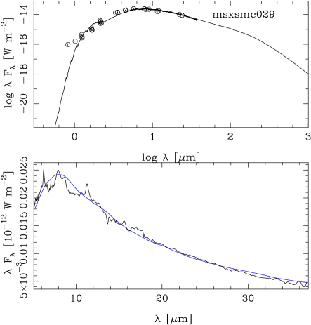
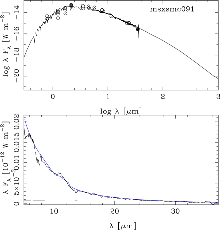
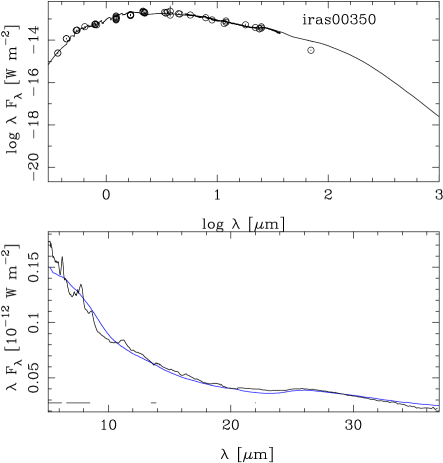
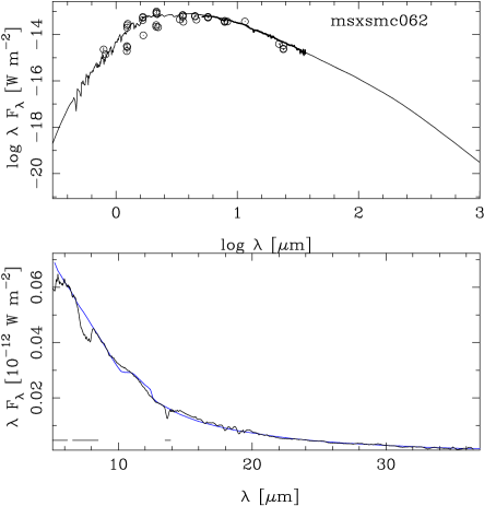
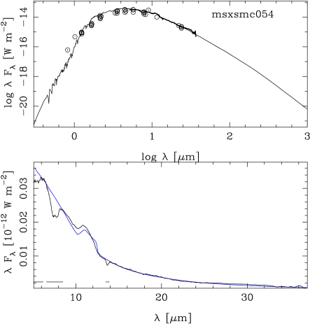
Figure 11: Fits to the SEDs and IRS spectra of C stars. In the upper panel the model (the continuous line) is shown with the IRS spectrum and the photometric points on a logarithmic scale. The lower panel shows the IRS spectrum and model in more detail on a linear scale. The model has been fit to the data by scaling to a quasi-continuum point based on the average flux in the 6.4–6.5 $\mu$m region. Horizontal lines near the bottom indicate wavelength regions excluded from the fit.

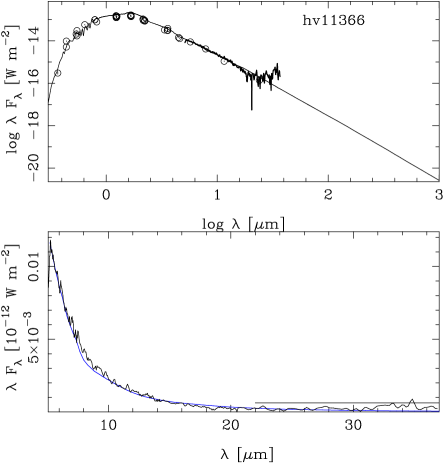
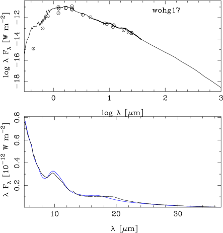
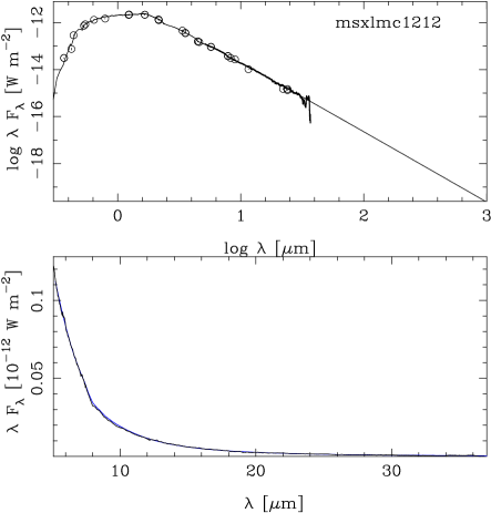
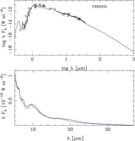
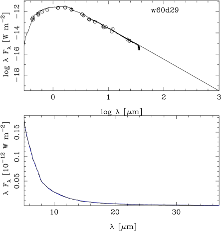
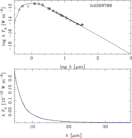
Figure 2: As Figure 11 for the O stars.

Tables 22 and 23 in the Appendix list the parameters of the models which best fit the observed data for the C stars and M stars, respectively. Figures 11 and 2 in the Appendix show the best-fitting model to the SED and IRS spectra for these two groups. The tables include the luminosity and MLR, calculated assuming an expansion velocity v_exp of 10 km s^-1 and a gas-to-dust ratio of 200. Observations of CO line widths suggest that the outflow velocity may depend on luminosity and metallicity (e.g. van Loon et al. 2000, Lagadec et al. 2010, Groenewegen et al. 2016; Goldman et al. 2017). The gas-to-dust ratio in the circumstellar outflows is expected to scale with the initial metallicity for O rich sources, but this is not clear for C rich sources, which fuse carbon in their interiors. In both cases, though, the nature of that dependence is uncertain, and we hold both velocity and gas-to-dust ratio constant to aid comparison. The MLRs are proportional to both quantities and can be scaled as desired.

The fitting routine also provides uncertainties for the MLR, dust temperature at the inner radius, and luminosity. These are typically small, of order 1%, and are not reported. The realistic 1$\sigma$ errors are larger, and can be estimated from a comparison of model runs with different parameters and different realizations of the photometric data. They are typically 10% in luminosity, 25% in MLR and 50 K in $T_{\rm c}$, and have been estimated from the spread in the parameters in all models that have a $\chi^{2}$ less than twice the value of the best-fitting model. The difference between the small fitting error and the realistic error is likely due to the difficult treatment of source variability in the fitting. Currently, multiple measurements at a given wavelength have been assigned their respective photometric errors. However, the source variability, especially in Miras and long-period variables is usually much larger than the photometric uncertainty. The fitting will lead to a larger best-fit $\chi^{2}$ than if the same source were only fitted with, say, a single $K$-band photometric point.

5.1 Colour relations

Some of the analysis presented by G09 can be improved here thanks to the larger sample size. Figure 1 shows a synthetic colour-colour diagram (CCD) generated from the best-fitting models. Plotting [5.8]$-$[8.0] vs. [8.0]$-$[24] is effective at distinguishing M from C stars (Kastner et al. 2008, G09). The larger sample only reinforces this conclusion. Following this result, we also constructed CCDs with similar colours generated by using WISE and Akari data. For WISE data, W2$-$W3 vs. W3$-$W4 has the most discriminatory power, and for Akari, it is N4$-$S7 vs. S7$-$L24. Both CCDs show behaviour similar to the Spitzer-based CCD, but they do not separate the M and C stars quite as well.

Figure 1: Colour-colour diagrams for the SMC (left-hand panels) and LMC (right-hand panels). Top panels: the combination of IRAC and MIPS colours from Spitzer. Middle panels: WISE colours. Bottom panels: Akari colours. Symbols are explained in the legend. The lines indicate the border between C- and O-rich stars (see text).

Figure 2: Colour-colour diagrams for the LMC for C-rich (left-hand panel) and O-rich stars (right-hand panel), as classified by Riebel et al. (2012). The lines indicates the border between C- and O-rich from Fig. 1.

Each of the top panels in Fig. 1 also includes two lines that separate M and C stars, with a break at [5.8]$-$[8.0] = 0.8 mag). To the blue, the M stars are those with [5.8]$-$[8.0] $<0.125\,([8]$$-$$[24])+0.150$. To the red, they follow [5.8]$-$[8.0] $<0.463\,([8]$$-$$[24])-0.121$. Over 95% of the stars classified as C stars appear above this line. Ten stars classified as C stars, however, stray into the M-star territory.

Two of the strays are red, with [8.0]$-$[24.0] at 1.9 mag (in the LMC) and 2.3 mag (in the SMC). The red SMC object, IRAS 00350, is classified by Sloan et al. (2014) as a C-rich post-AGB object and is evolving to the red at shorter wavelengths, as expected for more evolved post-AGB objects and young planetary nebulae. The red LMC source is MSX LMC 663, which shows a peculiar SED and the highest effective temperature of the C-rich sample. It has not actually crossed into the colour range defined by the sequence of M stars, and the fact that it has crossed the boundary line illustrates that one could easily draw the boundary slightly differently. A few other C-rich objects have also strayed toward the sequence of M stars.

The remaining eight C stars below the boundary with M stars are all relatively blue and dust-free. Three are in the Carina dSph, and their spectra showed no evidence of amorphous carbon or SiC dust (Sloan et al. 2012). Two, HV 5680 and WBP 17, have clearly C-rich optical spectra and have infrared spectra showing little or no amorphous carbon dust (Sloan et al. 2008). The remaining three are from the SAGE sample observed by the IRS. Woods et al. (2011) classified two, PMP 337 and KDM 6486, as ‘C-AGB’, and they are classified by Sloan et al. (2016) as naked and nearly naked C stars (respectively). Woods et al. (2011) classified the third source, LMC-BM 11-19, simply as ‘star’, and it did not appear in the C-rich sample of Sloan et al. (2016). All ten of these stars are close to naked stars, and all dust-free stars, whether they be C-rich or O-rich, will fall in the same region in most infrared colour-colour spaces, making some overlap inevitable for the bluest sources.

To test the robustness of how the C stars and M stars separate by colour, we examined the sample of stars defined by Riebel et al. (2012). Figure 2 plots those stars with relative errors at 24 $\mu$m $<$ 5% and classified by them as C-rich or O-rich. Of the 4867 C-rich stars, only 161, or 3.3%, stray into the zone of the M stars as defined above. Of the 2496 stars classified as O-rich, 2233, or 89%, fall in the O-rich zone. These high percentages testify to the discriminatory power of this CCD.

5.2 Bolometric corrections

Figure 3 shows the bolometric correction (BC) at 3.6 $\mu$m versus [3.6]$-$[8.0] colour, and at $K$ versus $(J-K)$ colour (in the 2MASS system) for the synthetic colours determined from the best-fitting models for all sources. The bolometric magnitude $M_{\rm bol}$ has been calculated from $-2.5\,\log L_{\rm bol}/L_{\odot}+4.72$ mag. The data have been fitted by polynomials, and Table 16 lists the coefficients and the rms in the fit. Relations like these make it possible to estimate bolometric magnitudes with an estimated uncertainty of about 0.1–0.3 mag, which should be sufficient for most applications. Such an estimate could also serve as a first guess in a more detailed automated modelling.

The BC for C stars at 3.6 $\mu$m is the best defined relation and has an rms scatter below 0.1 mag. Polynomials are fitted separately to the data on either side of [3.6]$-$[8.0] = 1.7 mag, and they exclude six stars outside the plotted colour range as well as three SMC stars with [3.6]$-$[8.0] colours in the range 1.2–2.8 mag that are below the line (from left to right: CV 78, IRAS 00350 and j004452).

For the C stars, the BC for $(J-K)$ agrees well with the quadratic relation by Kerschbaum et al. (2010) in the range in common ($J-K<4$). Our values are on the low side compared to observations by Whitelock et al. (2006) and models by Nowotny et al. (2013) and Eriksson et al. (2014). The fitting excludes 24 C stars with $(J-K)$ $>$ 10 mag as well as the outliers SAGEMCJ054546 (near $J-K\sim$ 1.75 mag) and IRAS 05278 (near $J-K\sim$ 4.05 mag).

For the redder carbon stars, the scatter about the fitted polynomials is substantially larger for the bolometric corrections based on $(J-K)$ compared to [3.6]$-$[8.0], primarily because [3.6]$-$[8.0] better samples the peak of the SED for these sources. Another contribution to the scatter at $(J-K)$ is that more evolved carbon stars can show excesses of blue radiation, which Sloan et al. (2016) attribute to scattered light escaping from shells as they begin to depart from spherical symmetry (see Section 5.3). For all of these reasons, we would recommend the use of BCs based on $(J-K)$ only for $J-K\lesssim$ 2 mag. Beyond that limit, BCs based on colours from longer-wavelength filters will be more reliable.

The BCs for M stars based on [3.6]$-$[8.0] show a well-defined relation with a scatter of about 0.2 mag. No data were excluded from the plot or the fitted polynomial.

We have fitted two polynomials to estimate the BC for M stars based on $(J-K)$, with a break at $J-K$ = 1.45 mag. One M star (IRAS 05329 at $J-K\sim$ 7.1) is neither plotted nor fitted. In the regime $J-K<$ 1.45 mag four stars are excluded by sigma-clipping (HV 12122, HV 12070, NGC 1948 WBT 2215, SAGEMCJ050759). The break at $J-K$ = 1.45 mag results from a clear dichotomy in the data, which can also be seen the data presented by Kerschbaum et al. (2010). For bluer colours, where most of the stars are located, a simple straight line fits well, with a dispersion less than 0.1 mag. For redder colours a third-order polynomial is fitted, but the data show much more dispersion. As for the carbon stars, the BC based on [3.6]$-$[8.0] is much better behaved for the redder sources in the sample. Here the shift away from BCs based on $(J-K)$ should occur at $J-K\sim$ 1.45 mag.

Table 2: Bolometric corrections fitted to the data.

Condition	$a_{0}$	$a_{1}$	$a_{2}$	$a_{3}$	$a_{4}$	rms
C stars 0.0 $<$ [3.6]-[8.0] $<$ 1.7	3.290	$-0.843$	+1.99307	$-0.604618$		0.063
C stars 1.7 $<$ [3.6]-[8.0] $<$ 5.5	3.386	+1.565	$-0.58910$	+0.043892		0.073
M stars 0.0 $<$ [3.6]-[8.0] $<$ 3.0	2.866	$+0.419$				0.21
C stars 0.9 $<$ ($J-K$) $<$ 10	0.919	+2.482	$-0.91577$	+0.111553	$-0.004608$	0.36
M stars 0.9 $<$ ($J-K$) $\leq$ 1.45	1.453	+1.084				0.096
M stars 1.45 $<$ ($J-K$) $<$ 6.0	2.354	+0.453	$-0.13580$			0.31

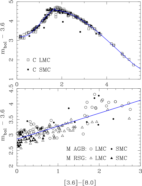
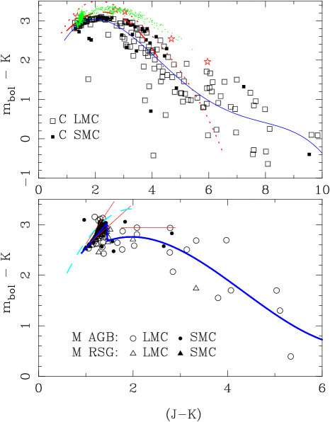
Figure 3: Bolometric correction at 3.6 $\mu$m versus [3.6]$-$[8.0] colour (left) and $K$ versus $J-K$ colour (right) for C stars (top panels) and M stars (bottom panels). The solid dark-blue lines are polynomial fits to the data (see Table 16). See Section 5.2 for an explanation of sources not fitted or plotted. For C stars in the top right panel, red stars indicate models by Nowotny et al. (2013), green dots indicate models by Eriksson (2014), the dotted red line indicates the fit by Kerschbaum et al. (2010), and the dashed red line indicates the fit by Whitelock et al. (2006). For M stars in the lower-right panel, the straight red lines indicate relations ”A”, ”B”, and ”C” from Kerschbaum et al. (2010), valid in the range $1.0<J-K<1.6$, $1.1<J-K<1.95$, and $1.75<J-K<2.9$ mag, respectively. The dashed light blue line indicates the fit by WBF.

5.3 Mass-loss rates

Figure 4 plots MLR as a function of [3.6]$-$[8.0] colour generated from synthetic photometry of the fitted models. It closely resembles the corresponding figure from G09. Generally, redder colours are associated with larger MLRs, as expected. The relations are tight, with no clear dependence on metallicity (assuming that the expansion velocity and gas-to-dust ratio do not depend on metallicity).

Sloan et al. (2008) fitted a line to the logarithm of the MLR as a function of colour for carbon stars. They used a spectroscopically derived colour ([6.4]$-$[9.3]), which closely follows the photometric [5.8]$-$[8] colour (Sloan et al. 2016). However, the older sample did not include targets observed later in the Spitzer mission, which added more sources at the red and blue ends of the colour range. For the carbon stars, the additional sources do not follow a single linear relation. Matsuura et al. (2009) used a three-parameter function based on the inverse of the colour, which adds the necessary curvature. For the carbon stars,

$${\rm\log}\,\dot{M}=-4.080\,-\,\frac{6.531}{([3.6]-[8.0])\,+\,0.941}.$$ (1)

The typical uncertainty in log (MLR) is about 0.22 dex. The three data points with [3.6]$-$[8.0] $\sim$ 6.5 mag and $\log\,\dot{M}>-4$ are excluded, because they have probably evolved off of the C-rich sequence defined by the rest of the sample. Two of these sources appear in the sample of Magellanic carbon-rich objects of Sloan et al. (2014), primarily because their IRS spectra were redder than any of the carbon stars considered by Sloan et al. (2016). The spectra showed no other obvious spectral features associated with post-AGB objects, such as forbidden lines, fullerenes, or polycyclic aromatic hydrocarbons (PAHs). The third source is one of the EROs from the sample by Gruendl et al. (2008), ERO 0518117.

As a group, the observed photometry of these sources suggests that they have begun to evolve off of the AGB, by showing both reduced variability and bluer colours at shorter wavelengths. C stars generally show a tight relation between most infrared colours, so that in most CCDs, they fall along an easily recognisable sequence. However, some of the reddest sources depart from that sequence. For example, several of the EROs have a bluer colour at [3.6]$-$[4.5] than expected from [5.8]$-$[8.0] (Fig. 13 from Sloan et al. 2016). These sources may be deviating from spherical symmetry, allowing some light from the central star to escape via scattering in the poles of the extended envelope. One should keep in mind that our models assume spherical symmetry. Sloan et al. (2016, Fig. 14) also found that the variability of C stars increases to a [5.8]$-$[8.0] colour of $\sim$1.5 mag, but past that colour it decreases. One would expect decreased variability as a star sheds the last of its envelope and departs the AGB.

For the M stars,

$${\rm\log}\,\dot{M}=-4.708\,-\,\frac{2.488}{([3.6]-[8.0])\,+\,0.545}.$$ (2)

The typical uncertainty is about 0.49 dex in $\log\,\dot{M}$, which is larger than for the C stars, due mostly to the apparent split in the relation for AGB stars and red supergiants, with the supergiants usually showing higher MLRs. This relation is not valid at the bluest colours, [3.6]$-$[8] $\lesssim$ 0.1 mag, because the actual MLRs drop to zero much more quickly than the fitted relation indicates.

The major difference with G09 is that the current C-rich models use the optical constants for AMC from Zubko et al. (1996), while G09 used the constants from Rouleau & Martin (1991).

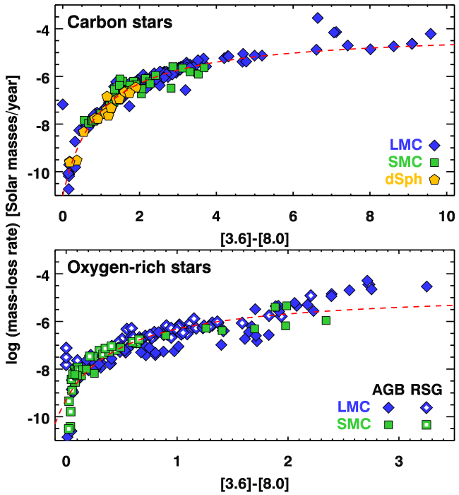
Figure 4: Mass-loss rate versus colour for C stars (top panel), and M stars (bottom panel). The fitted relations are shown as dashed orange curves and are given by equations (1) and (2). The carbon stars include sources from the LMC, SMC, and dwarf spheroidal galaxies.

6 Discussion

6.1 Comparison to other works

6.1.1 Groenewegen et al. (2009)

First we compare the MLRs derived by G09 to the present paper, which includes more photometry for the SED, uses different model atmospheres, and uses improved code for radiative transfer. In addition, the absorption and scattering coefficients have been calculated differently and with different optical constants, with a change in amorphous carbon for the C stars and a change from astronomical silicates derived from observations to silicates measured in the laboratory for M stars.

The ratio of the MLRs for 76 non-foreground (FG) M stars (in the sense of old/new) has a median value of 1.17, with 90% of the ratios in the range 0.6 to 2.7. The M stars show no obvious systematic effects, and the scatter suggests a random fitting error of a factor of two in the MLR.

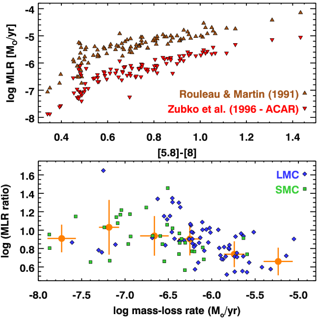
Figure 5: Comparison of the mass-loss rates for carbon stars between the present work and G09. The current work uses optical constants for amorphous carbon from Zubko et al. (1996), while G09 used constants from Rouleau & Martin (1991). Top: A direct comparison for the common sources shows that the new models have much lower MLRs. Bottom: The ratios of the MLRs tend to be approximately nine, although the difference between the models drops for the highest MLRs. The gold data points in the bottom panel are the median values for the log of the MLR ratio in each 0.5-dex bin, plotted against the mean log MLR; the error bars are the formal standard deviations.

The difference between the current models and those of G09 is much more dramatic for the carbon stars, as Figure 5 shows for the 101 sources in common between the two samples. This difference arises primarily from the shift from the optical constants for amorphous carbon from Rouleau & Martin (1991) to the ACAR sample from Zubko et al. (1996). The mean ratio is 8.99, the median is 7.58, and the standard deviation is 5.82. 80% of the sample have a ratio of MLRs between 5.2 and 11.4. The bottom panel of Figure 5 shows that the change in MLR due to the change in optical constants decreases with higher MLR, down to a ratio of 5.0 for the highest mass-loss bin.

A direct comparison of the extinction coefficient of the amorphous carbon grains used in the present work and by G09 (they assumed small grains and ignored scattering) shows that the ratio of opacities is about 9.5 at 1 $\mu$m and 5.4 at 2 $\mu$m, consistent with the trend seen in Fig. 5.

These results reveal the impact of the chosen optical constants for amorphous carbon. The constants from Zubko et al. (1996) produce slightly better fits to the observed spectra, but no compelling reason exists for choosing one set of constants over another. The consequences of this decision are substantial. Boyer et al. (2012) and Matsuura et al. (2013) both estimated the total dust input from AGB stars in the SMC and LMC, but their estimates differed by factors of approximately 8 in the LMC and $\sim$11 in the SMC. In both cases, the estimates by Matsuura et al. were higher, because they used the models by G09 to calibrate the MLRs of their photometric sample, and those models were based on the optical constants from Rouleau & Martin (1991). Boyer et al., on the other hand, used the GRAMS models (Srinivasan et al. 2011), which are based on the ACAR constants from Zubko et al. (1996).

Dust grains with more regular lattice structures should be more efficient absorbers and emitters, because they can function as better antennae. If we can apply that principle to the dust constants, it follows that more graphitic carbon-rich dust will have higher opacities, and thus require less dust mass to explain a given amount of emission and absorption. More amorphous dust would require more mass, and that is consistent with the constants from Rouleau & Martin (1991), the models by G09, and the estimated total dust inputs in the SMC and LMC by Matsuura et al. (2013). On a microscopic level, graphitic grains can be described as purely aromatic sheets of carbon, while more amorphous grains would consist of mixtures of aromatic and aliphatic carbon. The aliphatic/aromatic ratio is thus the key descriptor of the dust. It would be particularly helpful for future laboratory work to explore this ratio in their samples, because we still do not have a way to distinguish what best fits the carbon stars we have observed. And as noted already, this lack of knowledge leads to significant uncertainty in total dust production by carbon stars in nearby galaxies.

6.1.2 Riebel et al. (2012)

We can also compare our results to those of Riebel et al. (2012), who derived MLRs for a sample of $\sim 30\leavevmode\nobreak\ 000$ AGB stars and RSGs in the LMC by fitting up to 12 photometric bands with the GRAMS models. We matched our source list to their LMC targets using a search radius of 1″ and only keeping stars for which they list an error in the MLR of less than 30%. In Fig. 6 we plot the ratio of our dust MLRs (found by dividing the MLR by 200) and theirs. For 130 C stars in common the median of this ratio is 0.46, with 90% of the stars within a factor of 2.7 of this. For 63 M stars (excluding FG objects) the median ratio is 0.17 with 94% within a factor of three of this value.

The difference in MLRs could arise from different inner radii in case of the C stars (see next section) while for the O stars it could be due to the difference in using astronomical silicates versus opacities based on optical constants measured in the laboratory (see Sections 6.1.4 and 6.1.5).

Figure 6: Ratio of dust MLRs found in the present paper and by Riebel et al. (2012). In the top panel the C stars, in the bottom panel the O-rich stars. The lines indicate the mean ratios of 0.46, and 0.17, respectively.

6.1.3 Srinivasan et al. (2011)

Srinivasan et al. (2011) compared their results to G09 and found that their MLRs were a factor 1.7 lower (median value). They related this difference to their use of the optical constants from Zubko et al. (1996), while G09 used the constants from Rouleau & Martin (1991). However, as noted in the previous section, the same change in optical constants reduces the MLRs by a factor of between 5 and 10 for the stars in common between the present work and G09. Thus the differences in methodology must also affect the estimated MLRs.

Table 3 lists the four stars used to calibrate the GRAMS models. They are the C stars TRM 88 and OGLE LMC-LPV-28579 (our identifier is ogle051306), and the M stars HV 5715 and SSTISAGE1C J052206.92-715017.6 (our identifier is sagemcj052206). The table lists the derived luminosities and dust MLRs in the various papers, with the error or range in the parameters when available.

Sargent et al. (2010) and Srinivasan et al. (2010) describe the detailed radiative transfer modelling of the SED and IRS spectrum of the two M stars and C stars, respectively. The same numerical code, optical constants, grain-size distribution, etc., derived in these papers were then used in the generation and validation of the GRAMS model grid (Sargent et al. 2011, Srinivasan et al. 2011), and its application (Riebel et al. 2012, Jones et al. 2012, Srinivasan et al. 2016). Other papers have modelled the SED and/or IRS spectrum using independent methods (e.g. van Loon et al. 1999, G09, Jones et al. 2014).

It is important to note that the estimates for luminosity and MLR by Srinivasan et al. (2011, 2016), Sargent et al. (2011) and Riebel et al. (2012) are based on the same GRAMS model grid. These efforts differed in the details of how the photometric data were gathered and the models were fitted, but they all used models from the same grid. Their estimated luminosities and dust MLRs agree well, although, as discussed below, the work of Jones et al. (2012), which also used the GRAMS model grid, differed more significantly.

Section 6.1.2 quoted median ratios for our dust MLR to those by Riebel et al. of 0.46 for C stars and 0.17 for O stars. Within the errors these ratios are consistent with the values for the individual objects (0.42 and 1.65, respectively, for the C stars TRM 88 and ogle051306, and 0.16 and 0.21 for the two O stars).

However, the present work determines a dust MLR for TRM 88 approximetely eight times lower than G09. This difference cannot be due entirely to the different optical constants. Other differences in the approach by us, G09, and Riebel et al. (2012) must also play a role.

A likely suspect is that the GRAMS models allow for larger temperatures at the inner radius. The GRAMS models are run for a fixed grid of inner radii ($R_{\rm in}$= 1.5, 3, 4.5, 7, 12 $R_{\star}$ for the C-star grid, and 3, 7, 11, and 15 $R_{\star}$ for O-star grid), but only models with corresponding temperatures below 1800 K and 1400 K (respectively) are kept. The present work does not accept condensation temperatures higher than 1200 K. Srinivasan et al. (2011) provide $R_{\rm in}$ or $T_{\rm c}$ for our calibration C stars. For TRM 88, we find an inner radius of 15.6 $R_{\star}$, while Srinivasan et al. find a lower value, 12 $R_{\star}$, which is consistent with the ratio of dust MLR of 0.42 between the present work and the GRAMS grid. For OGLE 051306 we find 14.1 $R_{\star}$, while Srinivasan et al. (2010) find 4.4 $R_{\star}$, a difference due to the temperature at the inner radius, 970 versus 1300 K. If we had adopted that temperature, our MLR would drop by factor of 3.2, and the ratio of our dust MLR compared to Riebel et al. (2012) would decrease from 1.65 to 0.5, or close to the median value.

6.1.4 Jones et al. (2012)

For the O-rich stars HV 5715 and sagemcj052206, Sargent et al. (2010) fitted the SED and IRS spectra, and their results agree well with the GRAMS-based results of Sargent et al. (2011) and Riebel et al. (2012) (see Table 3). The fitting method of Jones et al. (2012), however, led to a much higher estimate of dust MLRs. They also used the GRAMS model grid, but the details of their method differed.

An examination of the 69 M stars in common between Jones et al. (2012) and Riebel et al. (2012) leads to a median ratio in the MLRs of 1.6 (Jones et al. / Riebel et al.), which is not large, but only 35% of the stars lie within a factor of three of the median. Nineteen stars have MLR ratios which differ from the median by a factor of 10 or more, and five differ by a factor of 75 or more. Thus the scatter when considering individual objects is significantly higher, even if the statistical difference for the overall sample is small. As noted above, for 63 M stars in common between Riebel et al. (2012) and the present work, the median ratio (this work / Riebel et al.) in the MLRs is 0.17, with no object with an MLR ratio more than a factor of ten from the median. That difference presents the opposite problem: a reasonable consistency among source-to-source, but a greater shift between the model results overall.

6.1.5 Jones et al. (2014)

Jones et al. (2014) investigated a sample of evolved stars in the LMC by fitting photometry and IRS spectra to a grid of models calculated with the code MODUST (Bouwman et al. 2000). Table 3 shows that for HV 5715 and sagemcj052206, they find much lower dust MLR than Jones et al. (2012), and this result is generally true for the larger sample. The two samples contain 26 stars in common, and the median ratio of the 2014 results to 2012 is 0.13, again with a large scatter; for 30% of the stars the difference exceeds a factor of five. The major difference between the two works is the adopted opacities: Jones et al. (2012) relied on the GRAMS models which use the ‘astronomical silicates’ from Ossenkopf et al. (1992), while Jones et al. (2014) derive the opacities from optical constants measured in the laboratory, as in the present work.

The differences between the dust MLR from Jones et al. (2014) and the present work are relatively small and uniform. For 18 stars in common, the median ratio is 1.65, with all stars within a factor of 2.6 of this value. Because both papers used identical optical constants for amorphous silicates and aluminium oxide, the differences are likely due to the differences in the opacity for iron and the derived (present paper) or adopted (Jones et al. 2014) iron fraction. Differences in the radiative transfer and fitting procedure are likely to have had a smaller effect. We typically find larger iron fractions than adopted by Jones et al. (2014) and hence lower MLRs.

We have calculated the extinction coefficient for warm oxygen-deficient silicates from the astronomical silicates from Ossenkopf et al. (1992) for single-sized grains of 0.15 $\mu$m and compared those to the grains that best fit HV 5715 and sagemcj052206 in the present work. The grains in the present work are larger, and the ratio of opacities at 1 and 2 $\mu$m are 1.5–2.6 and 2–6, respectively, consistent with the differences in MLRs between the present work and most of the works based on the M-star GRAMS grid.

Table 3: Comparison of derived dust MLRs and luminosities for two C stars (TRM 88 and OGLE 051306) and two O stars.

Reference	$L$	$\dot{M}$dust
	($L_{\odot}$)	(10-9 $M_{\odot}$ yr-1)
TRM 88
van Loon et al. (1999)	13300	6.0
G09	7160	16.1
Srinivasan et al. (2011)	11700	3.4
Riebel et al. (2012)	9120 $\pm$ 650	4.92 $\pm$ 0.58
present paper	9403	2.1
OGLE 051306
Srinivasan et al. (2010)	4810, 6580	2.5 (2.4-2.9)
Srinivasan et al. (2011)	6170	2.4
Riebel et al. (2012)	7080 $\pm$ 700	2.12 $\pm$ 0.42
present paper	4740	3.2
HV 5715
Sargent et al. (2010)	36 000 $\pm$ 4000	2.3 (1.1-4.1)
Sargent et al. (2011)	33 000	1.5
Riebel et al. (2012)	33 700 $\pm$ 5960	1.56 $\pm$ 0.43
Jones et al. (2012)	28 800	19.6
Jones et al. (2014)	19 230 $\pm$ 4300	0.63 $\pm$ 0.14
present work	28 200	0.25
sagemcj052206
Sargent et al. (2010)	5100 $\pm$ 500	2.0 (1.1-3.1)
Sargent et al. (2011)	4900	2.1
Riebel et al. (2012)	4820 $\pm$ 670	2.11 $\pm$ 0.44
Jones et al. (2012)	4740	19.6
Jones et al. (2014)	3160 $\pm$ 710	0.68 $\pm$ 0.19
present work	4120	0.45

6.2 Mass-loss and stellar evolution

G09 compared the MLR vs. luminosity diagram with predictions from stellar evolutionary models by Vassiliadis & Wood (1993, hereafter VW) and those using recipes developed by Wagenhuber & Groenewegen (1998) with a Reimers mass-loss law (with multiplicative scaling parameter $\eta=5$ on the AGB). The comparison largely favoured the VW models, vindicating their adopted mass-loss recipe, which is essentially the minimum of the single scattering limit $\dot{M}$$=2.02\cdot 10^{-8}\,L/v_{\rm exp}$, and an empirical relation between $\log\dot{M}$ and $P$. The fundamental-mode period, $P$, is calculated from a period-mass-radius relation (see VW for details).

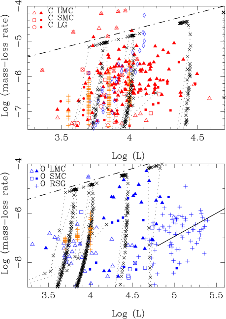
Figure 7: Total MLR versus luminosity for C stars (top panel, red colours) and M stars (bottom panel, blue colours). Objects with Mira-like pulsation amplitudes are plotted with filled symbols; objects with smaller amplitudes with open symbols. An overplotted cross indicates no information on pulsation properties. Orange plus signs in the top panel indicate models by Eriksson et al. (2014) scaled to our adopted dust-to-gas ratio and expansion velocity (see text). Blue diamonds in the top panel indicate a sample of Galactic C Miras (see text). RSGs are plotted as plus signs independent of host galaxy and pulsation amplitude. Orange plus signs in the bottom panel indicate models by Bladh et al. (2015) scaled to our adopted dust-to-gas ratio and expansion velocity (see text). The VW models for LMC metallicity are plotted as crosses connected by the dotted lines for initial masses of 1.5, 2.5, 5.0 and 7.9 $M_{\odot}$, but not every track is visible in every panel. Each cross represents a time interval of 5000 years. The dot-dashed line shows the single scattering limit for a velocity of 10 km s^-1. The solid line is the relation found by Verhoelst et al. (2009) for Galactic RSGs.

Figure 8: Binned version of Fig. 7 for C stars.

Figure 7 shows the relation between MLR and luminosity, with the VW model tracks for LMC metallicity overplotted (the crosses connected with the dotted lines). From the individual evolutionary tracks, a model is plotted every 5000 years. The density of points therefore represents the time spent at a certain position in the diagram. It also explains the ‘excursions’ which are due to the finite probability of catching a star during a thermal pulse or the luminosity dip that follows. Models are plotted for initial masses of 1.5, 2.5, 5.0 and 7.9 $M_{\odot}$, which evolve at increasing luminosity.

The distribution of MLRs for the O-rich AGB stars (in the bottom panel) is similar to that described by G09. They are prominent at lower luminosities, which correspond to lower masses where C stars are less likely to form or will form later during their evolution on the AGB. Oxygen-rich AGB stars are largely absent at intermediate luminosities, which correspond to masses dominated by C stars, and they are prominent at higher masses, where hot-bottom burning inhibits the formation of C stars. Essentially no stars exceed the single-scattering limit. The MLRs of the RSGs scatter around the relation for Galactic RSGs derived by Verhoelst et al. (2009), $\log\dot{M}=-16.4+1.89\log L/L_{\odot}$. The spread is $\sim$2 dex, which is larger than the $\sim$1-1.5 dex scatter in the relation for Galactic RSGs.

The orange plus signs represent the recent dynamical models by Bladh et al. (2015) for M stars with masses of 1 $M_{\odot}$ and solar metallicities. The models are available for 5000, 7000, and 10000 $L_{\odot}$ and cover a range in effective temperatures, piston-velocity amplitudes and seed-particle densities. The plotted MLR is their value scaled to our adopted dust-to-gas ratio and expansion velocity. The differences are significant. The median values in the 56 models of dust-to-gas ratio ($\Psi$) and $v_{\rm exp}$ are 5.8 $\cdot 10^{-4}$ and 10.4 km s^-1, respectively. The difference in $\Psi$ is considerable, and their calculated MLRs are a median 1.1 dex above the scaled values plotted in Figure 7. A comparison to our determinations is difficult because of the difference in metallicity and mass, but the agreement is within an order of magnitude, which is encouraging given the fact that the driving of winds in M stars is a difficult problem (Woitke 2006, Höfner 2008).

The top panel of Figure 7 shows the results for the C stars. The orange plus signs are the results of the dynamical models at solar metallicity by Eriksson et al. (2014). From the 540 models they calculated we show the 193 models which result in a outflow (not all models do), and then those with an expansion velocity larger than 5 km s^-1. The plotted MLR is their value scaled to our adopted dust-to-gas ratio and expansion velocity. This difference is significant. The median values for the 193 models of dust-to-gas ratio ($\Psi$) and $v_{\rm exp}$ are 0.0014 and 23.4 km s^-1, respectively, which differ considerably from our values. Their calculated MLRs lie a median 0.91 dex above the scaled values plotted in Figure 7, and reach and exceed the single-scattering limit (see below).

The different models at a given luminosity are related to differences in the other input parameters like effective temperature, overabundance of carbon, or velocity of the piston at the inner boundary of their models.

Figure 7 also includes Galactic stars (plotted as blue diamonds). The fitting for the Galactic targets was done using different software and dust opacities, which we can expect to lead to differences in derived MLRs (see Sect. 6.1). This sample includes three groups.

Groenewegen et al. (1998) modelled the SEDs and spectra of 42 Galactic carbon-rich Miras. In this case, the spectra were from the Low-Resolution Spectrometer (LRS) aboard the Infrared Astronomical Satellite (IRAS). Miras were chosen so that the period-luminosity relation could be used to estimate their distances, which are always a challenge for evolved stars in the Galaxy. As part of a different (unpublished) investigation, six stars in that sample covering a range of MLRs were fitted with MoD to derive the differences in MLRs, using updated photometry and where possible, spectra from the Short-Wavelength Spectrometer (SWS) aboard the Infrared Space Observatory (ISO). The third group comes from Groenewegen et al. (2016) who modelled some very red Galactic objects with MoD using the same method as in the present paper. That sample included three additional stars overlapping Groenewegen et al. (1998), and two other stars. Thus the Galactic sample consists of 44 stars: 33 taken directly from the models by Groenewegen et al. (1998), nine from that sample based on updated models, and two additional stars.

The median ratio of the MLRs (old/new) is 3.8, and this is largely due to the change in optical constants (Groenewegen et al. 1998 also used the constants from Rouleau & Martin 1991). We have scaled the 33 old models by this median ratio. We have also scaled the MLRs of these stars to an expansion velocity of 10 km s^-1, as adopted in the rest of the sample. The stars follow a close relation which is due to the underlying adopted period-luminosity relation.

Compared to G09, the qualitative description of the comparison has changed. G09 found that only three C stars were slightly above the single-scattering limit, which they considered to be consistent with expectations. In the current picture, a significant number of C stars are above the single-scattering limit by up to a factor of ten. This in itself does not necessarily pose a significant issue. First, the MLRs have large uncertainties (and $\beta$, too, due to the assumed gas-to-dust ratio of 200 and expansion velocity of 10 km s^-1). Second, dynamical models show that $\beta>$ 1 can be reached in realistic models. From a subset of 900 dynamical model atmospheres for carbon stars for solar metallicities from Mattsson et al. (2010), we find that the 98th percentile on $\beta$ is 3.0. In the more recent models by Eriksson et al. (2014), the 98th percentile on $\beta$ is 1.5. From dynamical model atmospheres for subsolar metallicities by Wachter et al. (2008) one might expect the value for $\beta$ to be a factor 2.6 lower in the LMC, i.e. near 0.5-1.

If confirmed, our models show that the artificial cut-off in the VW models at $\beta=1$ may be too conservative. A cut-off (if any) at a larger $\beta$ would result in shorter AGB lifetimes.

Figure 8 presents the results differently, with the MLRs of the C stars binned and averaged for the SMC, LMC, dSph galaxies, and our Galaxy separately. The VW evolutionary tracks suggest that for a given mass, the luminosity evolves by about 0.1 dex on the AGB (Fig. 7), and as a consequence we chose this as the bin size in $\log L$. The MLRs in a luminosity bin are median averaged in $log$ $\dot{M}$ and are plotted in Fig. 8 at the average luminosity of the stars in that bin if a bin includes three or more objects. The error bar indicates the spread in the bins (as 1.5 times the median absolute deviation).

The MLR increases globally with luminosity, as also shown by the models by Eriksson et al. (2014). Any dependence on metallicity remains difficult to assess. The issue of accurate distances (hence luminosities) remains a limiting factor for any Galactic sample. The models in the present work point to a larger dust MLR in the LMC than in the SMC for a given luminosity, but this could also arise from the difference in the underlying populations (see below) and/or differences in expansion velocity.

Groenewegen et al. (2016) determined for the first time the expansion velocity of four C stars in the LMC by detecting the CO J=2-1 transition using the Atacama Large-Millimeter Array (ALMA). All four of these stars are in the present sample: IRAS 05506, IRAS 05125, ERO 0529379, and ERO 0518117. They compared these objects to the closest available analogs in the Galaxy and found that the expansion velocity in the LMC appears to be smaller than in the Galaxy. The key caveat, though, is that the samples are small, and it is difficult to find suitable comparison objects in the two galaxies.

Figure 7 shows clearly that between the LMC and SMC, the stars with the heaviest mass loss are located in the LMC. This result does not appear to result from a bias in the spectroscopic sample observed by the IRS. Plotting colour-magnitude diagrams (CMDs) of photometric samples in the mid-IR reveals more intrinsically red AGB stars in the LMC compared to the SMC (Fig. 5 from Ventura et al. 2016, and references therein). Comparison to models shows that the largest degree of obscuration in the LMC and SMC occurs for stars with an initial mass of 2-3 $M_{\odot}$ and about 1.5 $M_{\odot}$, respectively, a difference which Ventura et al. (2016) attribute to differences in the star formation histories of the two galaxies. Such differences between the populations in the LMC and SMC make it difficult to draw any firm conclusions about how the MLR depends on metallicity.

6.3 A super-AGB star candidate

G09 suggested that MSX SMC 055 (or IRAS 00483$-$7347) is a good candidate for a super-AGB (SAGB) star, based on its high luminosity ($M_{\rm bol}=-8.0$), its very long pulsation period (1749 days) and large pulsation amplitude (1.6 mag peak-to-peak in $I$). Its pulsational properties distinguish it from a luminous RSG. Here we present improved estimates for its parameters.

Groenewegen & Jurkovic (2017) derived a relation between period, luminosity, mass, temperature, and metallicity based on the 5-11 $M_{\odot}$ initial-mass Cepheid models by Bono et al. (2000). For the parameters $P$= 1810 $\pm$ 50 days, $L$= 85350 $\pm$ 8500 $L_{\odot}$, $T_{\rm eff}$= 2500 $\pm$ 100 K, and $Z$= 0.004 $\pm$ 0.001 (errors are adopted), we derive a current pulsation mass of 8.5 $\pm$ 1.6 $M_{\odot}$ with the total error in mass dominated by the error in effective temperature. The simpler period-mass-radius relation for fundamental-mode Mira pulsators from Wood (1990) gives a similar value of 9.2 $\pm$ 1.8 $M_{\odot}$.

The current MLR is estimated to be 4.5 $\cdot 10^{-6}$ $M_{\odot}$ yr^-1, assuming a conservative gas-to-dust ratio of 200. Roman-Duval et al. (2014) estimate a value in the ISM in the SMC of 1200${}^{+1600}_{-420}$ which implies the MLR could be larger by a factor of a few. Lifetimes in the thermal-pulsing phase are short in SAGB stars ($10^{4-5}$ years; e.g. the review by Doherty et al. 2017), but these lifetimes in combination with a MLR that could exceed $10^{-5}$ $M_{\odot}$ yr^-1 indicate that the initial mass of MSX SMC 055 could very well be up to 1 $M_{\odot}$ larger than its current mass.

García-Hernández et al. (2009) observed this and other massive AGB star candidates in the MCs in the optical at high spectral resolution. The source MSX SMC 055 is very rich in rubidium, Rb, with [Rb/Z] $\stackrel{{\scriptstyle>}}{{\sim}}$+1.7, which confirms the activation of the ²²Ne neutron source at the $s$-process site and its massive AGB or SAGB nature. Indeed, by comparing these observations to models, they independently suggested an initial mass of at least 6–7 $M_{\odot}$ for this star.

The most viable SAGB star candidate in the SMC and LMC remains MSX SMC 055.

6.4 The potential of JWST

The James Webb Space Telescope (JWST), due for launch in 2019, provides impressive filter sets on its two imaging instruments, NIRCAM and MIRI, which will enable broadband photometric studies of the evolved stellar population in galaxies out to distances of a few Mpc. At least two published papers have already investigated which filter combinations look to be most useful for distinguishing and characterizing different classes of objects.

Kraemer et al. (2017) examined the sample of SMC objects observed by the IRS, using the spectra to confirm the classifications. They found that the 5.6, 7.7, and 21 $\mu$m filters best separated C-rich from O-rich stars, while the 5.6, 10, and 21 $\mu$m filters best separated young stellar objects (YSOs) from planetary nebulae (PNe). Jones et al. (2017a) performed a similar study using over 1000 sources with IRS spectra in the LMC. They discussed how to discriminate O- and C-rich AGB and post-AGB stars, RSG, Hii regions, PNe and YSOs. Both Kraemer et al. and Jones et al. based their CMDs and CCDs on synthetic photometry using the IRS spectra. Therefore, they were limited in showing diagrams based on MIRI filters. In Appendix C we present synthetic photometry for the sample of almost 400 evolved stars in about 75 filters, including the 29 medium and wide-band filters available with the NIRCAM and MIRI instruments.

Figure 9 gives two examples. The first is a CMD resembling the near-infrared and IRAC [3.6] versus $J$$-$[3.6] diagram shown by G09 (SMC objects have been placed at the distance of the LMC). In this diagram, the dustiest AGB stars show a relatively small spread in F360W magnitude and the reddest objects are predominantly C-rich. The second example is a CCD resembling the [5.8]$-$[8.0] versus [8.0]$-$[24] diagram shown in Fig. 1 which separates O-rich and C-rich very well. Replacing the F1800W filter by F2100W or F2550W yields simililar plots, but for a given integration time and signal-to-noise F1800W is a magnitude more sensitive than F2100W and almost three magnitudes more sensitive than F2550W (Jones et al. 2017a). Thus for AGB stars, we recommend the 5.6, 7.7, and 18 $\mu$m filters to discriminate O-rich from C-rich stars.

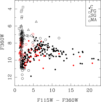
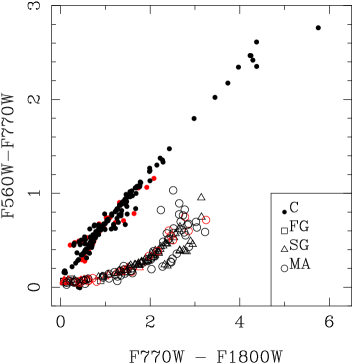
Figure 9: Colour-Magnitude and Colour-Colour diagrams for the LMC (with the SMC stars, plotted in red, shifted to the distance of the LMC) based on synthetic JWST NIRCAM/MIRI magnitudes.

7 Summary and conclusions

We have fitted the SEDs and IRS spectra of almost 400 evolved stars in the SMC and LMC with a dust radiative-transfer model to determine luminosities and (dust) mass-loss rates. The mass-loss rates depend strongly on the adopted opacities (that is, the optical constants, and to a lesser extent the grain shape).

A comparison with results in the literature shows that for M stars the choice of optical constants based on laboratory measurements leads to lower MLRs than those derived from observations (so called, astronomical silicates) as employed in the widely used GRAMS models. When using laboratory-determined optical constants, the iron content that is assumed or derived becomes important and introduces an uncertainty of a factor of two.

For C stars the choice between the widely used optical constants by Rouleau & Martin (1991) and Zubko et al. (1996) introduces a difference in MLR of a factor of approximately five or more. Comparison with the literature suggests that differences in the allowed inner radius in the radiative transfer modelling may also introduce a factor of two uncertainty in the derived MLR.

All of these uncertainties impact the estimates of the total gas and dust return of evolved stars in the MCs (see the references in Section 5.3). The differences in opacities are the greater problem, and the solution lies in a better determination of what circumstellar grains actually look like. While this paper does not offer any solutions to the problem, we hope that we have helped to better frame the problem and its consequences on our understanding of the role played by AGB stars in galactic evolution.

Also of interest are the particular cases of the half-dozen sources with the largest optical depths. They are not the most luminous sources. Groenewegen et al. (2016) and Sloan et al. (2016) discussed their evolutionary status. Evolutionary models using the COLIBRI formalism described by Marigo et al. (2013) (see additional detail by Groenewegen et al. 2016) agree with Ventura et al. (2016) that these stars began their lives with initial masses of 2–3 $M_{\odot}$, but have had their envelope masses reduced to $\stackrel{{\scriptstyle<}}{{\sim}}$1 $M_{\odot}$ through the mass-loss process. The low envelope mass is necessary to explain their long pulsation periods (often longer than 1000 days). Not all of the reddest stars have had their pulsation properties determined, which would clearly be an important contribution. Sloan et al. (2016) noted that the reddest sources showed decreased variability and evidence that radiation from the central star may be escaping the otherwise optically thick dust shell. Both behaviours are consistent with evolution off of the AGB. The unusual blue colours suggest that these stars may also be departing from spherical symmetry, in which case our radiative-transfer models could be underestimating their luminosity. These may be the sources at the very end of their AGB lifetimes, and we need better observational constraints on their geometry and outflows.

Appendix A The sample

Tables 20 and 21 list the samples of C-rich and O-rich stars, with basic information: some common names (as listed by SIMBAD), R.A. and declination in decimal degrees, the identifier used in figures and tables below (where we almost always kept the target name used in the original observation), the adopted pulsation period, the (semi-)amplitude and in which filter. For the oxygen-rich stars a classifier is added (FG=Foreground, SG=Supergiant, MA=M-type AGB-star). These tables are published in its entirety at the CDS; a portion is shown here for guidance regarding its form and content.

The C-stars are listed in order of R.A., but with the stars in the dSph galaxies listed last. For the O-rich stars the foreground objects are listed before the SGs and the AGB stars, and then by R.A. Various criteria have been used to distinguish between foreground, supergiant and O-rich AGB stars; see G09 for details. Compared to G09 only one additional FG object was added HD 269924, which is a K5 star with a significant proper motion. The distinction between SG and MA is sometimes not clear-cut, but our conclusions do not depend on the misclassification of a few objects.

Figure 10 shows one diagnostic that was used, the period-luminosity diagram, with additional information from the pulsation amplitude and colour.

To quantify the impact of misclassifications, we compared our classifications to those from Jones et al. (2012). Of the 46 stars they classified as O-AGB, we classified one as SG, and two as C-rich. Of the 68 stars they classified as RSGs, we classified seven as MA. We also compared our classifications to those from Ruffle et al. (2015), Woods et al. (2011), and Jones et al. (2017b). Of the 18 stars we classified as O-AGB, Ruffle et al. classified two as SG. Of the 21 stars we classified as RSGs, they classified three as MA. Of the 39 stars we classified as O-AGB, Woods et al. (2011) classified 0 as SG. Of the 13 stars we classified as RSGs, they classified zero as MA. Of the 63 stars we classified as O-AGB, Jones et al. (2017b) classified three as SG. Of the 57 stars we classified as RSGs, they classified one as MA. The differences arise mainly because we did not strictly enforce the classic AGB luminosity limit of $M_{\rm bol}=-7.1$ mag. This comparison shows that the probability of misclassification is $\sim$5-10%.

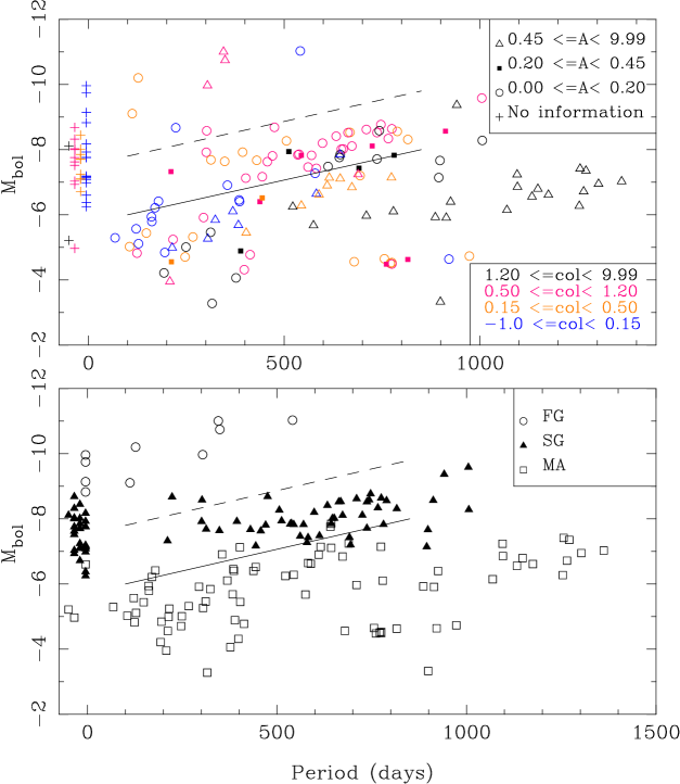
Figure 10: Bolometric magnitude versus pulsation period for the O-rich stars. Stars without periods are plotted as plus signs at negative periods. The solid line indicates the lower luminosity limit for RSGs by WBF, and the dashed line is 1.8 mag brighter. Top panel. The legend indicates the meaning of the symbols in terms of the $I$-band semi-amplitudes ($A$), and [3.6]$-$[8.0] colours. Bottom panel. As top panel, but the objects are identified as foreground objects (open circles), RSG (filled triangles), and AGB stars (open squares).

Table 4: Carbon star sample.

Names	R.A.	Declination	Identifier	Period	Amp (Filter)	Ref.	Remarks
GM 780, MACHO 213.15051.6	8.905250	-73.165583	gm780	611	0.75 ($I$)	1
MSX SMC 029	9.192958	-73.526417	msxsmc029
MSX SMC 091	9.236292	-72.421528	msxsmc091	405	0.57 ($K$)	2
IRAS 00350-7436	9.248792	-74.330639	iras00350
MSX SMC 062, OGLE J004240.89-725705.1	10.670417	-72.951583	msxsmc062	548	0.86 ($I$)	1
MSX SMC 054, MACHO 213.15504.265	10.774699	-73.361268	msxsmc054	390	0.27 ($I$)	1
2MASS J00432649-7326433	10.860361	-73.445350	j004326	327	0.11 ($I$)	1
MSX SMC 044, OGLE J004339.58-731457.1	10.914875	-73.249333	msxsmc044	441	0.60 ($I$)	1
2MASS J00445256-7318258	11.219005	-73.307186	j004452	158	0.06 ($I$)	1
MSX SMC 105, OGLE J004502.14-725223.8	11.258917	-72.873417	msxsmc105	652	0.93 ($I$)	1
MSX SMC 036, OGLE J004553.92-732340.7	11.474750	-73.394750	msxsmc036	555	0.85 ($I$)	1
MSX SMC 014	11.568042	-74.187111	msxsmc014	361	1.05 ($I$)	1
MSX SMC 060, OGLE 004640.46-731646.9	11.668417	-73.279778	msxsmc060	431	0.41 ($I$)	1
MSX SMC 200, smc102.5_195	11.711583	-71.794250	msxsmc200	433	0.36 ($I$)	1
MSX SMC 033, OGLE J004705.55-732132.5	11.773000	-73.359167	msxsmc033	532	0.88 ($I$)	1
SSTISAGEMA J004720.02-724035.1	11.833320	-72.676390	j004720	144	0.05 ($I$)	1
MSX SMC 66, OGLE J004852.51-730856.5	12.218750	-73.149111	msxsmc066	523	0.46 ($I$)	1
2MASS J00485947-7335387	12.247937	-73.594118	irasf00471	687	0.97 ($I$)	1
CV 78, MACHO 212.15907.1	12.265958	-73.088833	cv78	435	0.75 ($I$)	1
RAW 594	12.535420	-72.838940	raw594	140	0.06 ($I$)	1
MSX SMC 163, MACHO 208.16031.578	12.753083	-72.421806	msxsmc163	672	0.87 ($I$)	1
MSX SMC 142, OGLE J005140.46-725728.5	12.918625	-72.958028	msxsmc142	293	0.76 ($I$)	1
MSX SMC 125	12.958690	-72.847080	msxsmc125	458	0.84 ($I$)	1
MSX SMC 162, OGLE J005240.16-724727.3	13.167375	-72.791000	msxsmc162	535	0.51 ($I$)	1
MSX SMC 202, smc102.1_11605	13.292208	-72.198528	msxsmc202	486	0.32 ($I$)	1
MSX SMC 159, OGLE 005422.28-724329.7	13.592830	-72.724940	msxsmc159
LEGC 105, OGLE J005446.85-731337.6	13.695184	-73.227182	legc105	349	0.62 ($I$)	1
OGLE 005450.73-730607.2	13.711458	-73.102028	iso00548	430	0.90 ($I$)	1
OGLE 005454.09-730318.0	13.725417	-73.055028	iso00549	546	0.56 ($I$)	1
RAW 960, OGLE J005554.61-731136.3	13.977620	-73.193470	raw960	315	0.62 ($I$)	1
MSX SMC 209, MACHO 207.16376.687	14.068292	-72.278139	msxsmc209	510	0.80 ($I$)	1
OGLE SMC-SC7 204803	14.073042	-72.451194	s3mc204803	194	0.07 ($I$)	1
IRAS 00554-7351, [GB98] S16	14.266458	-73.587389	iras00554	851	0.83 ($I$)	1
MSX SMC 198, OGLE J005710.97-723059.7	14.295750	-72.516639	msxsmc198	512	0.85 ($I$)	1
MSX SMC 155	14.325625	-72.709778	msxsmc155
2MASS J00572054-7312460	14.335583	-73.212778	iso00573	352	0.60 ($I$)	1
MSX SMC 093, smc107.2_23	14.847333	-73.933611	msxsmc093	463	0.30 ($I$)	1
OGLE 010154.53-725822.1	15.477417	-72.972861	iso01019	337	0.51 ($I$)	1
2MASS J01045315-7204039	16.221485	-72.067774	j010453
MSX SMC 232, OGLE J010603.28-722231.9	16.513750	-72.375611	msxsmc232	460	0.64 ($I$)	1
NGC 419 LE 16, smc110.2_6965	17.004750	-72.888139	ngc419le16	424	0.25 ($I$)	1
NGC 419 IR1, OGLE J010812.92-725243.7	17.054000	-72.878890	ngc419ir1	456	0.43 ($I$)	1
NGC 419 LE 35	17.072880	-72.883720	ngc419le35	173	0.08 ($I$)	1
NGC 419 MIR 1	17.073000	-72.885889	ngc419mir1	738	0.75 ($K$)	3
NGC 419 LE 27, smc110.2_6915	17.086080	-72.881140	ngc419le27	305	0.08 ($I$)	1
NGC 419 LE 18, smc110.2_6943	17.103958	-72.882472	ngc419le18	371	0.07 ($I$)	1
IRAS 04286-6937, MSX LMC 1007	67.125750	-69.513944	iras04286	662	0.56 ($K$)	4
2MASS J04325737-6926331, MSX LMC 1008	68.239083	-69.442528	iras04331	673	0.50 (W2)	5
2MASS J04334368-7009504, MSX LMC 1077	68.432042	-70.164028	iras04340	441	1.08 ($I$)	1
2MASS J04352409-6656493, MSX LMC 1017	68.850417	-66.947028	iras04353	582	0.75 ($K$)	2
2MASS J04364447-7242010, MSX LMC 1067	69.185333	-72.700278	iras04375	246	0.50 (W2)	5
IRAS 04374-6831, MSX LMC 1042	69.344667	-68.417583	iras04374	639	0.71 ($K$)	4
2MASS J04425732-7012257, MSX LMC 1075	70.738875	-70.207167	iras04433	486	0.87 ($I$)	1
2MASS J04462712-6847469	71.613042	-68.796361	sagemcj044627	389	0.91 ($I$)	1
MSX LMC 1120, lmc141.5_9241	71.817042	-68.407111	msxlmc1120	639	0.83 ($I$)	1
IRAS 04496-6958, MSX LMC 1130	72.327000	-69.887361	iras04496	721	0.21 ($I$)	1
MSX LMC 1128	72.668917	-68.971972	msxlmc1128	442	0.68 ($I$)	1

Table 5: M-star sample.

Names	R.A.	Declination	Identifier	Period	Amp (F)	Ref.	Remarks
WOH G 17, MSX LMC 1150	69.848708	-73.184111	wohg17	127	0.13 ($V$)	12	FG
MSX LMC 1212	73.384667	-69.021500	msxlmc1212				FG
RS Men, IRAS 05169-7350, MSX LMC 412	78.921917	-73.787139	rsmen	304	0.53 ($K$)	16	FG
$[$W60$]$ D29, MSX LMC 819	82.997208	-66.644056	w60d29				FG
HD 269788, MSX LMC 778	83.723625	-68.777639	hd269788				FG
MSX LMC 946	84.584292	-69.625639	msxlmc946	112	0.14 ($I$)	15	FG
HD 269924	84.705500	-69.451778	hd269924				FG
MSX LMC 1677, IRAS 06013-6505	90.365833	-65.089750	msxlmc1677	345	2.39 ($V$)	15	FG
HD 271832, MSX LMC 1687, IRAS 06045-6722	91.106208	-67.388444	hd271832	541	0.09 ($V$)	15	FG
MSX LMC 1686, VV Dor, HV 12249	91.699125	-66.803472	msxlmc1686	349	3.01 ($V$)	15	FG
MSX SMC 067, HV 11262	11.903667	-73.078917	msxsmc067				SG
$[$M2002$]$ SMC 10889	12.112583	-73.203417	smc010889				SG
$[$M2002$]$ SMC 11709	12.193000	-73.472417	smc011709				SG
PMMR24, MACHO 212.15903.1	12.215904	-73.377739	pmmr24	430	0.15 ($V$)	15	SG
MSX SMC 096	12.526667	-73.469750	msxsmc096				SG
MSX SMC 109	12.873625	-73.178944	msxsmc109				SG
MSX SMC 168, HV 1652	13.861458	-72.598931	msxsmc168				SG
2MASS J00561387-7227324	14.057833	-72.459028	s3mc203963				SG
2MASS J00561455-7227425	14.060625	-72.461806	s3mc204111				SG
NGC 330 ARP 17	14.079250	-72.468972	s3mc205104				SG
$[$M2002$]$ SMC 46662	14.895872	-72.068463	smc046662	394	0.12 ($V$)	15	SG
$[$M2002$]$ SMC 52334	15.475667	-71.871889	smc052334				SG
PMMR 132	15.516875	-72.436389	pmmr132				SG
$[$M2002$]$ SMC 55188	15.760263	-72.031403	smc055188	544	0.32 ($I$)	1	SG
PMMR 141	15.767833	-72.570305	pmmr141				SG
$[$M2002$]$ SMC 55681	15.804138	-72.157312	smc55681				SG
PMMR 145	15.814084	-72.670111	pmmr145				SG
HV 11464	16.039543	-72.837717	hv11464				SG
$[$M2002$]$ SMC 60447	16.221182	-72.796967	masseysmc60447				SG
HV 2084	17.409256	-73.333940	msxsmc149	737	0.48 ($V$)	15	SG
$[$M2002$]$ SMC 83593	22.641504	-73.311579	smc083593	506	0.47 ($V$)	15	SG
2MASS J04471864-6942205	71.827708	-69.705722	sagemcj044718				SG
HV 2236, MSX LMC 1132	72.343583	-69.409556	hv2236	301	0.18 ($V$)	18	SG
HV 11423	15.229798	-71.631369	hv11423	668	0.34 ($V$)	15	SG
GV 60, WOH S 60, iras 04537-6922	73.378667	-69.297139	gv60	535	0.21 ($V$)	15	SG
MSX LMC 1189, IRAS 04553-6933	73.762792	-69.486861	msxlmc1189	512	0.23 ($I$)	15	SG
WOH G 64, MSX LMC 1182, IRAS 04553-6825	73.793667	-68.341611	wohg64	941	0.45 ($I$)	1	SG
MSX LMC 1204	73.816833	-69.320000	msxlmc1204	663	0.32 ($V$)	15	SG
MSX LMC 1330	73.840208	-69.787972	msxlmc1330	646	0.30 ($V$)	15	SG
MSX LMC 1318, MACHO 17.2473.8	73.889750	-69.416472	msxlmc1318	561	0.12 ($I$)	1	SG
HV 2255, MSX LMC 1328	74.430458	-70.147306	hv2255	912	0.17 ($K$)	19	SG
MSX LMC 1271, HD 268850	75.589458	-66.110639	msxlmc1271				SG
HV 888, MSX LMC 43, IRAS 05042-6720	76.058875	-67.270639	hv888	1005	0.57 ($V$)	15	SG
MSX LMC 141, HV 894	76.389583	-70.563028	msxlmc141	673	0.33 ($V$)	15	SG
HV 916, MSX LMC 264, IRAS 05148-6730	78.707167	-67.455472	hv916	781	0.12 ($K$)	4	SG
$[$M2002$]$ LMC 116895, HV 5760	79.972065	-69.459315	lmc116895				SG
$[$M2002$]$ LMC 119219	80.098395	-69.557450	lmc119219	895	0.41 ($V$)	15	SG
WOH S 264, IRAS 05247-6941 MSX LMC 461	81.080458	-69.647000	wohs264	1006	0.14 ($B$)	6	SG
$[$M2002$]$ LMC 134383, HV 957	81.436891	-69.080244	lmc134383	457	0.24 ($V$)	15	SG
NGC 1948 WBT 2215, [W60] D4	81.504500	-66.271972	ngc1948wbt2215	223	0.34 ($V$)	18	SG
MSX LMC 549	81.547292	-66.203083	msxlmc549	633	0.38 ($B$)	6	SG
MSX LMC 575	81.592417	-66.357917	msxlmc575	816	0.06 ($V$)	15	SG
MSX LMC 589, $[$W60$]$ A2	81.644958	-68.861111	msxlmc589				SG
HV 963, MSX LMC 567	81.893083	-66.891667	hv963	570	0.68 ($V$)	15	SG
HV 2551	81.910834	-69.478917	hv2551	348	0.13 ($V$)	15	SG

Appendix B Mass-loss rates, luminosities, and fits to the SEDs

Tables 22 and 23 list the parameters of the models which best fit the observed data. These include the identifier, information on the atmospheric model used (effective temperature, $\log g$, and for the C stars, C/O ratio), grain size and dust type, luminosity, dust optical depth in the $V$-band, mass-loss rate, whether $\tau$ was fitted (1) or fixed (0), $T_{\rm c}$, whether $T_{\rm c}$ was fitted or fixed, the slope of the denisity law, whether $p$ was fitted or fixed, outer radius (in units of inner radius), and the reduced $\chi^{2}$. These tables are published in its entirety at the CDS; a portion is shown here for guidance regarding its form and content.

The reduced chi-square value is given for reference only. There is a large range in values, and sometimes the values are far larger than unity. This is in part related to the construction of the SED and the available photometery (and error) which can be very different across sources, and the role of variability.

Figures 11 and 2 show the best-fitting models, and give a subjective indication of the quality of the fits. The top panel shows the observed SED and IRS spectrum and the fitted model on an absolute scale, while the bottom panel shows the IRS spectrum and the model (the blue line), scaled to a quasi-continuum point based on the average flux in the 6.35–6.55 $\mu$m region. Horizontal lines near the bottom indicate wavelength regions excluded from the fit.

These figures are vavailable in the online version of the paper. Only some examples are shown here for guidance regarding its form and content.

Table 6: Fit results of the C-star sample.

Identifier	$T_{\rm eff}/\log g/$(C/O)	grain size and type	$L$	$\tau_{0.5}$	$\dot{M}$	f	$T_{\rm c}$	f	$p$	f	$R_{\rm out}$	$\chi^{2}$
	(K/-/-)		($L_{\odot}$)		($M_{\odot}$ yr-1)		(K)				($\cdot 10^{3}$)
gm780	3100/+000/0140	a0.15 zubko100 Pitm10 Hofm0	20019	1.849e+00	1.09e-07	1	1200	0	2.00	0	17	153
msxsmc029	3600/+000/0140	a0.10 zubko100 Pitm0 Hofm0	4984	1.950e+01	1.26e-06	1	676	1	1.53	1	4	53
msxsmc091	2600/+000/0140	a0.15 zubko100 Pitm5 Hofm0	6975	3.345e+00	1.16e-07	1	1200	0	2.00	0	8	350
iras00350	4000/+000/0140	a0.15 zubko100 Pitm0 Hofm10	56665	2.585e+00	1.84e-07	1	1037	1	1.41	1	9.9	83
msxsmc062	2600/+000/0140	a0.15 zubko100 Pitm5 Hofm0	16243	5.523e+00	4.90e-07	1	997	1	2.00	0	8	1149
msxsmc054	2600/+000/0140	a0.15 zubko100 Pitm10 Hofm0	6632	1.071e+01	8.10e-07	1	1016	1	2.24	1	8	551
j004326	3100/+000/0140	a0.15 zubko100 Pitm5 Hofm0	4644	9.571e-01	2.50e-08	1	1200	0	2.00	0	10	228
msxsmc044	3000/+000/0140	a0.15 zubko100 Pitm5 Hofm0	16310	3.220e+00	1.76e-07	1	1200	0	2.00	0	0.037	1945
j004452	2600/+000/0140	a0.15 zubko100 Pitm0 Hofm0	9195	2.697e+00	3.21e-07	1	590	1	1.52	1	10	43
msxsmc105	2600/+000/0140	a0.15 zubko100 Pitm5 Hofm0	7900	6.711e+00	5.94e-07	1	871	1	2.00	0	8	181
msxsmc036	2600/+000/0140	a0.15 zubko100 Pitm5 Hofm0	4634	7.851e+00	4.94e-07	1	902	1	2.00	0	8	707
msxsmc014	3000/+000/0140	a0.15 zubko100 Pitm0 Hofm0	9922	3.608e+01	2.22e-06	1	1200	0	2.13	1	8	435
msxsmc060	2600/+000/0140	a0.15 zubko100 Pitm5 Hofm0	16513	9.044e+00	3.11e-07	1	1200	0	1.60	1	8	249
msxsmc200	3400/+000/0140	a0.15 zubko100 Pitm0 Hofm0	6763	6.000e+00	2.70e-07	1	1200	0	2.21	1	8	394
msxsmc033	2600/+000/0140	a0.15 zubko100 Pitm5 Hofm0	18992	7.168e+00	6.32e-07	1	1200	0	2.38	1	0.037	502
j004720	3500/+000/0140	a0.15 zubko100 Pitm50 Hofm0	16541	2.084e-01	1.45e-08	1	1200	0	2.00	0	17	239
msxsmc066	3400/+000/0140	a0.15 zubko100 Pitm5 Hofm0	17718	7.222e+00	7.87e-07	1	1200	0	2.66	1	8	672
irasf00471	3100/+000/0140	a0.15 zubko100 Pitm5 Hofm0	30455	8.648e+00	6.26e-07	1	1200	0	1.91	1	8	411
cv78	4000/+000/0140	a0.15 zubko100 Pitm5 Hofm0	10007	8.958e-01	4.00e-08	1	1200	0	2.00	0	22	20102
raw594	3300/+000/0140	a0.15 zubko100 Pitm5 Hofm0	4257	6.472e-01	1.63e-08	1	1200	0	2.00	0	10	208
msxsmc163	2600/+000/0140	a0.15 zubko100 Pitm10 Hofm0	11881	6.543e+00	4.27e-07	1	1083	1	2.00	0	8	132
msxsmc142	3300/+000/0140	a0.15 zubko100 Pitm5 Hofm0	4552	2.830e+00	7.95e-08	1	1238	1	2.00	0	0.018	261
msxsmc125	3200/+000/0140	a0.15 zubko100 Pitm5 Hofm0	14932	3.130e+00	1.61e-07	1	1200	0	2.00	0	5	593
msxsmc162	3200/+000/0140	a0.15 zubko100 Pitm5 Hofm0	13166	2.417e+00	1.14e-07	1	1200	0	2.00	0	4	1901
msxsmc202	3100/+000/0140	a0.15 zubko100 Pitm0 Hofm0	14328	1.968e+00	9.08e-08	1	1200	0	2.00	0	0.25	592
msxsmc159	2600/+000/0140	a0.15 zubko100 Pitm5 Hofm0	6512	1.085e+01	3.06e-07	1	1200	0	1.76	1	8	358
legc105	3100/+000/0140	a0.15 zubko100 Pitm0 Hofm0	7739	2.564e+00	8.84e-08	1	1200	0	2.00	0	14	717
iso00548	3400/+000/0140	a0.15 zubko100 Pitm5 Hofm0	11573	5.091e+00	3.53e-07	1	1200	0	2.37	1	12	237
iso00549	3400/+000/0140	a0.15 zubko100 Pitm5 Hofm0	9226	7.886e+00	4.49e-07	1	1105	1	2.00	0	8	728
raw960	3100/+000/0140	a0.15 zubko100 Pitm5 Hofm0	6587	8.716e-01	2.70e-08	1	1200	0	2.00	0	26	368
msxsmc209	2900/+000/0140	a0.15 zubko100 Pitm5 Hofm0	15302	7.203e+00	4.23e-07	1	1173	1	2.00	0	8	1380
s3mc204803	3200/+000/0140	a0.15 zubko100 Pitm5 Hofm0	7394	3.348e-01	1.08e-08	0	1200	0	2.00	0	13	163
iras00554	2600/+000/0140	a0.15 zubko100 Pitm5 Hofm0	23066	1.418e+01	2.56e-06	1	829	1	2.00	0	8	2430
msxsmc198	3400/+000/0140	a0.15 zubko100 Pitm5 Hofm0	7996	5.591e+00	2.08e-07	1	1249	1	2.00	0	8	638
msxsmc155	3400/+000/0140	a0.15 zubko100 Pitm0 Hofm0	8814	1.985e+01	1.09e-06	1	1200	0	2.13	1	8	894
iso00573	3200/+000/0140	a0.15 zubko100 Pitm5 Hofm0	6535	1.777e+00	5.78e-08	1	1200	0	2.00	0	15	289
msxsmc093	2600/+000/0140	a0.15 zubko100 Pitm5 Hofm0	7976	2.291e+00	8.24e-08	1	1200	0	2.00	0	23	340
iso01019	3400/+000/0140	a0.15 zubko100 Pitm5 Hofm0	6161	4.968e+00	2.84e-07	1	1200	0	2.54	1	12	245
j010453	2900/+000/0140	a0.15 zubko100 Pitm0 Hofm0	4514	2.951e+01	1.57e-06	1	997	1	2.00	0	8	121
msxsmc232	3200/+000/0140	a0.15 zubko100 Pitm5 Hofm0	6629	6.875e+00	2.55e-07	1	1200	0	2.00	0	8	498
ngc419le16	3100/+000/0140	a0.15 zubko100 Pitm5 Hofm0	5010	2.321e+00	6.66e-08	1	1200	0	2.00	0	16	439
ngc419ir1	2600/+000/0140	a0.15 zubko100 Pitm5 Hofm0	11990	6.016e+00	4.19e-07	1	1200	0	2.40	1	8	721
ngc419le35	3100/+000/0140	a0.15 zubko100 Pitm5 Hofm0	7050	4.350e-01	1.36e-08	0	1200	0	2.00	0	17	46
ngc419mir1	2600/+000/0140	a0.15 zubko100 Pitm5 Hofm10	8083	4.707e+01	2.32e-06	1	1200	0	1.87	1	8	257
ngc419le27	3200/+000/0140	a0.15 zubko100 Pitm5 Hofm0	6846	4.350e-01	1.35e-08	0	1200	0	2.00	0	17	70
ngc419le18	3200/+000/0140	a0.15 zubko100 Pitm5 Hofm0	5616	4.736e-01	1.34e-08	1	1200	0	2.00	0	19	1027
iras04286	3400/+000/0140	a0.15 zubko100 Pitm5 Hofm0	12136	1.327e+01	4.34e-07	1	1200	0	1.61	1	8	630
iras04331	3300/+000/0140	a0.15 zubko100 Pitm5 Hofm20	8380	2.180e+01	3.12e-06	1	826	1	2.00	0	8	256
iras04340	4750/+000/xxxx	a0.15 zubko100 Pitm10 Hofm0	6409	8.110e+00	5.06e-07	1	1100	0	2.01	1	0.037	109
iras04353	2600/+000/0140	a0.15 zubko100 Pitm5 Hofm15	6902	1.638e+01	1.52e-06	1	869	1	1.87	1	8	837
iras04375	2600/+000/0140	a0.15 zubko100 Pitm5 Hofm10	7257	1.454e+01	1.73e-06	1	794	1	1.96	1	8	269
iras04374	2600/+000/0140	a0.15 zubko100 Pitm5 Hofm0	12159	1.661e+01	1.39e-06	1	1004	1	2.00	0	8	567
iras04433	2600/+000/0140	a0.30 zubko100 Pitm10 Hofm0	7719	5.620e+00	4.71e-07	1	1200	0	2.12	1	8	244
sagemcj044627	2600/+000/0140	a0.15 zubko100 Pitm10 Hofm0	5325	2.993e+00	9.33e-08	1	1200	0	2.00	0	8	374
msxlmc1120	3100/+000/0140	a0.30 zubko100 Pitm5 Hofm0	15377	5.584e+00	6.07e-07	1	1006	1	1.74	1	8	2170
iras04496	2600/+000/0140	a0.15 zubko100 Pitm0 Hofm0	38738	4.527e+00	2.38e-07	1	1200	0	1.66	1	0.40	494

Table 7: Fit results of the M-star sample.

Identifier	$T_{\rm eff}/\log g$	grain size and type	$L$	$\tau_{0.5}$	$\dot{M}$	f	$T_{\rm c}$	f	$p$	f	$R_{\rm out}$	$\chi^{2}$
	(K/-)		($L_{\odot}$)		($M_{\odot}$ yr-1)		(K)				($\cdot 10^{3}$)
wohg17	3300/+0.5	a0.10 Oliv70 AlOx30 Fe30	932967	1.201e-01	2.84e-07	1	1000	0	2.00	0	13	504
msxlmc1212	3900/+0.5	a0.20 Oliv40 AlOx60 Fe1	262501	1.000e-04	1.14e-10	0	1000	0	2.00	0	13	98
rsmen	2500/+0.0	a0.10 Oliv60 AlOx40 Fe30	752101	2.044e-01	4.37e-07	1	1000	0	2.00	0	13	492
w60d29	3800/+0.5	a0.20 Oliv90 AlOx10 Fe30	350174	1.000e-04	8.50e-11	0	1000	0	2.00	0	13	218
hd269788	4250/+0.0	a0.20 Oliv40 AlOx60 Fe3	611699	3.000e-03	8.67e-09	0	760	1	2.00	0	13	4010
msxlmc946	3200/+0.5	a0.10 Oliv50 AlOx50 Fe30	339561	4.252e-02	6.53e-08	1	1000	0	2.00	0	13	51
hd269924	3600/+0.0	a0.10 Oliv40 AlOx60 Fe3	745922	1.000e-03	3.69e-09	0	1000	0	2.00	0	13	4892
msxlmc1677	2700/+0.0	a0.10 Oliv90 AlOx10 Fe30	1952457	6.687e-01	2.05e-06	1	1000	0	2.00	0	13	1315
hd271832	3400/+0.0	a0.50 Oliv80 AlOx20 Fe3	1997701	1.391e-03	4.90e-09	1	1000	0	2.00	0	13	2553
msxlmc1686	2500/+0.0	a0.20 Oliv70 AlOx30 Fe30	1532676	2.973e-01	4.86e-07	1	1000	0	2.00	0	13	270
msxsmc067	3500/+0.0	a0.10 Oliv50 AlOx50 Fe30	143486	1.067e-02	1.12e-08	1	1000	0	2.00	0	13	196
smc010889	3700/+0.5	a0.10 Oliv70 AlOx30 Fe30	184822	5.192e-02	6.01e-08	1	1000	0	2.00	0	10	697
smc011709	3800/+0.5	a0.20 Oliv40 AlOx60 Fe30	114473	1.000e-02	9.16e-09	0	825	1	2.00	0	10	47
pmmr24	3800/+0.5	a0.50 Oliv60 AlOx40 Fe30	90740	9.816e-02	6.28e-08	1	1000	0	2.00	0	10	52
msxsmc096	3700/+0.5	a0.50 Oliv60 AlOx40 Fe30	107095	4.938e-02	3.35e-08	1	1000	0	2.00	0	13	76
msxsmc109	3800/+0.5	a0.10 Oliv90 AlOx10 Fe30	122980	1.344e-01	1.21e-07	1	1000	0	2.00	0	13	245
msxsmc168	3800/+0.5	a0.10 Oliv90 AlOx10 Fe30	93615	5.390e-02	4.21e-08	1	1000	0	2.00	0	13	320
s3mc203963	3900/+0.5	a0.20 Oliv40 AlOx60 Fe1	24445	1.289e-03	4.49e-10	0	1000	0	2.00	0	13	160
s3mc204111	4000/+0.0	a0.20 Oliv50 AlOx50 Fe30	57989	3.000e-03	1.25e-09	0	1000	0	2.00	0	13	7
s3mc205104	4000/+0.0	a0.20 Oliv40 AlOx60 Fe1	27422	1.000e-04	3.74e-11	0	1000	0	2.00	0	13	17
smc046662	3600/+0.5	a0.10 Oliv60 AlOx40 Fe30	113944	3.694e-02	3.42e-08	1	1000	0	2.00	0	10	269
smc052334	3700/+0.5	a0.10 Oliv60 AlOx40 Fe30	97741	1.352e-02	1.18e-08	1	1000	0	2.00	0	10	70
pmmr132	3800/+0.5	a0.20 Oliv70 AlOx30 Fe30	47998	9.110e-05	3.09e-11	0	1000	0	2.00	0	13	442
smc055188	3300/+0.5	a0.50 Oliv100 AlOx0 Fe30	104318	2.131e-01	1.38e-07	1	1000	0	2.00	0	10	218
pmmr141	3700/+0.5	a0.20 Oliv50 AlOx50 Fe30	98039	7.126e-03	3.68e-09	1	1000	0	2.00	0	13	82
smc55681	3800/+0.5	a0.10 Oliv70 AlOx30 Fe30	93022	6.387e-02	5.36e-08	1	1000	0	2.00	0	10	380
pmmr145	4000/+0.0	a0.20 Oliv100 AlOx0 Fe30	52487	5.000e-04	1.64e-10	0	1000	0	2.00	0	13	134
hv11464	3900/+0.5	a0.20 Oliv50 AlOx50 Fe30	55012	1.000e-02	7.15e-09	0	780	1	2.00	0	13	101
masseysmc60447	3800/+0.5	a0.50 Oliv50 AlOx50 Fe30	56568	1.770e-02	8.78e-09	1	1000	0	2.00	0	13	85
msxsmc149	3700/+0.5	a0.20 Oliv80 AlOx20 Fe30	198288	2.661e-01	1.76e-07	1	1000	0	2.00	0	13	416
smc083593	3600/+0.5	a0.10 Oliv80 AlOx20 Fe30	157236	7.268e-02	7.31e-08	1	1000	0	2.00	0	10	200
sagemcj044718	3600/+0.5	a0.10 Oliv60 AlOx40 Fe30	37506	3.201e-02	1.70e-08	1	1000	0	2.00	0	13	58
hv2236	3400/+0.0	a0.10 Oliv95 AlOx5 Fe10	113624	8.817e-01	8.13e-07	1	1000	0	2.00	0	13	716
hv11423	3700/+0.5	a0.10 Oliv80 AlOx20 Fe30	199246	7.809e-02	9.06e-08	1	1000	0	2.00	0	10	652
gv60	3600/+0.5	a0.20 Oliv80 AlOx20 Fe10	105755	5.856e-01	5.30e-07	1	773	1	2.00	0	13	115
msxlmc1189	3500/+0.5	a0.10 Oliv100 AlOx0 Fe30	115869	1.285e+00	1.75e-06	1	800	0	2.00	0	13	198
wohg64	3500/+0.0	a0.10 Oliv70 AlOx30 Fe10	432190	1.732e+01	3.55e-05	1	896	1	1.60	0	0.1	91695
msxlmc1204	3500/+0.0	a0.10 Oliv95 AlOx5 Fe30	198164	1.015e-01	1.85e-07	1	778	1	2.00	0	13	663
msxlmc1330	3400/+0.5	a0.10 Oliv80 AlOx20 Fe10	123820	6.978e-01	7.22e-07	1	1000	0	2.00	0	13	467
msxlmc1318	3200/+0.5	a0.50 Oliv70 AlOx30 Fe30	74948	3.013e-01	2.70e-07	1	800	0	2.00	0	13	163
hv2255	3500/+0.0	a0.10 Oliv90 AlOx10 Fe10	206364	6.201e-01	1.30e-06	1	800	0	2.00	0	13	1061
msxlmc1271	3400/+0.0	a0.20 Oliv70 AlOx30 Fe30	78591	5.075e-01	2.02e-07	1	1000	0	2.00	0	13	95
hv888	3500/+0.5	a0.50 Oliv70 AlOx30 Fe3	526751	2.736e-01	4.76e-07	1	1044	1	2.00	0	13	13598
msxlmc141	3600/+0.5	a0.10 Oliv80 AlOx20 Fe10	135417	5.272e-01	6.10e-07	1	1000	0	2.00	0	13	738
hv916	3400/+0.5	a0.20 Oliv90 AlOx10 Fe30	104646	1.555e+00	6.95e-07	1	1000	0	2.00	0	13	787
lmc116895	3800/+0.5	a0.20 Oliv80 AlOx20 Fe30	124490	1.014e-01	1.01e-07	1	758	1	2.00	0	10	138
lmc119219	3900/+0.5	a0.20 Oliv95 AlOx5 Fe30	55661	1.100e+00	4.04e-07	1	1000	0	2.00	0	10	363
wohs264	3400/+0.5	a0.20 Oliv90 AlOx10 Fe30	158954	1.249e+00	8.71e-07	1	912	1	2.00	0	13	161
lmc134383	3500/+0.5	a0.10 Oliv90 AlOx10 Fe30	87053	2.377e-01	2.79e-07	1	800	0	2.00	0	10	349
ngc1948wbt2215	3500/+0.0	a0.20 Oliv40 AlOx60 Fe30	227669	1.611e-02	2.30e-08	1	830	1	2.00	0	13	79
msxlmc549	3200/+0.5	a0.10 Oliv90 AlOx10 Fe30	178966	3.693e-01	3.51e-07	1	1000	0	2.00	0	13	565
msxlmc575	3800/+0.5	a0.20 Oliv70 AlOx30 Fe30	163654	4.616e-02	3.78e-08	1	893	1	2.00	0	13	29
msxlmc589	3900/+0.5	a0.50 Oliv70 AlOx30 Fe30	230016	2.711e-01	2.88e-07	1	1000	0	2.00	0	13	1933
hv963	3700/+0.5	a0.50 Oliv80 AlOx20 Fe30	104486	2.945e-01	3.91e-07	1	758	1	2.00	0	13	107
hv2551	3600/+0.5	a0.10 Oliv80 AlOx20 Fe30	87885	6.232e-02	4.67e-08	1	1000	0	2.00	0	13	168
hv2561	3700/+0.5	a0.20 Oliv90 AlOx10 Fe10	216781	4.956e-01	6.68e-07	1	758	1	2.00	0	13	146
hv5870	3600/+0.5	a0.10 Oliv90 AlOx10 Fe10	72629	1.054e+00	8.76e-07	1	1000	0	2.00	0	13	449

Appendix C Synthetic magnitudes

Based on the best-fitting model, magnitudes and fluxes are computed in a large number of filters for every star. The procedure follows that in Groenewegen (2006). The calibration is based on the Vega model of Bohlin (2007) and assumes zero magnitudes in all filters.

The filters that are provided are: Bessell $UBVRI$, 2MASS $JHK$, VISTA $ZYJHK$, WISE 1-4, IRAC $[3.6],[4.5],[5.8],[8.0]$, MIPS $[24],[70],[160]$, Herschel PACS $[70],[110],[170]$, SPIRE $[250],[350],[550]$, Akari N2, N3, N4, S7, S9W, S11, L15, L18W, L24, N60, WS, WL, N160, and generic sub-mm filters at 350, 450, 850 and 1300 $\mu$m.

Of interest may be the magnitudes in a large number of wide and medium band filters from NIRCAM (F070W, F090W, F115W, F150W, F200W, F277W, F356W, F444W, F140M, F162M, F182M, F210M, F250M, F300M, F335M, F360M, F410M, F430M, F460M, F480M) and MIRI (F560W, F770W, F1000W, F1130W, F1280W, F1500W, F1800W, F2100W, F2550W) instruments.

Figures 3 and 4 show the normalized SEDs of four C and O stars, respectively, with the NIRCAM and MIRI filters indicated by the FWHM of the response curves.

Table 8, available at the CDS, shows an example of the synthetic photometry for one star. In the electronic version all filters are listed on one single row per object. All values are in magnitudes, except the three PACS, three SPIRE and four sub-mm filters which are given in $\log F$(mJy). The magnitudes and fluxes can be scaled using the adopted distances (see Section 4) and fitted luminosities (Tables 22 and 23) for each star.

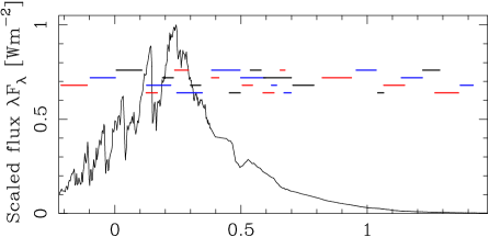
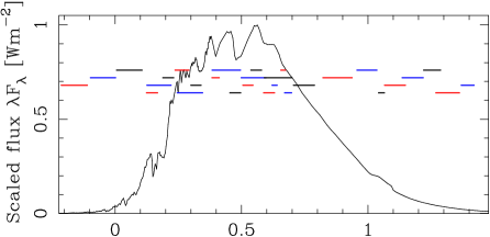
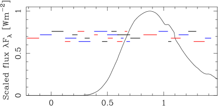
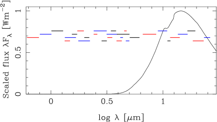
Figure 3: Normalized SEDs of four C stars with little, moderate, strong, and extreme mass-loss rates (NGC 419 LE18, IR1, MIR1, and ERO0518484 from top to bottom). The horizontal bars indicate the FWHM range of 29 NIRCAM and MIRI filters.

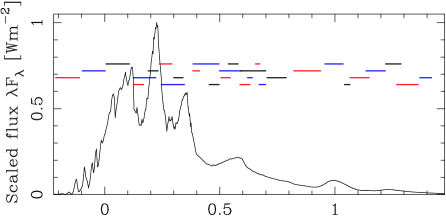
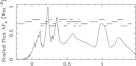
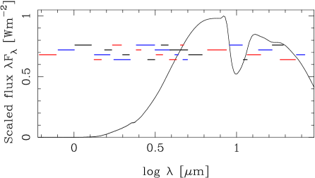
Figure 4: Normalized SEDs of four O stars with little, moderate, strong, and heavy mass-loss rates (MSX LMC 1677, W60 A72, IRAS 05003, and IRAS 05246 from top to bottom). The horizontal bars indicate the FWHM range of 29 NIRCAM and MIRI filters.

Table 8: Synthetic photometry. Example for one object.

Bessell					2MASS			VISTA					WISE
U	B	V	R	I	J	H	K	Z	Y	J	H	K	W1	W2	W3	W4
22.332	20.869	18.654	17.109	15.629	12.970	11.698	11.192	15.057	14.075	12.900	11.726	11.186	10.508	9.314	6.516	5.217
IRAC				MIPS			PACS			SPIRE			Akari
$[3.6]$	[4.5]	[5.8]	[8.0]	[24]	[70]	[160]	70	110	170	250	350	550	N2	N3	N4	S7
10.298	9.419	8.598	7.477	5.123	3.374	2.150	1.551	1.477	1.327	1.096	0.816	0.431	11.075	10.654	9.502	7.760
Akari									JWST
S9	S11	L15	L18W	L24	N60	WS	WL	N160	F070W	F090W	F115W	F150W	F200W	F277W	F356W	F444W
7.206	6.731	5.905	5.591	5.148	3.519	3.107	2.250	2.093	16.604	14.969	13.479	12.190	11.210	11.023	10.333	9.486
JWST
F770W	F1000W	F1130W	F1280W	F1500W	F1800W	F2100W	F2550W	F140M	F158M	F162M	F182M	F210M	F250M	F380M	F300M	F335M
7.555	6.846	6.572	6.303	5.970	5.630	5.347	4.996	12.384	11.832	11.808	11.241	11.172	11.100	9.982	11.147	10.622
JWST						sub-mm				identifier
F360M	F410M	F430M	F460M	F480M	F560W	350	450	850	1300
10.101	9.762	9.519	9.351	9.187	8.619	0.820	0.589	-0.172	-0.666	j004452