Magnetic order and energy-scale hierarchy in artificial spin ice

Henry Stopfel Department of Physics and Astronomy, Uppsala University, Box 516, SE-75120, Uppsala, Sweden Erik Östman Department of Physics and Astronomy, Uppsala University, Box 516, SE-75120, Uppsala, Sweden Ioan-Augustin Chioar Department of Physics and Astronomy, Uppsala University, Box 516, SE-75120, Uppsala, Sweden David Greving Department of Physics, University of Warwick, Coventry, United Kingdom Unnar B. Arnalds Science Institute, University of Iceland, Reykjavik, Iceland Thomas P. A. Hase Department of Physics, University of Warwick, Coventry, United Kingdom Aaron Stein Center for Functional Nanomaterials, Brookhaven National Laboratory, Upton, New York 11973, USA Björgvin Hjörvarsson Department of Physics and Astronomy, Uppsala University, Box 516, SE-75120, Uppsala, Sweden Vassilios Kapaklis Department of Physics and Astronomy, Uppsala University, Box 516, SE-75120, Uppsala, Sweden

In order to explain and predict the properties of many physical systems, it is essential to understand the interplay of different energy-scales. Here we present investigations of the magnetic order in thermalised artificial spin ice structures, with different activation energies of the interacting Ising-like elements. We image the thermally equilibrated magnetic states of the nano-structures using synchrotron-based magnetic microscopy. By comparing results obtained from structures with one or two different activation energies, we demonstrate a clear impact on the resulting magnetic order. The differences are obtained by the analysis of the magnetic spin structure factors, in which the role of the activation energies is manifested by distinct short-range order. This demonstrates that artificial spin systems can serve as model systems, allowing the definition of energy-scales by geometrical design and providing the backdrop for understanding their interplay.

I Introduction

Initially introduced as a playground for the experimental investigation of magnetic frustration effects¹, the area of artificial spin ices has evolved into a vibrant field of research. Using designed structures, collective order and dynamics can be controlled and directly visualized by using, for example, nano-characterization techniques². This approach has motivated experimental investigations of celebrated classical spin models^{3; 4; 5}, some of which display non-conventional and exotic magnetic phases^{6; 7; 8; 9; 10}. Furthermore, given the large freedom in design, new topologies that promote non-conventional emergent order can be manufactured and investigated in thermally-active artificial spin ice structures, allowing the study of their complex energetic manifolds in a superparamagnetic regime ^{11; 12; 13; 14; 15; 16; 17}. A variety of new artificial spin ice systems have been proposed by Morrison et al.¹⁸, with particular attention given to the so-called Shakti lattice, a variation of the square ice geometry. In this lattice, 25% of the square ice lattice elements have been removed and certain pairs of islands merged as depicted in Fig. 1. Theoretical and numerical studies have predicted an emergent magnetic order in the Shakti geometry¹⁹ which retrieves the features of the six-vertex model⁴ on a larger length-scale. This behavior has been demonstrated experimentally by Gilbert et al.²⁰ for the Shakti lattice (SH), as well as for a modified Shakti lattice (mSH).

Given the mesoscopic nature of the structures, different activation energies are expected for the long (T_B1) and short islands (T_B2), resulting in two blocking temperatures of the elements (T ${}_{\rm{B2}}<T_{\rm{B1}}$ ). The presence of two activation energies is therefore expected to influence the eventual magnetic correlations and order in the lattice, since the larger elements could act as a source of quenched disorder. Such disorder would hinder the development of any medium- or long-range magnetic order of the smaller islands, as these become arrested at lower temperatures (T_B2). Whilst the vertex statistics for both the Shakti lattices have been experimentally investigated for a range of inter-island coupling strengths²⁰, the thermally driven kinetics in the modified Shakti lattice were only recently reported¹⁷. Consequently, the impact of the hierarchy of the activation energies on the emergent order has not been addressed to date. In this work, we undertake this task for the particular case of the Shakti and the modified Shakti geometries. Using thermally-active elements, we characterize and compare their final magnetic configurations using identical experimental protocols, highlighting the impact of different activation energies on the obtained magnetic correlations and order.

II Experimental details

II.1 Sample preparation

Refer to caption — Figure 1: A schematic representation of the Shakti (SH) and modified-Shakti (mSH) lattices along with magnetic states representative of each temperature regime, generally defined by the Curie (T_c) and the blocking temperatures (T_B1/B2). Elements in their paramagnetic state are gray, superparamagnetic elements are light-blue and the frozen elements are represented with a magnetic north (blue) and south (red) pole, reflecting their final magnetic orientation. The gray-scale images to the left are representative PEEM-XMCD snapshots obtained at 65 K, the lowest temperature reached during the cooling.

The samples were produced by a post-growth patterning process, applied to a thin film of $\delta$ -doped Palladium (Iron) as described in Pärnaste et al.²¹. A thick bottom layer of Pd (40 nm) is followed by 2.0 mono layers of Fe, defining the nominal Curie-temperature, T ${}_{\rm{C}}=400$ K²¹, as well as the thermally active temperature range for the $\delta$ -doped Pd(Fe). The post-patterning was carried out at the Center for Functional Nanomaterials (CFN), Brookhaven National Laboratory in Upton, New York. A positive high resolution e-Beam resist (ZEP520A) was employed to create a Chromium mask of the nano-structures using e-Beam lithography. The magnetic structures were formed by Argon milling. All investigated structures were produced on the same substrate from the same layer, ensuring identical intrinsic material properties as well as the same thermal history for all the investigated structures. Each array had a spatial dimension of 200 $\times$ 200 $\mu$ m². The lengths of the large and small islands, were chosen to be 1050 nm and 450 nm, respectively, while the width was kept at 150 nm. The lattice spacing between two parallel neighboring short islands was set to 600 nm.

II.2 Thermal protocol

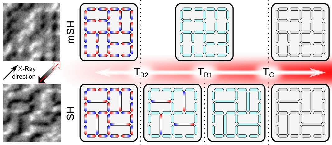
Similar to previous studies^{15; 16}, the thermal protocol involves a gradual cooling from a superparamagnetic state of the elements, towards a completely arrested state at the lowest temperatures. This process is schematically represented in Fig. 1 for both the Shakti and the modified Shakti lattices. Notice the two distinctive stages of the superparamagnetic regime for the Shakti lattice because to the presence of elements with different intrinsic activation energies.

When the temperature is lowered below the Curie temperature (T_c), the elements become magnetic and can be considered as mesospins. The stray field of these islands is resulting in a temperature-dependent magnetostatic coupling. The coupling between the elements has a direct impact on the involved activation energies, biasing the otherwise equally-favoured two magnetic states of the islands. On the lattice scale, this effectively results in a dynamic distribution of blocking temperatures around the intrinsic energy barriers, a distribution whose width depends on the strength of the inter-island interactions.

II.3 Interaction strength and their impact

There are three special cases to be considered: the strong, intermediate and weak coupling limits. In the strong coupling limit, the intrinsic activation energy of the mesospins is much smaller than the inter-island interactions. Consequently, the emergent order will not depend on the differences in the activation energies, but significant effects on the dynamic response cannot be ruled out. In the intermediate coupling limit, the strength of the inter-island couplings is comparable to the intrinsic activation energy of the mesospins. This will give rise to a complex interplay, in which the relation between the activation and interaction energies will dictate both the order and dynamics of the magnetic phases. The individual activation energies depend on the dynamically developing magnetic configurations, for both long- and short-mesospins. In other words, these couplings can yield a strong overlap in the two blocking temperature distributions of the short and long islands. Therefore, the configurations of the long- and the short-mesospins will exhibit different degrees of order, all depending on the relation of the activation and interaction energies. Conversely in the weak coupling limit, the intrinsic activation energies of the long-mesospins are much larger than the inter-island interactions. Around the intrinsic blocking temperature of the long islands (T_B1), the available thermal energy is higher than the energy difference given by any magnetization reversal of the short islands. Therefore the lattice as a whole will be in a disordered state when the long-mesospins freeze (T_B1) and consequently the magnetic orientation of the long elements will be randomly distributed, with no short- or long-range correlations. However, at the blocking temperature for the short-mesospins (T_B2) the inter-island coupling strength can be comparable to their intrinsic activation energies, potentially resulting in a short-range order below T_B2. Thus, having two distinct activation energies is expected to have a significant impact on the emergent order, for both the intermediate and the weak coupling limits. By the same token, the presence of two or more activation energies is expected to have a marginal impact in the strong coupling limit. Here, we focus on the weak coupling limit and, as previously stated, we compare the obtained magnetic order in SH and mSH lattices, ascertaining the impact of the hierarchical relation of inter-element interactions and the activation energies involved.

II.4 Determination of the magnetization direction

The magnetic states were determined as a function of temperature using Photo Emission Electron Microscopy (PEEM) capturing the X-ray Magnetic Circular Dichroism (XMCD) contrast. The experimental studies were performed at the 11.0.1 PEEM3 beamline at the Advanced Light Source, in Berkeley, California, USA. For the SH and mSH lattices the islands were oriented 45 $\degree$ with respect to the incoming X-ray beam, to enable identification of the magnetization direction of all elements in the lattices. For these lattices multiple, partially overlapping, PEEM-XMCD images were acquired and stitched together to form one large image containing over 4000 mesospins for each of the investigated lattices, see Supplementary Materials Fig. 2. The images used for determining the magnetic states were taken at 65 K, far below the Curie-temperature and the blocking temperatures of the short- and long-mesospins. The sampling time ( $t_{s}=300~{}s$ ) required for obtaining a PEEM-XMCD image defines a time window linked to the thermal stability of the mesospins: At the lowest temperatures, all magnetic states are stable (frozen) and the lattice can be imaged for practically arbitrary long times, yielding the same result. However, if the reversal times are much smaller than $t_{s}$ , no magnetic contrast is obtained. This allowed us to ask at which temperature the spins have reversed their magnetization direction within a given time window, thereby providing an estimation on the involved energy scales.

III Results

III.1 Activation energies of the mesospins

Magnetic interactions can affect the inferred activation energies in a profound way. We therefore fabricated two additional lattices consisting of long- and short-mesospins, 1110 nm and 450 nm respectively, in which the distance was large enough to allow us to ignore any effects arising from the interactions between the elements (see Supplementary Materials). The islands were oriented parallel with respect to the incoming X-ray beam, to determine the magnetization direction of the mesospins.

Following the line of argumentation above, we determined that 50% of the short islands reverse their magnetization direction within 300 s at 112 K, while a temperature of 149 K is required for obtaining the same condition for the long islands. The determination of the activation energies is model dependent. Using an expression for the probability of a magnetic element not having altered its magnetization direction after a time period $t_{s}$ ^{22; 16}, as described in the Supplementary Materials, yields a ratio for the activation energies of 0.49(4). This approach provides support for well separated energy-scales, which will be assumed to be the case in the remainder of this communication.

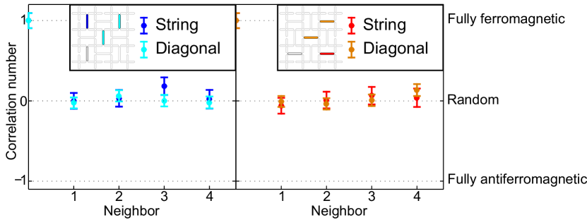
III.2 Correlations of the long-mesospins in the Shakti lattice

The correlations between the long-mesospins were determined from the PEEM-XMCD images recorded at 65 K, after cooling the samples from room temperature with a rate of 1 K/minute. The results from analysis along different directions in the SH lattice are illustrated in Fig. 2. As seen in the figure, no correlations between long-mesospins are observed. The cooling of the sample below the blocking temperature of the short-mesospins does not result in any observed order for the long-mesospins. Because of this, the effective interaction mediated by the short-mesospins must be much smaller than the activation energy of the long-mesospins.

III.3 Magnetic order on the vertex-level

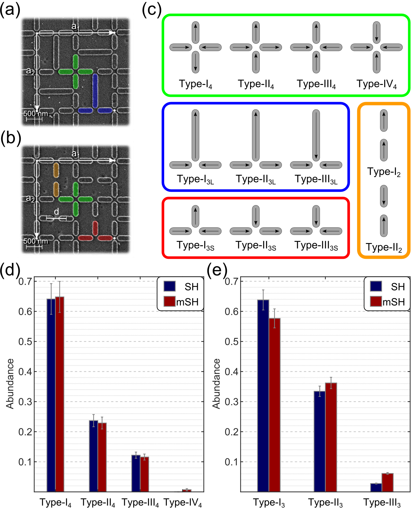
Having established the randomness of the magnetic states of the long-mesospins in the Shakti lattice, we now turn our attention to the overall magnetic order established within the SH and mSH lattices. For square ice related geometries, a commonly-employed tool for characterizing the obtained magnetic state is the determination of populations of the various types of vertex configurations. The different vertex types for both the SH and the mSH lattices are illustrated in Fig. 3(a)-(c). In the nomenclature used here, a roman numeral denotes the vertex type along with a subscript representing the number of mesospins forming the vertex. As an example, I₄ represents four elements forming a Type-I vertex. The mSH lattice has an additional degree of freedom as compared to the SH lattice, arising from the two-fold coordinated vertex having two possible states: Type-I₂ and Type-II₂.

The vertex statistics obtained for the three- and four-fold coordinated vertices are presented in Fig. 3(d) and 3(e), respectively. Comparing the abundance of the different states with published data from Gilbert et al.²⁰, we can again confirm that our results are representative for the weak coupling regime, as $\it{e.g.}$ the previous works on ASI structures^{12; 16}. Notice that these vertex statistics do not display a significant difference between the common vertex states of the SH and mSH lattices, similar to previous reports²⁰. This implies that the final vertex populations are independent of the presence of the long islands in the Shakti geometry and the related energy hierarchy. However, the vertex statistics yield only a partial description of the final magnetic state and are insensitive to magnetic order established over spatial extensions larger than the vertex size.

III.4 Beyond the vertex-level

We use the calculated spin structure factor (SSF) to determine correlations beyond nearest neighbours^{7; 8; 10; 23}. This invokes the use of a Fourier transformation of pairwise correlations of the magnetic states in the following form:

I(\mathbf{q})=\frac{1}{N^{2}}\sum_{(i,j=1)}^{N}\mathbf{S}^{\perp}_{i}\cdot\mathbf{S}^{\perp}_{j}\cdot e^{i\mathbf{q}\cdot(\mathbf{r}_{i}-\mathbf{r}_{j})}

(1)

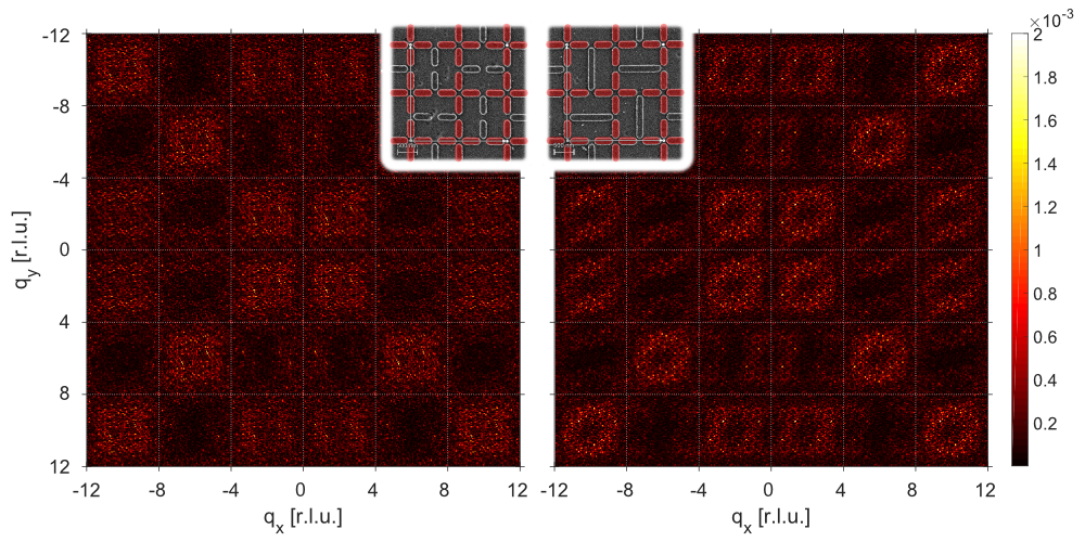
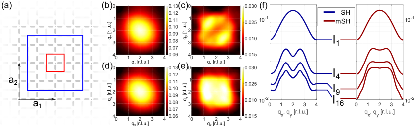
where $I(\mathbf{q})$ is the intensity for a given scattering vector $\mathbf{q}$ in reciprocal space, $N$ denotes the number of spins over which the SSF is calculated, $\mathbf{S}^{\perp}_{i}$ the spin component perpendicular to $\mathbf{q}$ and $\mathbf{r}_{i}$ is the position of the corresponding spin in the real-space lattice. The SH and the mSH lattices have different lattice points, $\mathbf{r}_{i}$ , for the long- and two short-mesospins, the differences in the SSF of the SH and mSH data is dominated by this structural difference. To facilitate a proper comparison between the two cases, only the mesospin sub-set found in both geometries, namely the four-fold coordinated vertices, has been taken into account for the SSF computation. Therefore we calculate the SSF according to equation (1), in the same manner as is explained in more detail by Östman et al.¹⁰, but only using the mesospins of the vertices with a coordination number of four. Since this sub-lattice of mesospins is the same in both the SH and mSH lattices, differences in the SSF represent different ordering among these sub-sets of spins. Characteristic SSF maps for the SH and mSH networks are presented in Fig. 4.

Although neither of the two maps presents specific features, such as pinch points or Bragg peaks, their diffuse signals systematically exhibit clear differences. This is indicative of differences in the global spin order, which have not been captured by the statistics determined on the vertex-level (presented in Fig. 3(d) and 3(e) ). The striking feature is the presence of a hollow region ( $\it{e.g.}$ at the ( $\pm$ 2, $\pm$ 2) (r.l.u.) points in reciprocal space) in the SH lattice SSF map, with the same region having a more uniform intensity distribution in the structure factor map of the mSH. To understand the origin of this effect and identify the length-scales that are at play, we have computed magnetic structure factors for networks of gradually-increasing size and network-averaged these individual signals for each chosen network-size. Since the sample is large enough to assume ergodic conditions, this size reduction of the sampling window and the corresponding network-averaging, provides statistical information about the magnetic state on the length-scale of the sampling window rather than the high spatial frequencies of the speckle pattern (Fig. 4) obtained from the specific global microstate.

Hence, we define

I_{L}=\frac{1}{\left({4L}\right)^{2}M}\sum_{m=1}^{M}\sum_{(i,j=1)}^{4L}\mathbf{S}^{\perp}_{i}\cdot\mathbf{S}^{\perp}_{j}\cdot e^{i\mathbf{q}\cdot(\mathbf{r}_{i}-\mathbf{r}_{j})}

(2)

as an incoherent²⁴ spatial average over sampling windows with $L$ four-fold coordinated vertices. Each sampling window therefore consists of $4L$ spins (taking into account only the short-mesospins). The SSF $I_{L}$ is the average of all $M$ sampling windows present in the measured global microstate.

Fig. 5(b) and 5(d) show a comparison of $I_{1}$ , i.e. the averaged SSF for a single four-fold coordinated vertex (four mesospins) for the SH and mSH lattices. Both are virtually indistinguishable, which is not surprising since $I_{1}$ is merely a different representation of the vertex statistics shown in Fig. 3(d). In other words, as the vertex statistics showed no significant differences, the SSF maps in Fig. 5(b) and Fig. 5(d) should also be similar, traceable also in a comparison of the top-most diagonal line-profiles in Fig. 5(f). Expanding the SSF input window to sixteen mesospins ( $I_{4}$ , four four-fold coordinated vertices), a clear difference between the SH and mSH appears, with a more pronounced dip in the intensity at the (2,2) reciprocal space position for the SH lattice case (Fig. 5(f) ). Expanding the real space input window to thirty-six mesospins ( $I_{9}$ , nine four-fold coordinated vertices), the differences in the SSF maps between the SH (Fig. 5(c) ) and mSH (Fig. 5(e) ) become even more pronounced (see also the line-profiles in Fig. 5(f) ). The line-profiles in Fig. 5(f) are diagonal cuts through the respective SSF maps $I_{1}$ , $I_{4}$ , $I_{9}$ and $I_{16}$ from reciprocal space position (q_x, q_y) = (0, 0) [r.l.u.] to (q_x, q_y) = (4, 4) [r.l.u.]. The results from these spatially-limited SSF maps in Fig. 5 are qualitatively similar to the features observed for the SSF of the full microstate in Fig. 4 and capture differences in the magnetic short-range order, exceeding the extension of just one vertex.

III.5 Short-range magnetic order

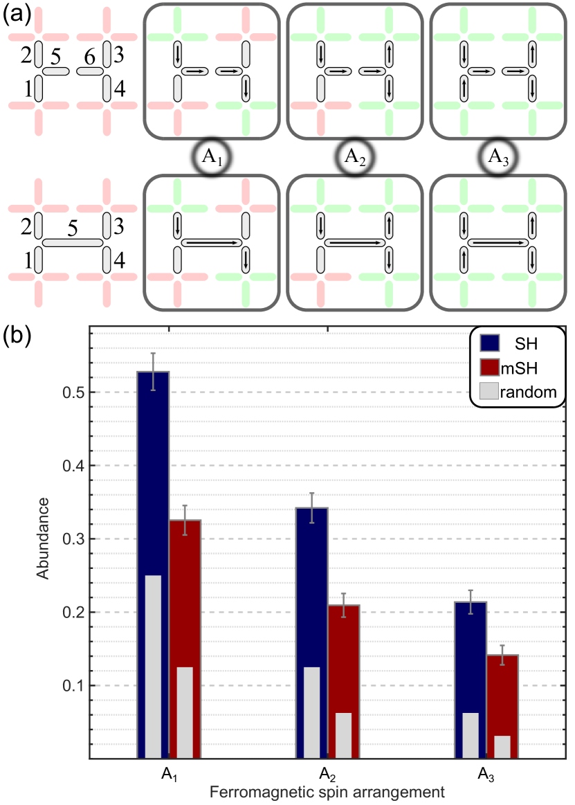
We attribute the origin of the features observed in the SSF maps to the long elements in the SH lattice and the difference in activation energies between the short and long islands. To elaborate more on this premise, we have extracted the abundance of various spin arrangements that connect four-fold coordinated vertices across a Type-I₂ vertex in the mSH lattice or a long-mesospin in the SH lattice. Here, we focus on three of the different configurations of interest for such spin arrangements, as presented in Fig. 6(a). In the three vertex coupling classes, A₁, A₂ and A₃, a total of nine different ferromagnetic spin arrangements are investigated. A detailed analysis of all nine spin arrangements can be found in the Supplementary Materials Fig. 3. In Fig 6(b) we report their abundances for both lattices, along with the estimated values given by a random distribution, in the absence of any interaction between the considered mesospins. A₁ and A₂ are averages of four different spin arrangements (C₁-C₄ and C₅-C₈, see Supplementary Materials Fig. 3), which have the same characteristic. In the case of A₁, one mesospin (mesospin 1 or 2 in schematic 6(a) ) is ferromagnetically aligned to the long-mesospin (or the two ferromagnetically aligned mesospins of the two-fold coordinated vertex) and one mesospin on the other side (mesospin 3 or 4 in Fig. 6(a) ). For A₂ one mesospin on one side is ferromagnetically aligned with two mesospins on the other side of the long-mesospin (or the two ferromagnetically aligned mesospins of the two-fold coordinated vertex). A₃ represents the lowest energy configuration for these five (six in the mSH) mesospins and arranges all mesospins (mesospin 1, 2, 3 and 4 in schematic Fig. 6(a) ) ferromagnetically with respect to the long-mesospin (or the two ferromagnetically aligned mesospins of the two-fold coordinated vertex).

IV Discussion

The spin arrangements in Fig. 6 highlight the development of a stronger correlation between four-fold coordinated vertices across a long-mesospin in the SH lattice than in the mSH, in which case the coupling is mediated via a two-fold coordinated vertex. In the Shakti ground state manifold as described by Chern et al.¹⁹, the four-fold coordinated vertices are always in their lowest energy state, Type-I₄ (see definition Fig. 3c). This state has a two-fold degeneracy, which we denote by Type-I₄(A) and Type-I₄(B) (see Supplementary Materials Fig. 4(b) ). A transition from Type-I₄(A) to a Type-I₄(B) is given by a magnetization reversal of all four mesospin. Two Type-I₄ vertices which are ferromagnetically coupled via a Type-I₂ or a long-mesospin will always be of opposite states, Type-I₄(A) and Type-I₄(B). Returning to the SSF maps in Fig. 4 and Fig. 5, the distinct shape in the SSF can be explained by the enhanced effective coupling of Type-I₄(A) to Type-I₄(B) vertices via the long-mesospins in the SH lattice. In other words, although the long-mesospins freeze in a random configuration, they are more effective in transmitting magnetic correlations from one end of a Shakti plaquette to the other, than the two-fold vertex of the mSH lattice. While this is a rather straightforward result for the case of one plaquette, it is a priori expected that, on the lattice scale, the prior establishment of a random distribution of long-mesospin states would yield an even more randomized configuration of short islands, a fact that the mSH lattice might circumvent given the absence of these constraints.

To further discuss our results we would like to compare them with the ones previously reported by Gilbert et al.²⁰. For the strong coupling regime, they observed an almost perfect ground-state ordering of the four-fold coordinated vertices for the mSH lattice, while the SH lattice has only about 80% of these vertices in the lowest energy state, Type-I₄. These differences, in the light of our results, can be attributed to the distinct energy-scales. As the long-mesospins freeze into a pre-defined disordered sub-lattice, the Shakti ground state manifold is restricted and shaped by the long-mesospin sub-lattice. When coupling four Type-I₄ vertices via a long-mesospin, 16 different Type-I₄-tilings are possible. The Shakti ground state, as defined by Chern et al.¹⁹, can be obtained with only 12 out of the total 16 tilings. The mSH lattice, with its mono-sized short-mesospins, can access the entire ensemble of tilings. However, the pre-defined disordered long-mesospin arrangement effectively reduces the possible states in the Shakti ground state manifold (see Supplementary Materials Fig. 4). The frozen long-mesospin restricts the Type-I₄-tiling amongst four four-fold coordinated vertices to 7 out of 16 possible arrangements. As the system grows in size, the Shakti ground state manifold is further reduced by each added frozen long-mesospin (for further information see Supplementary Materials). This is a plausible cause for the higher order found in the mSH lattice for the strong-coupling regime reported by Gilbert et al.²⁰ compared to the SH lattice. However, as the inter-island coupling strength is reduced, the long-mesospins, although a source of randomness, provide a better locally-correlated state than the two-fold coordinated vertices of the mSH lattice.

V Conclusions

Using thermally-active nano-patterned arrays of weakly-coupled magnetic mesospins, we have highlighted the impact of distinct length- and energy-scales on the development of magnetic order in artificial spin ice. While our study is restricted to the Shakti geometry and the weak-coupling regime, it captures the importance of the energy hierarchy in mesoscopic architectures and its role for the obtained magnetic order. Given the vast opportunities in geometrical design and the available choices of magnetic materials, the energy hierarchy can be engineered, and, in combination with suitable thermal or even demagnetization protocols, used as a tool for tailoring the magnetic order in mesoscopic magnetic structures. The hierarchy of the energy-scales, as well as the interplay between them, lie behind the complex emergent behavior and properties seen frequently across a range of natural systems²⁵. Artificial spin systems provide, therefore, a unique opportunity to study emergence, by offering a ‘designer’ fabrication route and parametrization of the relevant variables. This opportunity potentially allows for a better understanding of problems in physics requiring multiple scale-analysis²⁶.

VI Acknowledgments

The authors would like to thank C. Nisoli and G.W. Chern for valuable discussions. The authors acknowledge support from the Knut and Alice Wallenberg Foundation, the Swedish Research Council and the Swedish Foundation for International Cooperation in Research and Higher Education. The patterning was performed at the Center for Functional Nanomaterials, Brookhaven National Laboratory, supported by the U.S. Department of Energy, Office of Basic Energy Sciences, under Contract No. DE-SC0012704. This research used resources of the Advanced Light Source, which is a DOE Office of Science User Facility under contract No. DE-AC02-05CH11231. U.B.A. acknowledges funding from the Icelandic Research Fund grants Nr. 141518 and 152483.

References

(1) R. F. Wang, C. Nisoli, R. S. Freitas, J. Li, W. McConville, B. J. Cooley, M. S. Lund, N. Samarth, C. Leighton, V. H. Crespi, and P. Schiffer, Artificial spin ice in a geometrically frustrated lattice of nanoscale ferromagnetic islands, Nature 439, 303–306 (2006).
(2) C. Nisoli, R. Moessner, and P. Schiffer, Colloquium: Artificial spin ice: Designing and imaging magnetic frustration, Rev. Mod. Phys. 85, 1473–1490 (2013).
(3) I. Syôzi, Statistics of Kagomé Lattice, Progress of Theoretical Physics 6, 306–308 (1951).
(4) E. H. Lieb, Exact Solution of the $F$ Model of An Antiferroelectric, Phys. Rev. Lett. 18, 1046–1048 (1967).
(5) E. H. Lieb, Residual Entropy of Square Ice, Phys. Rev. 162, 162–172 (1967).
(6) S. Zhang, I. Gilbert, C. Nisoli, G.-W. Chern, M. J. Erickson, L. O’Brien, C. Leighton, P. E. Lammert, V. H. Crespi, and P. Schiffer, Crystallites of magnetic charges in artificial spin ice, Nature 500, 553–557 (2013).
(7) B. Canals, I.-A. Chioar, V.-D. Nguyen, M. Hehn, D. Lacour, F. Montaigne, A. Locatelli, T. O. Menteş, B. S. Burgos, and N. Rougemaille, Fragmentation of magnetism in artificial kagome dipolar spin ice, Nature Communications 7, 11446 (2016).
(8) Y. Perrin, B. Canals, and N. Rougemaille, Extensive degeneracy, Coulomb phase and magnetic monopoles in artificial square ice, Nature 540, 410–413 (2016).
(9) C. Nisoli, V. Kapaklis, and P. Schiffer, Deliberate exotic magnetism via frustration and topology, Nature Physics 13, 200–203 (2017).
(10) E. Östman, H. Stopfel, I.-A. Chioar, U. B. Arnalds, A. Stein, V. Kapaklis, and B. Hjörvarsson, Interaction modifiers in artificial spin ices, Nature Physics 14, 375–379 (2018).
(11) J. P. Morgan, A. Stein, S. Langridge, and C. H. Marrows, Thermal ground-state ordering and elementary excitations in artificial magnetic square ice, Nature Physics 7, 75–79 (2011).
(12) U. B. Arnalds, A. Farhan, R. V. Chopdekar, V. Kapaklis, A. Balan, E. T. Papaioannou, M. Ahlberg, F. Nolting, L. J. Heyderman, and B. Hjörvarsson, Thermalized ground state of artificial kagome spin ice building blocks, Applied Physics Letters 101, 112404 (2012).
(13) A. Farhan, P. M. Derlet, A. Kleibert, A. Balan, R. V. Chopdekar, M. Wyss, L. Anghinolfi, F. Nolting, and L. J. Heyderman, Exploring hyper-cubic energy landscapes in thermally active finite artificial spin-ice systems, Nature Physics 9, 375–382 (2013).
(14) A. Farhan, P. M. Derlet, A. Kleibert, A. Balan, R. V. Chopdekar, M. Wyss, J. Perron, A. Scholl, F. Nolting, and L. J. Heyderman, Direct Observation of Thermal Relaxation in Artificial Spin Ice, Physical Review Letters 111, 057204 (2013).
(15) V. Kapaklis, U. B. Arnalds, A. Harman-Clarke, E. T. Papaioannou, M. Karimipour, P. Korelis, A. Taroni, P. C. W. Holdsworth, S. T. Bramwell, and B. Hjörvarsson, Melting artificial spin ice, New Journal of Physics 14, 035009 (2012).
(16) V. Kapaklis, U. B. Arnalds, A. Farhan, R. V. Chopdekar, A. Balan, A. Scholl, L. J. Heyderman, and B. Hjörvarsson, Thermal fluctuations in artificial spin ice, Nature Nanotechnology 9, 514–519 (2014).
(17) Y. Lao, F. Caravelli, M. Sheikh, J. Sklenar, D. Gardeazabal, J. D. Watts, A. M. Albrecht, A. Scholl, K. Dahmen, C. Nisoli, and P. Schiffer, Classical topological order in the kinetics of artificial spin ice, Nature Physics (2018), in press.
(18) M. J. Morrison, T. R. Nelson, and C. Nisoli, Unhappy vertices in artificial spin ice: new degeneracies from vertex frustration, New Journal of Physics 15, 045009 (2013).
(19) G.-W. Chern, M. J. Morrison, and C. Nisoli, Degeneracy and Criticality from Emergent Frustration in Artificial Spin Ice, Physical Review Letters 111, 177201 (2013).
(20) I. Gilbert, G.-W. Chern, S. Zhang, L. O’Brien, B. Fore, C. Nisoli, and P. Schiffer, Emergent ice rule and magnetic charge screening from vertex frustration in artificial spin ice, Nature Physics 10, 670–675 (2014).
(21) M. Pärnaste, M. Marcellini, E. Holmström, N. Bock, J. Fransson, O. Eriksson, and B. Hjörvarsson, Dimensionality crossover in the induced magnetization of Pd layers, Journal of Physics: Condensed Matter 19, 246213 (2007).
(22) W. Wernsdorfer, E. Orozco, K. Hasselbach, A. Benoit, B. Barbara, N. Demoncy, A. Loiseau, H. Pascard, and D. Mailly, Experimental Evidence of the Néel-Brown Model of Magnetization Reversal, Physical Review Letters 78, 1791–1794 (1997).
(23) A. Farhan, C. F. Petersen, S. Dhuey, L. Anghinolfi, Q. H. Qin, M. Saccone, S. Velten, C. Wuth, S. Gliga, P. Mellado, M. J. Alava, A. Scholl, and S. van Dijken, Nanoscale control of competing interactions and geometrical frustration in a dipolar trident lattice, Nature Communications 8, 995 (2017).
(24) With the term incoherent, we mean that we do not account for the phase relationship between the averaged sampling windows. The correlations represented in the calculated SSF maps, are only up to lateral extensions of the respective sampling window size and are insensitive to correlations between or across multiple sampling windows.
(25) P. W. Anderson, More Is Different, Science 177, 393–396 (1972).
(26) K. G. Wilson, Problems in Physics with many Scales of Length, Scientific American 241, 158–179 (1979).

VII Author contributions

H.S. D.G. and A.S. fabricated the samples. H.S., E.Ö., U.B.A., and V.K. performed the PEEM-XMCD experiments. H.S., E.Ö., I.A.C., D.G, T.P.A.H., B.H. and V.K. analyzed the data and contributed to theory development. H.S., I.A.C., B.H. and V.K. wrote the manuscript. All authors discussed the results and commented on the manuscript.